Depth estimation from 4D light field videos

Abstract

Depth (disparity) estimation from 4D Light Field (LF) images has been a research topic for the last couple of years. Most studies have focused on depth estimation from static 4D LF images while not considering temporal information, i.e., LF videos. This paper proposes an end-to-end neural network architecture for depth estimation from 4D LF videos. This study also constructs a medium-scale synthetic 4D LF video dataset that can be used for training deep learning-based methods. Experimental results using synthetic and real-world 4D LF videos show that temporal information contributes to the improvement of depth estimation accuracy in noisy regions. Dataset and code is available at: https://mediaeng-lfv.github.io/LFV_Disparity_Estimation.

1 INTRODUCTION

Computational photography has attracted much attention because post-image processing after shooting can synthesize photos that cannot be taken with a normal camera. Light field imaging, one of the major computational photography techniques, captures the amount of light rays from several different directions. 4D light field images (LFIs), which are represented by two spatial and two angular parameters, can be captured by camera arrays, gantries consisting of a single moving camera, and specially designed plenoptic cameras [1] such as Lytro and Raytrix. The spatial-angular information recorded in 4D LFIs has been exploited to improve the performance of many computer vision applications, such as digital refocusing [1], image segmentation, material classification, super-resolution, and, most recently, depth estimation  [2, 3, 4].

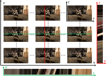
(a) 4D LFI and corresponding horizontal and vertical EPIs.

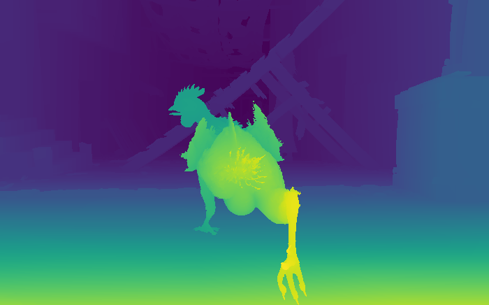
(b) The ground-truth depth (disparity) map corresponding to central view of 4D LFI.

Figure 1: Exsample of the 4D LFV dataset developed in this study.

Depth estimation from 4D LFIs has been a research topic for the last few years. Due to plenoptic cameras’ structure, the baseline between sub-aperture images is very narrow and there exists a trade-off between the spatial and the angular resolution. This makes depth estimation from 4D LFIs captured by a plenoptic camera challenging. Recently, deep learning-based methods [3, 4] using epipolar plane images (EPIs)(Fig. 1), which consist of two-dimensional angular-spatial slices, achieved high performance in the accuracy metrics of the HCI 4D Light Field Benchmark [5], which is often used as a benchmark for evaluating 4D LFIs depth estimation methods. However, previous studies have focused on depth estimation from static 4D LFIs while no studies have considered the temporal information, i.e., 4D light field videos (LFVs). The success in monocular depth estimation considering the temporal correlations and consistency among consecutive video frames  [6] suggests that the temporal information can also help 4D LF-based depth estimation.

Therefore, this paper proposes a depth estimation neural network using 4D LFV as input. The proposed method estimates depth maps of scenes by extracting the spatial-angular information from the EPIs volume at each frame and by collecting the temporal information using Convolutional Long Short-Term Memory (CLSTM).

The contributions of this study are summarized as follows:

• This study developed a medium-scale synthetic 4D LFV dataset that can be used for training deep learning-based methods from the open-source movie “Sintel” [7].

• To the best of our knowledge, this is the first study on depth estimation from the spatial-angular-temporal information recorded in a 4D LFV.

• Experimental results using synthetic and real-world 4D LFVs showed that the temporal information helps to improve 4D LF-based depth estimation performance.

In this study, the target value estimated by the proposed method is the disparity (Fig. 1). Since the disparity and depth can be transformed into each other, this paper uses these terms indistinguishably where it is not necessary to make the distinction between them to facilitate the reader’s understanding.

2 Related works

2.1 4D LFIs depth estimation methods

Over the past few years, many deep learning-based depth estimation methods from 4D LFIs have been proposed with great success [8, 9, 3, 4]. Such methods improve both accuracy and runtime compared to conventional optimization-based methods [2, 10]. Heber et al. proposed a method that predicts the slope of lines in EPI using convolutional neural network (CNN) combined with by the high-order regularization [8]. They also succeeded in producing high-quality results at low computational cost by extracting geometric information from a LFI using a U-shaped encoder-decoder architecture [9] . Shin et al. [3] proposed a fully convolutional neural network with fast and accurate performance in depth estimation. They introduced a multi-stream architecture consisting of multiple inputs of sub-aperture image stacks along four angular directions (horizontal, vertical, left- and right-diagonal). Faluvégi et al. [4] showed that, by applying 3D convolution in each stream, the performance was maintained even when only two angular directions (horizontal, vertical) were used instead of the four directions.

2.2 Monocular depth estimation methods

With the success of CNN in image recognition, many deep learning-based monocular depth estimation methods have been proposed, and some of them estimate depth values from videos by considering the temporal information  [11, 12, 6]. Karsch et al. [11] proposed a method to produce temporally consistent depth maps using local motion cues and optical flow. Zhou et al. [12] proposed a method that simultaneously estimates depth and camera pose using bundle adjustment and recovers the details of the estimated depth map using a super-resolution network. Zhang et al. [6] proposed a video depth estimation framework that captures spatial features as well as temporal correlations between consecutive video frames using CLSTM. In this framework, the trained deep CNN extracts the spatial features from video frames and the subsequent CLSTM collects temporal correlations to estimate depth values. Their framework can handle various kinds of spatial feature extraction network, and thus can be applied to other video depth estimation methods with minimum modification.

3 The proposed method

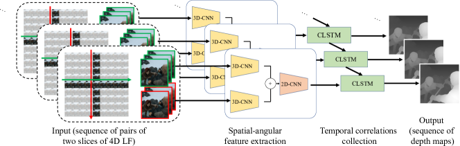
Figure 2: The proposed architecture.

This paper proposes a neural network architecture for depth estimation from 4D LFV, which builds on top of the findings of the previous studies [10, 4]. The proposed architecture uses a temporal sequence of two image stacks of horizontal and vertical slices of 4D LFV frames as input. Fig. 2 shows the proposed architecture consisting of two modules: (1) the first module for the spatial-angular feature extraction from two LF slices (horizontal and vertical) using two-stream 3D CNN, and (2) the second module for depth estimation by collecting the temporal information of the spatial-angular features using CLSTM [6].

3.1 Two-stream 3D CNN for extracting the spatial-angular features

The proposed method adopts a two-stream structure to extract meaningful representations of the horizontal and vertical directions from the sub-aperture images sliced in their direction. Focusing on Faluvegi et al. [4]’s model, which benefits from having fewer parameters to be trained, the proposed method employs 3D CNN for spatial-angular feature extraction. Here, the viewpoint (angle) index is the third spatial dimension for the 3D convolution, since the slope of lines in EPIs (Fig. 1) represents depth. In the following, we describe an example of a 4D LF with an angular resolution of $9\times 9$.

Each of the two streams that process the horizontal and vertical sub-aperture image stacks first applies preprocesses consisting of two steps. First, zero-mean normalization is applied to the input data in batches, resulting in better emphasizing the differences in the lines of EPIs and making it easier for the network to learn. Next, a spatial padding of $4\times 4$ is applied so that the spatial dimension of the feature maps can be maintained when applying 3D convolution.

Each stream consists of four consecutive 3D convolutional layers with kernel size $3\times 3\times 3$ and stride size one. The number of feature maps to be output is 32 in the first convolutional layer and 64 in the remaining three layers. The four 3D convolutional layers reduce the dimension of feature maps corresponding to the number of views from nine to one while keeping the spatial dimension the same size as the input.

The two feature map sets obtained from the two streams are concatenated (totally 128 maps) and input into the next five 2D convolutional layers in order to produce higher level representation. The proposed method uses 2D convolutional layers with kernel size $3\times 3$ and zero padding to maintain the feature map size. The number of feature maps gradually decreases to 64, 32, 32, 32, and 16 as passing through the five convolutional layers.

All of the above 2D and 3D convolutional layers use rectified linear unit as the activation function, and all kernel weights are initialized with Glorot initialization.

3.2 CLSTM for collecting the temporal information

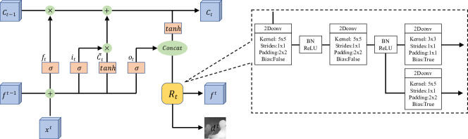
Figure 3: CLSTM structure of the proposed method.

As the input frames are continuous in the temporal dimension, taking the temporal information of these frames into consideration may help to estimate the depth. Following the previous work [6], the proposed method employs CLSTM shown in Fig. 3 for collecting the temporal information of the spatial-angular features extracted by CNN (Sec. 3.1). In this study, the number of feature maps in the hidden state $f^{t}$ is set to eight.

3.3 Loss function

This study employs the loss function proposed by Hu et al. [13] to train the network. While Hu et al. adopted the logarithm of the difference between the estimated and ground-truth depth value, this study uses the difference directly as a loss since the proposed method estimates disparity that is inversely proportional to depth. The loss function $L$ consists of three terms, designed to penalize inaccurate disparity estimations, the errors around edges, and small structural errors such as high-frequency undulation of a surface, respectively:

$$L =l_{disparity}+\lambda l_{grad}+\mu l_{normal}$$ (1)

$$l_{disparity} =\frac{1}{n}\sum^{n}_{i=1}\|d_{i}-g_{i}\|_{1}$$

$$l_{grad} =\frac{1}{n}\sum^{n}_{i=1}\left(\|\nabla_{x}(d_{i})-\nabla_{x}(g_{i})\|_{1}+\|\nabla_{y}(d_{i})-\nabla_{y}(g_{i})\|_{1}\right)$$

$$l_{normal} =\frac{1}{n}\sum^{n}_{i=1}\left(1-\frac{\eta^{d}_{i}\cdot\eta^{g}_{i}}{\sqrt{\eta^{d}_{i}\cdot\eta^{d}_{i}}\sqrt{\eta^{g}_{i}\cdot\eta^{g}_{i}}}\right)\,,$$

where $\lambda$ and $\mu$ are weighting coefficients. $n$ denotes the number of pixels; $d_{i}$ and $g_{i}$ are the estimated and ground-truth disparity of pixel $i$, respectively. $\nabla_{x}$ and $\nabla_{y}$ represent the spatial derivative along the $x$-axis and $y$-axis respectively. $\eta^{d}_{i}=[-\nabla_{x}(d_{i}),-\nabla_{y}(d_{i}),1]$ and $\cdot$ denotes inner product.

4 4D Light field video dataset

This study developed the Sintel 4D LFV dataset from the open-source movie “Sintel” [7] (Fig. 1) because it was difficult to accurately evaluate the effectiveness of deep learning-based 4D LFVs depth estimation methods with existing 4D LFV datasets [14, 15] due to small number of samples or the lack of ground-truth disparity values.

The generated dataset consists of 23 synthetic 4D LFVs with $1,204\times 436$ pixels, $9\times 9$ views, and 20–50 frames, and includes the ground-truth disparity values in the central view, so that it can be used for training deep learning-based methods.

Each scene was rendered with a “clean” pass after modifying the production file of “Sintel” with reference to the MPI Sintel dataset [16]. A “clean” pass includes complex illumination and reflectance properties including specular reflections, such as smooth shading and specular reflections, while bokeh, motion blur, and semi-transparent objects are excluded. The 4D LFVs were captured by moving the camera with a baseline of 0.01[m] towards a common focus plane while keeping the optical axes parallel. The ground-truth disparity value was obtained by transforming the depth value obtained in Blender.

5 Experiments

The performance of the proposed method is evaluated using the Sintel 4D LFV dataset and the real-world 4D LFVs [14]. By comparing with the conventional method [4] as the baseline that does not consider the temporal information, we examined whether the temporal information contributes to improve the depth estimation performance. The baseline method has a structure that replaces the CLSTM module of the proposed method with a 2D convolutional layer producing a single feature map.

5.1 Experimental setup

In the experiments, 23 scenes in the Sintel 4D LFV dataset created in Sec. 4 were divided into three subsets, i.e., 16 scenes that were used for training, three scenes for validation and four scenes for test. In total, we extracted about 1.4M patch samples with a spatial resolution of $32\times 32$ and a frame length of five using a spatial stride of 16 and a temporal stride of one. By the scene-wise splitting, about 1M, 130K and 300K samples were allocated to the training, validation and test data, respectively.

Parameters were configured as follows: The upper limit of epoch and the batch size were set to 20 and 64, respectively. Adam optimizer [17] was employed. The learning rate started at 0.0005 and was decreased by a factor of 0.1 after 10 and 15 epochs. The weights $\lambda$ and $\mu$ of loss function $L$ were set as $\lambda=1$ and $\mu=1$. It took about four days for the proposed network to be trained on a computer with a NVIDIA GTX 1080Ti.

The results were measured using mean square error (MSE) and bad pixel ratio (BadPix), which are common in 4D LFIs depth estimation [5]. The definition of BadPix is the percentage of pixels whose absolute errors exceed the specified threshold, i.e., $\|d_{i}-g_{i}\|_{1}>t$, where $t$ is the threshold. Three thresholds are often used for calculating the bad pixel ratios: 0.01, 0.03, and 0.07. These values were calculated based on $1,024\times 432$ depth maps that were reconstructed by combining the depth estimation results for test patches.

5.2 Results

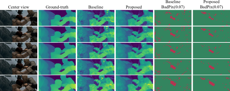
Figure 4: The estimation results of the proposed method and the baseline method [4].

Table 1: Comparisons of the propsed method and the baseline method [4] on the test scenes of the Sintel 4D LFV dataset.

ambushfight5
Method	MSE*100	BadPix(0.07)	BadPix(0.03)	BadPix(0.01)
Baseline [4]	0.2590	11.005	30.3701	65.4103
Proposed	0.2167	8.3404	22.8762	62.0493
bamboo3
Method	MSE*100	BadPix(0.07)	BadPix(0.03)	BadPix(0.01)
Baseline [4]	0.2895	12.1862	29.2804	57.9944
Proposed	0.2159	8.9475	21.8162	53.2985
shaman2
Method	MSE*100	BadPix(0.07)	BadPix(0.03)	BadPix(0.01)
Baseline [4]	3.391	37.9157	53.4889	75.6842
Proposed	2.4421	32.7585	50.6706	74.7733
thebigfight2
Method	MSE*100	BadPix(0.07)	BadPix(0.03)	BadPix(0.01)
Baseline [4]	0.0305	1.0964	4.4142	18.6974
Proposed	0.0367	1.0688	3.6084	17.7493

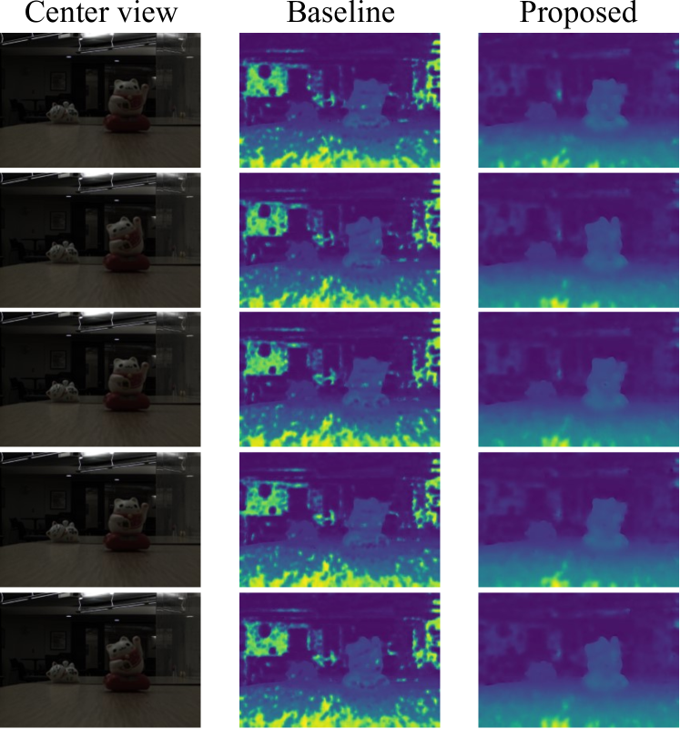
Figure 5: The results of real-world data.

Table 5 shows the performance of the proposed method and the baseline method [4] that does not consider the temporal information on the four test scenes. In most of the test scenes, the proposed method achieved better performance than the baseline by considering the temporal information. Focusing on the results of thebigfight2, the proposed method was slightly inferior in MSE but superior in BadPix, indicating that the proposed method estimated better disparity values in regions that were difficult to estimate for the baseline method.

Fig. 5 shows example estimation results for ambushfight5 scene, which included noisy textured rock surfaces and two characters fighting. As can be seen from Fig. 5, by using the temporal information the proposed method can estimate a better disparity map with a smoother surface in noisy regions than the baseline method.

On the other hand, some regions were difficult to estimate the depth even for the proposed method, e.g. the occipital region in the image center. This region corresponded to textureless regions defined by Shin et al. [3], i.e., the mean absolute difference between a center pixel and other pixels in the patch was less than 0.02.

In addition to the synthetic data, this study also tested the proposed method using real-world 4D LFVs [14]. The real-world data captured by a light field camera is challenging as they contain severe image noise due to the inherent structural problem in the camera. Fig. 5 shows the disparity estimation results using the model trained on the Sintel 4D LFV dataset. We observed that the proposed method provided more natural disparity estimation than the baseline method. The results also showed that the synthetic 4D LFV dataset created in this study was sufficiently realistic to train deep neural networks.

6 Conclusions

This paper proposes an end-to-end neural network architecture for depth estimation from 4D LFV. The proposed method employs two-stream CNN and CLSTM to process the spatial-angular-temporal information recorded in a 4D LFV. This study also constructs a synthetic 4D LFV dataset from the open-source movie “Sintel” [7], which can be used for training deep learning-based methods. Experimental results showed that the temporal information contributed to the performance of 4D LF-based depth estimation and that depth estimation was possible even in noisy real-world data.

References

- [1] Ng, R., Levoy, M., Brédif, M., Duval, G., Horowitz, M., and Hanrahan, P., Light field photography with a hand-held plenoptic camera, PhD thesis, Stanford University (2005).
- [2] Tao, M. W., Hadap, S., Malik, J., and Ramamoorthi, R., “Depth from combining defocus and correspondence using light-field cameras,” ICCV , 673–680 (2013).
- [3] Shin, C., Jeon, H.-G., Yoon, Y., So Kweon, I., and Joo Kim, S., “Epinet: A fully-convolutional neural network using epipolar geometry for depth from light field images,” CVPR , 4748–4757 (2018).
- [4] Faluvégi, Á., Bolseé, Q., Nedevschi, S., Dădârlat, V.-T., and Munteanu, A., “A 3d convolutional neural network for light field depth estimation,” IC3D , 1–5, IEEE (2019).
- [5] Honauer, K., Johannsen, O., Kondermann, D., and Goldluecke, B., “A dataset and evaluation methodology for depth estimation on 4d light fields,” ACCV , 19–34, Springer (2016).
- [6] Zhang, H., Shen, C., Li, Y., Cao, Y., Liu, Y., and Yan, Y., “Exploiting temporal consistency for real-time video depth estimation,” ICCV , 1725–1734 (2019).
- [7] Roosendaal, T. (Producer), “Sintel. Durian Open Movie Project,” https://durian.blender.org/ (2010).
- [8] Heber, S. and Pock, T., “Convolutional networks for shape from light field,” CVPR , 3746–3754 (2016).
- [9] Heber, S., Yu, W., and Pock, T., “Neural epi-volume networks for shape from light field,” ICCV , 2252–2260 (2017).
- [10] Zhang, S., Sheng, H., Li, C., Zhang, J., and Xiong, Z., “Robust depth estimation for light field via spinning parallelogram operator,” CVIU 145, 148–159 (2016).
- [11] Karsch, K., Liu, C., and Kang, S. B., “Depth transfer: Depth extraction from video using non-parametric sampling,” TPAMI 36(11), 2144–2158 (2014).
- [12] Zhou, L., Ye, J., Abello, M., Wang, S., and Kaess, M., “Unsupervised learning of monocular depth estimation with bundle adjustment, super-resolution and clip loss,” arXiv:1812.03368 (2018).
- [13] Hu, J., Ozay, M., Zhang, Y., and Okatani, T., “Revisiting single image depth estimation: Toward higher resolution maps with accurate object boundaries,” WACV , 1043–1051, IEEE (2019).
- [14] Wang, T.-C., Zhu, J.-Y., Kalantari, N. K., Efros, A. A., and Ramamoorthi, R., “Light field video capture using a learning-based hybrid imaging system,” TOG 36(4), 1–13 (2017).
- [15] Brizzi, M., Battisti, F., and Neri, A., “A feature-based approach for light field video enhancement,” ICME , 1204–1209, IEEE (2019).
- [16] Butler, D. J., Wulff, J., Stanley, G. B., and Black, M. J., “A naturalistic open source movie for optical flow evaluation,” ECCV , 611–625, Springer (2012).
- [17] Kingma, D. P. and Ba, J., “Adam: A method for stochastic optimization,” arXiv:1412.6980 (2014).