DMRG study of FQHE systems in the open cylinder geometry

Abstract

The study of the fractional quantum Hall liquid state of two-dimensional electrons requires a non-perturbative treatment of interactions. It is possible to perform exact diagonalizations of the Hamiltonian provided one considers only a small number of electrons in an appropriate geometry. Many insights have been obtained in the past from considering electrons moving on a sphere or on a torus. In the Landau gauge it is also natural to impose periodic boundary conditions in only one direction, the cylinder geometry. The interacting problem now looks formally like a one-dimensional problem that can be attacked by the standard DMRG algorithm. We have studied the efficiency of this algorithm to study the ground state properties of the electron liquid at lowest Landau level filling factor $\nu=1/3$ when the interactions are truncated to the two most important repulsive hard-core components. Use of finite-size DMRG allows us to conclude that the ground state is a compressible two-electron bubble phase in agreement with previous Hartree-Fock calculations. We discuss the treatment of Coulomb interactions in the cylinder geometry. To regularize the long-distance behavior of the Coulomb potential, we compare two methods : using a Yukawa potential or forbidding arbitrary long distances by defining the interelectron distance as the chord distance through the cylinder. This allows us to observe the Wigner crystal state for small filling factor.

1 Introduction

When two-dimensional electrons are submitted to a magnetic field perpendicular to the plane of allowed motion their one-body wavefunctions are the so-called Landau orbitals that form a regularly spaced ladder of states, the Landau levels, and each member of the ladder has the same degeneracy given by the ratio of the magnetic flux through the sample and the elementary flux quantum $N_{\Phi}=\Phi/\Phi_{0}$. When the electron density is such that an integer number of these levels is filled, we are in the conditions of the integer quantum Hall effect and the physics of this situation can be understood essentially without considering interactions. However when there is partial filling the electrons form a remarkable state of matter, incompressible liquids with excitations possessing fractional charge as well as fractional statistics. This is the fractional quantum Hall effect (FQHE). These liquids appear for special rational values of the filling factor $\nu=N_{e}/N_{\Phi}$. The most prominent state appears in the lowest Landau level for $\nu=1/3$. From a theoretical point of view we are facing a tough problem because the kinetic energy is frozen in a Landau level and the fate of electrons is decided entirely by the two-body Coulomb interactions. So no perturbative approach is feasible. One tool that has proven very fruitful is exact diagonalization (ED) of systems of few electrons when the Fock space is small enough to store a handful of vectors in computer memory allowing use of Krylov subspace methods. However the limitations on the number of electrons is too severe to consider problems involving for example additional degeneracies like spin or valley degrees of freedom that are very important in the physics of two-dimensional materials like graphene. It has long been noted that since the Landau gauge orbitals can be naturally indexed by an integer, the projected Coulomb interaction is formally a one-dimensional problem albeit with long-range interactions. It is thus possible to use the density matrix renormalization group algorithm [1, 2, 3] to FQHE provided one chooses the correct geometry. Recent progresses have been done in this direction [4, 5, 6, 7, 8, 9, 10, 11, 12, 13, 14]. here we present the use of DMRG in the geometry of a cylinder with open boundaries which has been explored already by ED. We made use of the modern C++ library ITensor (version 3.1) [3]. The DMRG gives easy access to an approximation of the ground state wavefunction from which one can compute observables. We take profit of this feature to obtain the pair correlation function, a standard diagnostic tools for the properties of quantum liquids.

The section (2) defines what we call the cylinder geometry with open boundary conditions. In section (3) we present a study of a special truncated interaction between electrons. We investigate the case of the Coulomb interaction in section (4). Finally section (5) contains our conclusions.

2 The open cylinder geometry for FQHE

In the Landau gauge the one-body eigenstates spanning the lowest Landau level are given by :

$$\phi_{n}(x,y)=\left(\frac{1}{Ll\sqrt{\pi}}\right)^{\frac{1}{2}}\exp\left(-\frac{1}{2l^{2}}(x-x_{n})^{2}\right)\exp\left(ik_{n}y\right),$$ (1)

where :

$$k_{n}=\frac{2\pi n}{L},\quad x_{n}/l=-\frac{2\pi nl}{L}.$$ (2)

Here we have imposed periodic boundary conditions along the $y$ direction $\phi(y)=\phi(y+L)$, leading to quantization of momentum $k_{n}$. The integer $n$ can be positive or negative and defines also the center of the Gaussian wavepacket in the $x$ direction. We have used $l=\sqrt{\hbar/eB}$ which is the magnetic length, set to unity in the rest of the paper. In the following we consider finite cylinders, obtained by considering a finite number $N_{\rm orb}$ of orbitals. So we truncate the Hilbert space, constraining the integer $n$ to take only $N_{\rm orb}$ different values. It is important to note that while such a truncation is mathematically convenient it is not produced by imposing some physical hard-wall condition since the one-body eigenstates have a Gaussian shape in $x$ so formally extend far away (but with fast decay). The model does therefore not have a sharp boundary in real space. Since the spacing in the $x$ direction between two consecutive orbitals is $\delta x=2\pi/L$, the length in $x$ of the cylinder is of order $L_{x}\simeq N_{\rm orb}\delta x=2\pi N_{\rm orb}/L$. For an odd number $N_{\rm orb}$ of orbitals we restrict the index $n$ to be in $-(N_{\rm orb}-1)/2\leq n\leq(N_{\rm orb}-1)/2$, and for even $N_{\rm orb}$ we take $-N_{\rm orb}/2+1\leq n\leq N_{\rm orb}/2$. In the following we will denote by $\mathcal{I}$ this set of integers. So we see that there are two independent parameters ruling the spatial extent in this geometry : the perimeter $L$ of the cylinder and the $x$ extent of the region where electrons can roam. Fixing the electron number $N_{e}$ and the filling factor means that we fix the number of orbitals and thus $x$ extent, the only remaining parameter is then the length $L$. It is intuitively obvious that this length should be scaled with $N_{e}$ as the numbers of particles and orbitals grow, so that the region allowed to electron motion is more or less square [15, 16, 17]. Strong deviations from this case leads to behavior unrelated to the thermodynamic limit of a two-dimensional system. For example when $L\rightarrow 0$, the “thin torus” limit, one is led to an electrostatic problem. In the opposite “hoop” limit, $L\rightarrow\infty$, one collapses the system into a one-dimensional Luttinger liquid with no remnant of the bulk.

The second-quantized formula of a generic two-body Hamiltonian is given by :

$$\mathcal{H}=\frac{1}{2}\sum_{n_{1}n_{2}n_{3}n_{4}}\mathcal{A}_{n_{1}n_{2}n_{3}n_{4}}c_{n_{1}}^{\dagger}c_{n_{2}}^{\dagger}c_{n_{3}}c_{n_{4}}$$ (3)

where the matrix elements are related to the real space potential $V$ through

$$\mathcal{A}_{n_{1}n_{2}n_{3}n_{4}}=\int d{\bf r}_{1}d{\bf r}_{2}\,\,\phi_{n_{1}}({\bf r}_{1})^{*}\phi_{n_{2}}({\bf r}_{2})^{*}V({\bf r}_{1}-{\bf r}_{2})\phi_{n_{3}}({\bf r}_{2})\phi_{n_{4}}({\bf r}_{1}).$$ (4)

To evaluate these matrix elements it is convenient to go to momentum space :

$$\mathcal{A}_{n_{1}n_{2}n_{3}n_{4}} = \int\frac{d{\bf Q}}{(2\pi)^{2}}F_{n_{1},n_{4}}({\bf Q})F_{n_{2},n_{3}}(-{\bf Q})\tilde{V}({\bf Q}),$$ (5)

where we have defined :

$$F_{n,m}({\bf Q})=\int d{\bf r}\,\,\phi_{n}({\bf r})^{*}\phi_{m}({\bf r})e^{-i{\bf Q}\cdot{\bf r}}$$ (6)

and the Fourier transform :

$$\tilde{V}({\bf Q})=\int d{\bf R}\,\,V({\bf R})e^{i{\bf Q}\cdot{\bf R}}.$$ (7)

Due to the periodicity of the wavefunction and of the interaction in the $y$ direction we only need to consider wave-vectors ${\bf Q}$ of the form ${\bf Q}=(q_{x},q_{y}=2\pi q/L)$ with $q\in\mathbb{Z}$. In such cases the function $F$ is equal to :

$$F_{n,m}({\bf Q}=(q_{x},q_{y}=2\pi q/L))=\delta_{q,m-n}\exp\left(-\frac{1}{4}q_{x}^{2}+\frac{i}{2}q_{x}\left(k_{n}+k_{m}\right)-\frac{1}{4}\left(k_{n}-k_{m}\right)^{2}\right)$$ (8)

with $k_{i}={2\pi n_{i}}/{L}$.

In the following we will consider two versions of the $1/r$ Coulomb interaction which are adapted to the cylindrical geometry. Our use of $1/r$ means that energies are measured in units of $e^{2}/\epsilon l$ with $e$ the electric charge and $\epsilon$ the dielectric constant of the host material.

2.1 Yukawa

One standard way to make the Coulomb interaction periodic in the $y$ direction of the cylinder ($V(x,y)=V(x,y+L)$) is to use a sum over periodic images :

$$V({\bf R})=\sum_{n=-\infty}^{\infty}\frac{1}{\left|{\bf R}+Ln{\bf e}_{y}\right|}.$$ (9)

In Fourier space this is equivalent to :

$$\tilde{V}({\bf Q}=(q_{x},q_{y}))=\frac{2\pi}{\left|{\bf Q}\right|}\sum_{n=-\infty}^{\infty}e^{inLq_{y}}.$$ (10)

The above sum of exponentials is proportional to a Dirac “comb” (Poisson formula) and we obtain :

$$\tilde{V}({\bf Q})=\frac{(2\pi)^{2}}{L\left|{\bf Q}\right|}\sum_{n=-\infty}^{\infty}\delta\left(q_{y}-\frac{2\pi n}{L}\right).$$ (11)

One possibility to regularize the long-distance tail of the Coulomb interaction is by introducing some (small) Yukawa mass $\mu$. The main effect is to replace the Coulomb interaction by an exponential decay beyond the length scale $\mu^{-1}$. In that case the Fourier transform of the potential becomes :

$$\tilde{V}({\bf Q})=\frac{(2\pi)^{2}}{L\sqrt{q_{x}^{2}+q_{y}^{2}+\mu^{2}}}\sum_{n=-\infty}^{\infty}\delta\left(q_{y}-\frac{2\pi n}{L}\right).$$ (12)

This leads to an expression for the matrix elements :

$$\mathcal{A}_{n_{1}n_{2}n_{3}n_{4}}=\int_{-\infty}^{\infty}\frac{dq_{x}}{L}\sum_{n}\frac{1}{\sqrt{q_{x}^{2}+\left(\frac{2\pi n}{L}\right)^{2}+\mu^{2}}}F_{n_{1},n_{4}}(q_{x},\frac{2\pi n}{L})F_{n_{2},n_{3}}(-q_{x},-\frac{2\pi n}{L}).$$ (13)

Taking into account translation invariance we have $k_{1}-k_{3}=k_{4}-k_{2}$ and we finally obtain :

$$\mathcal{A}_{n_{1}n_{2}n_{3}n_{4}}=\frac{2\delta_{n_{1}+n_{2},n_{3}+n_{4}}}{L}\exp\left(-\frac{1}{2}\left(k_{1}-k_{4}\right)^{2}\right)\int_{0}^{\infty}\frac{dq_{x}\cos\left(q_{x}\left(k_{1}-k_{3}\right)\right)}{\sqrt{q_{x}^{2}+\left(k_{1}-k_{4}\right)^{2}+\mu^{2}}}\times\exp\left(-\frac{1}{2}q_{x}^{2}\right).$$ (14)

To obtain the matrix elements in the simulations the above integrals have to be computed numerically. Note also that for $n_{1}=n_{4}$ (and thus $n_{2}=n_{3}$) the integral is infra-red divergent when $\mu\to 0$ and we have $\mathcal{A}_{n,m,m,n}\sim|\log(\mu)|$.

2.2 Coulomb-chord potential

The disadvantage of the Yukawa potential is the presence of an extra parameter and the need to extrapolate the physical observables to $\mu\to 0$, in addition to taking thermodynamic limit ($N_{\rm orb},N_{e}\to\infty$). We now turn to another formulation of the Coulomb interaction on a cylinder. To make $V({\bf R})$ periodic in the $y$ direction of the cylinder, the Euclidean distance $d^{2}=R_{x}^{2}+R_{y}^{2}$ is replaced by the chord distance :

$$d^{2}=R_{x}^{2}+\left(\frac{L}{\pi}\right)^{2}\sin^{2}\left(\frac{\pi R_{y}}{L}\right).$$ (15)

We will now proceed to the calculation of the associated matrix elements $\mathcal{A}_{n_{1},\cdots,n_{4}}$. To do so it is convenient to use an integral representation of $1/d$ :

$$V({\bf R})=1/d=\int_{-\infty}^{\infty}\frac{d\alpha}{\sqrt{\pi}}\exp{\left(-\alpha^{2}d^{2}\right)}.$$ (16)

In Fourier space we have :

$$\tilde{V}({\bf Q})=\int d{\bf R}\int_{-\infty}^{\infty}\frac{d\alpha}{\sqrt{\pi}}\exp\left(-iq_{x}R_{x}-iq_{y}R_{y}-\alpha^{2}\left[R_{x}^{2}+\left\{\frac{L}{\pi}\sin\left(\frac{\pi R_{y}}{L}\right)\right\}^{2}\right]\right).$$ (17)

After a few simplifications (including a Gaussian integration over $R_{x}$ and then over $q_{x}$) this can be finally re-expressed as :

$$\mathcal{A}_{n_{1}n_{2}n_{3}n_{4}}=\frac{4}{\pi^{3/2}}e^{-\frac{1}{2}(k_{1}-k_{4})^{2}}\int_{0}^{\pi/2}dv\int_{0}^{\infty}\frac{d\alpha}{\sqrt{2\alpha^{2}+1}}\cos\left(vN\right)e^{-\frac{\alpha^{2}(k_{1}-k_{3})^{2}}{2\alpha^{2}+1}-\left\{\frac{\alpha L}{\pi}\sin(v)\right\}^{2}}.$$ (18)

with $N=n_{4}-n_{1}+n_{2}-n_{3}$ an even integer.

2.3 Neutralizing background

In the absence of a neutralizing background, and due to the long-range nature of the Coulomb interaction, the particles will have a strong tendency to accumulate at the edges of the cylinder. This effect is compensated by a neutralizing background. We consider the following electric charge density (of a sign opposite to that of the electrons):

$$\rho_{\rm backg.}({\bf r})=-\nu\sum_{n\in\mathcal{I}}|\phi_{n}({\bf r})|^{2}$$ (19)

where $\nu=N_{e}/N_{\rm orb}$. This charge density is not strictly uniform, but it becomes uniform in the limit of large cylinder circumference $L$. The background term in the Hamiltonian is then :

$$\mathcal{H}_{B}=\int d{\bf r}d{\bf r^{\prime}}\rho_{\rm backg.}({\bf r})V({\bf r}-{\bf r}^{\prime})\hat{\psi}^{\dagger}({\bf r^{\prime}})\hat{\psi}({\bf r^{\prime}})$$ (20)

with $\hat{\psi}({\bf r^{\prime}})=\sum_{n}\phi_{n}({\bf r^{\prime}})c_{n}$. It is also equal to :

$$\mathcal{H}_{B}=-\nu\sum_{n,m\in\mathcal{I}}A_{n,m,m,n}c^{\dagger}_{n}c_{n}=\sum_{n}B_{n}c^{\dagger}_{n}c_{n}\;\;{\rm with}\;\;B_{n}=-\nu\sum_{m}A_{n,m,m,n}.$$ (21)

There is also the electrostatic interaction energy of the background with itself :

$$\mathcal{E}_{BB}=\frac{1}{2}\int d{\bf r}d{\bf r^{\prime}}\rho_{\rm backg.}({\bf r})V({\bf r}-{\bf r}^{\prime})\rho_{\rm backg.}({\bf r^{\prime}})=\frac{\nu^{2}}{2}\sum_{n,m\in\mathcal{I}}A_{n,m,m,n}.$$ (22)

Since we work at fixed number of fermions, $\sum_{n}c^{\dagger}_{n}c_{n}=N_{e}$, the above constant can be absorbed into a uniform shift of the background potential $B_{n}\to B_{n}+\mathcal{E}_{BB}/N_{e}$.

2.4 Measurements

Simple observable quantities include the local density :

$$\rho({\bf r})=\sum_{n\in\mathcal{I}}|\phi_{n}({\bf r})|^{2}\langle c^{\dagger}_{n}c_{n}\rangle=\frac{1}{Ll\sqrt{\pi}}\sum_{n\in\mathcal{I}}\exp\left(\frac{(x-x_{n})^{2}}{l^{2}}\right)\langle c^{\dagger}_{n}c_{n}\rangle.$$ (23)

Another quantity of interest is the pair correlation function :

$$G({\bf r}_{1},{\bf r}_{2})=\sum_{i\neq j}\langle\delta({\bf r}_{1}-\hat{\bf r}_{i})\delta({\bf r}_{2}-\hat{\bf r}_{j})\rangle,$$ (24)

which can be expressed in second quantization as :

$$G({\bf r}_{1},{\bf r}_{2})=\langle\hat{\psi}^{\dagger}({\bf r}_{1})\hat{\psi}^{\dagger}({\bf r}_{2})\hat{\psi}({\bf r}_{2})\hat{\psi}({\bf r}_{2})\rangle=\sum_{i,j,k,l\in\mathcal{I}}\phi^{*}_{i}({\bf r}_{1})\phi^{*}_{j}({\bf r}_{2})\phi_{k}({\bf r}_{2})\psi_{l}({\bf r}_{1})\langle c^{\dagger}_{i}c^{\dagger}_{j}c_{k}c_{l}\rangle.$$ (25)

3 The hard-core model for spinless fermions at filling $\nu=1/3$

When projected onto the lowest Landau level, any two-body interaction can be parametrized by a discrete set of energies called the Haldane pseudopotentials. They are the exact energies of the two-body problem which is solvable in this special case. We call them $V_{m}$ and they are indexed by the relative angular momentum $m$ of the two-particle problem which is a positive integer. For spinless fermions, due to the Pauli principle only odd values matter. So a generic two-body Hamiltonian can be written as :

$$\mathcal{H}=\frac{(2\pi)^{5/2}}{L^{3}}\sum_{k}V_{k}\sum_{\{n_{i}\}}\lambda^{(n_{1}-n_{4})^{2}+(n_{1}-n_{4})^{2}}\,\,H_{k}((n_{1}-n_{2})/R)H_{k}((n_{4}-n_{3})/R)\,\,c_{n_{1}}^{\dagger}c_{n_{2}}^{\dagger}c_{n_{3}}c_{n_{4}}$$ (26)

where the first sum is over odd integers $k$ and $H_{k}$ are Hermite orthogonal polynomials. We have introduced $\lambda=\exp(-2\pi^{2}/L^{2})$ as well as the radius of the cylinder $L=2\pi R$. The thermodynamic limit requires that we go to large $L$ hence $\lambda$ should be close to unity. If we drop all $V_{k}$ except $V_{1}$ one obtains a model whose ground state for filling factor $\nu=1/3$ is exactly given by the Laughlin wavefunction. The realistic Coulomb potential has all nonzero pseudopotentials that are decreasing with increasing $k$.

Having the Laughlin wavefunction as the unique ground state of the pure $V_{1}$ Hamiltonian requires a special tuning of the number of orbitals versus the number of particles : $N_{\rm orb}=3(N_{e}-1)+1$. The constant term in this relation, dubbed “shift”, has a topological significance. It has been proposed [18] that if we consider the model Hamiltonian with now only $V_{3}$ pseudopotential then another incompressible state is obtained for $N_{\rm orb}=3N_{e}-6$. This relation leads to the same filling factor $\nu=1/3$ as the Laughlin state but with a different shift. This proposal was based on limited evidence from ED studies in the spherical geometry. Such a state if confirmed would be a new class of topological order different from the well-studied Laughlin state. We have undertaken a DMRG study of the generalized model including both $V_{1}$ and $V_{3}$ pseudopotentials to search for some change of the physical properties when interpolating between these two special Hamiltonians [22]. A simple probe of quantum liquids is the pair correlation function $g({\bf r})$. We compute it for systems of up to 30 fermions and cylinder length up to $L=22$. Sample calculations are given in Fig. (1). The top panel (a) shows $g({\bf r})$ for the pure $V_{1}$ model where we know that the physics of the Laughlin state is the correct one. The probe electron has been set at the origin of coordinates ($g({\bf r})=G({\bf r},{\bf 0})$) and there is a visible strong correlation hole around it. Beyond a ring of overdensity there is only a featureless fluid. Since we use a truncation of the number of orbitals there is a range of $x$ coordinates beyond which the density goes to zero : these are the dark boundaries in all panels. If we now increase $V_{3}$ we observe the appearance of density modulations that are like one-dimensional stripes in panel (b) and (c). Finally when tuning to the pure $V_{3}$ model in panel (d) we observe a two-dimensional pattern of density modulation. If we count the number of peaks we find that each overdensity contains exactly two electrons. This is what we expect from a bubble phase as predicted for filling factors around $\nu=1/3$ by Hartree-Fock calculations [19, 20, 21]. It has long been observed that weakening the hard-core component $V_{1}$ destroys incompressibility in the case of the Coulomb potential. Our results on a truncated model suggests that the topological order of fractional quantum Hall liquids is replaced by the simpler correlations of Hartee-Fock theory such as the bubble phase by weakening $V_{1}$. We note that extensive ED [22] in various geometries are in agreement with the compressibility of the pure $V_{3}$ model.

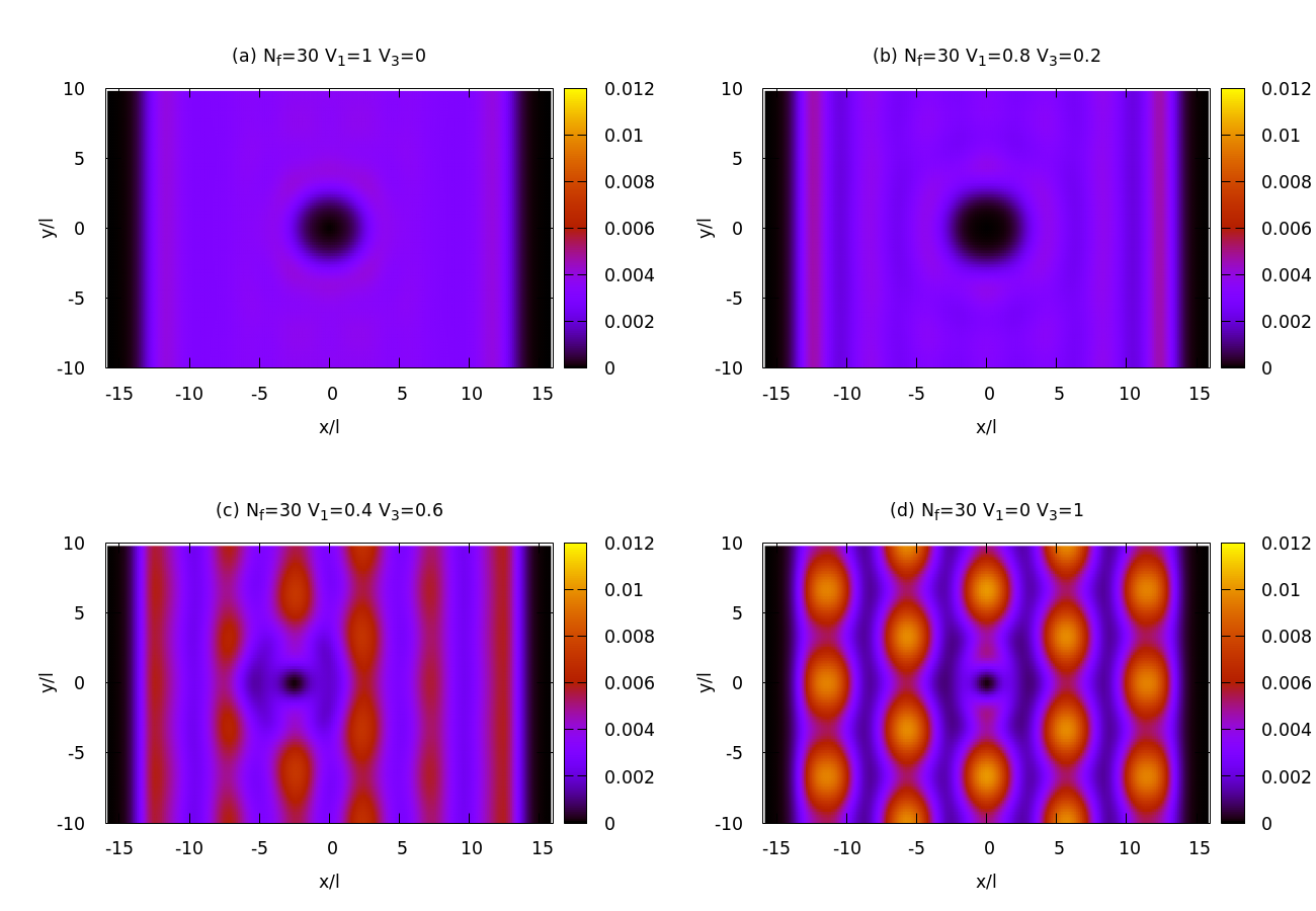
Figure 1: The pair correlation function $g(r)$ computed in real space for various models interpolating between pure $V_{1}$ and pure $V_{3}$ models. While the pure $V_{1}$ case is a featureless liquid, density modulations develop with increasing $V_{3}$. In panel (d) we observe formation of a two-dimensional structure : a triangular crystal of overdensities containing exactly two electrons per site. In panel (c) the reference electron has been offset from the center for clarity. In all cases the largest bond dimension of the matrix-product state is of the order of 8000 and the largest discarded weight varies between $\sim 6.10^{-6}$ (for $V_{1}=0.4$) and $\sim 4.10^{-8}$ (for $V_{1}=0.8$).

4 Studying Coulomb interacting electrons at small filling factor

We now discuss fractional quantum Hall states with the Coulomb interaction. First of all we check the ground state energy obtained by cylinder DMRG. The energy per particle of the $\nu=1/3$ liquid in presence of Coulomb interaction (and neutralizing background) is known to be $e_{0}\simeq-0.4101$ in the thermodynamic limit. The value $e_{0}=-0.41016(2)$ has been obtained by DMRG calculations in the spherical geometry with up to 24 electrons [9], and iDMRG calculations in the infinite cylinder geometry [10] with perimeter $L\leq 20$ found $e_{0}=-0.410164(4)$. Here, as a check of our DMRG calculations, we estimate this energy using finite cylinders, both with the Yukawa and chord regularizations. Our results are consistent with the value $e_{0}\simeq-0.4101$ previously reported.

4.1 Energy with Coulomb-chord

As shown in the upper panel of Fig. (2), the energy $E(N_{e},L)$ is approximately linear in the number of particles (and thus also linear in the length $L_{x}$ of the cylinder), which allows to extract an energy per particle $e(L)$. These energies $e(L)$ can then be extrapolated to the limit of large circumference $L$, as illustrated in the bottom panel of Fig. (2). The result of the above extrapolation to $L=\infty$ is $e_{0}\simeq-0.4097$, which agrees with previous results [9, 10] up to a relative error of $10^{-3}$. The reason why finite-circumference corrections to the energy should scale as $\mathcal{O}(L^{-2})$ is simply an effect of the curvature of the cylinder. If we set the chord distance to be $d=(L/\pi)\sin\left(\pi r/L\right)$ we have $d/r\simeq 1+\frac{1}{6}\left(\pi r/L\right)^{2}+\mathcal{O}\left((r/L)^{4}\right)$. So, at distances $r\ll L$ the Coulomb-chord potential differs from $1/r$ by some a $\mathcal{O}\left((r/L)^{2}\right)$ correction. In the calculation of the energy, the relevant distances are at most of the order of the correlation length $\xi$ (as measured by the pair correlation function), and the leading finite-$L$ correction to $e(L)$ are thus expected to be $\mathcal{O}\left((\xi/L)^{2}\right)$.

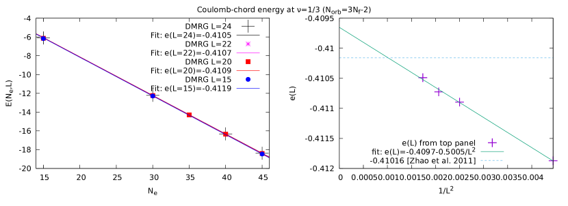
Figure 2: Energy at $\nu=1/3$ for the Coulomb-chord interaction potential. Left panel: energy as a function of $N_{e}$ for a few values of the circumference $L$ from 15 to 24. In all calculations the number of orbitals is $N_{\rm orb}=N_{\phi}+1=3N_{e}-2$. These energies are well fitted by : $E(N_{e},L)\simeq e(L)N_{e}+b(L)$, where $b$ can be interpreted as a contribution coming from the edge regions of the cylinder. Right panel: Extrapolation of $e(L)$ (obtained in the left panel) to $L=\infty$. All the calculations have been performed with a maximum bond dimension of the order of 8000.

4.2 Energy with Coulomb-Yukawa

The energy data at $\nu=1/3$ with the Coulomb-Yukawa interaction ($\exp(-\mu r)/r$) are plotted in Fig. 3 as a function of $N_{e}$ for a few values of $\mu$ between $10^{-3}$ and $0.3$. Here the circumference is fixed to $L=20$. The upper panel shows that energy $E(N_{e},\mu)$ is approximately linear in the number of particles (and thus in $L_{x}$ too), which allows to extract an energy per particle $e(\mu)$. So far the energy takes into account the electron-electron interaction, electron-background potential, and background-background energy. What is however missing is the energy due to the Coulomb interaction between each electron and its own periodic images (see Eq. 9). This contributes to the energy by a constant $e_{P}$ per particle which diverges logarithmically when $\mu\to 0$ :

$$e_{P}=\sum_{n=1}^{\infty}\frac{e^{-\mu nL}}{nL}=\frac{1}{L}\ln\left(1-e^{-\mu L}\right).$$ (27)

Adding $e_{P}$ to the extrapolated DMRG energies gives the data plotted in the bottom panel of Fig. 3. The corrected energy is extrapolated to $e_{0}\simeq-0.4097$ in the limit $\mu\to 0$. This is again in agreement with the previous estimates.

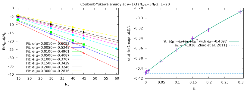
Figure 3: Energy at $\nu=1/3$ for the Coulomb-Yukawa interaction potential. Left panel: energy as a function of $N_{e}$ for a few values of $\mu$ and fixed $L=20$.

4.3 Orbital occupancies

With faith in the convergence of DMRG we now investigate the physical properties of the incompressible states. In Fig. (4) we display the occupation numbers of the Laughlin state obtained by finding the ground state of the $V_{1}$ model and the ground state of the Coulomb-Yukawa model for the same number of electrons/orbitals. We see that there are strong boundary effects near the physical end of the cylinder but they are quickly damped when one enters the bulk of the system. There is a wide region with uniform occupation that should capture the bulk physics at this filling factor. When we increase the number particles we observe that the regions of oscillating behavior are more and more far apart, increasing the range of the region whose behavior is that of the bulk. In the right panel of Fig. (4) we have removed one orbital from the cylinder, an operation that creates a quasielectron on top of the $\nu=1/3$ liquid. Indeed we observe in the center of the cylinder the appearance of a crater-like density modulation which is consistent with what we know about such quasiparticles. As a reference we have also plotted the occupation for the fiducial Laughlin state. The quasielectron is indeed localized in real space with an extent of the order of a few magnetic lengths.

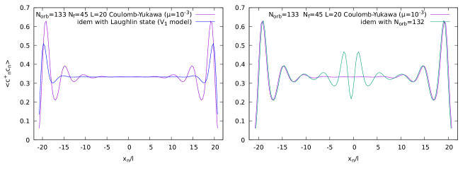
Figure 4: Left: Laughlin state occupation numbers in blue compared to Coulomb ground state from Yukawa potential with $\mu=10^{-3}$. Right: creation of one quasielectron by removal of one orbital state.

4.4 Wigner crystal

We now turn to the fate of the electron system at very small filling factors [23]. It is known that the FQHE liquids compete with the electron solid called the Wigner crystal and at small filling factors the Wigner crystal is expected to become the ground state of the system. The pair correlation function is well suited to reveal the crystal state since it displays directly the spatial density modulation as we have seen in the example of the hard-core model in section (3). We have performed calculations for filling factor $\nu=1/9$ using a number of particles of up to $N_{e}=21$. To accommodate a triangular crystal in a finite cylinder it is more favorable to have a number of particles which is a multiple of 3. With the truncation in space along the $x$ direction and the finite extent in the $y$ direction on should adjust $L$ so that the aspect ratio of the cylinder does not frustrate the expected triangular-lattice pattern, and so that a clean crystal structure can be observed. Such a case is displayed for $N_{e}=21$ electrons in Fig. (5) where we show that use of chord or Yukawa interactions leads to the same kind of crystal state.

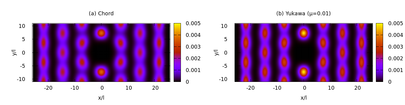
Figure 5: Pair correlation at $\nu=1/9$ for $N_{e}=21$ electrons and a cylinder with $L=22$. left panel is obtained with the chord distance regularization while the right panel is from Yukawa potential with $\mu=0.01$. The cylinder extent has been fine-tuned to maximize the appearance of the Wigner crystal state. In the chord and Yukawa cases the largest truncation weights are $\sim 3.10^{-9}$ and $\sim 10^{-9}$, for largest bond dimensions equal to $\sim 6900$ and $\sim 7600$ respectively.

5 Conclusions

Numerical techniques have been an invaluable tool in the understanding of the fractional quantum Hall effect. Even when severely size-limited they give an unbiased information about the ground state correlations and the nature of elementary excitations. The size limitation becomes problematic in several areas where rapid experimental progress challenge theoretical understanding. Notably this includes quantum Hall fractions with complicated commensurabilities like $4/11$ or $6/13$. This also severely hampers the understanding of multicomponent systems like graphene that involve a fourfold degeneracy of Landau levels due to spin and valley degrees of freedom. Multilayer systems made by stacking monolayer materials or fabricating on-purpose special devices are also a frontier where advances are needed. By looking at the Landau level problem from a one-dimensional point of view it is natural to use the DMRG algorithm with the obvious obstacle that interactions remain long-range in the physical regime. Indeed in the Hamiltonian Eq.(26) the decay factor governed by $\lambda=\exp(-2\pi^{2}/L^{2})$ is less and less effective as a cut-off on the range of interactions as we go to larger cylinders $L\rightarrow\infty$. When the range of interactions is large the so-called MPO representation of the Hamilotnian grows in complexity and the MPS bond dimensions also grows. So there is a trade-off also in DMRG involving all these parameters. We have presented a set of problems that have been studied following this path. We have seen that the present-day technology is advanced enough so that previously intractable problems in the FQHE realm can now be studied. For example there is no obvious obstacle to include the multicomponent nature of electrons in the near future.

We thank E. Burovsky and CSP organizers for invitation at CSP2020. One of us (ThJ) thanks Song-Yang Pu and Zheng-Wei Zuo for useful discussions. We also acknowledge CEA-DRF for computer time allocation on the supercomputer COBALT at CCRT.

References

References

- [1] White S R 1992 Phys. Rev. Lett. 69 2863–2866 URL http://link.aps.org/doi/10.1103/PhysRevLett.69.2863
- [2] Schollwöck U 2011 Annals of Physics 326 96 – 192 ISSN 0003-4916 URL http://www.sciencedirect.com/science/article/pii/S0003491610001752
- [3] Fishman M, White S R and Stoudenmire E M 2020 arXiv:2007.14822 [cond-mat, physics:physics] ArXiv: 2007.14822 URL http://arxiv.org/abs/2007.14822
- [4] Shibata N and Yoshioka D 2001 Phys. Rev. Lett. 86 5755–5758 URL https://link.aps.org/doi/10.1103/PhysRevLett.86.5755
- [5] Yoshioka D and Shibata N 2002 Physica E: Low-dimensional Systems and Nanostructures 12 43–45 ISSN 1386-9477 URL http://www.sciencedirect.com/science/article/pii/S138694770100306X
- [6] Shibata N and Yoshioka D 2003 J. Phys. Soc. Jpn. 72 664–672 ISSN 0031-9015 URL https://journals.jps.jp/doi/10.1143/JPSJ.72.664
- [7] Feiguin A E, Rezayi E, Nayak C and Das Sarma S 2008 Phys. Rev. Lett. 100 166803 URL https://link.aps.org/doi/10.1103/PhysRevLett.100.166803
- [8] Kovrizhin D L 2010 Phys. Rev. B 81 125130 URL https://link.aps.org/doi/10.1103/PhysRevB.81.125130
- [9] Zhao J, Sheng D N and Haldane F D M 2011 Phys. Rev. B 83 195135 URL https://link.aps.org/doi/10.1103/PhysRevB.83.195135
- [10] Zaletel M P, Mong R S K, Pollmann F and Rezayi E H 2015 Phys. Rev. B 91 045115 URL https://link.aps.org/doi/10.1103/PhysRevB.91.045115
- [11] Zhu W, Gong S, Haldane F and Sheng D 2015 Phys. Rev. Lett. 115 126805 URL https://link.aps.org/doi/10.1103/PhysRevLett.115.126805
- [12] Zhu W, Gong S S, Haldane F D M and Sheng D N 2015 Phys. Rev. B 92 165106 URL https://link.aps.org/doi/10.1103/PhysRevB.92.165106
- [13] Johri S, Papic Z, Schmitteckert P, Bhatt R N and Haldane F D M 2016 New J. Phys. 18 025011 ISSN 1367-2630 URL https://doi.org/10.1088%2F1367-2630%2F18%2F2%2F025011
- [14] Zhu W, Liu Z, Haldane F D M and Sheng D N 2016 Phys. Rev. B 94 245147 URL https://link.aps.org/doi/10.1103/PhysRevB.94.245147
- [15] Soulé P and Jolicoeur T 2012 Phys. Rev. B 85 155116 publisher: American Physical Society URL https://link.aps.org/doi/10.1103/PhysRevB.85.155116
- [16] Soulé P and Jolicoeur T 2012 Phys. Rev. B 86 115214 publisher: American Physical Society URL https://link.aps.org/doi/10.1103/PhysRevB.86.115214
- [17] Soulé P, Jolicoeur T and Lecheminant P 2013 Phys. Rev. B 88 235107 publisher: American Physical Society URL https://link.aps.org/doi/10.1103/PhysRevB.88.235107
- [18] Wójs A, Yi K S and Quinn J J 2004 Phys. Rev. B 69 205322 publisher: American Physical Society URL https://link.aps.org/doi/10.1103/PhysRevB.69.205322
- [19] Koulakov A A, Fogler M M and Shklovskii B I 1996 Phys. Rev. Lett. 76 499–502 publisher: American Physical Society URL https://link.aps.org/doi/10.1103/PhysRevLett.76.499
- [20] Fogler M M, Koulakov A A and Shklovskii B I 1996 Phys. Rev. B 54 1853–1871 publisher: American Physical Society URL https://link.aps.org/doi/10.1103/PhysRevB.54.1853
- [21] Fogler M M and Koulakov A A 1997 Phys. Rev. B 55 9326–9329 publisher: American Physical Society URL https://link.aps.org/doi/10.1103/PhysRevB.55.9326
- [22] Misguich G, Jolicoeur Th and Mizusaki T 2020 arXiv:1703.07095 [cond-mat] ArXiv: 1703.07095 URL http://arxiv.org/abs/1703.07095
- [23] Zuo Z W, Balram A C, Pu S, Zhao J, Jolicoeur Th, Wójs A and Jain J K 2020 Phys. Rev. B 102 075307 publisher: American Physical Society URL https://link.aps.org/doi/10.1103/PhysRevB.102.075307