Abstract

A painter is free to modify how components of a natural scene are depicted, which can lead to a perceptually convincing image of the distal world. This signals a major difference between photos and paintings: paintings are explicitly created for human perception. Studying these painterly depictions could be beneficial to a multidisciplinary audience. In this paper, we capture and explore the painterly depictions of materials to enable the study of depiction and perception of materials through the artists’ eye. We annotated a dataset of 19k paintings with 200k+ bounding boxes from which polygon segments were automatically extracted. Each bounding box was assigned a coarse label (e.g., fabric) and a fine-grained label (e.g., velvety, silky). We demonstrate the cross-disciplinary utility of our dataset by presenting novel findings across art history, human perception, and computer vision. Our experiments include analyzing the distribution of materials depicted in paintings, showing how painters create convincing depictions using a stylized approach, and demonstrating how paintings can be used to build more robust computer vision models. We conclude that our dataset of painterly material depictions is a rich source for gaining insights into the depiction and perception of materials across multiple disciplines. The MIP dataset is freely accessible at materialsinpaintings.tudelft.nl.

Introduction

Throughout art history, painters have invented numerous ways to transform the three-dimensional world onto flat surfaces [1, 2, 3, 4]. These transformations can be described by the geometry of the projection or in terms of two-dimensional drawing rules. Willats [5] noticed that for each projection there exists a set of drawing rules, but not vice versa. This illustrates an interesting and fundamental asymmetry that is characteristic to the visual perception of pictures: a depiction does not necessarily have to originate from a physically correct projection[6]. On one hand, this makes paintings unsuited as ecological stimulus [7]. On the other hand, as Gibson acknowledges, paintings are the result of endless visual experimentation, and therefore, indispensable for the study of visual perception.

In perception, distal refers to the outside world, while the related concept proximal refers to the projection of the distal world experienced on our senses i.e., the retinal image. The process of visual perception can be described as inferring properties of the distal stimulus from the available proximal information[8]. For example, perceived reflectance (lightness) is a distal property that is deduced from light on the retina (brightness) [9], or a distal circle is inferred from a proximal ellipse [10]. This is akin to ‘recovering intrinsic scene characteristics’ (which are distal) from images (which are proximal) in computer vision [11] .

A painter might work with ‘2D drawing rules’, but the goal usually is not to create an optically corrected projection, rather a painter strives to create a perceptually correct depiction. The artist does not copy a retinal image [12] (which would make the painter effectively a biological camera) but rather iteratively adapts templates until they ‘fit’ perceptual awareness [13]. In essence, a painting depicts the perceived distal world through a proximal stimuli.

The depiction and perception of pictorial space in paintings [5, 1, 2, 3, 4] has received much more attention than the depiction and perception of materials. As with the depiction of space, a painter is not concerned whether a material depiction is optically or physically correct. Instead, a painting is explicitly designed for human viewing and is only intended to be perceptually convincing. Human observers are able to visually categorize and identify depicted materials and material properties [14], despite a painting consisting only of paint and oils, similar to how we can perceive depth from a flat painting. Furthermore, for these painted materials, we can perceive distinct material properties such as glossiness, softness, transparency, etc [15, 16, 17]. A single material category (e.g., fabric) can display a large variety of these material properties, which demonstrates the enormous variation in visual appearance of materials. This variation in materials and material properties has received relatively little attention. In fact, the perceptual knowledge that is captured in the innumerable artworks throughout history can be thought of as the largest perceptual experiment in human history and it merits detailed exploration. The starting point for such an exploration is the creation of datasets that relate artworks to material perception. In this study, we introduce an accessible collection of material depictions in paintings, with which we hope to facilitate both perceptual, computational, and art historical research into materials.

A simple taxonomy of image datasets

In the current study we are primarily interested in the perception and depiction of materials and material properties [18, 19, 8, 14]. However, the use and creation of art-perception datasets is of broader interest. We propose a simple taxonomy of three image dataset usages: 1) perceptual, 2) ecological and, 3) computer vision usage. We expand on each of these three usages below and contextualize our dataset within this taxonomy.

Perceptual datasets.

To understand the human visual system, stimuli from perceptual datasets can be used in an attempt to relate the evoked perception to the visual input. We can roughly categorize three types of stimuli used for visual perception: natural, synthetic and manipulated. The first represent ‘normal’ images of objects, materials and scenes as they can be found in reality. Experimental design with such stimuli often attempts to relate the evoked perceptions to natural image statistics within the images or physical characteristics of the contents captured in the images. Some examples of uses of natural stimuli datasets include the memorability of pictures in general [20] or more specifically the memorability of faces [21]. In another example, images of natural, but novel objects were used to understand what underlies the visual classification of objects [22]. The second type, synthetic stimuli, are created artificially. Synthetic stimuli might represent the real world, but often contain image statistics that deviate greatly from natural image statistics. For example, [23] used a set of synthetic stimuli to test for memorability of data visualizations. Both natural and synthetic images can be manipulated, which leads to the third type of stimuli. Manipulated stimuli are often used to investigate the effect of image manipulations by comparing them to the original (natural or synthetic) image. Here the manipulations function as the independent variables. For example [24] created a database of images that contain scene inconsistencies that can be used to study the compositional rules of our visual environment. In another example, a stimulus set consisting of original and texture (i.e., manipulated) versions of animals found that perceived animal size is mediated by mid-level image statistics [25].

The advantage of using manipulated or synthetic images is that perceptual judgments can be compared to some independent variable, which is not available for natural images. Paintings are a special case: while they are being created they are a synthetic image that is rendered using oils and paints. However, when finished they are also real, physical objects. While retrieving the veridical data is impossible for almost all paintings, the advantage of using paintings is that it can often be seen, or (historically) inferred, how the painter created the illusory realism. Even if it can not be seen with the naked eye, chemical and physical analysis can be performed. In [17] a perceptually convincing depiction of grapes was recreated using a 17th century, explicitly written-down recipe. In the reconstruction, the depiction was created one layer at a time, each representing a separate and perceptually diagnostic image feature of the grape. In this way, paintings can give access to proximal information. Therefore, studying paintings in addition to more traditional stimuli like photos or renderings, can enrich our understanding of human perception. It should be noted that in this paper we focus on the image structure of the painting instead of the physical object. In other words, we focus on what is depicted within paintings and our data and analysis is limited to pictorial perception. In the remainder of this paper, when we mention paintings, we mean images of paintings.

Throughout history, painters have studied how to trigger the perceptual system and create convincing proximal depictions of complex distal properties of the world. This resulted in perceptual shortcuts, i.e., stylized depictions of complex properties of the distal world that trigger a robust perception. The steps and painterly techniques applied by a painter to create a perceptual shortcut can be thought of as a perception-based recipe. Following such a recipe results in a perceptual shortcut, which is a depiction that gives the visual system the required inputs to trigger a perception. Many of the successful depictions are now available in museum collections. As such, the creation of art throughout history can be seen as one massive perceptual experiment. Studying perceptual shortcuts in art, and understanding the cues, i.e., features required to trigger perceptions, can give insights into the visual system. We will demonstrate this idea by analyzing highlights in paintings and photos.

Ecological datasets.

To understand how the human visual system works it is important to understand what type of visual input is given by the environment. Visual ecology encompasses all the visual input and can be subdivided into natural and cultural ecology. Natural ecology reflects all which is found in the physical world. For example, to understand color-vision and cone cell sensitivities it is relevant to know the typical spectra of the environment. For this purpose, hyperspectral images [26, 27] can be used, in this case to investigate color metamers (perceptually identical colors that originate from different spectra) and illumination variation. In another example, a dataset of calibrated color images were used to understand color constancy [28] (the ability to discount for chromatic changes in illumination when inferring object color). The SYNS database was used to relate image statistics to physical statistics [29]. Another dataset contains photos taken in Botswana [30] in an area that supposedly reflects the environment of the proto-human and was used to investigate the evolution of the human visual system. Spatial statistics of today’s human visual ecology are clearly different from Botswana’s bushes as most people live in urban areas that are shaped by humans. For example, a dataset from [31] was used to compute the distribution of spatial orientations of natural scenes [32].

It is important to note that the majority of paintings in our dataset are painterly representations of the physical world around us that only loosely reflect the natural visual ecology, but strongly represent visual cultural ecology. They have influenced how people see and depict the world and have influenced visual conventions up to contemporary cinematography and photography. The recent surge in publicly available digitized art works, combined with the availability of advanced image analysis algorithms such as neural networks, has lead to a new branch of Art History: Digital Art History. Similar to the analysis of the human physical environment, Digital Art History concerns itself for example with the digitized analysis of artworks, artistic style [33] and beauty [34], or local pattern similarities between artworks [35].

Computer vision datasets.

Today, the majority of image datasets originate from research in computer vision. One of the first relatively large datasets representing object categories [36] has been used to both train and evaluate various computational strategies to solve visual object recognition. The ImageNet and CIFAR datasets [37, 38] are regarded to be standard image recognition datasets for the last decade of research ifn deep learning vision systems. Traditionally most visual research has been concerned with object classification but recently material perception has received increasing attention [39, 40, 41, 42].

Within vision science, paintings are considered as representing a special class of images, which deviate from natural photographs, as they are explicitly designed for viewing by humans [43]. The visual difference introduced by painterly depiction does not pose any significant difficulties to the human visual system, however it is more challenging for computer vision systems as a result of the domain shift [44, 45, 46]. Differences between painting images and photographic datasets include for instance composition, textural properties, colors and tone mapping, perspective, and style. As for composition, photos in image datasets are often ‘snapshots’, taken with not too much thought given to composition, and typically intended to quickly capture a scene or event. In contrast, paintings are artistically composed, and prone to historical style trends. Therefore, photos often contain much more composition variation relative to paintings. Within paintings, composition can vary greatly between different styles. The human visual system can distinguish styles – for example, Baroque vs. Impressionism – and also implicitly judge whether two paintings are stylistically similar. Research in style or artist classification, as well as neural networks that perform style transfer, attempt to model these stylistic variations in art [47, 48]. Humans can also discount stylistic differences, for example, identifying the same person or object depicted by different artists. Similarly, work in domain adaptation [44, 45, 46] focuses on understanding objects or stuff across different image styles.

Depending on the end goal for a computer vision system, it can be important to learn from paintings directly. When the end goal is to detect pedestrians for a self-driving car, learning from real photos, videos, or renderings of simulations can suffice. However, if the goal is to simulate general visual intelligence, multi-domain training sets seem essential. Furthermore, if the goal is to create computer vision systems with a perception that matches human vision, training on paintings could be very beneficial. Paintings are explicitly created by and for human perception and therefor contain all the required cues to trigger robust perceptions. Therefor, networks trained on paintings are implicitly trained on these perceptual cues.

The multifaceted nature of datasets.

While we have distinguished the broad purposes of datasets and exemplified each with representative datasets, it is important to keep in mind that these datasets can serve multiple goals across the taxonomy. For example, the Flickr Material Database [49] was initially created as a perceptual dataset to study how quickly human participants were capable of recognizing natural materials. However, since then it has also often been used as a computer vision dataset, including by the original authors themselves [50]. The dataset presented in this paper is explicitly designed with this multidisciplinary nature in mind.

Dataset collection and annotation

Our dataset consists of 19K paintings with crowd-sourced bounding box annotations over 15 material categories. We further distinguish these coarse material categories into over 50 fine-grained categories. Finally, we automatically extract polygon segments for each bounding box. The annotated dataset will be made publicly available. All paintings, bounding boxes, labels, and metadata are available at materialsinpaintings.tudelft.nl

The data collection was executed in multiple stages. Here we give an itemized overview of each stage and subsequently we discuss each stage in depth. The first two stages were conducted as part of a previous study [15], but we provide details here for completeness. Participants were recruited via Amazon Mechanical Turk (AMT). A total of 4451 unique AMT users participated in this study. Data collection was approved by the Human Research Committee of the Delft University of Technology and adheres to the Declaration of Helsinki.

1. First, we collected a large set of paintings.

2. Next, human observers on the AMT platform identified which coarse-grained materials they perceived to be present in each painting (e.g., “is there wood depicted in this painting?”).

3. Then, for paintings identified to contain a specific material, AMT users were tasked with creating a bounding box of that material in that painting.

4. Lastly, AMT users assigned a fine-grained material label to bounding boxes (e.g., processed wood, natural wood, etc.).

Collecting paintings

We collected 19,325 paintings from 9 online, open-access art galleries. The details of these art galleries are presented in Table 1. Images were downloaded from the online galleries, either using web scraping or through an API. For the majority of these paintings we also gathered the following metadata: title of the work, estimated year of creation and name of the artist.

For 92% of boxes, we also have an estimate of the year of production. These estimates were made by the galleries from which the paintings were downloaded. The distribution of the year of production for all paintings are plotted in Fig. 1, in bins of 20 years. Clearly, the data is not equally distributed over time. Museums, being cultural institutions, attempt to create a curated collection of art of cultural importance and not every year or time period is of equal cultural importance.

Gallery Name	Country	Count
The Rijksmuseum	Netherlands	4672
The Metropolitan Museum of Art	USA	3222
Nationalmuseum	Sweden	3077
Cleveland Museum of Art	USA	2217
National Gallery of Art	USA	2132
Museo Nacional del Prado	Spain	2032
The Art Institute of Chicago	USA	936
Mauritshuis	Netherlands	638
J. Paul Getty Museum	USA	399

Table 1: List of galleries, the country in which the museum is located, and the number of paintings downloaded from that gallery.

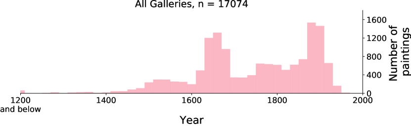
Fig 1: Histogram of the distribution of paintings over time. Each bin equals 20 years.

Image-level coarse-grained material labels

Next, we collected human annotations to identify material categories within paintings. We created a list of 15 material categories: animal, ceramic, fabric, sky, stone, flora, food, gem, wood, skin, glass, ground, liquid, paper, and metal. Our intention was to create a succinct list, that would nevertheless allow the majority of stuff within a painting to be annotated, and was partially based on [49, 51]. These categories primarily represent prototypical physical materials, as well as less typical, overarching categories that contain multiple materials such as food and animal. Note that we added the material category of skin directly, instead of a more overarching ‘human’ category as one might expect considering food and animal. We made this choice because of the scientific interest in the artistic depiction [52], perception [53, 54], and rendering of skin [55, 56]

In one AMT task, participants would be presented with 40 paintings at a time and one target material category. In the task, participants were asked if the painting depicted the target material (e.g., does this painting contain wood?). They could reply ‘Yes, the target material is depicted in this painting.’ by clicking the painting and inversely, by not clicking the painting, participants would reply with ‘No, the target material is not depicted in this painting.’. Each painting was presented to at least 5 participants for each of the 15 materials. If at least 80% of the responses per painting claimed that the material was depicted in the painting, we would register that material as present for that painting. In total, we collected 1,614,323 human responses in this stage from 3,233 unique AMT users participating.

Extreme click bounding boxes

In the previous stage, paintings were registered to depict or not to depict a material. However, that stage does not inform us (1) how often the material is depicted, nor (2) where the material(s) are within the painting.

We gathered this information on the basis of extreme click bounding boxes. For extreme click bounding boxes, a participant is asked to click on the 4 extreme positions of the material: the highest, lowest, most left-, and most right-wards point [57]. See Fig. 2 for an example. In the task, participants were presented with paintings that depicted the target material and tasked to create up to 5 extreme click bounding boxes for the target material.

To make bounding boxes within the task, the participants would use our interface, which allows users to zoom in and out, and pan around the image. The interface furthermore allowed participants to finely adjust the exact location of the extreme points by dragging the points around. Initially, the tasks were open to all AMT workers, but after around 2000 bounding boxes were created by 114 AMT users, with manual inspection, we found that the quality of bounding boxes varied greatly between participants. Therefore, we restricted the work to a smaller number of manually selected participants who were observed to create good bounding boxes. After this restriction, new boxes were manually inspected by the authors, and in a few cases additional participants were restricted due to a deterioration of bounding box quality. Simultaneously additional participants were granted access to our tasks after passing (paid) qualification tasks. As a result, the number of manually selected participants varied between 10 and 20 participants. In total, 227,810 bounding boxes were created by participants.

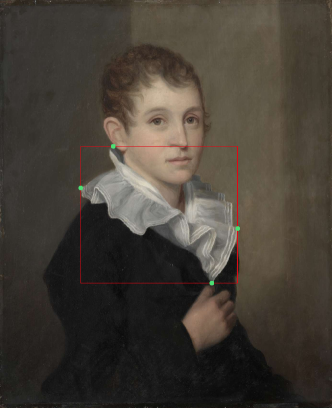
Fig 2: An example of four extreme clicks (marked in green) made by a user on a piece of fabric. These points correspond to the most left, most right, highest and lowest points on the annotated item. The red-line displays the resulting bounding box.

Automatic bounding boxes.

While we consider our dataset to be quite larger, it only covers a small but representative portion of art history. It might be required to access materials in paintings that are not part of our dataset. To allow for this, we have trained a FasterRCNN [58] bounding box detector to localize and label material boxes in unlabelled paintings. The model was finetuned from a model trained on COCO with the COCO hyperparameters from [59]. First we trained the detector on 90% of annotated paintings in the dataset. In section Automatically detected bounding boxes. below, we show our evaluation of the network, which was performed on the remaining 10% of annotated paintings. While we created this network to be able to detect paintings outside our dataset, we decided to apply the network on our dataset in order to more densely annotate our paintings. Therefor, after the evaluation, we ran the detection network on the entire set of paintings, i.e., training and testing data, in an attempt to more exhaustively annotate materials within paintings. From the automatic detected bounding boxes we first removed all boxes that scored $<$50% confidence (as calculated by FasterRCNN). Next, we filtered out automatic boxes that were likely already identified by human annotators, be removing automatic bounding boxes that scored $\geq{50}$% on intersection over union, i.e., automatic boxes that shared the majority of it’s content with human boxes. This resulted in an additional 96k bounding boxes, all of which are also available on materialsinpaintings.tudelft.nl.

Fine-grained labels

In this step we supplemented the previously collected material labels with fine-grained material labels (see Table 2). For example, a bounding box labelled as fabric could now be labelled as silk, velvet, fur, etc.. We excluded bounding boxes that were too small (e.g., width in pixels $\times$ height in pixels $\leq{5000}$) and boxes that were labelled as sky, ground or skin for which fine-grained categorizations were not annotated. We collected fine-grained labels for the remaining 150,693 bounding boxes. Note that this only concerns the bounding boxes created by human annotations as no automatically detected boxes were assigned a fine-grained material label. For each of these 150,693 bounding boxes, we gathered responses from 5 different participants. If the 5 responses reached an agreement of at least 70%, we would assign the agreed upon label to the bounding box. To guide the workers, we provide a textual description for each fine-grained category for them to reference during the task. We did not provide visual exemplars as we did not want to bias the workers into template matching instead of relying on their own perceptual understanding.

We found that it is non-trivial to define fine-grained labels in such a way that they are concise, uniform and versatile (i.e., useful across different scientific domains) while still being recognizable and/or categorizable by naive observers. We applied the following reasoning to select fine-grained labels: first, we tried to divide the materials into an exhaustive list with as few fine-grained labels as possible. For example, for ‘wood’, each bounding box is either ‘processed wood’ or ‘natural wood’. If an exhaustive list would become too long to be useful, we would include an ‘other’ option. For example, for ‘glass’ we hypothesized that the vast majority of bounding boxes would be captured by either ‘glass windows’ or ‘glass containers’. However, to include all possible edge cases such as glass spectacles and glass eyeballs, we included the ‘other’ option.

A possible subset for ‘metal’ we considered was ‘iron’,‘bronze’, ‘copper’, ‘silver’, ‘gold’ , ‘other’. However, we feared that naive participants would not be able to consistently categorize these metals. An alternative would be to subcategorize on object-level, e.g. ’swords’, ’nails’, etc., but as we are interested in material categorization, we tried to avoid this as much as possible. Thus, for ‘metal’, and for the same reason ‘ceramic’, we required a different method. We chose to subcategorize on color, as often the color for these materials are tied to object identity.

Participants are shown one bounding box at a time and are instructed to choose which of the fine-grained labels they considered most applicable. Additionally, they are able to select a ‘not target material’ option.

We collected over one million responses from 1114 participants. This resulted in a a total of 105,708 boxes assigned with a fine-grained label. See Table 2 for the numbers per category.

Results and applications

We conducted a diverse set of experiments to demonstrate how our annotated art-perception dataset can drive research across perception, art history, and computer vision. First, we report simple dataset statistics. Next, we organized our findings under the proposed dataset usage taxonomy: perceptual applications, ecological applications and computer vision applications.

Dataset statistics

The final dataset contains painterly depictions of materials, with a total of 19,325 paintings. Participants have created a total of 227,810 bounding boxes and we additionally detected 96k using a FasterRCNN. Each box has a coarse material label and 105,708 also have been assigned a fine-grained material label. The total number of instances per material categories (coarse- and fine-grained) can be found in Table 2. Further analysis of spatial distribution of categories, co-occurences, and other related statistics will be discussed in a following section in the context of visual ecology.

Coarse-grained	Fine-grained	# Labels
animal		11606
	birds	1822
	reptiles and amphibians	144
	fish and aquatic life	289
	mammals	7752
	insects	155
	other animals	10
ceramic		3641
	brown or red	1088
	white	381
	decorated	289
	other ceramic	14
fabric		31557
	velvety	261
	lace	491
	silky/satiny	1354
	cotton/wool-like	5712
	brocade	96
	fur	27
	other fabric	12
flora		26693
	trees	12851
	vegetables	96
	fruits	1238
	flowers	2515
	plants	3699
food		3690
	cheese	11
	vegetables	107
	fruits	1536
	meat or poultry	183
	bread	127
	seafood	183
	nuts	8
	other	14
gem		10525
	pearls	719
	gemstones	715
	other gems	1
glass		5546
	glass window	2243
	glass container	1003
	other glass	171
ground		2552
liquid		5737
	body of water	4583
	liquid in container	458
	other liquid	172
metal		27708
	colorless metal	2933
	yellowish metal	4435
	brownish or reddish metal	510
	multicolored or other colored metal	215
paper		3167
	paper book	1380
	paper sheets	585
	paper scrolls	114
	other paper	19
skin		32323
sky		12734
stone		23157
	processed stone	9226
	natural stone	9429
wood		26953
	processed wood	12810
	natural wood	10751

Table 2: The number of annotated bounding boxes for each coarse- and fine-grained category. Note that not every bounding box is associated with a fine-grained label since participants were not always able to arrive at a consensus. See main text for details.

Perceptual applications

We believe that the materials in this dataset can be useful as stimuli for perceptual experiments. We demonstrate this in this section by performing an annotation experiment to study perception-based recipes.

Perception-based recipes in painterly depictions

As previously argued, we believe that painterly techniques are a sort of perception-based recipe. Applying these recipes results in a stylized depiction that can trigger a robust perception of the distal world. Studying the image features in paintings can lead to an understanding of what cues the visual systems needs to trigger a robust perception.

Here we explore a perceptual shortcut for the perceptions of glass by annotating highlights in paintings and comparing these with highlights in photos. For input stimuli, we use bounding boxes from our dataset and photographs sourced from COCO [60]. Participants for this study included 3 of the authors, and one naive lab-member.

Stimuli.

We used 110 images of drinking glasses. First, we selected all bounding boxes in the glass, liquid container category in our dataset. From this set, we manually selected drinking glasses, since this category can also contain items such as glass flower vases. Next, we removed all glasses that were most occluded, were difficult to parse from the background - for example when multiple glasses were standing behind each other, and removed images smaller then 300x300 pixels. This resulted in a few hundred painted drinking glasses.

Next, we downloaded all images containing cups and wineglasses from the COCO [60] dataset, from which we removed all non-glass cups, occluded glasses, blurry glasses and glasses that only occupy a small portion of the image, and small images. This left us with 55 photos of glass cups and wineglass. Next, we randomly selected 55 segmentations from our painted glass collection. Each stimulus was presented in the task at 650 $\times$ 650 pixels, keeping aspect ratio intact.

During this selection phase, we did not base our decision on the shape of the glass. After the experiment, as part of the analysis, we divided the glasses into three shapes, namely spherical, cylindrical, and conical glasses. See Fig. 3 for an example of each shape.

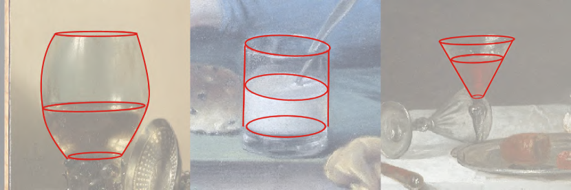
Fig 3: Examples of the three glass shapes. From left to right: spherical, cylindrical and conical. The red geometry annotations were manually created by the authors, and were used to standardize across glasses for the highlight analysis.

Task.

Participants annotated highlights on drinking glasses using an annotation interface. In the annotation interface, users would be presented with an image on which the annotated geometry was visible. This made it clear which glass should be annotated, in case multiple glasses were visible in the image. Users were instructed to instruct all visible highlights on that glass. Once the user started annotating highlights, the geometry would no longer be visible. Annotations could be made by simply holding down the left-mouse button and drawing on top of the image. Once a highlight was annotated a user could mark it as finished and continue with the next highlight, and eventually move to the next image.

Results.

To compare the highlights between photos and stimuli, we resized each glass to have the same maximum width and height, and then overlaid each stimuli on the center. When all 110 stimuli are overlaid (not visualized) the resulting figure is appears noisy. However, when we split the stimuli on media and shape, a clear pattern emerges for painted stimuli Fig. 4.

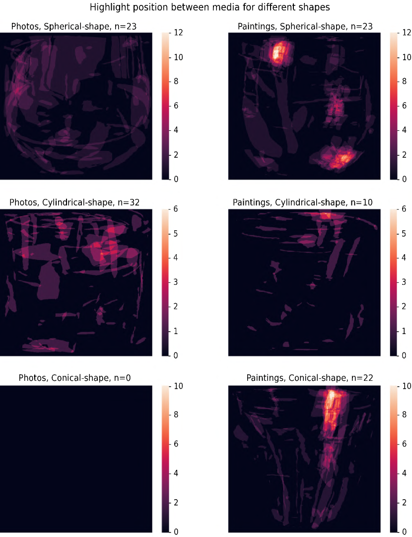
Fig 4: The overlaid highlights created by users, split on media and glass shape. In general, the photographic glass shapes display more variability and do not display a clear pattern. Note that for photos, no stimuli existed with a conical shape in our set which leads to a black image, since there were no highlight-annotations. On the right, for painted glasses, we see clear patterns in the placement of highlights for each glass shape.

As can be seen, painters are more likely to depict highlights on glasses adhering to a stylized pattern, at least for spherical and conical glasses. This pattern of highlights is perceptually convincing, but is perhaps surprisingly uniform in comparison with the variation found within reality. Furthermore, we calculated the agreement between each pair of participants,as the ratio of pixels annotated by both participants (i.e., overlapping area) divided by the number of pixels that was an annotated by either participant (i.e., total area). Averaged across participants, the agreement on paintings (0.33) was around 50% higher relative to the average agreement between participants on photos (0.21). This means that for our stimuli, highlights in paintings are less ambiguous when compared to photos.

Ecological applications

The ecology displayed within paintings are representative of our visual culture. Our dataset consists of paintings spanning 500+ years of art history. This provides a unique opportunity to analyze a specific sub-domain of visual culture, i.e., that of paintings. We first analyze the presence of materials in paintings in the Material presence section and in the next section we analyse this over time. In The spatial layout of materials , we visualize the spatial distributions of materials in our dataset. In the last section, we analyze the automatically detected bounding boxes.

Material presence.

Within the 19,325 paintings, participants exhaustively identified the presence of 123,244 instances of 15 coarse materials. In other words, for each painting, participants indicated if each material is or is not present. The distribution of unique materials per painting is normally distributed with an average of 5.7 unique coarse materials present per painting (std = 2.8 materials). The most frequent materials are skin and fabric. The least frequent are ceramics and food. The relative frequency of each coarse material is presented in Fig. 5. We did not exhaustively identify fine-grained materials within paintings, so we will not report those statistics here.

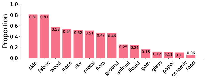
Fig 5: The proportion of paintings in our dataset that depict at least one instance of each material.

Based on prior knowledge of natural ecology, one might assume that some materials, such as skin and fabric might often be depicted together in paintings. To quantify the extent to which materials are depicted together, we create a co-occurrence matrix presented in Fig. 6, where each cell is the co-occurrence for each pair of materials as the number of paintings where both materials are present, divided by the number of paintings where either (but not both) materials are present. We can see for example, that if skin is depicted, there is a 94% change to also find fabric in the same painting.

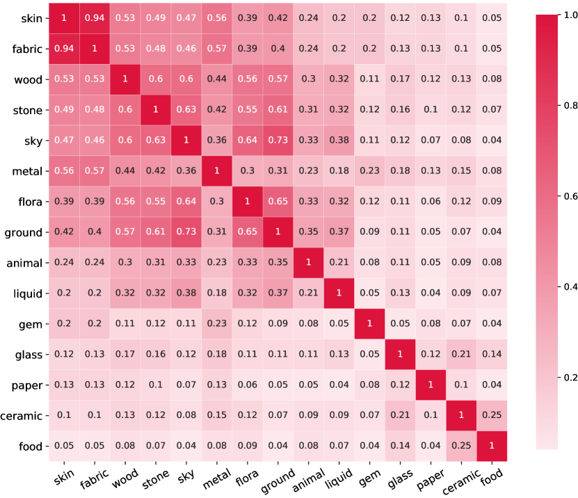
Fig 6: Co-occurrence matrix. Each cell equals the number of paintings where both materials are present divided by the number of paintings where one or the other material is present.

Furthermore, one might expect that the presence of one material can have an influence on another material. For example, one might expect that gem might almost always be depicted with skin, but that skin is only sometimes depicted with gem. To quantify these relations, we calculated the occurrence of a material given that another material is present. We visualize this in Fig. 7. Here we see that if gem is present, then skin is found in 99% of the paintings, but that if skin is present, then gem is found in only 20% of the paintings. The same relationship is true for gem and fabric. This implies that gems are almost always depicted with human figures, however that human figures are not always shown with gems. Another example, when liquid is present, in 85% of the paintings, wood is also present. One might be reminded of typical naval scenes, or landscapes with forests and rivers. Inversely, when wood is present, only 34% of the paintings depict liquid. For food and ceramics, two materials which are present in less then 10% of paintings, we see that if food is present, ceramics has a 53% change to be present as well, but the inverse is only 33%. This implies that food is served in, or with, ceramic containers half of the time, but that this is only 1/3rd of what ceramics is used for.

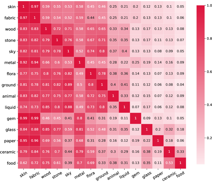
Fig 7: Likelihood matrix. This matrix visualizes the influence a material has on the likelihood of finding another material within the same painting, i.e., if one material on the y-axis is present, then how does this impact the presence of other materials on the x-axis? Calculated as the number of paintings where both materials are present, divided by the number of paintings that contain only one of the materials.

Material presence over time.

We have previously shown the distributions of materials in paintings in Fig. 5. When we created similar distributions (not visualised) for temporal cross-sections, for example for a single century, we found that these distributions were remarkably similar to the average distribution in Fig. 5. We used t-tests, to see if the distribution for any century was significantly different from the average distribution in Fig. 5 and found no significant effect. This means that despite the changes in stylistic and artistic techniques over time, the distribution of materials (such as in Fig. 5 remained remarkably stable over time for the period covered in our dataset.

The spatial layout of materials.

Paintings are carefully constructed scenes and it follows that a painter would carefully choose the location at which to depict a material. For example, [61] reported a strong spatial convention to center one eye within portraits. With the knowledge that spatial conventions exists within paintings, it makes sense to assume these might extend to materials. The average spatial location and extent of materials is visualized by taking the (normalized) location of each bounding box for a specific material and subsequently plotting each box as a semi-transparent rectangle. The result is a material heatmap, where the brightness of any pixel indicates the likelihood to find a material at that pixel. In this section, we limit the material heatmaps to only include the bounding boxes created by human annotators. In the next section, we visualize the material heatmaps for automated boxes too.

Material heatmaps for the 15 coarse materials are shown in Fig. 8. The expected finding that sky and ground are spatially high and low within images serves as a simple validation or sanity-check of the data. It is interesting to see how skin and gem are both vertically centered within the canvas. It appears to suggests a face, with necklaces and jewelry adorning the figure. In general, each material heatmap appears to be roughly vertically symmetric. For glass, there does however appear to be a minor shift towards the top-left. This might be related to an artistic convention, namely that light in paintings usually comes from a top-left window [62]. When we look at the heatmaps for the sub-categories for glass in Fig. 9, we see that it is indeed glass windows that show the strongest top-left bias.

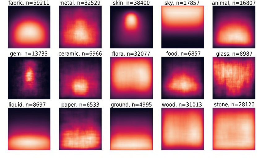
Fig 8: Material heatmaps, which illustrate the likelihood at any given pixel to find the target material at that pixel. Brighter colors indicate higher likelihoods.

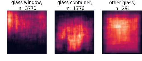
Fig 9: Material heatmaps for glass sub categories. For glass windows, it is interesting to see the clustering in the top-left corner, which is in agreement with the artistic convention of having light come from the top left.

Automatically detected bounding boxes.

Besides the bounding boxes created by humans, we also trained a FasterRCNN network to automatically detect bounding boxes with 90% of the data as training data. On the remaining unseen 10% of paintings, the network detected 90,169 bounding boxes. We removed those with a confidence score below 50%, which resulted in 24,566 remaining bounding boxes. In the section below, all references to the automated bounding boxes refer to these 24,566 bounding boxes.

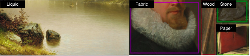
Fig 10: Examples of detected materials in unlabeled paintings. Automatically detecting materials can be useful for content retrieval for digital art history and for filtering online galleries by viewer interests.

A qualitative sample of detected bounding boxes is given in Fig. 10. Our human bounding boxes are non-spatially exhaustive in nature meaning that not every possible material has been annotated. As a result, the automatically created bounding boxes can not always be matched against our human annotations and thus we can not use this to evaluate their quality. In order to validate the automatic bounding box detection, we performed a simple user study to get an estimate of the accuracy per material class, which is visualized in Fig. 11. In the user study, a total of 50 AMT participants judged a random sample of 1500 bounding boxes. The bounding boxes were divided into 10 sets of 150 stimuli, each set contain 10 boxes per course material class. Each individual participant only saw one set, and each set was seen by 5 unique participants. The order of stimuli was randomized between sets and participants. A participant was instructed to rate each stimuli was either a good or a bad bounding box. This leads to a total of 7500 votes, 500 per material classes. The ratio of good to bad votes per material classes can serve as a measure of accuracy, which has been visualized in Fig. 11.

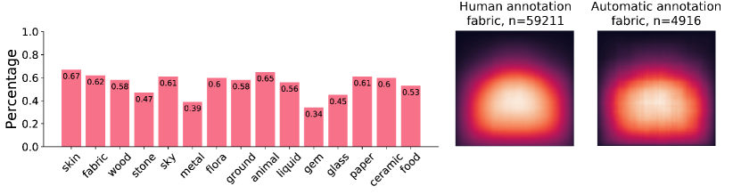
Fig 11: In the bar graph, the accuracy for automatically detected bounding boxes is displayed in the same order as in Fig. 5. The values were derived from human quality votes. On the right, we compare the material heatmaps for fabric between the automated and the human annotation bounding boxes.

As a result of the user study, we found a mean average accuracy of 0.55. While not high, these results are somewhat interesting in that they show that a FasterRCNN model is capable of detecting materials in paintings, without any changes to the network architecture or training hyperparameters. It is certainly promising to see that an algorithm designed for object localization in natural images can be readily applied to material localization in paintings. Likely, the accuracy could be further improved by finetuning the network which we have not done in this paper.

It is interesting to note that the spatial distribution of automatically detected bounding boxes looks very similar to the spatial distribution of the human annotated bounding boxes. We have visualized the material heatmap for one material, fabric, for the automated bounding boxes to show the similarity with the material heatmap for the same material created from human annotation bounding boxes. This has been visualized in the right side of Fig. 11

Computer vision applications

In this section, we will first apply existing segmentation tools designed for natural photographs to extract polygon segmentations. Next, we perform an experiment to demonstrate the utility of paintings for automated material classification.

Extracting polygon segmentations

A natural extension of material bounding boxes is material segments [40, 41, 42]. Polygon segmentations are useful for reasoning about boundary relationships between different semantic regions of an image, as well as the shape of the regions themselves. However, annotating segmentations is expensive and many modern datasets rely on expensive manual annotation methods [40, 60, 63, 42, 64]. Recent work has focused on more cost effective annotation methods (e.g. [65, 66, 67, 68]). One broad family of methods to relax the difficulty of annotating polygon segmentations is through the use of interactive segmentation methods that transform sparse user inputs into a full polygon masks.

For this dataset, we apply interactive segmentation with the crowdsourced extreme clicks as input. To evaluate quality, we compared against  4.5k high-quality human annotated segmentations from [15], which were sourced from the same set of paintings. We find that both image-based approaches like GrabCut (GC) [69] and modern deep learning approaches such as DEXTR [66] perform well. Surprisingly, DEXTR transfers quite well to paintings despite being trained only on natural photographs of objects. The performance is summarized in Table 3. The performance is summarized using the standard intersection over union (IOU) metric. IOU is computed as the intersection between a predicted segment and the ground truth segment divided by the union of both segments. IOU is computed for each class, and mIOU is the mean IOU over all of the classes. Samples are visualized in Fig. 12. Segments produced by these methods from our crowdsourced extreme points will be released with the dataset.

mIOU (%)
​​Grabcut​​ ​​Rectangle​​ ​​Grabcut​​ ​​Extr​​ ​​DEXTR​​ ​​Pascal-SBD​​ ​​DEXTR​​ ​​COCO​​ ​​DEXTR​​ ​​Finetune​​ 44.1 72.4 74.3 76.4 78.4
DEXTR Finetune IOU By Class (%)
Animal Ceramic Fabric Flora Food 76.9 86.8 79.1 77.0 87.5 Gem Glass Ground Liquid Metal 74.4 83.2 69.6 73.0 75.5 Paper Skin Sky Stone Wood 86.1 78.9 78.5 81.7 67.4

Table 3: Segmentations from extreme clicks. Grabcut [69] rectangles use bounding-box only initialization as a reference baseline. Grabcut Extr is based on the improved GC initialization from [57] with small modifications: (a) we compute the minimum cost boundary with the cost as the negative log probability of a pixel belonging to an edge; (b) in addition to clamping the morphological skeleton, we also clamp the extreme points centroid as well as the extreme points; (c) we compute the GC directly on the RGB image. DEXTR [66] Pascal-SBD and COCO are pretrained DEXTR ResNet101 models on the respective datasets. Note that Pascal-SBD and COCO are natural image datasets of objects, but DEXTR transfers surprisingly well across both visual domains (paintings vs. photos) and annotation categories (materials vs. objects).

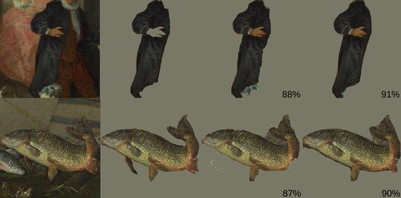
Fig 12: Segmentation visualizations. Left to right: Original Image, Ground Truth Segment, Grabcut Extr Segment, DEXTR COCO Segment. Both Grabcut and DEXTR use extreme points as input. For evaluation, the extreme points are generated synthetically from the ground truth segments. The IOU for each segmentation is shown in the bottom right corner.

Learning Robust Cues for Finegrained Fabric Classification

The task of distinguishing between images of different semantic content is a standard recognition task for computer vision systems. Increasing attention is being given to “fine-grained” classification where a model is tasked with distinguishing images of the same broad category (e.g., distinguishing different species of birds or different types of flora [70, 71, 72]). Fine-grained classification is particularly challenging for deep learning systems. Such a task depends on recognizing specific attributes for each finegrained class; in comparison, classifiers can perform well on coarse-grained classification by relying on context alone. We hypothesize that the painted depictions of materials can be beneficial for this task. Since some artistic depictions focus on salient cues for perception through perceptual shortcuts, it is possible that a network trained on paintings is able to learn a more robust feature representation by focusing on these cues.

Task.

We experimented with the task of classifying cotton/wool versus silk/satin. The latter can be recognized through local cues such as highlights on the cloth; such cues are carefully placed by artists in paintings. To understand whether artistic depictions of fabric allow a neural network to learn better features for classification, we trained a model with either photographs or paintings. High resolution photographs of cotton/wool and silk/satin fabric and clothing (dresses, shirts) were downloaded and manually filtered from publicly available photos licensed under the Creative Commons from Flickr. In total, we downloaded roughly 1K photos. We sampled cotton/wool and silk/satin samples from our dataset to form a corresponding dataset of 1K paintings. We analyzed the robustness of the classifier trained on paintings versus the classifier trained on photos in two experiments below. Taken together, our results provide evidence that a classifier trained on paintings can be more robust than a classifier trained on photographs.

Generalizability of classifiers.

Does training with paintings improve the generalizability of classifiers? To test cross-domain generalization, we test the classifier on types of images that it has not seen before. A classifier that has learned more robust features will perform better on this task than one that has learned to classify images based on more spurious correlations. We tested the trained classifiers on both photographs and paintings.

In Table 4, the performance of the two classifiers are summarized. We found that both classifiers perform similarly well on the domain they are trained on. However, when the classifiers are tested on cross-domain data, we found that the painting-trained classifier performs better than the photo-trained classifier. This suggests that the classifier trained on paintings has learned a more generalizable feature representation for this task.

Human agreement with classifier cues.

How indicative are the cues used by each classifier to humans? We produced evidence heatmaps with GradCAM [73] from the feature maps in the network before the fully connected classification layer. We extracted high resolution feature maps from images of size 1024 $\times$ 1024 (for a feature map of size 32 $\times$ 32). The heatmaps produced by GradCAM show which regions of an image the classifier uses as evidence for a specific class. If the cues (i.e., evidence heatmaps, such as in Fig. 13) are clearly interpretable, this would imply the classifier has learned a good representation. For both models, we computed heatmaps for test images corresponding to their ground truth label. We conducted a user study on Amazon Mechanical Turk to find which heatmaps are judged by human to be more informative. Users were shown images with regions corresponding to heatmap values that are above 1.5 standard deviations above the mean. Fig. 13 illustrates an example. Users were instructed to ’select the image that contains the regions that look the most like ¡material¿’, where ¡material¿ was either cotton/wool or silk/satin. We collected responses from 85 participants, 57 of which were analyzed after quality control. For quality control, we only kept results from participants who spent over 1 second on average per trial.

Overall, we found that the classifier trained on paintings uses evidence that is better aligned with evidence preferred by humans (Fig. 14). Due to domain shifts when applying classifiers to out-of-domain images, we would expect the cues selected by the painting classifier to be preferable on paintings, and the cues selected by the photo classifier to be preferable on photos. Interestingly, this does not hold for photos of satin/silk (see last column of Fig. 14) – found that users have no preference for the cues from either classifier, i.e., the cues from the painting classifier appears to be equally informative as the cues from the photo classifier for categorizing silk/satin in photos. This suggests that either (a) the painting classifier has learned the “key” human-interpretable cues for recognizing satin/silk, or (b) that the photo classifier has learned to classify satin/silk based on some spurious contextual signals that are difficult to interpret by humans. We asked users to elucidate their reasoning when choosing which set of cues they preferred. In general, users noted that they preferred the network which picks out regions containing the target class. Therefore, it seems that the network trained on paintings has learned better to distinguish fabric through the appearance of such fabrics in the image over other contextual signals (see Fig. 13).

Fig 13: Visualization of cues used by classifiers. Left to right: Original Image, Masked Image (Painting Classifier), Masked Image (Photo Classifier). The unmasked regions represent evidence used by the classifiers for predicting “silk/satin” in this particular image. See main text for details.

	Photo $\rightarrow$ Photo	Painting$\rightarrow$ Painting
MEAN F1 Score	79.6%	80.5%
	Photo $\rightarrow$ Painting	Painting$\rightarrow$ Photo
MEAN F1 Score	49.5%	57.8%

Table 4: Classifier performance across domains. Classifiers are trained to distinguish cotton/wool from silk/satin. The first column represents the classifier trained on photographs, and the second column represents the classifier trained on paintings. In the first row, the classifiers are tested on images of the same type they were trained on (i.e., trained and tested on photos, and trained and tested on paintings). In the second row, the classifiers are tested on the other medium, i.e., trained on photos and tested on paintings and vice versa.

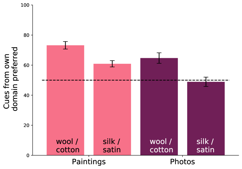
Fig 14: Human preference for classification cues used by each classifier. The y-axis represents how often humans prefer the cues from a classifier trained on the same domain as the test images. For example, the first bar indicates that in 73.2% of the cases, humans preferred cues from the classifier trained on paintings when classifying wool/cotton paintings (and thus, the inverse, that in 26.8% of the cases, humans preferred cues from the photo classifier.) Interestingly, note the last column – humans equally prefer cues used by both classifiers for classifying silk/satin photos despite the painting classifier never seeing a photo during training.

Discussion and conclusion

In this paper, we presented the Materials in Paintings (MIP) dataset – a dataset of painterly depictions of different materials throughout time. The dataset can be visited, browsed and downloaded at materialsinpaintings.tudelft.nl.

The MIP dataset consists of 19,325 high resolution images of painting, in which we have annotated material information. Various datasets exists that contain artworks, for example, the Painting-91 dataset from [74] consists of around 4000 paintings from 91 artists and was introduced for the purpose of categorization on style or artist. More recently, Art500k was released, which contains more than 500k low resolution artworks which were used to automatically learn to identify content and style [75] in paintings. Object recognition, while much more popular on natural photographs, also has been performed on paintings such as in [76] and [77]. It is worth mentioning the WikiArt dataset, which is created by a non-profit organisation, with the admirable goal “to make world’s art accessible to anyone and anywhere” [78]. The WikiArt dataset has been widely used for a variety of scientific purposes [79, 80, 47, 81, 82].

What makes the MIP dataset unique is the availability of information on material depiction. To our knowledge, no datasets exist that provide annotations on material depictions in paintings, however a few datasets exists that provide material information for natural images. A notable example is OpenSurfaces [40], which contains around 70k crowd-sourced polygon segmentations of materials in photos. The Material In Context database improved on OpenSurfaces by providing 3 million samples across 23 material classes [41].

The availability of materials in paintings is beneficial to the research of material depiction and perception. In contemporary material perception (see [83] for a review) paintings are rarely used. A few noteworthy exceptions have already been mentioned within this paper, such as the work of Di Cicco [17] in which the authors studied the depiction of grapes in 17th century and used an explicit recipe written by a 17th century painter to recreate painterly depictions of grapes. An explicit, written-down recipe is not required for perceptual research as we have shown with our annotated highlights on glass. By only annotating pictorial cues the perception-based recipe can be revealed. Our findings raise an interesting question: what other perception-based recipes could generate insights into material perception? Does our finding of stylized highlights on glasses extend to other shiny materials? Within material perception, the perception of glossiness has received much attention [84, 85, 86, 87], and a better understanding of painterly depiction of glossy materials could be very beneficial. Of course, there is no reason why perception-based recipes should be limited to glass or glossiness, as painterly depictions are capable of conveying robust perceptions for many more perceptual attributes and materials [15]

For art history, the ability to easily access a large number of paintings that depict a material might be interesting. Crowley and Zisserman [88] pointed out that art historians often have the unenviable task of finding paintings for study manually. With the release of MIP, this task might now become slightly easier for art historians that study the artistic depiction of materials, such as for example stone [89, 90]. The fabric category, and it’s fine-grained subclasses such as velvet, silk and lace could be used for the study of fashion and clothes in paintings in general [91, 92], for paintings from a specific cultural context, such as Italian [93], English and French [94] or even for the clothes worn by specific artists [95]. The human body and it’s skin, which clothing covers, is often studied within paintings [91, 96, 52]. For example, the Metropolitan Museum, published an essay on anatomy in the Renaissance, for which artworks depicting the human nude were used, many of which are incorporated in MIP [97]. In this work on anatomy, only items from the Metropolitan Museum were used but with the MIP this could be extended and compared to other museum collections. Furthermore, through for example the food and flora category, the MIP could give access to typical artistic scenes such as stillives [98, 99] and floral scenes [100] respectively.

The usages of large sets of images has been a common practice for computer vision research. The usage of art datasets has been less common, but paintings have nevertheless been used in various ways. Models that learn to convert photographs into painting-like or sketch-like images have been studied extensively for their application as a tool for digital artists [48]. Recent work has shown that such neural style transfer algorithms can also produce images that are useful for training robust neural networks [101]. In a related paper, we more explicitly discuss specific applications of the MIP dataset for computer vision [102]. Similarly, other domains of computer vision research might benefit from painterly depictions. The finding of our perception-based recipe for the stereotypical depiction of highlights on glasses could be useful for the generation of images. Current image generation algorithms are capable of generating novel images, based on learned statistics from a dataset [103, 104]. While a specific category of generated images, e.g., faces, [105] is rapidly becoming indistinguishable from reality, a larger set of categories is still proving difficult to generate due to the lack of sufficient training data. Moreover, it would be interesting to see if applying explicit painterly techniques, e.g., perceptual shortcuts, or stereotypical depictions could be leveraged in image generation. Perceptual shortcuts do not mimic the statistics of the real world, but instead capture image cues in a stylized depiction that explicitly trigger convincing human perceptions. Image generation algorithms that learn to use perceptual shortcuts might more efficiently capture image features that trigger perceptions.

Although the findings reported in this study are valuable for their own sake, we hope that the MIP dataset can support research in multiple disciplines, as well as promote multidisciplinary research. We have shown that depictions in paintings are not just of interest for art history, but that they are also of fundamental interest for perception, as they can illustrate what cues the visual system may use to construct a perception. Furthermore, paintings are explicitly created for human perception, which might be beneficial for algorithms trained on paintings. We have shown that computer vision algorithms trained on paintings appear to use cues more aligned with the human visual system, relative to algorithms trained on photos. The benefits of this might also extend to learning perceptually robust models for image synthesis.

Our findings support our hope that the MIP dataset (freely accessible at materialsinpaintings.tudelft.nl) will be a valuable addition to the scientific community to drive interdisciplinary research in art history, human perception, and computer vision.

Paintings used.

Below is a list of all paintings depicted within this paper.

• Fig. 2: Samuel Barber Clark, by James Frothingham. 1810, Cleveland Museum Of Art

• Fig. 3, left: Portret van een jongen, zittend in een raamnis en gekleed in een blauw jasje, by Jean Augustin Daiwaille. 1840, Het Rijksmusuem.

• Fig. 3, middle: Still Life with Roemer, Silver Taza and Bread, by Pieter Claesz, 1637, Museo Nacional del prado.

• Fig. 3, right: The White Tablecloth, by Jean Baptiste Siméon Chardin. 1731, The Art Institute of Chicago

• Fig. 10, liquid: Lake George , by John William Casilear. 1857, The Metropolitan Museum of Art

• Fig. 10, fabric: Man with a Celestial Globe , by Nicolaes Eliasz Pickenoy. 1624, The Metropolitan Museum of Art

• Fig. 10, wood: The Monkey Sculptor, by Teniers, David. 1660, Museo Nacional del Prado

• Fig. 10, stone: Thomas Howard, 2nd Earl of Arundel, by Anthony van Dyck. 1620, J. Paul Getty Museum

• Fig. 10, paper: Portrait of Mr. Storer, by Archer Shee, Sir Martin. 1815, Museo Nacional del Prado

• Fig. 12, top: Dance before a Fountain , by Nicolas Lancret. 1724, J. Paul Getty Museum

• Fig. 12, bottom: Still life with fish, by Pieter van Noort. 1660, Het Rijksmusuem.

• Fig. 13: Interior of the Laurenskerk at Rotterdam, by Anthonie De Lorme, with figures attributed to Ludolf de Jongh. 1662, J. Paul Getty Museum

References

- 1. Panofsky E. Perspective as symbolic form. Princeton University Press; 2020.
- 2. White J. The birth and rebirth of pictorial space. Cambridge, MA; 1957.
- 3. Kemp M. The Science of Art: Optical themes in western art from Brunelleschi to Seurat. Yale University Press; 1992.
- 4. Pirenne MH. Optics, painting & photography. Cambridge University Press; 1970.
- 5. Willats J. Art and representation: New principles in the analysis of pictures. Princeton University Press; 1997.
- 6. Cavanagh P. The artist as neuroscientist. Nature. 2005;434(7031):301–307. doi:10.1038/434301a.
- 7. Gibson JJ. The ecological approach to the visual perception of pictures. Leonardo. 1978;11(3):227–235.
- 8. Anderson BL. Visual perception of materials and surfaces. Current Biology. 2011;21(24):R978–R983. doi:10.1016/j.cub.2011.11.022.
- 9. Gilchrist AL. Lightness and brightness. Current Biology. 2007;17(8):R267–R269.
- 10. Hammad S, Kennedy JM, Juricevic I, Rajani S. Ellipses on the surface of a picture. Perception. 2008;37(4):504–510.
- 11. Barrow H, Tenenbaum J, Hanson A, Riseman E. Recovering intrinsic scene characteristics. Computer Vision Systems. 1978;2(3-26):2.
- 12. Perdreau F, Cavanagh P. Do artists see their retinas? Frontiers in Human Neuroscience. 2011;5.
- 13. Gombrich H E. Art & Illusion. A study in the psychology of pictorial representation. 5th ed. London: Phaidon Press Limited; 1960.
- 14. Fleming RW. Material Perception. Annual Reviews. 2017;3:365–88.
- 15. van Zuijlen MJP, Pont SC, Wijntjes MWA. Painterly depiction of material properties. Journal of vision. 2020;20(7).
- 16. Di Cicco F, Wijntjes MWA, Pont SC. Understanding gloss perception through the lens of art: Combining perception, image analysis, and painting recipes of 17th century painted grapes. Journal of Vision. 2019;19(3). doi:10.1167/19.3.7.
- 17. Di Cicco F, Wiersma L, Wijntjes MWA, Pont SC. Material properties and image cues for convincing grapes: the know-how of the 17th-century pictorial recipe by Willem Beurs. Art & Perception. 2020;1(aop).
- 18. Fleming RW, Nishida S, Gegenfurtner KR. Perception of material properties. Vision Research. 2015;115:157–162. doi:10.1016/j.visres.2015.08.006.
- 19. Adelson EH. On Seeing Stuff: The Perception of Materials by Humans and Machines. Proceedings of the SPIE. 2001;4299. doi:10.1117/12.429489.
- 20. Isola P, Xiao J, Torralba A, Oliva A. What makes an image memorable? In: CVPR 2011. IEEE; 2011.
- 21. Bainbridge WA, Isola P, Oliva A. The intrinsic memorability of face photographs. Journal of Experimental Psychology: General. 2013;142(4).
- 22. Horst JS, Hout MC. The Novel Object and Unusual Name (NOUN) Database: A collection of novel images for use in experimental research. Behavior research methods. 2016;48(4):1393–1409.
- 23. Borkin MA, Vo AA, Bylinskii Z, Isola P, Sunkavalli S, Oliva A, et al. What makes a visualization memorable? IEEE Transactions on Visualization and Computer Graphics. 2013;19(12):2306–2315.
- 24. Öhlschläger S, Võ MLH. SCEGRAM: An image database for semantic and syntactic inconsistencies in scenes. Behavior research methods. 2017;49(5):1780–1791.
- 25. Long B, Yu CP, Konkle T. Mid-level visual features underlie the high-level categorical organization of the ventral stream. Proceedings of the National Academy of Sciences. 2018;115(38).
- 26. Foster DH, Amano K, Nascimento SM, Foster MJ. Frequency of metamerism in natural scenes. Josa a. 2006;23(10):2359–2372.
- 27. Nascimento SM, Amano K, Foster DH. Spatial distributions of local illumination color in natural scenes. Vision research. 2016;120:39–44.
- 28. Ciurea F, Funt B. A large image database for color constancy research. In: Color and Imaging Conference. vol. 2003. Society for Imaging Science and Technology; 2003. p. 160–164.
- 29. Adams WJ, Elder JH, Graf EW, Leyland J, Lugtigheid AJ, Muryy A. The southampton-york natural scenes (SYNS) dataset: Statistics of surface attitude. Scientific reports. 2016;6.
- 30. Tkačik G, Garrigan P, Ratliff C, Milčinski G, Klein JM, Seyfarth LH, et al. Natural images from the birthplace of the human eye. PLoS one. 2011;6(6).
- 31. Olmos A, Kingdom FA. A biologically inspired algorithm for the recovery of shading and reflectance images. Perception. 2004;33(12):1463–1473.
- 32. Girshick AR, Landy MS, Simoncelli EP. Cardinal rules: visual orientation perception reflects knowledge of environmental statistics. Nature neuroscience. 2011;14(7):926–932.
- 33. Saleh B, Elgammal A. Large-scale Classification of Fine-Art Paintings: Learning The Right Metric on The Right Feature. International Journal for Digital Art History. 2016;2.
- 34. De La Rosa J, Suárez JL. A quantitative approach to beauty. Perceived attractiveness of human faces in world painting. International Journal for Digital Art History. 2015;1.
- 35. Shen X, Efros AA, Aubry M. Discovering Visual Patterns in Art Collections With Spatially-Consistent Feature Learning. In: Proceedings of the IEEE/CVF Conference on Computer Vision and Pattern Recognition (CVPR); 2019.
- 36. Fei-Fei L, Fergus R, Perona P. Learning generative visual models from few training examples: An incremental bayesian approach tested on 101 object categories. In: 2004 conference on computer vision and pattern recognition workshop. IEEE; 2004.
- 37. Deng J, Dong W, Socher R, Li LJ, Li K, Fei-Fei L. Imagenet: A large-scale hierarchical image database. In: 2009 IEEE conference on computer vision and pattern recognition. Ieee; 2009. p. 248–255.
- 38. Krizhevsky A. Learning Multiple Layers of Features from Tiny Images; 2009.
- 39. Adelson EH. On Seeing Stuff: The Perception of Materials by Humans and Machines. Proceedings of the SPIE. 2001;4299:1–12. doi:10.1117/12.429489.
- 40. Bell S, Upchurch P, Snavely N, Bala K. OpenSurfaces: A Richly Annotated Catalog of Surface Appearance. ACM Transactions on Graphics (TOG). 2013;32.
- 41. Bell S, Upchurch P, Snavely N, Bala K. Material Recognition in the Wild with the Materials in Context Database; 2015.
- 42. Caesar H, Uijlings J, Ferrari V. Coco-stuff: Thing and stuff classes in context. In: Proceedings of the IEEE Conference on Computer Vision and Pattern Recognition; 2018.
- 43. Graham DJ, Redies C. Statistical regularities in art: Relations with visual coding and perception. Vision Research. 2010;50(16):1503–1509. doi:10.1016/j.visres.2010.05.002.
- 44. Patel VM, Gopalan R, Li R, Chellappa R. Visual domain adaptation: A survey of recent advances. IEEE signal processing magazine. 2015;32(3):53–69.
- 45. Wang M, Deng W. Deep visual domain adaptation: A survey. Neurocomputing. 2018;312:135–153.
- 46. Wilson G, Cook DJ. A survey of unsupervised deep domain adaptation. ACM Transactions on Intelligent Systems and Technology (TIST). 2020;11(5):1–46.
- 47. Saleh B, Elgammal A. Large-scale Classification of Fine-Art Paintings: Learning The Right Metric on The Right Feature; 2015.
- 48. Jing Y, Yang Y, Feng Z, Ye J, Yu Y, Song M. Neural Style Transfer: A Review. IEEE Transactions on Visualization and Computer Graphics. 2020;26(11):3365–3385. doi:10.1109/TVCG.2019.2921336.
- 49. Sharan L, Rosenholtz R, Adelson EH. Material perception : What can you see in a brief glance? Vision Sciences Society Annual Meeting Abstract. 2009;9(8):2009.
- 50. Sharan L, Liu C, Rosenholtz R, Adelson EH. Recognizing materials using perceptually inspired features. International Journal of Computer Vision. 2013;103(3):348–371. doi:10.1007/s11263-013-0609-0.
- 51. Fleming RW, Wiebel C, Gegenfurtner K. Perceptual qualities and material classes. Journal of Vision. 2013;13(8):9. doi:10.1167/13.8.9.
- 52. Lehmann AS. Fleshing out the Body: The’colours of the naked’in Workshop Practice and Art Theory, 1400-1600. Nederlands Kunsthistorisch Jaarboek. 2008;59:86.
- 53. Stephen ID, Coetzee V, Perrett DI. Carotenoid and melanin pigment coloration affect perceived human health. Evolution and Human Behavior. 2011;32(3):216–227. doi:10.1016/j.evolhumbehav.2010.09.003.
- 54. Matts PJ, Fink B, Grammer K, Burquest M. Color homogeneity and visual perception of age, health, and attractiveness of female facial skin. Journal of the American Academy of Dermatology. 2007;57(6):977–984. doi:10.1016/j.jaad.2007.07.040.
- 55. Igarashi T, Nishino K, Nayar SK. The Appearance of Human Skin: A Survey. vol. 3; 2007.
- 56. Jensen HW, Marschner SR, Levoy M, Hanrahan P. A Practical Model for Subsurface Light Transport. In: Proceedings of SIGGRAPH. Los Angeles, Ca, USA; 2001.
- 57. Papadopoulos DP, Uijlings JRR, Keller F, Ferrari V. Extreme clicking for efficient object annotation. International Journal of Computer Vision. 2017;doi:10.1109/ICCV.2017.528.
- 58. Ren S, He K, Girshick R, Sun J. Faster r-cnn: Towards real-time object detection with region proposal networks. In: Advances in neural information processing systems; 2015.
- 59. Wu Y, Kirillov A, Massa F, Lo WY, Girshick R. Detectron2; 2019. https://github.com/facebookresearch/detectron2.
- 60. Lin TY, Maire M, Belongie S, Hays J, Perona P, Ramanan D, et al. Microsoft coco: Common objects in context. In: European conference on computer vision. Springer; 2014. p. 740–755.
- 61. Tyler CW. Painters centre one eye in portraits. Nature. 1998;392(6679). doi:10.1038/31833.
- 62. Carbon CC, Pastukhov A. Reliable top-left light convention starts with Early Renaissance: An extensive approach comprising 10k artworks. Frontiers in Psychology. 2018;9(APR):1–7. doi:10.3389/fpsyg.2018.00454.
- 63. Zhou B, Zhao H, Puig X, Fidler S, Barriuso A, Torralba A. Scene parsing through ade20k dataset. In: Proceedings of the IEEE conference on computer vision and pattern recognition; 2017. p. 633–641.
- 64. Cordts M, Omran M, Ramos S, Rehfeld T, Enzweiler M, Benenson R, et al. The cityscapes dataset for semantic urban scene understanding. In: Proceedings of the IEEE conference on computer vision and pattern recognition; 2016. p. 3213–3223.
- 65. Lin H, Upchurch P, Bala K. Block Annotation: Better Image Annotation with Sub-Image Decomposition. In: Proceedings of the IEEE International Conference on Computer Vision; 2019. p. 5290–5300.
- 66. Maninis KK, Caelles S, Pont-Tuset J, Van Gool L. Deep extreme cut: From extreme points to object segmentation. In: Proceedings of the IEEE Conference on Computer Vision and Pattern Recognition; 2018.
- 67. Benenson R, Popov S, Ferrari V. Large-scale interactive object segmentation with human annotators. In: Proceedings of the IEEE Conference on Computer Vision and Pattern Recognition; 2019. p. 11700–11709.
- 68. Ling H, Gao J, Kar A, Chen W, Fidler S. Fast interactive object annotation with curve-gcn. In: Proceedings of the IEEE Conference on Computer Vision and Pattern Recognition; 2019. p. 5257–5266.
- 69. Rother C, Kolmogorov V, Blake A. ” GrabCut” interactive foreground extraction using iterated graph cuts. ACM transactions on graphics (TOG). 2004;23(3):309–314.
- 70. Wei XS, Wu J, Cui Q. Deep Learning for Fine-Grained Image Analysis: A Survey; 2019.
- 71. Wah C, Branson S, Welinder P, Perona P, Belongie S. The caltech-ucsd birds-200-2011 dataset. 2011;.
- 72. Van Horn G, Mac Aodha O, Song Y, Cui Y, Sun C, Shepard A, et al. The inaturalist species classification and detection dataset. In: Proceedings of the IEEE conference on computer vision and pattern recognition; 2018. p. 8769–8778.
- 73. Selvaraju RR, Cogswell M, Das A, Vedantam R, Parikh D, Batra D. Grad-cam: Visual explanations from deep networks via gradient-based localization. In: Proceedings of the IEEE international conference on computer vision; 2017. p. 618–626.
- 74. Khan FS, Beigpour S, Van de Weijer J, Felsberg M. Painting-91: a large scale database for computational painting categorization. Machine vision and applications. 2014;25(6):1385–1397.
- 75. Mao H, Cheung M, She J. Deepart: Learning joint representations of visual arts. In: Proceedings of the 25th ACM international conference on Multimedia; 2017. p. 1183–1191.
- 76. Crowley EJ, Zisserman A. In search of art. In: European Conference on Computer Vision. Springer; 2014. p. 54–70.
- 77. Crowley EJ, Zisserman A. The state of the art: Object retrieval in paintings using discriminative regions. In: British Machine Vision Conference (BMVC); 2014.
- 78. Visual Art Encyclopedia;. Available from: https://www.wikiart.org/en/about.
- 79. Bar Y, Levy N, Wolf L. Classification of artistic styles using binarized features derived from a deep neural network. In: European conference on computer vision. Springer; 2014. p. 71–84.
- 80. Elgammal A, Mazzone M, Liu B, Kim D, Elhoseiny M. The Shape of Art History in the Eyes of the Machine; 2018.
- 81. Strezoski G, Worring M. OmniArt: Multi-task Deep Learning for Artistic Data Analysis; 2017.
- 82. Tan WR, Chan CS, Aguirre HE, Tanaka K. ArtGAN: Artwork synthesis with conditional categorical GANs. In: IEEE International Conference on Image Processing (ICIP). IEEE; 2017. p. 3760–3764.
- 83. Fleming RW. Material perception. Annual review of vision science. 2017;3:365–388.
- 84. Ferwerda JA, Pellacini F, Greenberg DP. Psychophysically based model of surface gloss perception. In: Human Vision and Electronic Imaging VI. vol. 4299. International Society for Optics and Photonics; 2001. p. 291–301.
- 85. Chadwick AC, Kentridge RW. The perception of gloss: A review. Vision Research. 2015;109(PB):221–235. doi:10.1016/j.visres.2014.10.026.
- 86. Wiebel CB, Toscani M, Gegenfurtner KR. Statistical correlates of perceived gloss in natural images. Vision Research. 2015;115:175–187. doi:10.1016/j.visres.2015.04.010.
- 87. van Assen JJR, Wijntjes MWA, Pont SC. Highlight shapes and perception of gloss for real and photographed objects. Journal of Vision. 2016;16(6):1–14. doi:10.1167/16.6.6.doi.
- 88. Crowley EJ, Zisserman A. The State of the Art: Object Retrieval in Paintings using Discriminative Regions. In: British Machine Vision Conference; 2014.
- 89. Augart I, Saß M, Wenderholm I. Steinformen. Berlin, Boston: De Gruyter; 2018. Available from: https://www.degruyter.com/view/title/535173.
- 90. Dietrich R. Rocks Depicted in Painting & Sculpture. Rocks & Minerals. 1990;65(3):224–236.
- 91. Hollander A. Seeing through clothes. Univ of California Press; 1993.
- 92. Hollander A. Fabric of vision: dress and drapery in painting. Bloomsbury Publishing; 2016.
- 93. Birbari E. Dress in Italian painting, 1460-1500. J. Murray London; 1975.
- 94. Ribeiro A. The art of dress: fashion in England and France 1750 to 1820. vol. 104. Yale University Press New Haven; 1995.
- 95. De Winkel M. Rembrandt’s clothes—Dress and meaning in his self-portraits. In: A Corpus of Rembrandt Paintings. Springer; 2005. p. 45–87.
- 96. Bol M, Lehmann AS. Painting skin and water: towards a material iconography of translucent motifs in Early Netherlandish painting. In: Symposium for the Study of Underdrawing and Technology in Painting. Peeters; 2012. p. 215–228.
- 97. Bambach C. Anatomy in the Renaissance; 2002. Available from: https://www.metmuseum.org/toah/hd/anat/hd_anat.htm.
- 98. Grootenboer H. The rhetoric of perspective: Realism and illusionism in seventeenth-century Dutch still-life painting. University of Chicago Press; 2006.
- 99. Woodall J. Laying the table: The procedures of still life. Art History. 2012;35(5):976–1003.
- 100. Taylor P. Dutch flower painting, 1600-1720. Yale University Press New Haven; 1995.
- 101. Geirhos R, Rubisch P, Michaelis C, Bethge M, Wichmann FA, Brendel W. ImageNet-trained CNNs are biased towards texture; increasing shape bias improves accuracy and robustness; 2019.
- 102. Lin H, van Zuijlen MJP, Wijntjes MWA, JP, Pont SC, Bala K. Insights From A Large-Scale Database of Material Depictions In Paintings,. In: Workshop on Fine Art Pattern Extraction and Recognition, (ICPR);.
- 103. Van den Oord A, Kalchbrenner N, Espeholt L, Vinyals O, Graves A, et al. Conditional image generation with pixelcnn decoders. In: Advances in neural information processing systems; 2016. p. 4790–4798.
- 104. Gregor K, Danihelka I, Graves A, Rezende DJ, Wierstra D. DRAW: A Recurrent Neural Network For Image Generation; 2015.
- 105. Tolosana R, Vera-Rodriguez R, Fierrez J, Morales A, Ortega-Garcia J. DeepFakes and Beyond: A Survey of Face Manipulation and Fake Detection; 2020.