*
Selecting the number of components in PCA via random signflips††thanks: Equal contribution by the first two authors.
Abstract
Dimensionality reduction via PCA and factor analysis is an important tool of data analysis. A critical step is selecting the number of components. However, existing methods (such as the scree plot, likelihood ratio, parallel analysis, etc) do not have statistical guarantees in the increasingly common setting where the data are heterogeneous. There each noise entry can have a different distribution. To address this problem, we propose the Signflip Parallel Analysis (Signflip PA) method: it compares data singular values to those of “empirical null” data generated by flipping the sign of each entry randomly with probability one-half. We show that Signflip PA consistently selects factors above the noise level in high-dimensional signal-plus-noise models (including spiked models and factor models) under heterogeneous settings. Here classical parallel analysis is no longer effective. To do this, we rely on recent results in random matrix theory, such as dimension-free operator norm bounds [Latala et al, 2018, Inventiones Mathematicae], and large deviations for the top eigenvalues of nonhomogeneous matrices [Husson, 2020]. We also illustrate that Signflip PA performs well in numerical simulations and on empirical data examples.
1 Introduction
Discovering latent low-dimensional phenomena in large and messy datasets is one of the central challenges faced in modern data analysis. Indeed, examples arise across virtually all of science and engineering, and unsupervised dimensionality reduction is a standard component in statistical analysis. In particular, Factor Analysis (FA) and Principal Component Analysis (PCA) remain incredibly popular and successful techniques. They continue to be integral parts of myriad data analysis pipelines, being performed routinely in thousands of studies every year. Applications abound in psychology and education (Horn, 1965; Tran and Formann, 2009), public health (Patil et al., 2010), management/marketing (Stewart, 1981), economics/finance (Bai and Ng, 2002; Ahn and Horenstein, 2013), genomics (Lin et al., 2016; Yano et al., 2019), environmental sensing (Subbarao et al., 1996), and manufacturing (Apley and Shi, 2001), to name just a few. See, e.g., Anderson (2003); Jolliffe (2002); Yao et al. (2015), for references.
Given measurements of features (covariates) over a set of samples (data points), FA and PCA identify common factors driving variation in the data. However, these components do not all capture meaningful variation, i.e., signal; many capture variation simply due to noise. Hence, an important question is: how many components capture signals rising above the noise? This paper tackles this challenge in the increasingly common (but as yet relatively unaddressed) setting where the noise can be heterogeneous. Methods that do not appropriately account for heterogeneity can dramatically degrade, and theory developed for homogeneous cases do not directly apply. New methods and theory are needed.
1.1 Selecting the number of factors from noisy data
This paper centers on the important problem of selecting the number of factors from data with heterogeneous noise. Informally, we are given data that is modelled as being a sum of signal and noise
We wish to estimate how many of the leading principal components of capture the signal rather than the noise . The noise entries are random with potentially heterogeneous distributions. The rank of can provide a reasonable upper bound, but some components of may be too small, and can get “buried” in the noise. Moreover, since is unknown, proper statistical methods are needed to estimate the number of components.
Estimating how many factors to keep is well known to significantly impact downstream data analyses, with the standard textbook Brown (2014) calling it “the most crucial decision” in exploratory FA. Choosing too few deprives downstream steps of potentially critical information, while choosing too many passes on unnecessary noise. Moreover, data in many important applications have weak “emergent” factors that are nontrivial to identify, making this a challenging problem. Such settings are common, e.g., in behavioral and biological sciences. Consequently, much work has gone into the development of many methods. Indeed, there are many more than can be discussed in detail here so we instead give a brief high-level overview.
Classical and standard methods to factor selection include the scree plot (Cattell, 1966; Cattell and Vogelmann, 1977), i.e., Cattell’s scree plot, sphericity tests based on likelihood ratios (Bartlett, 1954; Lawley, 1956), the minimum average partial test (Velicer, 1976), and approaches based on minimum description length (Wax and Kailath, 1985; Fishler et al., 2002). A popular and practical choice among classical methods is parallel analysis (Horn, 1965; Buja and Eyuboglu, 1992). Owen and Wang (2016) note that “there is a large amount of evidence that PA is one of the most accurate […] classical methods for determining the number of factors”. Indeed many works find PA to be highly effective; see, e.g., the discussion in Dobriban (2020, Section 1.2) and references therein.
More recently, tremendous progress has been made by using modern insights from high-dimensional probability and random matrix theory to study large-dimensional data. For settings with strong factors, methods based on information criteria were studied by Bai and Ng (2002); Alessi et al. (2010); Bai et al. (2018). Kapetanios (2004, 2010) considered pure white noise from a random matrix theory perspective. Onatski (2010) argued for using the differences between adjacent eigenvalues, and Lam and Yao (2012); Wang (2012); Ahn and Horenstein (2013) analogously proposed using the ratio. Spiked models with diverging spikes were also considered in Cai et al. (2020), and Kaiser (1960); Fan et al. (2020) studied the correlation matrix. For settings with weak “emergent” factors, which are our primary focus, Nadakuditi and Edelman (2008) study an information criterion-based method, Kritchman and Nadler (2009) uses a hypothesis test connected with Roy’s largest root test. Passemier and Yao (2014); Ke et al. (2020) study spiked models under various assumptions, and Owen and Wang (2016) propose a bi-cross-validation approach. See Fan et al. (2014); Johnstone and Paul (2018) and references therein for more details. Indeed, great strides have been made on developing and analyzing rigorous methods, fueled by modern theoretical insights.
However, much work to date has been for homogeneous noise, and such techniques can dramatically degrade when noise is heterogeneous (as we show below for parallel analysis). The analysis of large-dimensional data with heterogeneous noise is an actively developing area. In this paper, we use modern insights from random matrix theory to develop and analyze an elegant variant of the popular and practical classical parallel analysis method that carefully accounts for heterogeneous noise.
1.2 Our contributions
This paper proposes a new variant of the popular and practical parallel analysis (PA) method for the increasingly important modern setting of data with heterogeneous noise. We consider a general “signal-plus-noise” model for large-dimensional data, where the noise matrix has independent entries with heterogeneous variances. This is sometimes called a model with a “general variance profile” and has received recent attention in random matrix theory, see e.g., (Girko, 2001; Hachem et al., 2006, 2008; Husson, 2020). The standard spiked covariance model for PCA and the popular linear factor model are both special cases. However, statistically rigorous methods for selecting the number of components have not yet been proposed for the general model. We make the following main contributions:
-
1.
New method: Signflip Parallel Analysis. We propose the new Signflip Parallel Analysis (Signflip PA) method for selecting the number of components/factors (i.e., the rank) in the general “signal-plus-noise” model. It is a type of parallel analysis method. It compares the singular values of the data (or equivalently, the eigenvalues of the sample covariance matrix) to those of “empirical null” data generated by randomly, independently and uniformly flipping the signs of the data matrix entries. The selected rank is the number of leading data singular values that rise above their signflipped analogues, where the comparison is done sequentially starting from the top singular value and stopping at the first failure.
-
2.
Theoretical characterization in signal-plus-noise models. By extending the framework developed in Dobriban (2020), we characterize Signflip PA by analyzing the ability of signflips to (a) “destroy” the signals, i.e., the operator norm of signflipped signals vanish, while (b) “preserving” the noise. This allows us to conclude that Signflip PA consistently selects the number of above-noise factors. We need to extend the framework of Dobriban (2020), because signflips do not in general preserve the distribution exactly; for this we extend the framework to only require “consistent noise level estimation”. This is a much more broadly applicable condition, and it requires the powerful tools described below. See Theorem 5.3 for our main result in factor models.
-
(a)
Signal destruction. We develop elegant sufficient conditions for asymptotic signal destruction that reveal the importance of signal delocalization and rank. The first set of conditions applies to general signal matrices, while the second set exploits the oft-encountered special structure of sums of outer products. Moreover, we derive necessary conditions that match the sufficient conditions for signals with uniformly bounded rank, i.e., we find necessary and sufficient conditions for this important case. We derive these conditions by building on recent results from random matrix theory on dimension-free operator norm bounds for heterogeneous random matrices (Latała et al., 2018).
-
(b)
Noise level estimation. We prove that Signflip PA asymptotically consistently estimates the correct overall “noise level”. This is equivalent to saying that it recovers the leading singular values of the underlying noise under a heterogeneous noise model with general variance profile. We extend the framework of Dobriban (2020), showing that recovery in this sense is sufficient. Full invariance of the joint noise distribution is not needed, allowing us to handle a broad class of noise distributions. The proof leverages recent results on large deviations for the top singular value of random matrices with variance profiles (Husson, 2020).
-
(a)
-
3.
Theoretical justification for signflips. Signflip PA naturally suggests considering a broader class of “wild bootstrap”-like methods that destroy signals by multiplying each entry with an independent random variable. However, we show that random signflips have a certain special justification in this setting.
-
4.
Theoretical explanation for the degradation of Permutation PA. We explain why Permutation PA is not effective for heterogeneous noise. Roughly speaking, permutations homogenize the noise and fail to recover the underlying noise level, which can lead to severe over- or under-estimation of the rank. We make this intuition precise by showing that the spectrum of permuted noise converges to a generalized Marchenko-Pastur law parameterized by column-wise averaged (i.e., homogenized) variances. Notably, the random matrix of interest (permuted noise) has dependent entries. To study this, we partly follow a technique developed for correlated random matrices (Bai and Zhou, 2008), with appropriate modifications.
-
5.
Implications for rank selection. Finally, we explain the implications of the above general signal and noise results for rank selection, in the special cases of factor analysis and PCA. We show that Signflip PA is asymptotically consistent for selecting the number of perceptible factors in certain general linear factor models, which includes the popular spiked models for PCA. Our theoretical conditions allow both growing numbers and strengths of factors. Even in the special case where Permutation PA is applicable, they are strictly more general than the previous results from Dobriban (2020).
-
6.
Empirical support. We empirically validate the theory and method through a broad range of numerical simulations and experiments. We find Signflip PA to be accurate in a wide set of simulated data models, matching Permutation PA for homogeneous noise while remaining effective for heterogeneous noise. Moreover, Signflip PA performs well, including compared to standard methods, on both realistically generated chlorine data and empirical single cell RNA-sequencing data. Codes to reproduce experiments are available online at: https://gitlab.com/dahong/rank-selction-via-random-signflips
The structure of our paper follows the above outline, with most proofs in the appendix.
2 Parallel analysis, heterogeneous noise, and the need for new methods
Here we provide needed background on parallel analysis and heterogeneous noise. We conclude with the observation that Permutation PA is incredibly effective and successful for homogeneous noise, but can be dramatically inaccurate for heterogeneous noise. New methods are needed.
2.1 Parallel analysis via permutations
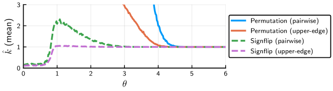
| (pairwise) | ||||
| (upper-edge) |
Parallel analysis (PA), introduced by Horn (1965), and its permutation version (Buja and Eyuboglu, 1992) are among the most popular methods for rank selection. The key idea is that we expect components rising above the noise to produce data singular values rising above their “null” pure-noise analogues. Generating “parallel” datasets, e.g., via column-wise permutation, gives estimates of these null singular values, providing data-driven cut-offs. More broadly, PA is related to invariance-based randomization tests, see e.g., (Lehmann and Romano, 2005, Chapter 15), Dobriban (2021).
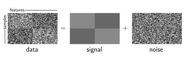
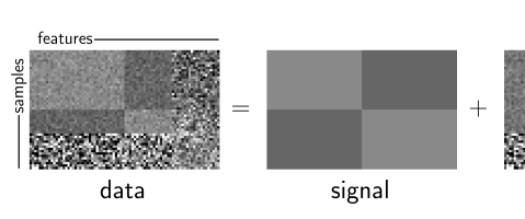
The permutation version, which we call Permutation PA, is described in Algorithm 1 and we illustrate it for a rank-one example in Fig. 1. First we form the data matrix ( data points and features). In our example this is a rank-one signal in homogeneous noise as shown in Fig. 1(a). Then we shuffle each column of independently by randomly permuting its entries, forming permuted data as shown in Fig. 1(b). Each column has a random permutation independent from all other columns. Repeating this times and collecting the singular values from each trial, we form an empirical (marginal) distribution for each singular value of , as shown in Fig. 1(c). The procedure concludes by selecting the number of leading data singular values that rise above a chosen percentile (e.g., , or ) of their permuted analogues. In our example this correctly selects one component. This is a pairwise and sequential criterion, shown in Algorithm 1 as pairwise. We start from the first data singular value, including it if it is larger than the percentile of the first permuted-data singular value, and moving on to the second singular values, and so on. We stop the first time this criterion fails.
While this pairwise comparison is the classical method, another popular alternative in practice is to compare all data singular values against the percentile of only the first permuted singular value. Indeed, some recent methods even aim to directly estimate the noise upper-edge (Dobriban and Owen, 2018). We will distinguish this method by calling it upper-edge comparison since it compares against the largest (or upper-edge) of the permuted singular values. Algorithm 1 shows this option as upper-edge. This method has the benefit of only requiring the calculation and storage of the first singular value, i.e., the operator norm , of the permuted data. Moreover, it provides a more conservative threshold and less frequently over-selects, as we see in the numerical experiments of Sections 6.1 and 6.2.
In Fig. 1(b), observe that the rank-one block structure visible in the original data becomes lost in the permuted data. This instead looks noise-like, and Permutation PA correctly selects one factor. Though this example is intentionally simple to focus on illustrating the procedure, the same occurs in general. Permutation PA is incredibly effective in practice, with numerous endorsements and increasing popularity among applied statisticians, especially in the biological sciences (e.g., Brown, 2014; Lin et al., 2016). Furthermore, it is a natural method that can be intuitively understood without appealing to sophisticated theoretical tools. Taken together with its simplicity (only a few lines of code!), Permutation PA is an incredibly attractive method in practice as well as a great foundational tool to study and build upon.
Buja and Eyuboglu (1992) provided some basic theoretical justification from the perspective of hypothesis testing, working under a certain null distribution. Assuming independent and identically distributed (i.i.d.) data points, i.e., rows, the permutation distribution of the matrix is the conditional null distribution under a non-parametric null of complete independence, conditioning on the minimal sufficient statistic under . The minimal sufficient statistic is the -tuple of empirical distributions of each column. Viewed through this lens, Permutation PA is a sort of quasi-inferential method. A theoretical justification under large-dimensional signal-plus-noise models was developed in recent years by Dobriban (2020). Using tools from random matrix theory, this work rigorously analyzed how permutations destroy signal structure while preserving the noise, providing a precise explanation as well as sufficient conditions for consistent selection by Permutation PA of so-called “above-noise” factors.
Building on the insights from Dobriban (2020), Dobriban and Owen (2018) proposed a deterministic variant. Continuing theoretical insights into the application of parallel analysis ideas for modern large-dimensional settings is an exciting and burgeoning research front; see, e.g., Zhou (2019); McKennan (2020); Chen and Li (2020); Fan et al. (2020). In this paper, we take a step towards further developing and using these insights to improve robustness to the heterogeneity we expect to become an increasingly common part of modern data analysis.
2.2 Data with heterogeneous noise and the need for new techniques
Heterogeneous noise arises very naturally in modern settings, whether due to heteroskedasticity in the features or due to heterogeneous quality among data points. For example, the noise level in medical imaging varies both within images and from image to image. Likewise, atmospheric corruptions in astronomical data vary both from night to night and from pixel to pixel, and the quality of environmental sensors can vary from location to location. These types of effects all contribute to heterogeneity in the noise. Moreover, we expect such heterogeneity to only become more common, especially as datasets are increasingly built up from data points collected at myriad and varying places, times or by varying equipment.
Consequently, recent works have begun to study how to properly account for heterogeneous noise when carrying out PCA for large data. Much work centers on improving the quality of the estimated components by, e.g., correcting for bias due to heterogeneity across features (Zhang et al., 2018), or by using an optimal spectral shrinkage after whitening the noise (Leeb and Romanov, 2018). Other methods include optimal denoising with respect to losses that account for heterogeneity (Leeb, 2019), or optimal weighting of data points to account for heterogeneity across data points (Hong et al., 2016, 2018a, 2018b). While much work remains, indeed great progress has already been made. However, fewer works have addressed the question of how to estimate the number of components in these heterogeneous settings.
For heterogeneity across features, Leeb and Romanov (2018) consider selecting the singular values rising (at least slightly) above the asymptotic operator norm of the noise matrix. This can be predicted when the noise is whitened or when the noise variances are well-estimated. Ke et al. (2020) consider a setting where these noise variances are drawn from a Gamma distribution, and propose exploiting this knowledge by first fitting the Gamma distribution from the bulk singular values. The problem of rank selection without exact or distributional knowledge of the variances, when noise is heterogeneous across both features and data points, has remained relatively open and is the setting of our work.
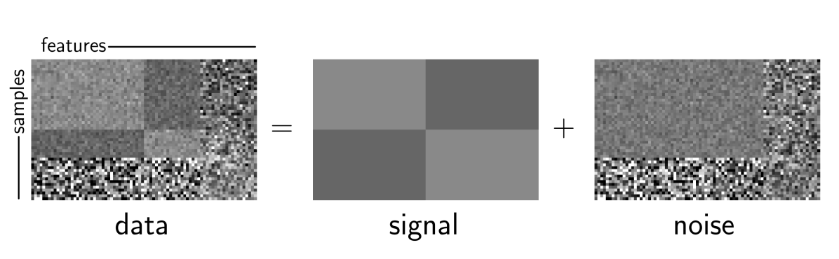
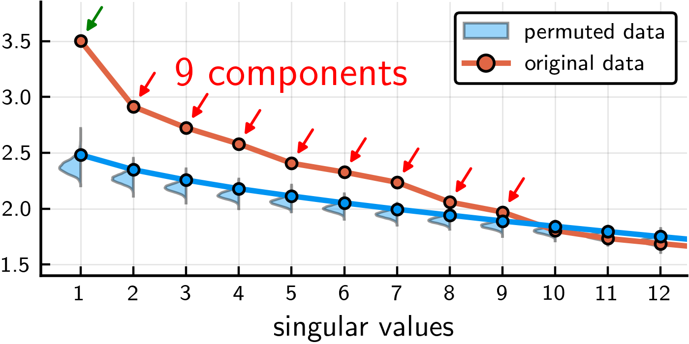
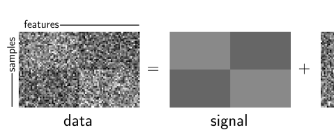
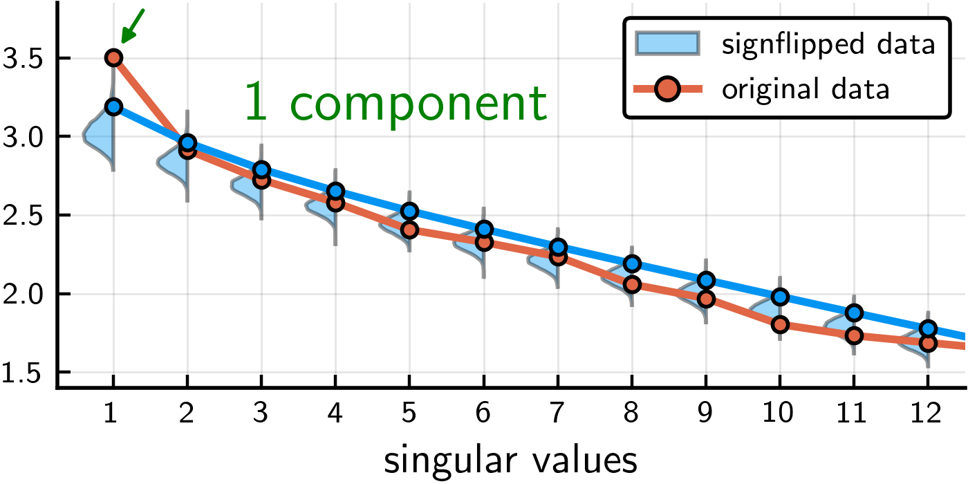
One might hope to use existing approaches, such as Permutation PA, that are rigorously grounded and battle-tested in the homogeneous setting. However, it turns out that Permutation PA can severely underperform in these heterogeneous settings. We illustrate this in Fig. 2 for a simple rank-one signal in heterogeneous noise. In this example, the noise variance varies throughout the data. The data matrix is moderately noisy on the right side, least noisy in the upper left, and most noise in the lower left. Permutation PA is not effective here. It incorrectly selects nine factors, over-selecting by eight. Moreover, this loss in performance is not unique to Fig. 2, and can happen in general when the noise is heterogeneous. Roughly speaking, permutations “smear” and homogenize the noise in a way we will make precise in Section 4.5, where we also provide a detailed explanation and characterization of this phenomenon.
Summarizing, while Permutation PA is incredibly effective and enjoys many theoretical guarantees in the homogeneous setting, it is far less so in the increasingly important case where noise is heterogeneous. New methods and theory are needed.
3 Proposed method: Signflip parallel analysis
| (pairwise) | ||||
| (upper-edge) |
The dramatic degradation of Permutation PA under heterogeneous noise could naturally lead one to consider abandoning the approach in this setting. However, we propose an elegant and simple modification that largely retains the excellent performance of parallel analysis under homogeneous noise, while expanding these benefits to data with heterogeneous noise.
Specifically, we propose replacing random permutations with random entrywise signflips. We call the resulting method Signflip PA. For clarity, we describe the full procedure in Algorithm 2, but note that it is essentially the same as Permutation PA (Algorithm 1) except for Algorithm 2. Now we generate signflipped data , where denotes the Hadamard (entrywise) product, and has i.i.d. Rademacher entries, i.e., each entry is or with equal probability. Put another way, we flip the sign of each entry with probability one-half, independent of the rest.
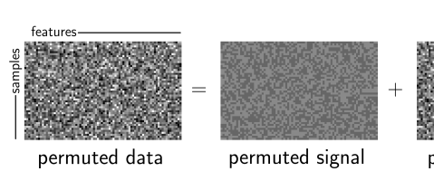
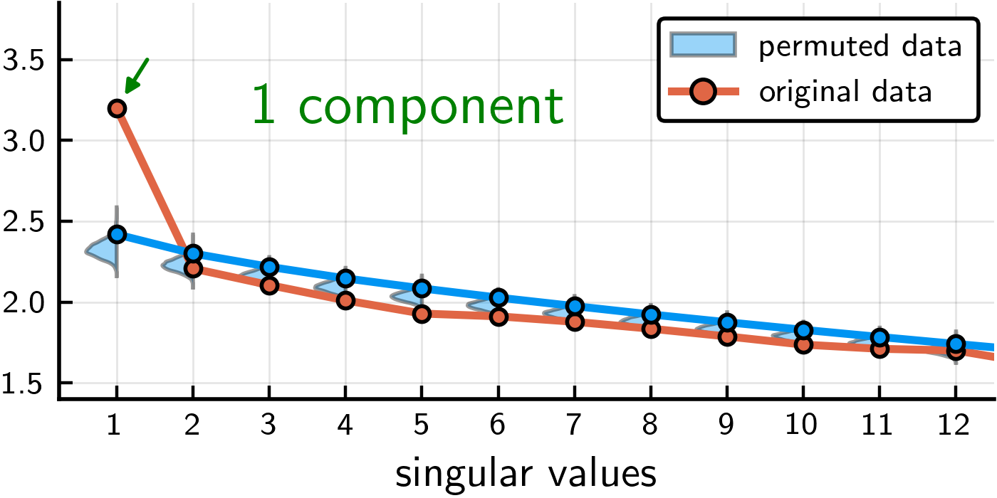
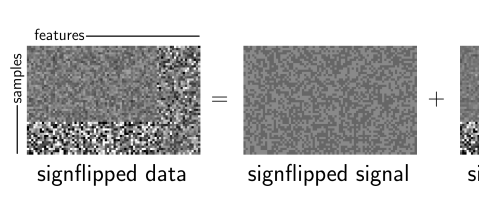
Fig. 3 illustrates the process for the same heterogeneous data as Fig. 2, for which Permutation PA incorrectly selected nine components. As shown in Fig. 3(a), we begin by independently signflipping each entry of the data matrix , forming signflipped data . Observe how the rank-one signal that can be visually seen in the data is no longer visible after signflipping, while the heterogeneous noise profile remains. The remainder proceeds analogously to Permutation PA. We repeat times and collect the singular values from each trial, forming an empirical (marginal) distribution for each singular value of , as shown in Fig. 3(b). Finally, we select the number of leading data singular values that rise above the percentile of their signflipped analogues in the pairwise and sequential way stated in Algorithm 2 as pairwise. Signflip PA correctly selects one component.
As before, we also consider the popular method of upper-edge comparison upper-edge that compares all data singular values against (the percentile of) only the first signflipped singular value. Which selection rule to choose tends to depend on the application and the salient priorities. Recall that upper-edge comparison never selects more factors than pairwise comparison, making it more conservative (see examples in Sections 6.1 and 6.2). Moreover, upper-edge comparison has the benefit of only requiring us to calculate and store the first singular value, i.e., the operator norm , of the signflipped data. The two selection rules turn out to be essentially asymptotically equivalent as for fixed , and in many settings they agree. Indeed, with either selection rule, Signflip PA correctly selects one component in this example.
The simplicity of just replacing permutations with signflips is one of the standout features of Signflip PA, as it immediately inherits many of the same practical benefits enjoyed by Permutation PA. It is an equally natural method that can be easily digested and understood without appealing to sophisticated theoretical results. It is also easy to implement, again taking only a few lines of code. These features highlight the benefit of building on the framework of parallel analysis. A thorough characterization of its performance does indeed require nontrivial theoretical work; our analysis in Section 4 leverages recent breakthroughs in random matrix theory. However, even the overall ability of signflips to preserve heterogeneous noise may be believable at an intuitive level given that each noise entry is treated separately.
Signflip PA also admits a natural interpretation as a sort of quasi-inferential method when viewed through the lens of independence testing. Assume independent but not identically distributed rows. Let be the null that the columns are independent and the marginal entry distributions are all symmetric about zero. Then, the minimal sufficient statistic becomes the array of absolute values and the signflip distribution is the conditional null distribution. See also Bordenave et al. (2020) for different uses of sign-flips in sparse matrix completion. Section 4 analyzes Signflip PA under signal-plus-noise models by extending the framework developed in Dobriban (2020). We show that Signflip PA is able to “destroy” low-rank signals in very general settings by estimating the noise level. The main implication for factor models is given in Theorem 5.3.
4 Theoretical analysis and guarantees
This section gives theoretical insight to answer the important question: how does Signflip PA work, and when does it work in general? Building on the framework developed in Dobriban (2020), we analyze general signal-plus-noise models and characterize when signflipping: a) “destroys” low-rank signal structure, and b) “recovers” heterogeneous noise.
We will make all these notions precise below, but the overall intuitive picture is shown in Fig. 4. The underlying low-rank signal structure is scrambled by signflipping (producing a matrix with much smaller operator norm), while the signflipped noise is essentially indistinguishable from the original noise (and has very similar singular values). As a result, the signflipped data looks like the noise (including its heterogeneous variance profile), and in particular has very similar singular values. Our theoretical analysis makes these rough observations rigorous.
After some background and notational clarifications (Section 4.1), we begin by characterizing signal destruction by signflips (Section 4.2), followed by an analysis of corresponding noise level estimation (Section 4.3). Finally, we explain why signflips are uniquely suited (Section 4.4) and in what way permutations homogenize heterogeneous noise (Section 4.5). Carefully leveraging recent breakthroughs in random matrix theory enable us to obtain elegant and simple conditions throughout.
4.1 Notations and preliminaries
To make the following discussions precise, we detail our notations and provide some relevant theoretical background here.
Notations. Throughout the paper, we denote the Hadamard product (entrywise multiplication) of two matrices and of the same size by . For an matrix , we use and to denote the spectral norm and the Frobenius norm, respectively. Let be the matrix whose -th entry is the absolute value of the -th entry of . Let denote the matrix norms induced by vector norms, and denote the entrywise matrix norms. They are defined as follows
where denote the -norm for vectors. The norm will play a special role; it is the maximum of the norms of the columns of . Similarly, is the max of the norms of the rows of .
We denote the trace of a matrix by . For two random matrices , means that the matrices have the same distribution, thus implying that the corresponding -entries of and have the same distribution. We use the classical big-O and little-o notations to describe the asymptotic relationship between two quantities. We call a random variable a Rademacher random variable if . We use to denote that for a universal constant which does not depend on any parameter of the problem unless stated explicitly. We will use if and .
Statistical model. The model we will consider in this paper is the following. The data matrix has data points and features. The rows of are independent -dimensional observations, not necessarily identically distributed. We can express in the following “signal-plus-noise” form:
Here is the “signal” part, which is typically of low rank. We denote the unknown rank; this is the key parameter we aim to estimate. The “noise” part is modelled as , where has i.i.d. random entries with zero mean, unit variance, and finite fourth moment, is a deterministic matrix with -entry . Thus, has independent entries and the -entry has variance . We say that has a general variance profile, where the profile matrix is . This model is a generalization of the standard factor model. In the standard factor model, within each column of , all entries have the same variance.
Define the aspect ratio of as . We will work in the proportional limit regime (e.g., Marchenko and Pastur, 1967; Serdobolskii, 2007; Johnstone, 2007; Yao et al., 2015, etc), where we consider a sequence of problems with growing parameters such that as . For a positive semidefinite matrix , let be its eigenvalues, and its empirical spectral distribution be defined as
As usual, we will typically assume converges weakly to a limiting spectral distribution . For a non-square matrix, we can still define its empirical spectral distribution, by using its singular values instead. For a bounded probability distribution , we define its upper edge to be
Random matrix theory. Now, we will briefly talk about some needed results from random matrix theory (RMT). See Bai and Silverstein (2010); Couillet et al. (2011); Yao et al. (2015) for references. We assume the design matrix is generated as for an matrix with i.i.d. entries, satisfying , , and . The empirical spectral distribution of the positive semidefinite matrix has a limiting spectral distribution, in the sense of weak convergence. Under these assumptions, a central result in this area is the Marchenko-Pastur theorem (Marchenko and Pastur, 1967; Bai and Silverstein, 2010), which says that the empirical spectral distribution of the sample covariance matrix converges weakly to a limiting spectral distribution almost surely as . Moreover, the largest eigenvalue of will also converge almost surely to the upper edge of . A common approach to prove this type of result is to use the Stieltjes transform. For a probability distribution over , the Stieltjes transform of is a complex analytic function defined as
An important property of the Stieltjes transform that uniquely determines . The intuition behind this approach is that for a symmetric matrix , the Stieltjes transform of its empirical spectral distribution is
Thus, in order to study the convergence of the empirical spectral distribution , we can work with the Stieltjes transform instead, which boils down to work with the resolvent matrix . For , there are many matrix inversion lemmas and matrix identities we can use. Similar results based on singular values also hold for non-square matrices.
4.2 Signal destruction by signflips
Here we describe our results on signal destruction by Signflip PA, needed for the general theory of consistent signal selection. One might wonder in what sense signflipping “destroys” the signal, given that there is no reduction in Frobenius norm, i.e., . In other words, the sum-of-squares of the singular values are unchanged. The key is that signflipping takes low-rank signals (for which this sum is dominated by the first few singular values) and makes them “noise-like” (with the energy spread out among all singular values). Consequently, the signal is destroyed in operator norm: .
This section proves sufficient as well as necessary conditions for signals guaranteeing that as , either in or almost surely. Recall that convergence and almost sure convergence both imply convergence in probability. We provide conditions for general signal matrices as well as sums of outer products (which are common in many applications). We finally show that our conditions are in fact optimal for signals with uniformly bounded rank. The conditions we find for Signflip PA are generally simpler and sharper than those found for Permutation PA (Dobriban, 2020), even for homogeneous noise. This is because we are able to build on recent breakthroughs and a deep understanding of heterogeneous random matrices with independent entries.
4.2.1 General conditions guaranteeing signal destruction
We begin with our most general conditions for signal destruction, which build on an extensive line of works on the operator norm of random matrices with independent heterogeneous Gaussian entries (e.g., Latała, 2005; Bandeira and Van Handel, 2016; Latała et al., 2018, and references therein). In particular, the major breakthrough in Latała et al. (2018) characterizes the precise dimension-free behavior of the Schatten norms of these matrices. We adapt it to our setting by relating this to the operator norm of signflipped matrices, and build on it by deriving bounds in terms of the signal rank.
We need the following decay coefficient (which we referred to as the “logarithmic decay coefficient” above), measuring the rate of decay of the row and column norms:
| (1) |
Here denotes the -th largest column norm, i.e., sorts the column norms in descending order. Intuitively, if the row and column norms of decay quickly, then is small.
We will assume that the rows and columns of have asymptotically vanishing norms in expectation, which turns out to be necessary (Section 4.2.3). One can verify that if they do not vanish, then the operator norm of cannot converge to zero (consider the canonical basis vectors to get a lower bound). We allow both random and deterministic signals.
Theorem 4.1 (Asymptotic signal destruction).
Let be a sequence of signal matrices, and let be a sequence of Rademacher random matrices of corresponding size. Suppose that has asymptotically vanishing column/row norms in expectation: and . Then we have as ,
-
convergence:
if additionally either:
-
(a)
the expected operator norm of decays to zero: ,
-
(b)
the decay coefficient 1 vanishes in expectation: , or
-
(c)
the expected largest column/row norms vanish fast enough:
and .
Moreover, sufficient condition (b) is guaranteed under any of the following conditions:
-
•
the norm of the entries of vanishes: for some ,
-
•
, or
-
•
is uniformly bounded.
-
(a)
-
Almost sure convergence:
if there exists for which is summable (over ), i.e., .
When is deterministic, the expectations with respect to are dropped. This theorem (proved in Section A.2) provides general conditions under which signal destruction is guaranteed by random signflips. Recall that all these conditions are also sufficient conditions for convergence in probability. Roughly speaking, we require either a small signal (i.e., vanishing magnitude operator norm) or sufficient delocalization across rows and columns.
Remark 1.
Signals with uniformly bounded rank automatically have sufficient delocalization under the assumption of vanishing row/column norms. This provides a necessary and sufficient condition for such signals. We formalize and elaborate on this fact in Section 4.2.4.
Remark 2.
Sufficient condition (a) for convergence may appear simple, leading one to wonder if it is implied by either of the other two. However, this is not the case. Consider with . One can verify and , and indeed (in fact, this is deterministically true). However,
Hence we see that sufficient condition (a) is not redundant. It captures signals that do not delocalize per se and essentially vanish on their own.
Remark 3.
For clarity and convenience, we state most of our results in the large matrix limit as , as this setting is our primary focus. However, one can verify that many of our results, especially in Theorem 4.1, generalize immediately to arbitrary sequences of signal matrices (e.g., with only growing).
4.2.2 Conditions for sums of outer products
While Theorem 4.1 is quite powerful and general, it is also very useful to consider signals written as sums of outer products, i.e.,
as these arise very naturally in practice. Some important examples are:
-
•
The singular value decomposition (SVD) , where are singular values with corresponding orthonormal sets of left and right singular vectors and .
- •
We do not require these terms to be orthogonal, nor even linearly independent. We will also later allow the number of terms (which upper bounds the rank of ) to grow with , where we typically consider the setting where . To simplify the presentation, however, we start by studying a single outer product.
Theorem 4.2 (Signal destruction for an outer product).
Let be a sequence of outer product signals with deterministic signal strength and independent signal vectors and normalized so that , and let be a sequence of Rademacher random matrices of corresponding size. Then we have as
-
convergence:
if .
-
Almost sure convergence:
if there exists for which is summable (over ).
If the signal vectors and are also deterministic, the above expectations are dropped. The theorem is proved in Section A.3.
Remark 4.
The normalization is not necessary, but simplifies some of the expressions. It also provides a natural signal representation, making it possible to reason by rough analogy to the SVD. Removing the normalization, we have convergence if .
The condition for signal destruction simplifies dramatically in this case (note that the rank is uniformly bounded), and it depends only on how fast and decay compared to the growth of the signal strength . The following corollary quantifies these rates, revealing an elegant characterization for both and almost sure convergence.
Corollary 4.3 (Conditions in terms of signal strength and delocalization rates).
Under the setting of Theorem 4.2, suppose that the signal grows at a rate of . Then as with , we have
-
convergence:
If delocalizes at rates of and , then if either: a) , or b) and .
-
Almost sure convergence:
If delocalizes so that for all , and , then if is deterministic and .
The corollary is proved in Section A.4.
Remark 5.
This parameterization is convenient because it covers many important settings. For example, when the singular vectors and are independent random vectors uniformly distributed on the unit sphere, it follows that . One can verify this fact from, e.g., Vershynin (2018, Exercise 2.5.10 and Theorem 3.4.6).
Fig. 5 illustrates the convergence regions as a function of the delocalization exponents and given signal growth exponents and . These exponents are constrained as shown by the feasible region in Fig. 5 due to the following simple bounds:
Thus, the feasible range is unless for which is feasible, or for which is feasible.
If the signal strength decays, i.e., , all feasible delocalization exponents result in signal destruction (both in and almost surely) as one might expect. This can be quickly verified by observing that the convergence region completely covers the feasible region in Fig. 5. On the other hand, if the signal grows too rapidly, i.e., , there is no overlap and none of the feasible delocalization exponents satisfy our conditions for signal destruction. Indeed, it turns out that the signal is not destroyed in this case (see Section 4.2.3 for discussion of necessary conditions). For and generated independently uniformly on the unit sphere, signal destruction in occurs as long as or with .
We now generalize Theorem 4.2 to sums of outer products, where the number of terms may grow in . The proof is given in Section A.5.
Theorem 4.4 (Signal destruction for a sum of outer products).
Let be a sequence of signals, each a sum of outer products with deterministic signal strengths and left vectors independent from right vectors , all normalized so that . Let be a sequence of Rademacher random matrices of corresponding size. Then we have
-
convergence:
if .
-
Almost sure convergence:
if there exists for which is summable.
If the signal vectors and are deterministic, the above expectations are dropped. Without normalization, a sufficient condition for convergence is . As before, signal destruction roughly occurs when the signal vectors delocalize at a rate outpacing the overall growth of the signal strength. As before, we quantify these rates, where we now additionally suppose the number of terms grows as , where we call and the rank growth exponents. The rank of may be lower than due to the potential for linear dependence among the terms. The following corollary shows how rank can grow in this more general setting; the proof is given in Section A.6.
Corollary 4.5 (Conditions in terms of signal rank, strength, and delocalization rates).
Under the setting of Theorem 4.4, suppose the signal has rank growing as and signal strength growing as . Also suppose the signal norms are deterministically bounded as
Then as with , we have
-
convergence:
if we have: a) , or b) and .
-
Almost sure convergence:
if is deterministic and .
The rank effectively inflates the signal strength since signflips must now destroy all terms in the sum, which requires a greater amount of delocalization. This produces a trade-off between the signal growth and the rank growth; they cannot both grow rapidly. In many applications , i.e., the rank of the signal is uniformly bounded. This is a common setting in factor analysis and PCA. In this case, the conditions essentially reduce to the rank-one case. However, our theory allows for much more general settings.
4.2.3 Necessary conditions
This section establishes some properties the signal must have to be destroyed by random signflips. We start with the following observation.
Lemma 4.6 (Sign-invariant operator norm bounds).
Let be a sign-invariant lower bound on the operator norm (up to a constant), i.e., and . If for Rademacher random matrices , then .
The lemma follows immediately from
Combined with standard inequalities for matrix norms, it leads to the following concrete necessary conditions for signal destruction (whose proof is omitted).
Theorem 4.7 (Necessary conditions for asymptotic signal destruction).
Let be a sequence of signal matrices, and let be corresponding Rademacher random matrices. We can have only if the column/row norms vanish in : and . Likewise, only if the following expected matrix norms vanish:
As with the sufficient conditions before, we also provide necessary conditions for sums of outer products, specifically for deterministic signals in SVD form. The proof is in Section A.7. One might hope that favorable cancellation among terms might help with signal destruction. We find that this is not the case for the SVD. Essentially, each term must undergo signal destruction.
Corollary 4.8 (Necessary conditions for destruction of an SVD).
Let be a sequence of deterministic signals in SVD form with rank , singular values , left vectors , and right vectors . Let be corresponding Rademacher random matrices. Then requires
4.2.4 An optimal condition for bounded rank signals
Determining whether the sufficient conditions are also necessary is a hard question in general. However, for the important setting of signals with uniformly bounded rank (common for low-rank models), we discover a remarkably simple condition for signal destruction (in ) that is both necessary and sufficient. It is a direct consequence of Theorem 4.1 and Theorem 4.7.
Theorem 4.9 (Necessary and sufficient condition for signals with uniformly bounded rank).
Let be a sequence of signals with uniformly bounded rank, i.e., , and let be the corresponding Rademacher random matrices. Then if and only if the column/row norms vanish in : and .
In particular, we find a complete characterization for the expected operator norm of signflipped bounded rank signals, namely:
Characterizing the expected operator norm of heterogeneous Rademacher random matrices beyond bounded rank heterogeneity remains an open problem.
4.3 Noise level estimation by signflips
Having analyzed when signflips destroy low-rank signals in operator norm, we now turn to the estimation of the noise level by signflips. We briefly discuss the case covered by Permutation PA, which Dobriban (2020) studied by considering the strong condition of noise invariance. Namely, , where the equality in distribution is taken with respect to both the noise and independent column-wise permutations . In that case, one can allow noise of the form
Here is an matrix of i.i.d. standard Gaussians, is diagonal, , and is a PSD matrix. The term adds a per-column-fixed random variable to each entry. This is allowed by the theory, but it is rarely of practical interest. Thus, we will consider noise models of the form . We also need the convergence of the operator norm: as , which is guaranteed by Proposition 4.2 of Dobriban (2020). Essentially, Permutation PA works well when the noise is homogenous in the sense that different rows (data points) have the same variance within each column (feature). This is the standard model used in factor analysis.
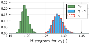
Signflip PA also works for this model. Gaussian random variables are symmetric, i.e., , so it follows that for any fixed signflip matrix , and likewise for random (independent of ). However, Signflip PA also works beyond this noise model. Suppose the noise matrix has independent normal entries with heterogeneous variances. Then we say has a general variance profile. Clearly, we still have so signflips continue to be effective.
How about relaxing the Gaussianity assumption on the noise entries? For Permutation PA, this is not a problem because still holds even when the entries of noise are not Gaussian random variables. But for Signflip PA, when the noise entries are not symmetric random variables, we do not have in general. This may appear to be an issue for Signflip PA at the first glance. However, due to the well-known universality phenomenon in random matrix theory (e.g., Tao and Vu, 2011; Erdős et al., 2011), it turns out that Signflip PA can also work beyond Gaussian entries. The key idea is that sign invariance can be replaced with a weaker notion of noise level estimation that is sufficient for our purposes. We explain this below. We begin with the following definition.
Definition 4.10.
We say that a random variable has a sharp sub-Gaussian Laplace transform (Guionnet and Husson, 2020) if
We will sometimes say (as shorthand) that is a sharp sub-Gaussian random variable.
Remark 6.
The term “sharp” comes from the observation that if a random variable is sub-Gaussian for some constant ,
then and =Var. Some simple examples are of sharp sub-Gaussian random variables are centered Gaussian random variables, Rademacher random variables, and uniform random variables on . We can generate more complex examples using that for any , has a sharp sub-Gaussian Laplace transform when are independent sharp sub-Gaussian random variables. One can refer to Guionnet and Husson (2020) for more details.
Then, we have the following theorem, based on results from Girko (2001); Couillet and Debbah (2011); Husson (2020). We apply it to show that for noise with a general variance profile, there is a limiting spectral distribution. Moreover, the largest singular value of converges to the supremum of the support of the limiting spectral distribution. Thus, Signflip PA can preserve the limiting spectral distribution as well as the limit of the largest singular value. This result is essential, since it provides a rigorous justification for Signflip PA under heterogenous noise models.
Theorem 4.11 (Sign-invariant heterogenous noise models).
Let , where has independent sharp sub-Gaussian entries with zero mean and unit variance, and is a variance profile satisfying one of the following conditions111 has variance :
-
Piecewise constant variance profile:
Let and be two partitions of such that and , where are fixed. Denote the piecewise constant function defined by if and , where and . Then, consider defined by .
-
Continuous variance profile:
Let be a continuous function. Suppose satisfies
Then the noise is sign-invariant, i.e., as with for any (fixed with respect to ) where is the corresponding Rademacher random matrix.
In particular, the empirical spectral distributions of and both converge weakly to a deterministic distribution with probability one, and for any fixed , where is the rightmost point in the support of .
The proof is given in Section B.1. In conclusion, the largest singular value of the true noise and the signflipped noise have the same limiting value. This shows that Signflip PA asymptotically estimates the proper noise level, which is the limit of the top true noise singular value. This implies that it uses the correct threshold for selecting factors, and it can thus consistently estimate the number of above-noise factors. We will state this precisely later.
4.4 Uniqueness of signflips
The form of Signflip PA suggests a natural generalization: use as the “null” data, where has i.i.d. entries with zero mean and unit variance that are not Rademacher random variables. For example, one might consider using a matrix with i.i.d. standard normal entries. This raises the question, is there something special about signflips or can anything be used? Might there be a better choice?
From a pragmatic perspective, it is perhaps enough to know that signflips are effective. Especially so, given that signflips have the added practical benefit of being efficient to generate and easy to use. Nevertheless, the prospect of a better or even optimal choice is alluring and is moreover an interesting theoretical question. However, it turns out that signflips are in some sense uniquely suited for deriving theoretical guarantees, as we now describe.
A key step in proving noise recovery for heterogeneous noise in Theorem 4.11 was proving convergence of the operator norm of to the upper-edge of its limiting spectral distribution. We accomplished this by establishing that each of the entries of has a sharp sub-Gaussian Laplace transform. This condition is important, and one can refer to the recent works Guionnet and Husson (2020); Husson (2020) for more details. It is not hard to see that does not satisfy this assumption in general. For example, suppose both were Gaussian, i.e., and . Then is the product of two independent standard Gaussians and is no longer sub-Gaussian, let alone sharp sub-Gaussian. In fact, the following proposition shows that Rademacher random variables are the only choice for for which has sharp sub-Gaussian Laplace transform when is Gaussian.
Proposition 4.12 (Sharp sub-Gaussianity implies signflips for Gaussian noise).
Let be a standard normal random variable and be a random variable with zero mean and unit variance which is independent of . If has a sharp sub-Gaussian Laplace transform, then must be a Rademacher random variable.
The proof is given in Section B.2. Thus, signflips are uniquely suited for establishing convergence under general noise distributions, at least based on our current theoretical tools. This does not imply that other distributions will necessarily perform poorly, and the opportunity to find better choices remains, e.g., one might try to tailor the choice given certain noise properties. Simply put, other choices fall outside the bounds of our current analysis techniques and would require new approaches to derive guarantees.
4.5 Noise homogenization by permutation
This section explains why Permutation PA degrades for heterogeneous noise. Consider noise as in Theorem 4.11, i.e., are independent with variance . Let denote the array of independent random permutations used by Permutation PA ( permutes the entries of the th column). Then one can verify that the marginal variance of is , where the variance is taken with respect to both and . Namely, is a homogenized version of obtained by averaging variances within each column. The permuted noise has a homogenized (marginal) variance profile , so we might expect the spectrum of permuted noise to behave more like a noise matrix with profile than the actual profile .
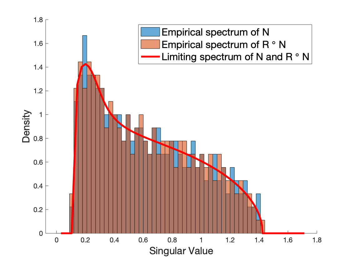
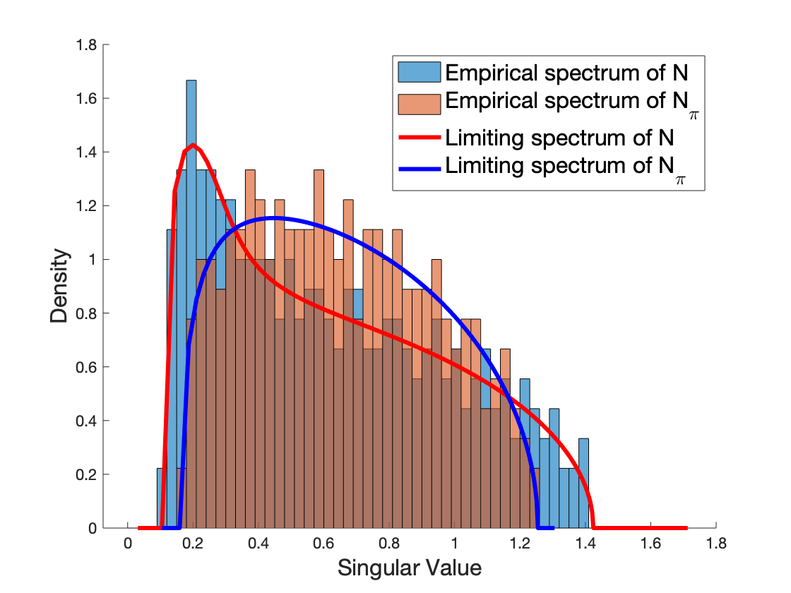
Indeed, this intuition plays out in practice, which we illustrate with a simple example in Fig. 6. We generate an noise matrix with independent normal entries, where and . The first data points have entries with variance , while the remainder have entries with variance . This is a piecewise constant variance profile, and indeed signflipped noise accurately recovers the noise spectrum (Fig. 6(a)). On the other hand, the empirical spectral distribution of permuted noise is quite different from that of the noise; permutation significantly shrank the spectrum. This is the general reason Permutation PA suffers under heterogeneous noise. Permutations homogenize the noise, leading to unreliable estimates of the noise level, and consequently an inaccurate selection of the number of factors.
Using SPECTRODE (Dobriban, 2015) we compute and overlay the limiting spectral distributions for random matrices with independent entries and variance profiles and . Note that here, and for all . The spectrum of closely matches the limiting spectral distribution for the profile , even though does not actually have independent entries (due to the permutation). This naturally leads one to conjecture that the limiting spectral distribution of is nevertheless the same as that for a matrix with independent entries and variance profile . This conjecture is in fact true, as we state in the following theorem that concludes the theoretical explanation by providing a rigorous characterization of the limiting spectrum of permuted noise under heterogeneous variance profiles.
Theorem 4.13 (Permutations homogenize variance profiles).
Let , where is a sequence of deterministic variance profiles and has independent entries with zero mean, unit variance, and uniformly bounded fourth moments. Suppose has nonnegative uniformly bounded entries and its column mean squares,
have empirical distribution converging to a deterministic distribution . Then as with , with probability one, the empirical spectral distribution of for permuted noise converges weakly to the generalized Marchenko-Pastur distribution, whose Stieltjes transform satisfies:
| (2) |
A key special case is when , i.e., all column mean squares of are unity. In this case, has a spectrum like a random matrix with i.i.d. entries.
To prove Theorem 4.13, we first prove the following lemma. It establishes a generalized Marchenko-Pastur law under relaxed independence conditions, and is of independent interest. We allow dependence among entries while imposing conditions on the population covariances of the rows. For some other related (but different) results, see Hui and Pan (2010); Wei et al. (2016); Bryson et al. (2019). For a complex-valued random variable , we define .
Lemma 4.14 (Generalized Marchenko-Pastur with relaxed independence conditions).
Let be a sequence of zero mean random matrices with independent rows. Suppose that with and furthermore:
-
1.
Each row of has isotropic covariance matrix .
-
2.
The variances are uniformly bounded with empirical distribution converging to some deterministic distribution .
-
3.
For any sequence of possibly complex-valued symmetric deterministic matrices with uniformly bounded spectral norms, and for every row , we have
(3) where does not depend on the sequence .
Then, with probability one, the empirical spectral distribution of converges weakly to the generalized Marchenko-Pastur distribution, whose Stieltjes transform satisfies:
| (4) |
This lemma is proved in Section B.3 by carefully combining techniques used in the proofs of (Bai and Zhou, 2008, Theorem 1.1) and (Bai and Silverstein, 2010, Theorem 4.3). With this lemma in hand, we prove Theorem 4.13 in Section B.4. The key is to show the permuted noise matrix satisfies all the conditions of Lemma 4.14, of which especially crucial is the concentration of quadratic forms 3.
5 Implications for rank selection
This section explains the implications of the general theoretical characterization for rank selection. In particular, we will prove that Signflip PA is asymptotically accurate, in a sense which we now precisely define.
Definition 5.1 (Asymptotically perceptible factors and accurate selection).
Suppose is a sequence of data matrices for which the noise upper-edge converges in probability: . Then, as , we say the -th factor is
-
perceptible (in probability)
if for some .
-
imperceptible (in probability)
if for some .
In particular, if in probability, then it is perceptible if and imperceptible if . We say a selection is perceptive if it includes all perceptible factors and no imperceptible factors.
This notion was introduced in Dobriban (2020) and naturally captures which factors are asymptotically meaningful and “rise above the noise”. Factors falling “below the phase transition” asymptotically tend to produce essentially noise-like factors (see, e.g., Baik et al., 2005; Baik and Silverstein, 2006; Benaych-Georges and Nadakuditi, 2012; Dobriban and Owen, 2018; Dobriban, 2020). While the signal rank may grow in , the number of perceptible factors is an asymptotic property of the sequence. Convergence of the noise upper-edge to a noise level , ensures that our setting has a meaningful asymptotic notion of the noise “level” or “floor”. In this setting, we can hope to consistently estimate factors rising above the noise.
We now to bridge this notion with the theoretical characterization of signflips. Related (but slightly different) lemmas appear in Dobriban and Owen (2018); Dobriban (2020).
Lemma 5.2 (Consistency).
Suppose that data has both
-
•
Signal destruction: in probability, and
-
•
Sign-invariant noise: for any fixed , in probability,
where is the corresponding Rademacher random matrix. Then signflips consistently recover each noise singular value, i.e., for any fixed , in probability. Additionally, Signflip PA with upper-edge comparison is perceptive (i.e., selects all perceptible factors and no imperceptible ones) with probability tending to one, if the noise upper-edge converges, i.e., in probability. Finally, signflip PA with pairwise comparison is also perceptive with probability tending to one if each leading noise singular value similarly converges, i.e., for any fixed , in probability.
The proof is given in Section C.1.
Remark 7.
Both perceptibility (Definition 5.1) and consistency (Lemma 5.2) are in probability for convenience in this section, but one can verify that the analogous notion and statement also apply for almost sure convergence.
Remark 8.
One may wonder why signal destruction is crucial. Roughly speaking, the main adverse effect is a general inflation of the noise singular values which can lead to under-selection as perceptible factors fall below the inflated threshold. This is called shadowing, see e.g., Peres-Neto et al. (2005); Dobriban (2020) and references therein.
We illustrate the power of our theoretical characterization for the important setting of factor analysis. In particular, consider the standard linear common-factor model (e.g., Anderson, 2003; Brown, 2014; Dobriban, 2020). Under this model, the data matrix can be written as
where is the fixed factor loading matrix, is an random matrix containing the factor values, and is the idiosyncratic noise matrix. In the standard setting, has i.i.d. rows with covariance matrix
Here is the diagonal matrix of idiosyncratic variances and Cov is the covariance matrix of the factor values.
Our main result is that Signflip PA can correctly select the perceptible factors in a more general factor model, where the noise can have a general variance profile. As discussed above, permutation PA will fail in this setting. Before we state our result, it is convenient to define the scaled factor loading matrix .
Theorem 5.3 (Main result: Signflip PA selects the perceptible factors in general heterogeneous noise).
Suppose we have a factor model , where we observe data points and each sample is a -dimensional vector. Assume the following conditions:
-
1.
Asymptotics. The aspect ratio as .
-
2.
Factors. The number of factors can grow with . The rows of the matrix are the factor values of the data points. The -th row has the form , where has independent sub-Gaussian entries with zero mean and unit variance.
-
3.
Idiosyncratic noises. The noise has a general variance profile, where and are as in Theorem 4.11.
-
4.
Factor loadings. The scaled factor loading vectors are delocalized, in the sense that and .
Then, with probability tending to one, Signflip PA selects all perceptible factors and no imperceptible factors.
The proof is given in Section C.2.
Remark 9.
For Permutation PA with fixed number of factors and a more restricted noise setting, Dobriban (2020, Theorem 2.1) provided a sufficient condition on factor loadings of which implies and , since and . In contrast, the condition on factor loadings in Theorem 5.3 reduces to and in this case. Hence, our conditions are stronger even in the special case considered in that work.
Remark 10.
Remark 11.
Recalling that for and drawn uniformly from the unit sphere, Lemma 5.2 also immediately gives simple guarantees for rank selection in spiked models with normalized vectors and heterogeneous noise.
6 Experiments
This section demonstrates the empirical performance of Signflip PA through numerical simulations on homogeneous and heterogeneous noise, realistically generated chlorine data with heterogeneous sensor noise, and real data from single-cell RNA-sequencing.
6.1 Simulation with homogeneous noise
We start with a setting where Permutation PA excels: a rank-one signal in homogeneous noise. Specifically,
where and are unit vectors (drawn uniformly from the unit spheres in and ), and the noise has entries . We use the percentile from parallel trials, and repeat the experiment for runs.
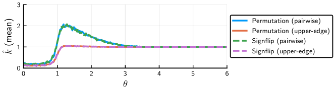
Fig. 7 shows the average rank selected by Permutation PA and Signflip PA with both selection rules, where and and we sweep across signal strengths . For small , the underlying component is imperceptible and none of these approaches select it. As grows, the methods begin to discover this component. Pairwise comparisons over-select initially due to non-asymptotic random fluctuations in the leading noise singular values. Upper-edge comparison is more conservative and mitigates the over-selection, but detects the component on average slightly later.
Notably, permutations and signflips perform similarly in this case. Since and are drawn uniformly from the sphere, they are generically delocalized and are destroyed well by both permutations and signflips. Importantly, the noise here is also homogeneous and hence preserved by both permutations and signflips. In conclusion, this experiment demonstrates that signflip PA works as well as the more well known and widely used permutation PA, even in the special case of homogeneous noise where permutation PA is applicable.
6.2 Simulation with heterogeneous noise
Now suppose of the data points have noise variance , where the remaining have noise variance as in Section 6.1. As we have discussed, such settings are quite natural in modern data analysis, e.g., when data points are collected from several instruments or sources that have varying quality. As shown in Fig. 8(a), Permutation PA now dramatically over-selects. On the other hand, Signflip PA is robust to this heterogeneity and continues to perform well.
In fact, the underlying component is discovered a bit earlier than in Fig. 7 (i.e., for smaller ) since the heterogeneous noise here is actually less noisy overall than the homogeneous noise considered there. Fig. 8(b) compares the scree plots for these two settings. The component is indeed easier to see in the heterogeneous case since the singular value gap is larger.
The effect of permutations and signflips on the leading noise singular value, as shown in Fig. 8(c), corroborate our explanation (Section 4.5) for why permutations over-select in this presumably easier setting. Permutations homogenize the noise, and as a result the leading singular value of the permuted noise is downwardly biased. Using upper-edge comparison in Permutation PA over-selects, and using pairwise comparison over-selects even more. Signflip PA, on the other hand, recovers the noise (the distribution of the leading noise singular value is essentially the same) and consequently selects the correct number of components.
6.3 Realistically generated chlorine data with heterogeneous sensor noise
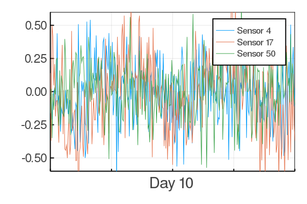
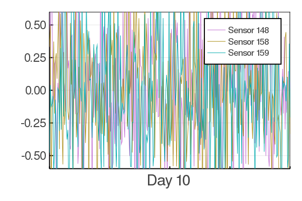
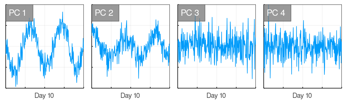
This section considers the identification of meaningful components in heterogeneous noise with underlying realistic chlorine measurements generated from EPANET for sensors at time points with a sampling period of five minutes. The data is available online222http://www.cs.cmu.edu/afs/cs/project/spirit-1/www/ and was previously studied by Papadimitriou et al. (2005); Balzano et al. (2010); as a preprocessing step, we subtract out the DC, i.e., constant, component of each time series. After an initial transient phase, the signals are roughly periodic with a period of approximately 22 hours. To simulate sensors having heterogeneous quality, as can commonly arise in practice, we add mean zero Gaussian noise with variance to the first half of the sensors (sensors 1–83) and with variance to the second half (sensors 84–166). Fig. 9(a) shows a few of the cleaner sensors for a one-day window of the data, and Fig. 9(b) shows a few of the noisier sensors for the same window.
Fig. 9(c) shows the leading four right singular vectors of the mean-centered data matrix formed from the time series as
The first two components here appear to rise above the noise and capture the underlying periodic behavior. The remaining components generally seem to have more noise than signal. Roughly speaking, they are below the noise floor and are likely to be essentially random.
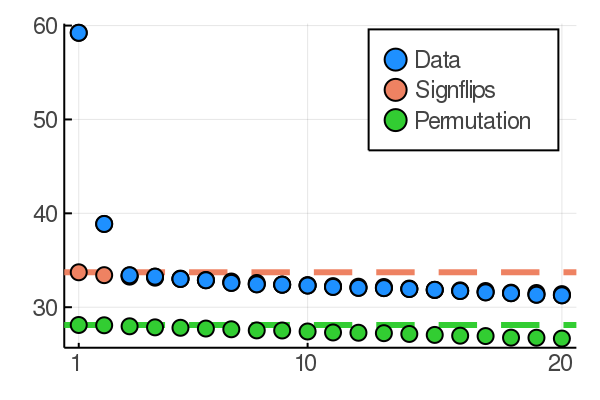
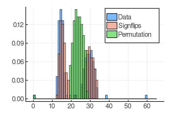
The scree plot in Fig. 9(d) shows the first 20 singular values of , along with their analogues after permutation and signflipping; a horizontal dashed line indicates the upper-edge comparison cut-off. Signflip PA selects the first two components, consistent with the observation above that these appear to have risen above the noise. Permutation PA, on the other hand, selects many more components in this example. The heterogeneous noise is homogenized by permutations, yielding a different spectrum as shown in Fig. 9(e). In contrast, signflips preserve the noise spectrum, and consequently appropriately select components that rise above the noise. Notably, signflips here even recover the approximate separation of the bulk singular values into two parts.
6.4 Single-cell RNA-sequencing data
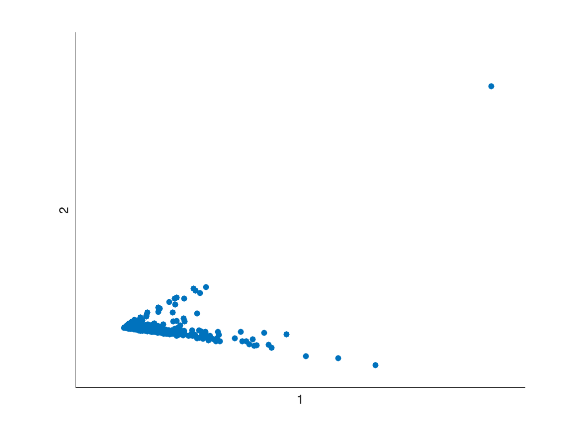
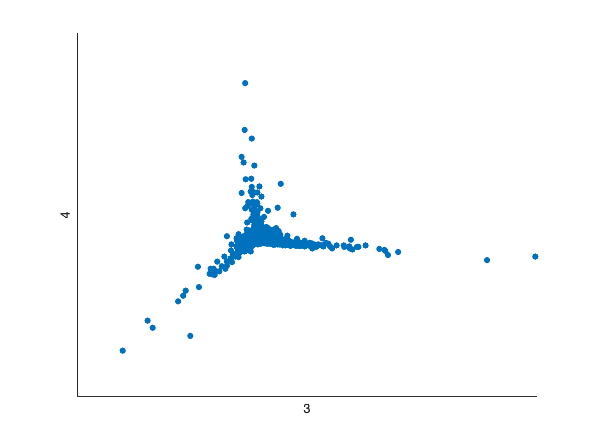
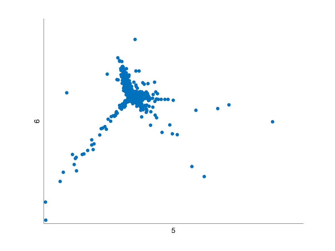
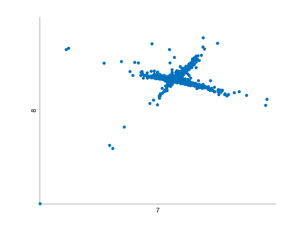
This section applies Permutation PA and Signflip PA (as well as several other popular non-PA methods) to real data from single-cell RNA-sequencing (scRNA-seq). We use the data set from Macosko et al. (2015). This new sequencing technology has been a powerful tool in the sciences for quantifying the transcriptome of individual cells (Andrews and Hemberg, 2018). The data from scRNA-seq experiments is usually high dimensional and noisy, which produces many challenges for data analysis. Moreover, heterogeneous noise may naturally arise due to heterogeneity among cells or genes. Dimensionality reduction, e.g., by PCA or t-SNE, is an important part of data processing pipelines, particularly for data visualization. It is important to determine how many principal components to keep.
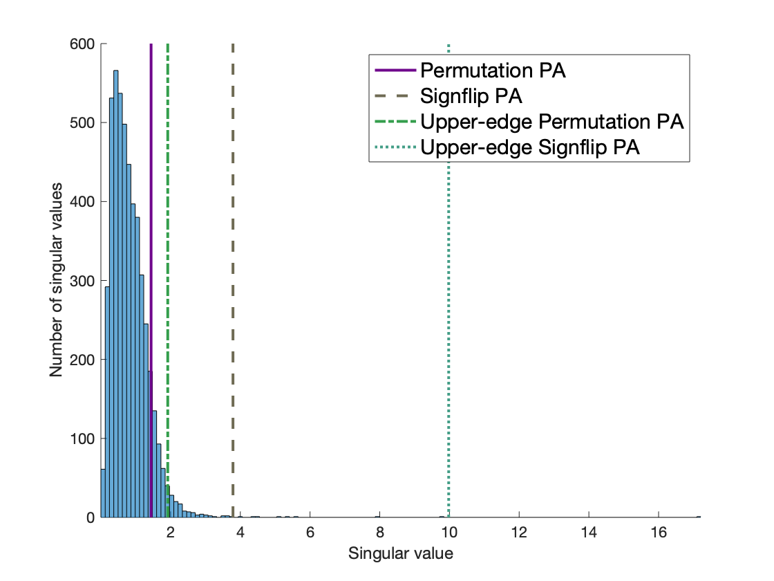
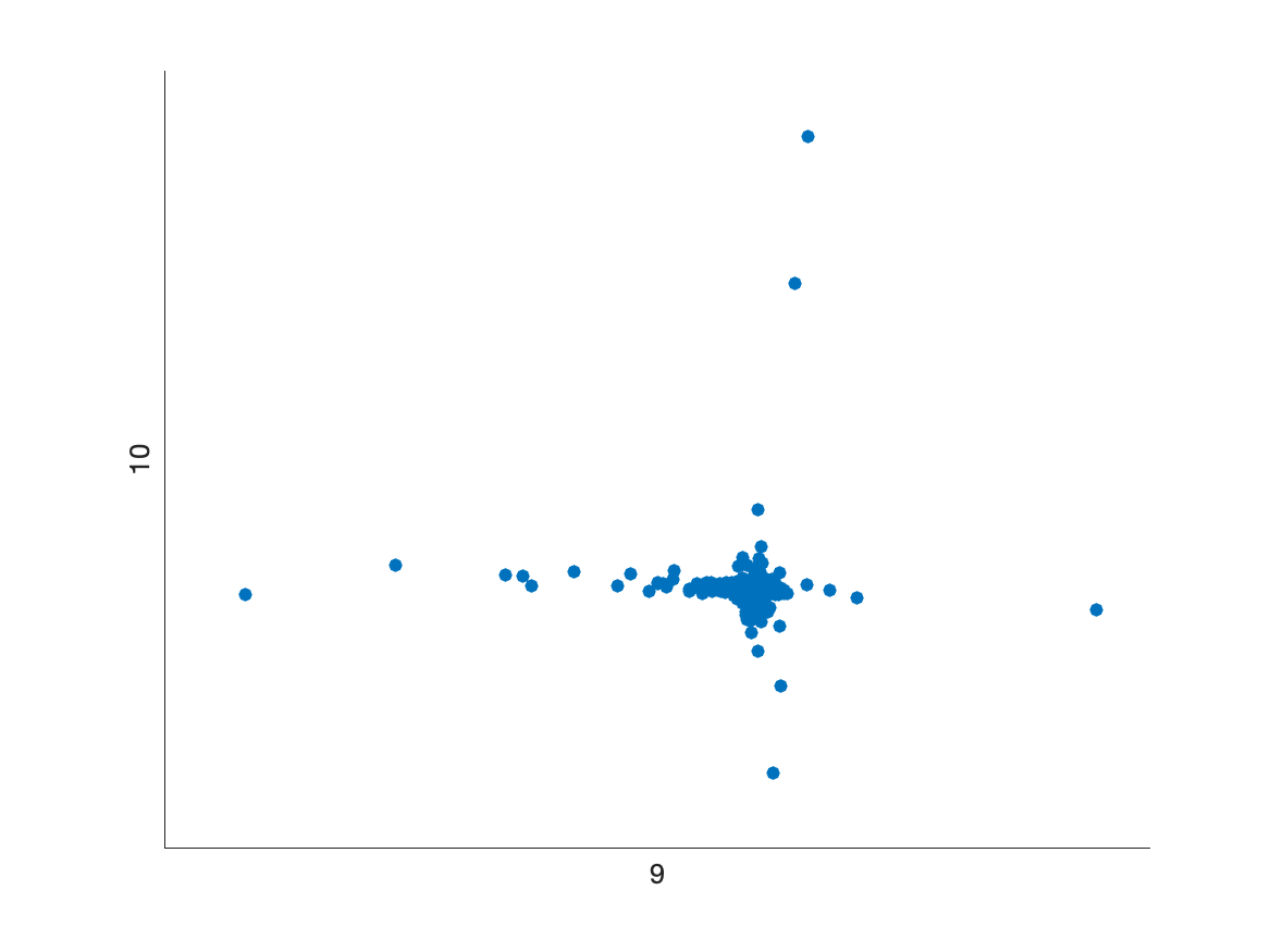
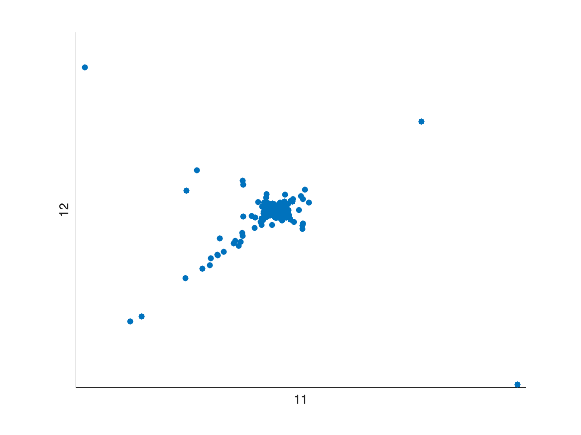
The data has cells, and we include genes from each cell. We preprocess the data matrix by subtracting the mean from each row and normalizing each column. Furthermore, we impute the missing values as zeros. Fig. 10 shows the empirical spectral distribution of this data (i.e., the histogram of its singular values) and the cut-offs chosen by Permutation PA and Signflip PA (with both pairwise comparison and upper-edge comparison). We use trials and a percentile of for all four methods. Permutation PA with pairwise comparison selects 491 components, and using upper-edge comparison selects 128 components. In contrast, Signflip PA with pairwise comparison selects nine, and using upper-edge comparison selects only one. Upper-edge comparison is noticeably more conservative here.
We do not know the ground truth for this real data, but the empirical spectral distribution does appear to have several isolated singular values outside of a “bulk”. In particular, the nine singular values above the cut-off shown for Signflip PA with pairwise comparison. We plot the first twelve left singular vectors of the data in Fig. 11; each point corresponds to a cell. There seems to be some clustering structure in at least the first eight principal components, which somewhat supports the selection made by Signflip PA with pairwise comparison. The selection of one component by Signflip PA with upper-edge comparison is likely overly conservative, and might be the result of insufficient signal destruction leading to an inflated operator norm estimate. Permutation PA with either selection rule is likely selecting too many principal components (the cut-offs are well into the “bulk”). This may be due to heterogeneity in the noise, highlighting the need for flexible approaches that can accommodate potential heterogeneity in the noise.
We also tried several popular non-PA factor selection methods. The eigenvalue ratio method (Ahn and Horenstein, 2013) selected one factor, while the eigenvalue difference method (Onatski, 2010) selected three components. These methods were designed to tackle models with strong factors, so it is perhaps natural that they tend to select relatively fewer components. The information criterion-based estimator (Nadakuditi and Edelman, 2008) selected 2432 components. This method has theoretical guarantees for identifying weak factors, but under a white noise model. A potential reason why it selects so many components (nearly half) may be due to heterogeneity in the noise.
Indeed, much more work is needed to thoroughly assess the performance of these approaches for a suite of real scRNA-seq datasets, which also have additional complexities (e.g., dependent noise). Nevertheless, in this preliminary experiment, we find that Signflip PA appears to be a promising approach. It gave a reasonable estimate of the rank, with its ability to handle heterogeneous noise potentially aiding the selection. Further investigation is beyond the scope of this paper but is an exciting direction for future work!
Acknowledgements
The authors thank Johannes Alt, Andreas Buja, Johannes Heiny, Matthew McKay for helpful and stimulating discussions. They are also grateful to seminar participants at RMCDAW 2019 and Berkeley for feedback on early versions. This work was partially supported by NSF BIGDATA grant IIS 1837992 and the Dean’s Fund for Postdoctoral Research of the Wharton School.
References
- Ahn and Horenstein (2013) S. C. Ahn and A. R. Horenstein. Eigenvalue ratio test for the number of factors. Econometrica, 81(3):1203–1227, 2013.
- Alessi et al. (2010) L. Alessi, M. Barigozzi, and M. Capasso. Improved penalization for determining the number of factors in approximate factor models. Statistics & Probability Letters, 80(23):1806–1813, 2010.
- Anderson (2003) T. W. Anderson. An Introduction to Multivariate Statistical Analysis. Wiley New York, 2003.
- Andrews and Hemberg (2018) T. S. Andrews and M. Hemberg. Identifying cell populations with scrnaseq. Molecular Aspects of Medicine, 59:114 – 122, 2018.
- Apley and Shi (2001) D. W. Apley and J. Shi. A factor-analysis method for diagnosing variability in multivariate manufacturing processes. Technometrics, 43(1):84–95, 2001.
- Bai and Ng (2002) J. Bai and S. Ng. Determining the number of factors in approximate factor models. Econometrica, 70(1):191–221, 2002.
- Bai and Ng (2008) J. Bai and S. Ng. Large dimensional factor analysis. Now Publishers Inc, 2008.
- Bai and Silverstein (2010) Z. Bai and J. W. Silverstein. Spectral analysis of large dimensional random matrices. Springer Series in Statistics. Springer, 2010.
- Bai and Zhou (2008) Z. Bai and W. Zhou. Large sample covariance matrices without independence structures in columns. Statistica Sinica, 18(2):425–442, 2008.
- Bai et al. (2018) Z. Bai, K. P. Choi, Y. Fujikoshi, et al. Consistency of aic and bic in estimating the number of significant components in high-dimensional principal component analysis. Annals of Statistics, 46(3):1050–1076, 2018.
- Baik and Silverstein (2006) J. Baik and J. W. Silverstein. Eigenvalues of large sample covariance matrices of spiked population models. Journal of Multivariate Analysis, 97(6):1382–1408, 2006.
- Baik et al. (2005) J. Baik, G. Ben Arous, and S. Péché. Phase transition of the largest eigenvalue for nonnull complex sample covariance matrices. Annals of Probability, 33(5):1643–1697, 2005.
- Balzano et al. (2010) L. Balzano, R. Nowak, and B. Recht. Online identification and tracking of subspaces from highly incomplete information. In Allerton Conference on Communication, Control, and Computing., pages 704–711. IEEE, 2010.
- Bandeira and Van Handel (2016) A. S. Bandeira and R. Van Handel. Sharp nonasymptotic bounds on the norm of random matrices with independent entries. The Annals of Probability, 44(4):2479–2506, 2016.
- Bartlett (1954) M. S. Bartlett. A note on the multiplying factors for various approximations. Journal of the Royal Statistical Society. Series B (Methodological), 16(2):296–298, 1954.
- Benaych-Georges and Nadakuditi (2012) F. Benaych-Georges and R. R. Nadakuditi. The singular values and vectors of low rank perturbations of large rectangular random matrices. Journal of Multivariate Analysis, 111:120–135, 2012.
- Billingsley (1995) P. Billingsley. Probability and Measure. John Wiley & Sons, 1995.
- Bordenave et al. (2020) C. Bordenave, S. Coste, and R. R. Nadakuditi. Detection thresholds in very sparse matrix completion. arXiv preprint arXiv:2005.06062, 2020.
- Brown (2014) T. A. Brown. Confirmatory factor analysis for applied research. Guilford Publications, 2014.
- Bryson et al. (2019) J. Bryson, R. Vershynin, and H. Zhao. Marchenko-pastur law with relaxed independence conditions. arXiv preprint arXiv:1912.12724, 2019.
- Buja and Eyuboglu (1992) A. Buja and N. Eyuboglu. Remarks on parallel analysis. Multivariate behavioral research, 27(4):509–540, 1992.
- Cai et al. (2020) T. Cai, X. Han, and G. Pan. Limiting laws for divergent spiked eigenvalues and largest non-spiked eigenvalue of sample covariance matrices. The Annals of Statistics, 48(3):1255–1280, 2020.
- Cattell (1966) R. B. Cattell. The scree test for the number of factors. Multivariate Behavioral Research, 1(2):245–276, 1966.
- Cattell and Vogelmann (1977) R. B. Cattell and S. Vogelmann. A comprehensive trial of the scree and kg criteria for determining the number of factors. Multivariate Behavioral Research, 12(3):289–325, 1977.
- Chen and Li (2020) Y. Chen and X. Li. Determining the number of factors in high-dimensional generalised latent factor models. arXiv preprint arXiv:2010.02326, 2020.
- Couillet and Debbah (2011) R. Couillet and M. Debbah. Random Matrix Methods for Wireless Communications. Cambridge University Press, 2011.
- Couillet et al. (2011) R. Couillet, M. Debbah, and J. W. Silverstein. A deterministic equivalent for the analysis of correlated mimo multiple access channels. IEEE Transactions on Information Theory, 57(6):3493–3514, 2011.
- Dobriban (2015) E. Dobriban. Efficient computation of limit spectra of sample covariance matrices. Random Matrices: Theory and Applications, 04(04):1550019, 2015.
- Dobriban (2020) E. Dobriban. Permutation methods for factor analysis and pca. The Annals of Statistics, 48(5):2824–2847, 2020.
- Dobriban (2021) E. Dobriban. Consistency of invariance-based randomization tests. Annals of Statistics, to appear; arXiv preprint arXiv:2104.12260, 2021.
- Dobriban and Owen (2018) E. Dobriban and A. B. Owen. Deterministic parallel analysis: an improved method for selecting factors and principal components. Journal of the Royal Statistical Society. Series B (Methodological), 81(1):163–183, 2018.
- Erdős et al. (2011) L. Erdős, B. Schlein, and H.-T. Yau. Universality of random matrices and local relaxation flow. Inventiones mathematicae, 185(1):75–119, 2011.
- Fan et al. (2014) J. Fan, Q. Sun, W.-X. Zhou, and Z. Zhu. Principal component analysis for big data. Wiley StatsRef: Statistics Reference Online, pages 1–13, 2014.
- Fan et al. (2020) J. Fan, J. Guo, and S. Zheng. Estimating number of factors by adjusted eigenvalues thresholding. Journal of the American Statistical Association, 0(ja):1–33, 2020.
- Fishler et al. (2002) E. Fishler, M. Grosmann, and H. Messer. Detection of signals by information theoretic criteria: general asymptotic performance analysis. IEEE Transactions on Signal Processing, 50(5):1027–1036, 2002.
- Girko (2001) V. L. Girko. Theory of Stochastic Canonical Equations: Volumes I and II. Springer Netherlands, 2001.
- Guionnet and Husson (2020) A. Guionnet and J. Husson. Large deviations for the largest eigenvalue of rademacher matrices. Annals of Probability, 48(3):1436–1465, 2020.
- Hachem et al. (2006) W. Hachem, P. Loubaton, and J. Najim. The empirical distribution of the eigenvalues of a gram matrix with a given variance profile. Annales de l’Institut Henri Poincare (B) Probability and Statistics, 42(6):649–670, 2006.
- Hachem et al. (2008) W. Hachem, P. Loubaton, J. Najim, et al. A clt for information-theoretic statistics of gram random matrices with a given variance profile. The Annals of Applied Probability, 18(6):2071–2130, 2008.
- Hong et al. (2016) D. Hong, L. Balzano, and J. A. Fessler. Towards a theoretical analysis of pca for heteroscedastic data. In 2016 54th Annual Allerton Conference on Communication, Control, and Computing (Allerton), pages 496–503, Sept 2016.
- Hong et al. (2018a) D. Hong, L. Balzano, and J. A. Fessler. Asymptotic performance of pca for high-dimensional heteroscedastic data. Journal of multivariate analysis, 167:435–452, 2018a.
- Hong et al. (2018b) D. Hong, J. A. Fessler, and L. Balzano. Optimally weighted pca for high-dimensional heteroscedastic data. arXiv preprint arXiv:1810.12862, 2018b.
- Horn (1965) J. L. Horn. A rationale and test for the number of factors in factor analysis. Psychometrika, 30(2):179–185, 1965.
- Hui and Pan (2010) J. Hui and G. Pan. Limiting spectral distribution for large sample covariance matrices with m-dependent elements. Communications in Statistics - Theory and Methods, 39(6):935–941, 2010.
- Husson (2020) J. Husson. Large deviations for the largest eigenvalue of matrices with variance profiles. arXiv preprint arXiv:2002.01010, 2020.
- Johnstone (2007) I. M. Johnstone. High dimensional statistical inference and random matrices. In International Congress of Mathematicians. Vol. I, pages 307–333. Eur. Math. Soc., Zürich, 2007.
- Johnstone and Paul (2018) I. M. Johnstone and D. Paul. Pca in high dimensions: An orientation. Proceedings of the IEEE, 106(8):1277–1292, 2018.
- Jolliffe (2002) I. Jolliffe. Principal component analysis. Wiley Online Library, 2002.
- Kaiser (1960) H. F. Kaiser. The application of electronic computers to factor analysis. Educational and Psychological Measurement, 20(1):141–151, 1960.
- Kapetanios (2004) G. Kapetanios. A New Method for Determining the Number of Factors in Factor Models with Large Datasets. Working Papers 525, Queen Mary University of London, School of Economics and Finance, 2004.
- Kapetanios (2010) G. Kapetanios. A testing procedure for determining the number of factors in approximate factor models with large datasets. Journal of Business & Economic Statistics, 28(3):397–409, 2010.
- Ke et al. (2020) T. Ke, Y. Ma, and X. Lin. Estimation of the number of spiked eigenvalues in a covariance matrix by bulk eigenvalue matching analysis. arXiv preprint arXiv:2006.00436, 2020.
- Kritchman and Nadler (2009) S. Kritchman and B. Nadler. Non-parametric detection of the number of signals: Hypothesis testing and random matrix theory. IEEE Transactions on Signal Processing, 57(10):3930–3941, 2009.
- Lam and Yao (2012) C. Lam and Q. Yao. Factor modeling for high-dimensional time series: Inference for the number of factors. The Annals of Statistics, 40(2):694–726, 2012.
- Latała (2005) R. Latała. Some estimates of norms of random matrices. Proceedings of the American Mathematical Society, 133(5):1273–1282, 2005.
- Latała et al. (2018) R. Latała, R. van Handel, and P. Youssef. The dimension-free structure of nonhomogeneous random matrices. Inventiones mathematicae, 214(3):1031–1080, 2018.
- Lawley (1956) D. N. Lawley. Tests of significance for the latent roots of covariance and correlation matrices. Biometrika, 43(1-2):128–136, 1956.
- Leeb (2019) W. Leeb. Matrix denoising for weighted loss functions and heterogeneous signals. arXiv preprint arXiv:1902.09474, 2019.
- Leeb and Romanov (2018) W. Leeb and E. Romanov. Optimal spectral shrinkage and pca with heteroscedastic noise. arXiv preprint arXiv:1811.02201, 2018.
- Lehmann and Romano (2005) E. L. Lehmann and J. P. Romano. Testing statistical hypotheses. Springer Science & Business Media, 2005.
- Lin et al. (2016) Z. Lin, C. Yang, Y. Zhu, J. Duchi, Y. Fu, Y. Wang, B. Jiang, M. Zamanighomi, X. Xu, M. Li, N. Sestan, H. Zhao, and W. H. Wong. Simultaneous dimension reduction and adjustment for confounding variation. Proceedings of the National Academy of Sciences, 113(51):14662–14667, 2016.
- Macosko et al. (2015) E. Z. Macosko, A. Basu, R. Satija, J. Nemesh, K. Shekhar, M. Goldman, I. Tirosh, A. R. Bialas, N. Kamitaki, E. M. Martersteck, J. J. Trombetta, D. A. Weitz, J. R. Sanes, A. K. Shalek, A. Regev, and S. A. McCarroll. Highly parallel genome-wide expression profiling of individual cells using nanoliter droplets. Cell, 161(5):1202–1214, 2015.
- Marchenko and Pastur (1967) V. A. Marchenko and L. A. Pastur. Distribution of eigenvalues for some sets of random matrices. Mat. Sb., 114(4):507–536, 1967.
- McKennan (2020) C. McKennan. Factor analysis in high dimensional biological data with dependent observations. arXiv preprint arXiv:2009.11134, 2020.
- Nadakuditi and Edelman (2008) R. R. Nadakuditi and A. Edelman. Sample eigenvalue based detection of high-dimensional signals in white noise using relatively few samples. IEEE Transactions on Signal Processing, 56(7):2625–2638, 2008.
- Onatski (2010) A. Onatski. Determining the number of factors from empirical distribution of eigenvalues. The Review of Economics and Statistics, 92(4):1004–1016, 2010.
- Owen and Wang (2016) A. B. Owen and J. Wang. Bi-cross-validation for factor analysis. Statistical Science, 31(1):119–139, 2016.
- Papadimitriou et al. (2005) S. Papadimitriou, J. Sun, and C. Faloutsos. Streaming pattern discovery in multiple time-series. In Proceedings of the 31st International Conference on Very Large Data Bases (VLDB), pages 697–708, 2005.
- Passemier and Yao (2014) D. Passemier and J. Yao. Estimation of the number of spikes, possibly equal, in the high-dimensional case. Journal of Multivariate Analysis, 127:173–183, 2014.
- Patil et al. (2010) V. H. Patil, M. Q. McPherson, and D. Friesner. The use of exploratory factor analysis in public health: A note on parallel analysis as a factor retention criterion. American Journal of Health Promotion, 24(3):178–181, 2010.
- Peres-Neto et al. (2005) P. R. Peres-Neto, D. A. Jackson, and K. M. Somers. How many principal components? stopping rules for determining the number of non-trivial axes revisited. Computational Statistics & Data Analysis, 49(4):974–997, 2005.
- Pisier and Xu (2003) G. Pisier and Q. Xu. Non-commutative lp-spaces. Handbook of the geometry of Banach spaces, 2:1459–1517, 2003.
- Seginer (2000) Y. Seginer. The expected norm of random matrices. Combinatorics, Probability and Computing, 9(2):149–166, 2000.
- Serdobolskii (2007) V. I. Serdobolskii. Multiparametric Statistics. Elsevier, 2007.
- Silverstein and Bai (1995) J. W. Silverstein and Z. Bai. On the empirical distribution of eigenvalues of a class of large dimensional random matrices. Journal of Multivariate Analysis, 54(2):175–192, 1995.
- Stewart (1981) D. W. Stewart. The application and misapplication of factor analysis in marketing research. Journal of Marketing Research, 18(1):51–62, 1981.
- Subbarao et al. (1996) C. Subbarao, N. V. Subbarao, and S. N. Chandu. Characterization of groundwater contamination using factor analysis. Environmental Geology, 28:175–180, 1996.
- Tao (2012) T. Tao. Topics in Random Matrix Theory, volume 132. American Mathematical Soc., 2012.
- Tao and Vu (2011) T. Tao and V. Vu. Random matrices: Universality of local eigenvalue statistics. Acta Math., 206(1):127–204, 2011.
- Tran and Formann (2009) U. S. Tran and A. K. Formann. Performance of parallel analysis in retrieving unidimensionality in the presence of binary data. Educational and Psychological Measurement, 69(1):50–61, 2009.
- Velicer (1976) W. F. Velicer. Determining the number of components from the matrix of partial correlations. Psychometrika, 41(3):321–327, 1976.
- Vershynin (2018) R. Vershynin. High-Dimensional Probability. Cambridge University Press, 2018.
- Wang (2012) H. Wang. Factor profiled sure independence screening. Biometrika, 99(1):15–28, 2012.
- Wax and Kailath (1985) M. Wax and T. Kailath. Detection of signals by information theoretic criteria. IEEE Transactions on Acoustics, Speech, and Signal Processing, 33(2):387–392, 1985.
- Wei et al. (2016) M. Wei, G. Yang, and L. Yang. The limiting spectral distribution for large sample covariance matrices with unboundedm-dependent entries. Communications in Statistics - Theory and Methods, 45(22):6651–6662, 2016.
- Yano et al. (2019) K. Yano, Y. Morinaka, F. Wang, P. Huang, S. Takehara, T. Hirai, A. Ito, E. Koketsu, M. Kawamura, K. Kotake, S. Yoshida, M. Endo, G. Tamiya, H. Kitano, M. Ueguchi-Tanaka, K. Hirano, and M. Matsuoka. Gwas with principal component analysis identifies a gene comprehensively controlling rice architecture. Proceedings of the National Academy of Sciences, 116(42):21262–21267, 2019.
- Yao et al. (2015) J. Yao, Z. Bai, and S. Zheng. Large Sample Covariance Matrices and High-Dimensional Data Analysis. Cambridge University Press, 2015.
- Zhang et al. (2018) A. Zhang, T. T. Cai, and Y. Wu. Heteroskedastic pca: Algorithm, optimality, and applications. arXiv preprint arXiv:1810.08316, 2018.
- Zhou (2019) Y.-H. Zhou. A note on cyclic shift permutation testing for large eigenvalues. Stat, 8(1):e257, 2019.
Appendix A Results on signals
In this section, we will prove all remaining results that concern the signals in the signal-plus-noise model. We also denote the Schatten -norm of a matrix by . Letting be the -th largest singular value of , the Schatten -norm is defined as . When , is the operator norm.
We start with the following lemma.
Lemma A.1 (Expected operator norm of signflipped matrices).
A.1 Proof of Lemma A.1
Define the symmetric matrices
and let be a symmetric Gaussian random matrix, i.e., for . Applying (Latała et al., 2018, Theorem 1.1) to yields
| (6) |
where we have used the following bound, which holds for all :
Next, we bound via a result of Latała (2005)
| (7) | ||||
The first equality holds because , the inequality follows by applying Jensen’s inequality to the norm . The final two equalities hold since and , as the singular values of consist of two copies of those of . Combining 6 and 7 and rewriting yields 5, concluding the proof.
A.2 Proof of Theorem 4.1
Let us first prove that the given conditions suffice for convergence. We have that for any matrix , . This follows from
Then, the first condition follows from . For the second condition, it is enough to show that, conditional on , . This follows from equation (5) in Lemma A.1. The third condition is a direct consequence of Theorem 3.1 in Seginer (2000).
Next, we will study the conditions that guarantee . First, we want to show that, for any , and , . A key observation is, borrowing an argument from Latała et al. (2018), that for any ,
Then, we have
which leads to the following bound333This also follows from the noncommutative Khintchine inequality (Pisier and Xu, 2003).
Then, we would like to show that there exists some , such that . It is enough to show . We recall the following bounds:
We also need that and . Indeed
Then, the desired result follows from
Finally, by using the Cauchy-Schwarz inequality, we have
which implies when is uniformly bounded.
For almost sure convergence, notice that, for any real-valued matrix , we have for all . By Markov’s inequality, for any , we have
So, in order to show almost surely, we only need to show that is summable for some . We condition on , use the same result as in (7) for the Schatten norm, and apply (Latała et al., 2018, Theorem 1.1) to , to find
Since holds when , we have . Thus,
which leads to . This finishes the proof.
A.3 Proof of Theorem 4.2
To show convergence, we take in Theorem 4.1, using the sufficient condition
Since and , we have , which proves the claim.
For almost sure convergence, the result follows directly from Theorem 4.1 by taking in the sufficient condition.
A.4 Proof of Corollary 4.3
For showing convergence, from Theorem 4.2, we have . To ensure that this upper bound converges to zero, it is enough if either , or and .
For almost sure convergence, we use
Thus, by the delocalization assumption, we have
The series converges if , thus it is enough to have one of the following conditions:
-
•
, such that ,
-
•
, such that and .
The first condition corresponds to the following region for :
The second condition corresponds to the following region:
which is equivalent to
The second region is a subset of the first one. Thus, we find the condition for almost sure convergence.
A.5 Proof of Theorem 4.4
For convergence, we start with the triangle inequality . From the proof of Theorem 4.2, we have . Hence, is a sufficient condition.
For almost sure convergence, we can first condition on and use the following bound
The first inequality follows by the triangle inequality for . The second inequality is a consequence of Minkowski’s inequality. The last inequality follows from the proof of Theorem 4.1.
A.6 Proof of Corollary 4.5
For convergence, note that and , so the condition from Theorem 4.4 is ensured by , or and .
For almost sure convergence, by using Hölder’s inequality, we have
Then, by using the assumptions, we have
From the proof of Corollary 4.3, suffices for this upper bound to be summable in .
A.7 Proof of Corollary 4.8
Since , we have , which follows from Theorem 4.7. For the other conditions, we have, for any ,
and similarly for all . The desired result follows.
Appendix B Proofs regarding the noise
B.1 Proof of Theorem 4.11
First, the existence of the l.s.d. of is equivalent to the existence of the l.s.d. of , and the existence of the sharp sub-Gaussian Laplace transform implies the existence of all moments. Thus, from Theorem 3.14 of Couillet and Debbah (2011), it follows that the empirical spectral distribution of converges weakly to a deterministic distribution with probability one. Since the entries of also satisfy the above conditions, the same holds for .
Since the largest singular value of equals the largest eigenvalue of the generalized Wigner matrix , the convergence of the leading singular value of follows from Theorem 1.3 of Husson (2020) applied to . While the variance profile of may not satisfy the assumptions directly, this can be resolved by using approximations (see Lemma 6.4 of Husson (2020) and the discussion thereafter). Finally, an identical argument shows that the leading singular values of also converge to the same limit.
B.2 Proof of Proposition 4.12
Since has a sharp sub-Gaussian Laplace transform, we have the upper bound
where we use that , the independence of and , and the moment generating function for the standard normal random variable . On the other hand, by Jensen’s inequality, we have . Thus, . Taken with and , it follows that is a Rademacher random variable.444See Problem 26.7 of Billingsley (1995).
B.3 Proof of Lemma 4.14
Following the proof of Theorem 1.1 of Bai and Zhou (2008), we proceed in three steps:
Recall that where
For any , we also define
Throughout the proof, for fixed , we will write , where are the real and imaginary parts of . Also, we consider a constant such that for all , , .
Step 1. .
Using the notation , we have
where . By using Lemma 2.6 of Silverstein and Bai (1995), we have . Thus, forms a bounded martingale difference sequence and applying the Burkholder inequality (Bai and Silverstein, 2010, Lemma 2.12) yields, for any and for some depending only on ,
By choosing , this implies due to the Borel-Cantelli lemma.
Step 2. , which satisfies 4.
We define the scalars by
Since , it directly follows that , hence and .
Now, by using the resolvent identity , holding for any two invertible square matrices of the same size, we have
where the last line uses that
Taking the trace and dividing by yields
| (8) |
where for ,
with
By using Lemma 2.6 of Silverstein and Bai (1995) and the fact that , we have
| (9) |
Further, we have . Thus, from , 3 by using that all singular values of are bounded by ,
| (10) |
Now recall from (Couillet and Debbah, 2011, Corollary 3.1), that if is the Stieltjes transform of a measure on , then for any , we have
| (11) |
For , by using , , , and that (11) holds for as it is a Stieltjes transform, we have
Thus,
| (12) |
From (9), (10), and (12), since are fixed, we have, uniformly over ,
Hence, from (8), by using that (11) holds for , as it is a Stieltjes transform, and since the bound for is uniform over ,
| (13) |
Next, we have
Since (11) holds for and as they are Stieltjes transforms, from , and from from Step 1, we have
Thus, from (13), we reach
| (14) |
For each fixed , is a bounded sequence. Thus, for any subsequence of the values taken by , there is a subsubsequence of , such that converges to a limit as .
Now, for all and
and thus the functions converge to uniformly over , and over the sequence . Then, from 14, by using that the empirical distribution of converges to the distribution on (on any sequence, in particular on ), we have, on the sequence
Further, we have and . Hence satisfies the equation
| (15) |
We will show in the next step that the solution to 15 is unique. Thus, converges to a limit which is the unique solution to 15. Combining Step 1, we have for any fixed . Finally, applying a standard argument based on Vitali’s convergence theorem (e.g., see the proof of Theorem 2.9 of Bai and Silverstein (2010)) yields for all , where for all , is the unique solution to 15.
B.4 Proof of Theorem 4.13
We first apply Lemma 4.14 to to obtain the limiting distribution of the e.s.d. of . Then, by using that and have the same non-zero eigenvalues, the desired result follows.
Thus, it remains to show satisfies all conditions in Lemma 4.14. First, we have , where in the second term, the expectation is over both the entries of and the random permutations . By symmetry (as is a uniformly random permutations), one can verify that
and
which leads to .
Next, we may write
By using the independence of the coordinates of , as well as the symmetry of , we find
For , we have
Thus,
Similarly, by using we have
By putting these together, we have
For the first term, by using the assumptions that the entries of have uniformly bounded fourth moments and the entries of are uniformly bounded, we have
For the second term, . For the last term, we have . Thus,
Moreover, . Hence, . This finishes the proof.
Appendix C Proofs regarding rank selection
C.1 Proof of Lemma 5.2
We begin with
where the first line uses the triangle inequality and the second line uses Weyl interlacing (e.g., see Chapter 1 of Tao (2012)).
Then, consider Signflip PA with upper-edge comparison. Fix . Since converges to in probability, we have . If the -th factor is perceptible, by definition there is an such that . For this , we have that hence Signflip PA selects this factor. Using a similar argument, we conclude that Signflip PA with upper-edge comparison selects no imperceptible factors. Similarly, we can show the results for Signflip PA with pairwise comparison.
C.2 Proof of Theorem 5.3
We need to verify conditions from Lemma 5.2 for . For the conditions on the noise, we can use Theorem 4.11, as the conditions hold by assumption. The remaining condition for consistency from Lemma 5.2 is to show in probability, for which we only need to show . Applying the unnormalized version of the convergence result from Theorem 4.4 (see the remark after the statement of that result) to , the sufficient conditions are and . We have , and , , from Exercises 2.5.10 and 3.1.4 of Vershynin (2018). This finishes the proof.