On the abrupt change of the maximum likelihood state in a simplified stochastic thermohaline circulation system

Abstract: The maximum likelihood state for a simplified stochastic thermohaline circulation model is investigated. It is shown that a jump occurs for the maximum likelihood state during transitions between two metastable states. The jump helps to explain the mechanism of the abrupt change in the climate systems as revealed by various climate records.

Key words: Maximum likelihood state, climate transition, stochastic thermohaline circulation, abrupt change, interaction between uncertainty and nonlinearity.

It is well known that strong interaction exists between the thermohaline circulation system and the climate system. To understand the mechanism of the abrupt climate change, various methods have been proposed to estimate the likelihood of abrupt change in the thermohaline circulation system. We study the maximum likelihood state of a simplified stochastic thermohaline circulation system. It is shown that jumps occur along transition pathways of the maximum likelihood state. The jump indicates a dramatic change of the salinity in the thermohaline circulation system. This observation is helpful to understand the mechanism of the abrupt change in the climate system.

1 Introduction

Driven by surface buoyancy forcing and pressure differences in the deep ocean, the thermohaline circulation depends heavily on the temperature and salinity of seawater. The thermohaline circulation plays an important role in maintaining the overall energy balance of the Earth [1, 2], and even a small change in the circulation may have a huge impact on the global climate.

Various climate records reveal that the abrupt climate change is highly related to the transition between the equilibrium states of the thermohaline circulation [3]. Note that in deterministic systems, transitions between equilibrium states would not happen without external excitations. Transitions from one equilibrium state to another are often explained from the viewpoint of stochastic models [4, 5, 6]. It is shown [3] that the thermohaline circulation is a nonlinear bistable system subjected to fluctuating environment, and the stochastic freshwater flux can push the thermohaline circulation system to transit from one stable state to another. Some approaches based on past experiences, such as observed climate data [7, 8] or model simulation [9, 10], have been proposed to estimate the likelihood of abrupt change in the thermohaline circulation system.

Hoping to provide some insights into the mechanism of abrupt change of the state in the thermohaline circulation system, we estimate the maximum likelihood state of the system and investigate how it evolves during the transition process from one equilibrium point to the other.

This paper is organized as follows. In section 2, the stochastic thermohaline circulation model is introduced. The maximum likelihood state transition is investigated with the help of simulation results in section 3. Section 4 is the conclusion.

2 A stochastic thermohaline circulation model

One hemisphere thermohaline circulation can be modeled by two vessels of saltwater solution that are connected by advective flow from below and exchange thermal energy and salinity with each other and with the surrounding atmosphere. One vessel represents the high latitudes or north pole with temperature $T_{p}$ and salinity $S_{p}$, the other vessel stands for the low latitudes or equatorial region having temperature $T_{e}$ and salinity $S_{e}$. Each of the vessels is well mixed and has uniform salinity and temperature. But the salinity and temperature between the vessels may not be the same.

The temperature and salinity differences between equatorial and pole regions, defined as $\Delta T\equiv T_{e}-T_{p}$ and $\Delta S\equiv S_{e}-S_{p}$, respectively, are shown to evolve with time by [4]

$$\begin{split}\dfrac{{\rm d}\Delta T}{dt}&=-\dfrac{1}{t_{r}}\left(\Delta T-\theta\right)-Q(\Delta\rho)\Delta T,\\ \dfrac{{\rm d}\Delta S}{dt}&=\dfrac{F}{H}S_{0}-Q(\Delta\rho)\Delta S,\end{split}$$ (1)

where $\Delta\rho$ is the density difference expressed as

$$\Delta\rho=\alpha_{S}(S_{p}-S_{e})-\alpha_{T}(T_{p}-T_{e}),$$ (2)

and $Q(\Delta\rho)$ is the exchange function expressed as

$$Q(\Delta\rho)=\dfrac{1}{t_{d}}+\dfrac{q}{V}\left({\Delta\rho}\right)^{2}.$$ (3)

Following Cessi [4], the values of the dimensional parameters for the thermohaline circulation model (1) are shown in Table 1. With the scaling on temperature difference, salinity difference and time, $x\equiv\dfrac{\Delta T}{\theta},y\equiv\dfrac{\alpha_{S}\Delta S}{\alpha_{T}\theta},t^{\prime}\equiv\dfrac{t}{t_{d}}$, (1) can be rewritten as the following non-dimensional system,

$$\begin{split}\dot{x}&=-\alpha(x-1)-x\left(1+\mu^{2}(x-y)^{2}\right),\\ \dot{y}&=\bar{F}-y\left(1+\mu^{2}(x-y)^{2}\right),\end{split}$$ (4)

where

$$\bar{F}=\dfrac{\alpha_{S}S_{0}t_{d}}{\alpha_{T}\theta H}F,~{}~{}~{}\alpha=\dfrac{t_{d}}{t_{r}},~{}~{}~{}\mu^{2}=\dfrac{t_{d}}{t_{a}},~{}~{}~{}t_{a}=\dfrac{q(\alpha_{T}\theta)^{2}}{V},$$ (5)

the non-dimensional parameter $\alpha$ measures temperature restoring tensity, $\mu^{2}$ the ratio of the diffusion time scale $t_{d}$ and the temperature relaxation time scale $t_{a}$, and $\bar{F}$ the non-dimensional freshwater flux.

Table 1: Parameters of the thermohaline circulation model given by (1)

Parameter	Description	Value	Dimension
$T_{0}$	reference temperature	$5$	${}^{\rm o}{\rm C}$
$S_{0}$	reference salinity	$35$	${\rm psu^{-1}}$
$\rho_{0}$	reference density	$1029$	${\rm Kg~{}m^{-3}}$
$t_{d}$	the diffusion time	219	${\rm yeays}$
$t_{r}$	temperature relaxation time	25	${\rm days}$
$t_{a}$	advection time scale	35	${\rm years}$
$q$	transport coefficient	$8.84\times 10^{11}$	${\rm m^{3}s^{-1}}$
$\alpha_{S}$	salinity coefficient	$7.5$ $\times 10^{-4}$	${\rm psu^{-1}}$
$\alpha_{T}$	thermal expansion coefficient	$1.7\times 10^{-4}$	${}^{\rm o}{\rm C^{-1}}$
$\theta$	meridional temperature difference	$20$	${}^{\rm o}{\rm C}$
$H$	mean ocean depth	$4500$	${\rm m}$
$V$	control volume	$8250\times 4.5\times 300$	${\rm Km}^{3}$

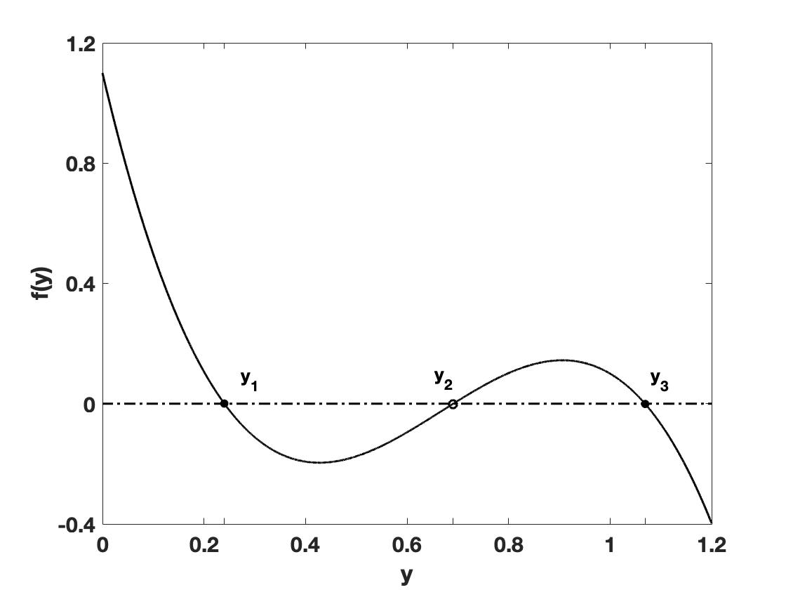
Figure 1: Equilibrium states for deterministic system about salinity difference (6) with freshwater flux $\bar{F}=1.1$ and time scale ratio $\mu^{2}=6.2$.

The system expressed by (4) is a slow-fast dynamical system with $x$ being the fast variable and $y$ the slow variable. Here, only the dynamics of the slow variable $y$ is of interest. It is reasonable to assume that the temperature difference $x$ in the high latitudes is constant for a large $\alpha$ [11]. Therefore, the temperature is clamped to the prescribed value $x=1+\mathcal{O}(\alpha^{-1})$. Consequently, the dynamics for slow variable $y$, the salinity difference between equatorial and pole regions, can be expressed as

$$\dfrac{{\rm d}y}{{\rm d}t}=f(y),$$ (6)

where $f(y)=\bar{F}-y\left(1+\mu^{2}\left(1-y\right)^{2}\right)$.

The equilibrium states are obtained by setting the right hand side of equation (6) equal to zero. With freshwater flux $\bar{F}=1.1$ and time scale ratio $\mu^{2}=6.2$, values for the three equilibrium states are $y_{1}=0.2402$, $y_{2}=0.6911$ and $y_{3}=1.0687$, respectively, as shown in Finger 1.

Now suppose that the freshwater flux $\bar{F}$ has a stochastic component, and consider a stochastic thermohaline circulation model under additive Gaussian noise,

$$\begin{split}{{\rm d}Y(t)}=\left(\bar{F}-Y(t)\left(1+\mu^{2}\left(1-Y(t)\right)^{2}\right)\right){\rm d}t+\epsilon{\rm d}B(t),~{}~{}~{}~{}0<t<T,\end{split}$$ (7)

where $\epsilon$ is noise intensity, $T$ is transition time and $B(t)$ is a standard Brownian motion. This model (7) has been widely used to study the thermohaline circulation under stochastic fluctuations of salinity forcing [3]. Without stochastic fluctuations, i.e. $\epsilon=0$, the salinity difference $y$ always reaches one of the two stable equilibria located at the solid points as shown in Figure 1.

Since this paper is mainly interested in transitions between the two equilibrium states $y_{1}$ and $y_{3}$, (7) is investigated under the following bridge condition,

$$Y(0)=y_{1},~{}~{}~{}~{}Y(T)=y_{3}.$$ (8)

3 Transition of the maximum likelihood state

In this section, we shall study how the maximum likelihood state of (7) under the bridge condition (8) evolves with time. Here the maximum likelihood state at time $t$ for (7) is defined as

$$\psi(t)=\underset{y\in\mathbb{R}}{{\rm arg~{}max}}~{}p(y,t|y_{3},T;y_{1},0),$$ (9)

where $p(y,t|y_{3},T;y_{1},0)$ is the density of $Y(t)$ in (7) at $Y(t)=y$ given $Y(0)=y_{1}$ and $Y(T)=y_{3}$. Note that $\psi(t)$ is the most probable state at time $t$ among all the possible states given the initial and final states.

Let $p(y,t|y_{1},0)$ be the density of $Y(t)$ at $Y(t)=y$ conditioned on $Y(0)=y_{1}$. It satisfies the following forward Fokker-Planck equation [12, 13],

$$\begin{cases}\dfrac{\partial}{\partial t}p(y,t|y_{1},0)=-\dfrac{\partial}{\partial y}\left(\left(\bar{F}-y\left(1+\mu^{2}\left(1-y\right)^{2}\right)\right)p(y,t|y_{1},t_{1})\right)+\dfrac{\epsilon^{2}}{2}p(y,t|y_{1},t_{1}),~{}~{}~{}{\rm for}~{}~{}~{}t>0,\\ ~{}~{}~{}p(y,0|y_{1},0)=\delta(y-y_{1}).\end{cases}$$ (10)

Let $p(y_{3},T|y,t)$ be the density of $Y(t)$ at $Y(t)=y$ conditioned on $Y(T)=y_{3}$. It satisfies the following backward Fokker-Planck equation [13],

$$\begin{cases}\dfrac{\partial}{\partial t}p(y_{3},T|y,t)=-\left(\bar{F}-y\left(1+\mu^{2}\left(1-y\right)^{2}\right)\right)\dfrac{\partial}{\partial y}p(y,t|y_{1},t_{1})-\dfrac{\epsilon^{2}}{2}\dfrac{\partial^{2}}{\partial y^{2}}p(y_{2},T|y,t),~{}~{}~{}{\rm for~{}~{}~{}t<T},\\ ~{}~{}~{}p(y_{3},T|y,T)=\delta(y_{3}-y).\end{cases}$$ (11)

Note that

$$p(y,t|y_{3},T;y_{1},0)=\dfrac{p(y_{2},T|y,t)p(y,t|y_{1},0)}{p(y_{3},T|y_{1},0)},$$ (12)

and $p(y_{3},T|y_{1},0)$ is a constant independent of $y$ and $t$, it follows from (9) and (12) that

$$\psi(t)=\underset{y\in\mathbb{R}}{{\rm arg~{}max}}~{}p(y_{3},T|y,t)p(y,t|y_{1},0).$$ (13)

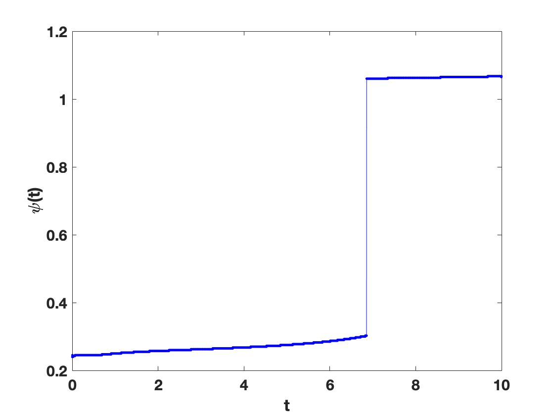
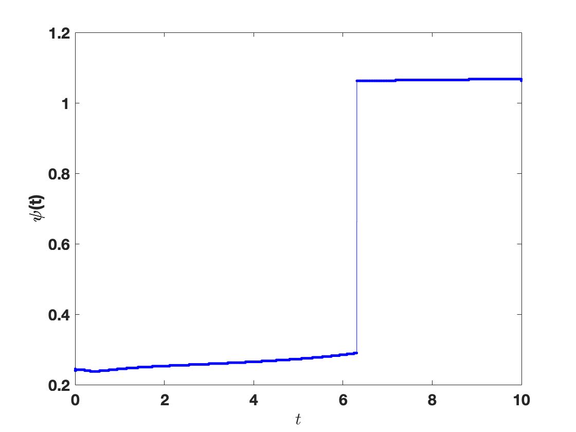
Figure 2: The maximal likelihood transition pathway of stochastic system for salinity difference (7) under condition (8) with freshwater flux $\bar{F}=1.1$, time scale ration $\mu^{2}=6.2$ and noise intensity (a) $\epsilon=0.20$, (b) $\epsilon=0.25$.

The values of $p(y,t|y_{1},0)$ and $p(y_{3},T|y,t)$ in (13) for every $y$ and $t$ can be obtained by numerically solving (10) and (11), respectively. For detailed discuss on the numerical methods for (10) and (11), see [14].

For parameters $\bar{F}=1.1$, $\mu^{2}=6.2$ and noise intensity $\epsilon=0.20,0.25$, the graphs of $\varphi(t)$ are shown in Figure 2 (a) and (b), respectively. It can be seen from the Figure 2 (a) that a jump occurs at $t\approx 6.86$, during the state transition, and the state changes rather slowly before and after the jump, which indicates an abrupt change. As shown in Figure 2 (b), the jump occurs at $t\approx 6.32$. Our simulation shows that the time for the abrupt change is greatly influenced by the strength of the noise. Figure 3 shows how the time of abrupt change varies with noise intensity $\epsilon$. As can be seen from the figure, the abrupt change occurs earlier with the stronger noise.

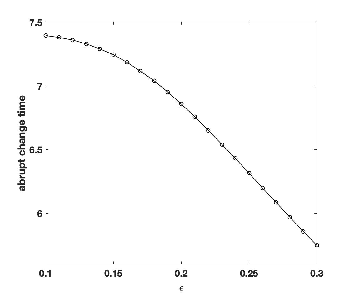
Figure 3: The time for abrupt change $t$ as function of noise intensity $\epsilon$ for stochastic system of salinity difference (7) under the condition $Y(0)=0.2402,$ and $Y(10)=1.0687$.

4 Conclusion

Based on a simplified stochastic thermohaline circulation system, we study how the maximum likelihood state evolves during the transition from one equilibrium state to the other. It is shown, with the help of simulation results, that there is a jump in the transition pathway of the maximum likelihood state. The jump, which indicates an abrupt change for the salinity variability in the thermohaline circulation system, is helpful to understand the abrupt climate change as revealed by various climate records.

Data Availability Statement

The data that support the findings of this study are openly available on GitHub [15].

References

- [1] A. J. Weaver, J. Marotzke, P. F. Cummins, and E. S. Sarachik. Stability and Variability of the Thermohaline Circulation. Journal of Physical Oceanography, 23(1):39–60, 1993.
- [2] A. H. Monahan. Stabilization of Climate Regimes by Noise in a Simple Model of the Thermohaline Circulation. Journal of Physical Oceanography, 32(7):2072–2085, 2002.
- [3] P. Vélez-Belchí, A. Alvarez, P. Colet, J. Tintoré, and R. L. Haney. Stochastic Resonance in the Thermohaline Circulation. Geophysical Research Letters, 28(10):2053–2056, 2001.
- [4] P. Cessi. A Silmple Box Model of Stochastically Forced Thermohaline Flow. Journal of Physical Oceanography, 24(9):1911–1920, 1994.
- [5] A. Timmermann and G. Lohmann. Noise-induced Transitions in a Simplified Model of the Thermohaline Circulation. Journal of Physical Oceanography, 30(8):1891–1900, 2000.
- [6] M. N. Lorenzo, J. J. Taboada, I. Iglesias, and I. Alvarez. The Role of Stochastic Forcing on the Behavior of Thermohaline Circulation. Trends and Directions in Climate Resesrch, 1146:60–86, 2008.
- [7] J. R. Knight, R. J. Allan, C. K. Folland, M. Vellinga, and M. E. Mann. A Signature of Persistent Natural Thermohaline Circulation Cycles in Observed Climate. Geophysical Research Letters, 32(20):L20708, 2005.
- [8] S. Zhang, A. Rosati, and T. Delworth. The Adequacy of Observing Systems in Monitoring the Atlantic Meridional Overturning Circulation and North Atlantic Climate. Journal of Climate, 23(19):5311–5324, 2010.
- [9] E. A. Averyanova, A. B. Polonsky, and V. F. Sannikov. Thermohaline Circulation in the North Atlantic and its Simulation with a Box Model. Izvestiya Atmospheric and Oceanic Physics, 53(3):359–366, 2017.
- [10] S. Rahmstorf. Ocean Circulation and Climate During the Past 120,000 Years. Nature, 419(6903):207–214, 2002.
- [11] H. A. Dijkstra. Nonlinear Climate Dynamics. Cambridge University Press, 2013.
- [12] J. Duan. An Introduction to Stochastic Dynamics. Cambridge University Press, 2015.
- [13] H. Risken and T. Frank. The Fokker-Planck equations: Methods of Solution and Applications. Springer, 1996.
- [14] F. Yang and X. Sun. On Dynamics of the Maximum Likelihood States in Nonequilibrium Systems. Journal of Statistical Physics, 181(3):753–760, 2020.
- [15] F. Yang. Code. Github, 2020. https://github.com/yangfang0914/On-the-abrupt-change-of-the-maximum-likelihood-state-in-a-simplified-stochastic-thermohaline-circula.git.