Does Yoga Make You Happy? Analyzing Twitter User Happiness using Textual and Temporal Information

Abstract

Although yoga is a multi-component practice to hone the body and mind and be known to reduce anxiety and depression, there is still a gap in understanding people’s emotional state related to yoga in social media. In this study, we investigate the causal relationship between practicing yoga and being happy by incorporating textual and temporal information of users using Granger causality. To find out causal features from the text, we measure two variables (i) Yoga activity level based on content analysis and (ii) Happiness level based on emotional state. To understand users’ yoga activity, we propose a joint embedding model based on the fusion of neural networks with attention mechanism by leveraging users’ social and textual information. For measuring the emotional state of yoga users (target domain), we suggest a transfer learning approach to transfer knowledge from an attention-based neural network model trained on a source domain. Our experiment on Twitter dataset demonstrates that there are $1447$ users where “yoga Granger-causes happiness”.

I Introduction

Yoga focuses on the body-mind-spirit connection and its importance in all aspects of personal development and well-being by incorporating a wide variety of postural/exercise, breathing, and meditation techniques [1]. Many studies show that yoga can alleviate symptoms of anxiety and depression as well as promote good physical fitness [2, 3, 4, 5]. The main reason for yoga’s growing popularity [6] is the large-scale transmission of education. Interest in this topic can come from either practitioners or commercial parties. Despite the current popularity of yoga, there is little research on analyzing people’s life-style decision about yoga in social media.

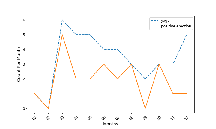
(a) Year 2018

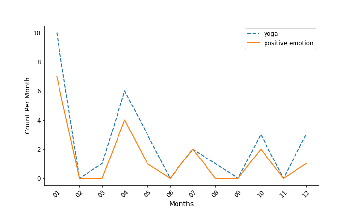
(b) Year 2019.

Figure 1: Example of causal features of a practitioner in two different years. We have two causal features. One is Yoga activity (blue dotted line) and another is Positive emotion (orange solid line).

Nowadays people spend a significant amount of time on social media to express opinions, interact with friends, share ideas and thoughts. As a result, social media data contain rich information providing opportunities to study language and social behavior on a large scale. Leveraging the social media data effectively have been increasingly used to better understand human minds and predict human behavior. Prior research has demonstrated that by analyzing the information in a user’s social media account, we can infer many latent user characteristics like personality [7, 8], emotions [9], mental health [10], mental disorders [11, 12].

Over the past several years, many studies have been devoted towards exploring individual well-being on social media [13, 14, 15, 16]. However, finding causal link between yoga and happiness through the language people use on social media remains unexplored.

In this paper, we find causal relationship between doing yoga and being happy by incorporating textual and temporal information of practitioners using Granger causality [17]. We use well-being related tweets from Twitter focusing on Yoga.

We measure two variables to extract causal features from text. One is yoga activity level based on tweet content analysis and another is happiness level based on the emotional state of practitioner. Fig. 1 shows the example of causal features of a practitioner from our dataset in year $2018$ and $2019$ where we notice a trend between doing yoga and having positive emotion. The causal feature temporally causes rise of positive emotion of the user in March 2018 (Fig. 1(a)) and April 2019 (Fig. 1(b)).

To measure yoga activity level, we predict user type who tweets about yoga whether they are practitioner, promotional, or others i.e. appreciate yoga by tweeting/retweeting about yoga but do not practice yoga. In this work, we propose a method for combining a large amount of Twitter content and social information associated with each user by building a joint embedding attention-based neural network model called Yoga User Network (YUN).

For emotion detection task, we build an attention-based neural network model exploiting the labelled emotion corpus (source domain) collected by reference [18]. As our source task and target task are same, we employ transfer learning approach [19] to detect emotion of yoga practitioners (target domain) focusing on Ekman’s [20] 6 basic emotions (skipping disgust but adding love). We compare our emotion detection model with baseline model which is gated recurrent neural network (GRU) [21] model. For sanity check, we randomly sample $550$ tweets and label them manually with 6 emotions {joy, love, sadness, anger, fear, surprise} as well as including no emotion {ne} tag and calculate accuracy and macro average $F1$-score.

The main contributions of this paper are as follows:

1. We suggest a joint embedding attention-based neural network model called YUN that explicitly learns user embedding leveraging tweet text, emoji, metadata, and user network to classify user type.

2. We evaluate our user type detection model under ten different feature settings: (i) Description; (ii) Location; (iii) Tweets; (iv) Network; (v) BERT (Bidirectional Encoder Representations from Transformers)[22] fine-tuned with Description (Description_BERT); (vi) BERT fine-tuned with Location (Location_BERT); (vii) BERT fine-tuned with Tweets (Tweets_BERT); (viii) joint embedding on description and location (Des + Loc); (ix) joint embedding on description, location, and tweets (Des + Loc + Twt); (x) joint embedding on description, location, and network (Des + Loc + Net). We show that YUN outperforms these settings.

3. We propose an attention-based Bi-directional LSTM model for emotion detection of source domain. We employ transfer learning for emotion detection of yoga practitioners (target domain).

4. We show that our Bi-LSTM attention model outperforms the baseline based on the sanity check.

5. We analyze Granger causality between yoga activity and happiness on Twitter data. Among $8813$ practitioners who tweeted about ‘yoga’ and having positive emotion, we observe that for $1447$ practitioners “yoga Granger-causes happiness”.

Reproducibility: Our code and the data are available at this link Causal-Yoga-Happiness.

The rest of the paper is organized as follows: Section II discusses the relevant literature; Section III provides problem definition of our work; next, Section IV describes the proposed methodology; then, Section V has details of dataset; later, Section VI discusses the baseline models, hyperparameter tuning, and experimental results.

II Related Work

Prior works on causality detection [23, 24, 25] in time series data use Granger causality for predicting future values of a time series using past values of its own and another time series. Our study focuses on the reason to see whether yoga makes people happy by employing Granger causality test using textual and temporal information of the user.

Research on understanding the demographic properties of Twitter users by exploiting user’s community information along with textual features [26, 27, 28, 29, 30] has become increasingly popular. Our main challenge is to use these information to construct a coherent user representation relevant for the specific set of choices that we are interested in. We propose a joint embedding attention-based neural network model which explicitly learns Twitter user representations by leveraging social and textual information of users to understand their types i.e. practitioner, promotional, and others.

Besides, emotion is a key aspect of human life and have a wide array of applications in health and well-being. Early works on emotion detection [31, 32] focused on conceptualizing emotions by following Ekman’s model of six basic emotions: anger, disgust, fear, joy, sadness and surprise [20]. Reference [33] collected a large emotion corpus ($5$ millions) for $5$ of Ekman’s $6$ basic emotions (skipping disgust), but adding love and thankfulness. References [34, 35], and [36] followed the Wheel of Emotion [37] considering emotions as a discrete set of eight basic emotions. Emotion recognition of yoga user still suffers from the bottleneck of labeled data. So we use transfer learning approach to detect emotion of yoga practitioners focusing on six emotions {joy, love, sadness, anger, fear, surprise}.

III Problem Statement

In this section, we define two major parts of our work: A) Find Granger causality, B) Transfer knowledge from source to target.

III-A Granger Causality

Granger causality [17] is a probabilistic account of causality method to investigate causality between two variables in a time series. It is developed in the field of econometric time series analysis. Granger formulated a statistical definition of causality based on the essential assumptions that (i) a cause occurs before its effect and (ii) knowledge of a cause can be used to predict its effect. A time series $X$ (source) is said to Granger-cause a time series $Y$ (target) if past values $x_{t-i}$ are significant indicators in predicting $y_{t}$. So future target value $y_{t}$ depends on both past target time series $y_{t-i}$ and past source time series $x_{t-i}$ rather than only past target time series $y_{t-i}$.

Let’s assume, we compute the Yoga activity level $(a)$ and Happiness level $(p)$. According to Granger causality, given a target time series $p$ (effect) and a source time series $a$ (cause), predicting future target value $p_{t}$ depends on both past target $(p_{<t})$ and past source time series $(a_{<t})$. We calculate Granger causality as follows:

$$GC(p_{t}|p_{<t},a_{<t})=\sum_{i=1}^{m}\alpha_{i}p_{t-i}+\sum_{j=1}^{n}\beta_{j}a_{t-j}$$ (1)

where, $m$ and $n$ are size of lags in the past observation, $\alpha$ and $\beta$ are learnable parameters to maximize the prediction expectation.

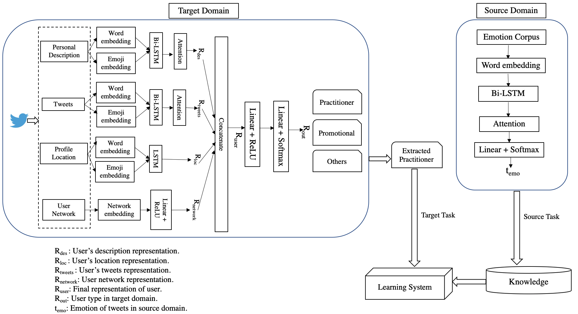
Figure 2: Overall architecture of our work. Inside the target domain (blue box of left-hand side), we have YUN model. YUN has four sub-networks: Description, Location, Tweets, and User Network. Description and Tweets sub-networks use Attention based Bi-LSTM network to generate representation of description, $R_{des}$ and tweets, $R_{tweets}$ respectively. Location sub-network uses only LSTM to create location representation, $R_{loc}$ because the length of sequence for location is shorter. User Network uses linear layer with ReLU activation to compute the representation of user network, $R_{network}$. Concatenation of these four representations generate the final user representation, $R_{user}$ which is fed into a fully connected two-layer classifier activated by ReLU and softmax respectively. Inside the source domain (blue box of right-hand side), we have attention-based Bi-LSTM emotion detection model to classify emotion ($t_{emo}$) of source domain. Transfer learning extracts the knowledge from the source task and applies the knowledge to the target task (classify the emotion of yoga practitioners).

III-B Transfer Knowledge

In our work, given a source domain $D_{src}$ and learning task $T_{src}$, a target domain $D_{tgt}$ and learning task $T_{tgt}$, transfer learning aims to help improve the learning of the target predictive function $f_{T}(.)$ in $D_{tgt}$ using the knowledge in $D_{src}$ and $T_{src}$, where $D_{src}\neq D_{tgt}$ and $T_{src}=T_{tgt}$.

III-B1 Target domain

Our target domain consists of yoga practitioners information. We extract the practitioners using YUN model which employs description, location, yoga-related tweets of users, and user network and then jointly builds a neural network model to generate a dense vector representation for each field and finally concatenates these representations as to the feature for multi-class classification.

To obtain the ground-truth of YUN model, we manually annotate by labeling practitioner as ‘0’, promotional as ‘1’, others as ‘2’ (annotation details in subsection V.A).

In YUN model, each feature is processed by a separate sub-network to generate a feature vector representation $R_{i}$. The output of each sub-networks are feature vectors like $R_{1}\in\mathbb{R}^{d^{1}}$, $R_{2}\in\mathbb{R}^{d^{2}}$ $,....,$ and $R_{N}\in\mathbb{R}^{d^{N}}$ respectively, where $N$ is the number of sub-networks. These feature vectors are then concatenated to build a final user representation $R_{user}$ which is fed into a two-layer classifier consisting of a layer $L_{user}\in\mathbb{R}^{({d^{1}}+{d^{2}}+....+{d^{N}})\times h}$, where $h$ is a model parameter, and a layer $L_{out}\in\mathbb{R}^{h\times l}$, where $l$ is the number of output classes. The final output, $R_{out}$ is fully connected to the output layer and activated by softmax to generate a probability distribution over the classes. The final prediction is computed as follows:

$$R_{out}=softmax(W_{out}Z_{user}+b_{out})$$ (2)

where,

$$Z_{user} =relu(W_{user}R_{user}+b_{user}),$$ (3)

$$R_{user} =R_{1}||R_{2}....||R_{N},$$ (4)

$W_{user}$ & $W_{out}$ are weights and $b_{user}$ & $b_{out}$ are biases. We denote the concatenation operation as $||$.

We use cross-entropy loss as the objective function. Let say, $U$ is the number of users and $l$ is the number of class label, then the cross-entropy loss is as following:

$$CE=-\sum_{i=1}^{U}\sum_{j=1}^{l}y_{i}^{j}log(\hat{y}_{i}^{j})$$ (5)

where $y_{i}$ is the ground-truth of user type and $\hat{y}_{i}$ is the predicted probability vector. So, $\hat{y}_{i}^{j}$ is the probability that user $i$ is a $j$ type of user. We minimize the objective function through Gradient Descent with Adadelta [38].

III-B2 Source domain

The source domain consists of emotion corpus $E_{x}$ labeled with 6 emotions {joy, love, sadness, anger, fear, surprise} where $x$ is total the number of tweets in the corpus. The embeddings of tweets are forwarded to a Bi-LSTM [39] which creates hidden state $h_{i}$ at time-step $i$. To assign important words, we use a context-aware attention mechanism [40] with a weight, $a_{i}$ to each word representation. $t_{emo}$ represents the emotion of tweets.

$$t_{emo} =softmax((W_{t}\times\sum_{i=1}^{x}a_{i}h_{i})+b_{t}),t_{emo}\in\mathbb{R}^{2D},$$ (6)

where

$$a_{i} =\frac{exp(m_{i}c_{h})}{\sum_{t=1}^{x}exp(m_{t}c_{h})},$$ (7)

$$m_{i} =tanh(W_{h}h_{i}+b_{h}),m_{i}\in[-1,1],$$ (8)

and with $W_{t}$ , $W_{h}$ and $c_{h}$ are the layer’s weights and $b_{t}$, $b_{h}$ are the biases. $D$ is the size of each LSTM.

We use cross-entropy loss as the objective function. Let say, $x$ is the number of tweets and $e$ is the number of class label, then the cross-entropy loss is:

$$CE_{emo}=-\sum_{i=1}^{x}\sum_{j=1}^{e}g_{i}^{j}log(\hat{g}_{i}^{j})$$ (9)

where $g_{i}$ is the ground-truth of emotion and $\hat{g}_{i}$ is the predicted probability vector of emotion. So, $\hat{g}_{i}^{j}$ is the probability that tweet $i$ has a $j$ emotion. We minimize the objective function through Gradient Descent with ADAM optimizer [41].

IV Technical Approach

The overall architecture of the proposed model is illustrated in Fig. 2. Our working pipeline follows four key stages including 1) joint-embedding model (YUN) to classify user type, 2) emotion detection model for source domain, 3) transferring the knowledge of source domain to detect emotions in target domain, 4) finding Granger causality.

IV-A YUN Model

YUN is a joint embedding model that uses description, location, tweets, and network for user representation to learn user type.

IV-A1 Tweet Representation

To represent the tweet’s textual content, we use pre-trained word embeddings Word2Vec using Skip-gram architecture [42]. For emoji embeddings, we use Emoji2Vec [43]. The embeddings of text and emoji are then forwarded to an attention based Bi-LSTM model to represent user tweet $R_{tweet}$.

IV-A2 Metadata Representation

In this paper, we focus on two metadata fields i.e. user description and location. For description, embeddings of text and emoji are forwarded to Bi-LSTM. The attention mechanism is employed to provide the final representation of user description $R_{des}$ by implementing same approach followed for $R_{tweet}$.

For user location embedding, embeddings of text and emoji are fed to a LSTM to obtain the representation of user location $R_{loc}\in\mathbb{R}^{D}$, where $D$ is the size of LSTM.

IV-A3 User Network Construction and Network Representation

We construct user network based on $@-$mentions in their tweets [44]. We create an undirected and unweighted graph from interactions among users via retweets and/or mentions. In this graph, nodes are all users in the dataset (both train and test), as well as other external users mentioned in their yoga-related tweets. An undirected and unweighted edge is created between two users if either user mentioned the other. In this work, we do not consider edge weights. In our data, some users mention themselves in their tweets and we delete those edges to avoid self-loop. Also, some users mention an external user multiple times in their tweets and we consider an undirected, unweighted edge between them. In our user network graph, in total, we have $73878$ nodes including all users in the dataset (train and test), as well as other external users mentioned in their tweets and $116085$ edges. To compute node embedding, we use Node2Vec [45]. We generate the embedding of user network and forward to linear layer with ReLU [46] activation function to compute user network representation, $R_{network}$.

IV-A4 User Representation

The final user representation, $R_{user}$ is built by concatenation of the four representations generated from four sub-networks description, location, tweets, and user network respectively. We define $R_{user}$ as follows:

$$R_{user}=R_{des}||R_{loc}||R_{tweets}||R_{network}$$ (10)

Then $R_{user}$ is passed through a fully connected two-layer classifier. The final prediction $R_{out}$ is computed same as eqn.(2).

IV-B Emotion Detection Model

Emotions reflect users’ perspectives towards actions and events. As we do not have ground truth for emotion of our yoga data, we use large emotion corpus ($0.4$ millions) [18] for $5$ of Ekman’s $6$ basic emotions (skipping disgust), but adding love. We use pre-trained word embeddings Word2Vec for tweet embedding and forward the embedding to Bi-LSTM with attention network (described in III.B.2).

Finally, we pass the tweet representation to an one-layer classifier activated by softmax (using eqn.(6)) to detect emotion of the large emotion corpus $(E_{x})$. We refer this model as BiLSTMAttEmo model.

IV-C Transfer Learning

We use transfer learning approach by extracting the knowledge from source task (classify emotion of $E_{x}$ ) and applying the knowledge on target task (classify the emotion of $R_{out}$ if they are yoga practitioners).

IV-D Find Causality

After detecting the practitioner’s emotion, we focus two types of emotion {joy, love} to measure happiness level of each practitioner.

To measure yoga activity level, we focus on each practitioner’s first hand experience based on rule based approach. There are two cases we consider, case (i): Explicitly having First Person Singular Number and First Person Plural Number, case (ii): Implicit first hand experience. For explicit case, if a tweet contains any of these words {“i”, “im”, “i’m”, “i’ve”, “i’d”, “i’ll”, “my”, “me”, “mine”, “myself”, “we”, “we’re”, “we’d”, “we’ll”, “we’ve”, “our”, “ours”, “us”, “ourselves”} with ‘yoga’, we select them as yoga activity.

For case (ii), there are some tweets which don’t explicitly mention First Person Singular Number and First Person Plural Number i.e “feeling peaceful after doing morning yoga”, “loved yesterday’s yoga session #motivational #calm”. We use parts of speech tagging [47] to assign parts of speech to each word. We filter out Second and Third Person Singular and Plural Number. We keep those tweets if there are no Verb 3rd-person singular present form (VBZ) and Proper noun singular (NNP) and Noun plural (NNS) and Proper noun plural(NNPS) and Personal pronoun (PRP) and Possessive pronoun (PRP$) with ‘yoga’ as implicit first hand experience of yoga activity level.

We sort yoga activity level $(a)$ and happiness level $(p)$ increasingly based on DateTime and apply Granger causality (eqn.(1)) with different lags. We choose lags by running the Granger test several times. Our null hypothesis is “yoga activity $(a)$ does not Granger-cause happiness $(p)$”. We reject the null hypothesis if $p$-value is $\leq 0.05$.

V Data

We download yoga-related tweets using Tweepy. We use Twitter streaming API to extract $419608$ tweets sub-sequentially from May to November, 2019 related to yoga containing specific keywords ‘yoga’, ‘yogi’, ‘yogalife’, ‘yogalove’, ‘yogainspiration’, ‘yogachallenge’, ‘yogaeverywhere’, ‘yogaeveryday’, ‘yogadaily’, ‘yogaeverydamnday’, ‘yogapractice’, ‘yogapose’, ‘yogalover’, ‘yogajourney’. We downloaded timeline tweets of $22702$ users and among them $15168$ users have at least a yoga-related tweet in their timelines. We have total $35392177$ tweets.

To pre-process the tweets, we first convert them into lower case, remove URLs then use a tweet-specific tokenizer from NLTK to tokenize them. We do not remove emojis.

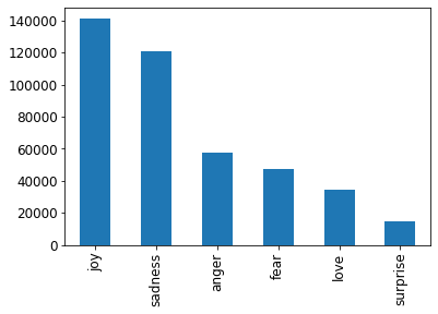
Figure 3: Data distribution of Emotion dataset.

V-A Data Annotation for YUN Model

To run YUN model, we need annotated data. We manually annotated $1300$ users (randomly selected from $15168$ users) based on the intent of the tweets and observation of user description. Consider the following two tweets:

Tweet 1: Learning some traditional yoga with my good friend.

Tweet 2: Our mission at 532Yoga is pretty simple; great teachers, great classes and superbly happy students $\#yoga$

The intention of Tweet 1 is yoga activity (i.e. learning yoga). Tweet 2 is more about promoting a yoga studio. We annotate user of Tweet 1 as practitioner and user of Tweet 2 as promotional.

TABLE I: A summary of hyperparameter settings of the models

Model	lr	opt	reg	word	emoji	unit	attn	h	eut	emo
Description	0.01	Adadelta	0.0001	300	300	150	300	200	23	N/A
Location	0.01	SGD momentum	N/A	300	300	150	300	200	9	N/A
Tweets	0.01	Adadelta	0.0001	300	300	150	300	200	12	N/A
Network	0.01	Adadelta	0.0001	N/A	N/A	N/A	N/A	200	24	N/A
Description_BERT	0.00002	AdamW	0.01	N/A	N/A	N/A	N/A	N/A	4	N/A
Location_BERT	0.00002	AdamW	0.01	N/A	N/A	N/A	N/A	N/A	2	N/A
Tweets_BERT	0.00002	AdamW	0.01	N/A	N/A	N/A	N/A	N/A	2	N/A
Des + Loc	0.01	Adadelta	0.0001	300	300	150	300	200	14	N/A
Des + Loc + Twt	0.01	Adadelta	0.0001	300	300	150	300	200	17	N/A
Des + Loc + Net	0.01	Adadelta	0.0001	300	300	150	300	200	16	N/A
YUN	0.01	Adadelta	0.0001	300	300	150	300	200	18	N/A
GRUEmo	0.001	ADAM	0.0	256	N/A	1024	N/A	N/A	N/A	10
BiLSTMAttEmo	0.01	ADAM	0.0001	300	N/A	150	300	N/A	N/A	21
lr : Learning rate.
opt: Optimizer.
reg : Weight decay ($L^{2}$ regularization).
word: Word embedding dimension.
emoji: Emoji embedding dimension.
unit: LSTM unit size for the models except for GRUEmo model (GRU unit size).
attn: Attention vector size.
h: Size of $L_{user}$ layer which is the first layer of two-layer classifier.
eut: Best result achieved at epochs for user type classification.
eum: Best result achieved at epochs for practitioner’s emotion classification.

V-B Data Distribution for YUN Model

In our user type annotated data ($1300$ users), we have $42\%$ practitioner, $21\%$ promotional, and $37\%$ other users. We shuffle the dataset and then split it into train $(60\%)$, validation $(20\%)$ and test $(20\%)$. We use the trained YUN model to find out the user type of remaining $13860$ users.

V-C Emotion Dataset

The emotion dataset has $0.4$ millions tweets annotated with six emotions {joy, love, sadness, anger, fear, surprise} collected from Twitter using hashtags [18]. The tweets are already pre-processed based on the approach described by reference [18]. The distribution of the data is shown in Fig. 3. We shuffle the dataset and then split it into $60\%$ training, $20\%$ validation and $20\%$ testing data. We use macro average F1-score as the evaluation metric, which is commonly used in emotion recognition studies due to the imbalanced nature of the emotion datasets.

VI Experimental Settings

VI-A Baseline Models

For emotion detection baseline, to represent texts we initialize word embeddings with index mapping for words. We pass this to gated recurrent neural network (GRU) with batch size= $64$ and then forward to an one-layer classifier activated by softmax. We refer this baseline model as GRUEmo model.

TABLE II: Performance comparison of models

	user type detection		emotion detection
Model	Accuracy	Macro avg. F1 score	Accuracy	Macro avg. F1 score
Description	0.725	0.693	N/A	N/A
Location	0.676	0.563	N/A	N/A
Tweets	0.721	0.687	N/A	N/A
Network	0.752	0.557	N/A	N/A
Description_BERT	0.718	0.681	N/A	N/A
Location_BERT	0.679	0.606	N/A	N/A
Tweets_BERT	0.760	0.669	N/A	N/A
Des + Loc	0.733	0.693	N/A	N/A
Des + Loc + Twt	0.760	0.725	N/A	N/A
Des + Loc + Net	0.775	0.723	N/A	N/A
YUN	0.790	0.742	N/A	N/A
GRUEmo	N/A	N/A	0.931	0.90
BiLSTMAttEmo	N/A	N/A	0.923	0.891

In our user type detection model, we explore several combinations of features and evaluate YUN under ten different feature settings as baselines: Description, Location, Tweets, Network, Description_BERT, Location_BERT, Tweets_BERT, Des + Loc, Des + Loc + Twt, Des + Loc + Net.

VI-A1 Description

For user description, to represent texts we initialize word embeddings and emoji embeddings with 300-dimensional pre-trained Word2Vec and Emoji2Vec embeddings correspondingly. We forward these embeddings to Bi-LSTM with attention network to obtain representation of user description. We pass the description representation to a two-layer classifier activated by ReLU and then softmax.

VI-A2 Location

To represent texts we follow same approach like user description. We forward these embeddings to LSTM network to obtain representation of user location. We feed the location representation to a two-layer classifier activated by ReLU and then softmax.

VI-A3 Tweets

For tweets representation, we follow exactly same approach like user description representation.

VI-A4 Network

After constructing user network, we use Node2Vec for network embedding. We forward the network embedding to a linear layer with ReLU activation function for obtaining user network representation. Then We pass the network representation to a two-layer classifier activated by ReLU and softmax respectively.

VI-A5 Des + Loc

We concatenate description and location representations and pass the joint representation to a two-layer classifier activated by ReLU and then softmax.

VI-A6 Des + Loc + Twt

Concatenation of description, location, and tweets representations are fed to the two-layer classifier with ReLU and softmax activation function.

VI-A7 Des + Loc + Net

For this setting, we concatenate description, location, user network representations and forward the joint representation to our two-layer classifier activated by ReLU and softmax respectively.

VI-A8 Description_BERT

We use pre-trained BERT with user description to fine-tune a model to get near state of the art performance in classification. BERT’s input representation is constructed by summing the corresponding token, segment, and position embeddings for a given token. BertForSequenceClassification model with an added single linear layer on top is used for the classification task of user type. As we feed input data, the entire pre-trained BERT model and the additional untrained classification layer is trained on our specific task.

We use the final hidden state of the first token as the input. We denote the vector as $F\in\mathbb{R}^{h}$. Then we add a classifier whose parameter matrix is $W\in\mathbb{R}^{l\times h}$, where $l$ is the number of class label. Finally, the probability $P$ of each class label is calculated by the softmax function $P=softmax(FW^{T})$.

VI-A9 Location_BERT

In this case, we use pre-trained and fine-tuned BertForSequenceClassification model with user location to classify user type.

VI-A10 Tweets_BERT

For Tweets_BERT model, we use pre-trained and fine-tuned BertForSequenceClassification model with user tweets to classify our tasks similar as Description_BERT baseline model.

VI-B Hyperparameter Settings

For all the models except the BERT fine-tuned models, we perform grid hyperparameter search on the validation set using early stopping. For learning rate, we explore values $0.005,0.01,0.05,0.1,0.5$; and for $L^{2}$ regularization, values $0,10^{-4},10^{-3},10^{-2}$. We run the models total $30$ epochs and plot curves for loss and macro-avg F1 score. We set the criteria of early stopping such a way where the validation loss started to increase sharply. In the Description_BERT, Location_BERT, and Tweets_BERT model, to encode our texts, for padding or truncating we decide maximum sentence length = $160,50,500$ respectively. We use batch size = $32$, learning rate = $2e-5$, AdamW optimizer [48], epsilon parameter = $1e-8$, number of epochs = $4$.

Network embeddings are trained using Node2Vec with parameters of dimension $300$, number of walks per source $10$, length of walk per source $80$, minimum count $1$, window size $10$. For users not appearing in the mention network, we set their network embedding vectors as $0$. We pass the network embedding to a linear layer of size $150$ with ReLU activation to compute network representation. Users not having location and/or description, we set the embedding vectors $0$ respectively.

A brief summary of hyperparameter settings of the models is shown in Table I.

VI-C Results

In our experiments, YUN attains the highest test accuracy $(79\%)$ and macro-avg F1 score $(74.2\%)$ for classifying user type. Table II shows the performance comparison of models with baseline on test dataset.

For emotion detection in source task, baseline model GRUEmo achieves $93.1\%$ and $90\%$ test accuracy and macro-avg F1 score respectively (Table II). In that case, our BiLSTMAttEmo has $92.3\%$ test accuracy and $89.1\%$ test macro-avg F1 score (Table II). As the GRUEmo outperforms our BiLSTMAttEmo model for source emotion detection, we transfer knowledge from both model to detect emotion in our target task (emotion detection of yoga practitioners). For sanity check, we randomly sample $550$ tweets and label them manually with {joy, love, sadness, anger, fear, surprise, ne} where {ne} represents no emotion. We calculate accuracy and macro average $F1$-score. We notice that BiLSTMAttEmo model (accuracy = $66.1\%$, macro-avg F1 score = $26.3\%$) performs better in F1 score than GRUEmo model (accuracy = $72.6\%$, macro-avg F1 score = $13.9\%$) for detecting emotion in target task.

TABLE III: Granger causality result for lag = 5

Users	Feature	rn	kn	nc
All	y + h	1663	7120	2271
	y + $1^{st}$ + h	1447	4524	5083
Top $10\%$	y + h	700	399	6
	y + $1^{st}$ + h	546	551	8
rn: Number of users for whom we reject null hypothesis.
kn: Number of users for whom we keep null hypothesis.
nc: Number of users whose Granger Causality is not calculated.
y + h: Yoga and happiness.
y + $1^{st}$ + h: Yoga with $1^{st}$ hand experience and happiness.

We run Granger causality (see subsection III.A) in each practitioner data with different lags = $1,2,3,4,5$. We choose lags by running the Granger test several times. Our null hypothesis is “yoga does not Granger-cause happiness”. We reject the null hypothesis if $p$-value is $\leq 0.05$, otherwise we accept the null hypothesis.

In our case, there are $8813$ practitioners who tweeted about ‘yoga’ and having positive emotion. With lag = $5$, we find that there are $1447$ practitioners for whom “yoga Granger-causes happiness”. For $4524$ practitioners we could not find causation with yoga and happiness. However, for $5083$ practitioners we did not have enough data to calculate Granger causality (Table III).

We select top $10\%$ practitioners who tweeted most about ‘yoga’. After running Granger causality in each of $1105$ practitioners with $5$ lags, we observe that for $546$ practitioners, practicing yoga makes them happy. $551$ practitioners do not have causation with yoga and happiness. Due to the lack of enough data, we could not calculate Granger causality for $8$ practitioners.

Table III shows the combined results of Granger causality test on each practitioner among $15168$ as well as top $10\%$ practitioners ($1105$) based on both features such as ‘yoga + happiness’ and ‘yoga with first hand experience + happiness’. The results are different for those two features because ‘yoga + happiness’ considers all tweets containing ‘yoga’. It does not include practitioner’s first hand experience. On the other hand, ‘yoga with first hand experience + happiness’ feature focuses on yoga activity based on practitioner’s first hand experience (details in subsection IV.D).

To check if the overall activity and happiness of practitioners are temporally correlated, we test Granger causality with the null hypothesis “tweeting more does not Granger-cause positive emotion”. In this case, we have two causal features (i) number of tweets (cause), (ii) number of positive emotions (effect). We calculate Granger causality (similar as equation (1)) with lags = $1,2,3,4,5$ and for each lag, we notice that $p$-value is $>0.05$. So we could not reject the null hypothesis which means the overall activity of the practitioners has no effect on happiness.

As in our work, we did not use contextualized word embedding for text; there are misclassifications among user types. Moreover, our transfer learning approach for the emotion detection of yoga practitioners is noisy. Also, data annotation is expensive. A future direction could be developing a contextualized model to predict user type using minimal supervision and applying a similar approach to detect users’ emotions.

VII Conclusion and Future Work

We analyze the causal relationship between practicing yoga and being happy by leveraging textual and temporal information of Twitter users using Granger causality. To measure two causal features such as (i) understanding user type, we propose a joint embedding attention-based neural network model by incorporating social and textual information of users, (ii) detecting emotion of specific users, we transfer knowledge from attention-based neural network model trained on a source domain. Methodologically, there is more room for improvement, such as our transfer learning approach for emotion is noisy. In future work, we aim to develop a more nuanced way to measure the emotional state of yoga practitioners. We plan to employ the extended version of the proposed methodology in different life-style decision choices i.e. ‘keto diet’, ‘veganism’.

References

- [1] J. R. Goyeche, “Yoga as therapy in psychosomatic medicine,” Psychotherapy and Psychosomatics, vol. 31, no. 1-4, pp. 373–381, 1979.
- [2] S. B. S. Khalsa, “Treatment of chronic insomnia with yoga: A preliminary study with sleep–wake diaries,” Applied psychophysiology and biofeedback, vol. 29, no. 4, pp. 269–278, 2004.
- [3] M. Yurtkuran, A. Alp, and K. Dilek, “A modified yoga-based exercise program in hemodialysis patients: a randomized controlled study,” Complementary therapies in medicine, vol. 15, no. 3, pp. 164–171, 2007.
- [4] K. B. Smith and C. F. Pukall, “An evidence-based review of yoga as a complementary intervention for patients with cancer,” Psycho-Oncology: Journal of the Psychological, Social and Behavioral Dimensions of Cancer, vol. 18, no. 5, pp. 465–475, 2009.
- [5] A. Ross and S. Thomas, “The health benefits of yoga and exercise: a review of comparison studies,” The journal of alternative and complementary medicine, vol. 16, no. 1, pp. 3–12, 2010.
- [6] G. S. Birdee, A. T. Legedza, R. B. Saper, S. M. Bertisch, D. M. Eisenberg, and R. S. Phillips, “Characteristics of yoga users: results of a national survey,” Journal of General Internal Medicine, vol. 23, no. 10, pp. 1653–1658, 2008.
- [7] M. Kosinski, D. Stillwell, and T. Graepel, “Private traits and attributes are predictable from digital records of human behavior,” Proceedings of the national academy of sciences, vol. 110, no. 15, pp. 5802–5805, 2013.
- [8] H. A. Schwartz, J. C. Eichstaedt, M. L. Kern, L. Dziurzynski, S. M. Ramones, M. Agrawal, A. Shah, M. Kosinski, D. Stillwell, M. E. Seligman, et al., “Personality, gender, and age in the language of social media: The open-vocabulary approach,” PloS one, vol. 8, no. 9, p. e73791, 2013.
- [9] Y. Wang and A. Pal, “Detecting emotions in social media: A constrained optimization approach,” in Twenty-fourth international joint conference on artificial intelligence, 2015.
- [10] S. Amir, G. Coppersmith, P. Carvalho, M. J. Silva, and B. C. Wallace, “Quantifying mental health from social media with neural user embeddings,” arXiv preprint arXiv:1705.00335, 2017.
- [11] M. De Choudhury, M. Gamon, S. Counts, and E. Horvitz, “Predicting depression via social media,” in Seventh international AAAI conference on weblogs and social media, 2013.
- [12] A. G. Reece, A. J. Reagan, K. L. Lix, P. S. Dodds, C. M. Danforth, and E. J. Langer, “Forecasting the onset and course of mental illness with twitter data,” Scientific reports, vol. 7, no. 1, p. 13006, 2017.
- [13] H. A. Schwartz, M. Sap, M. L. Kern, J. C. Eichstaedt, A. Kapelner, M. Agrawal, E. Blanco, L. Dziurzynski, G. Park, D. Stillwell, et al., “Predicting individual well-being through the language of social media,” in Biocomputing 2016: Proceedings of the Pacific Symposium, pp. 516–527, World Scientific, 2016.
- [14] H. A. Schwartz, J. C. Eichstaedt, M. L. Kern, L. Dziurzynski, R. E. Lucas, M. Agrawal, G. J. Park, S. K. Lakshmikanth, S. Jha, M. E. Seligman, et al., “Characterizing geographic variation in well-being using tweets.,” ICWSM, vol. 13, pp. 583–591, 2013.
- [15] C. Yang and P. Srinivasan, “Life satisfaction and the pursuit of happiness on twitter,” PloS one, vol. 11, no. 3, p. e0150881, 2016.
- [16] T. Islam, “Yoga-veganism: Correlation mining of twitter health data,” arXiv preprint arXiv:1906.07668, 2019.
- [17] C. W. Granger, “Some recent development in a concept of causality,” Journal of econometrics, vol. 39, no. 1-2, pp. 199–211, 1988.
- [18] E. Saravia, H.-C. T. Liu, Y.-H. Huang, J. Wu, and Y.-S. Chen, “Carer: Contextualized affect representations for emotion recognition,” in Proceedings of the 2018 Conference on Empirical Methods in Natural Language Processing, pp. 3687–3697, 2018.
- [19] S. J. Pan and Q. Yang, “A survey on transfer learning,” IEEE Transactions on knowledge and data engineering, vol. 22, no. 10, pp. 1345–1359, 2009.
- [20] P. Ekman, “An argument for basic emotions,” Cognition & emotion, vol. 6, no. 3-4, pp. 169–200, 1992.
- [21] K. Cho, B. Van Merriënboer, D. Bahdanau, and Y. Bengio, “On the properties of neural machine translation: Encoder-decoder approaches,” arXiv preprint arXiv:1409.1259, 2014.
- [22] J. Devlin, M.-W. Chang, K. Lee, and K. Toutanova, “Bert: Pre-training of deep bidirectional transformers for language understanding,” arXiv preprint arXiv:1810.04805, 2018.
- [23] H. Qiu, Y. Liu, N. A. Subrahmanya, and W. Li, “Granger causality for time-series anomaly detection,” in 2012 IEEE 12th international conference on data mining, pp. 1074–1079, IEEE, 2012.
- [24] S. Acharya, “Causal modeling and prediction over event streams,” 2014.
- [25] D. Kang, V. Gangal, A. Lu, Z. Chen, and E. Hovy, “Detecting and explaining causes from text for a time series event,” arXiv preprint arXiv:1707.08852, 2017.
- [26] J. Li, A. Ritter, and D. Jurafsky, “Learning multi-faceted representations of individuals from heterogeneous evidence using neural networks,” arXiv preprint arXiv:1510.05198, 2015.
- [27] A. Benton, R. Arora, and M. Dredze, “Learning multiview embeddings of twitter users,” in Proceedings of the 54th Annual Meeting of the Association for Computational Linguistics (Volume 2: Short Papers), pp. 14–19, 2016.
- [28] Y. Yang and J. Eisenstein, “Overcoming language variation in sentiment analysis with social attention,” Transactions of the Association for Computational Linguistics, vol. 5, pp. 295–307, 2017.
- [29] P. Mishra, H. Yannakoudakis, and E. Shutova, “Neural character-based composition models for abuse detection,” arXiv preprint arXiv:1809.00378, 2018.
- [30] M. Del Tredici, D. Marcheggiani, S. S. i. Walde, and R. Fernández, “You shall know a user by the company it keeps: Dynamic representations for social media users in nlp,” arXiv preprint arXiv:1909.00412, 2019.
- [31] C. O. Alm, D. Roth, and R. Sproat, “Emotions from text: machine learning for text-based emotion prediction,” in Proceedings of human language technology conference and conference on empirical methods in natural language processing, pp. 579–586, 2005.
- [32] C. Strapparava and R. Mihalcea, “Semeval-2007 task 14: Affective text,” in Proceedings of the Fourth International Workshop on Semantic Evaluations (SemEval-2007), pp. 70–74, 2007.
- [33] W. Wang, L. Chen, K. Thirunarayan, and A. P. Sheth, “Harnessing twitter” big data” for automatic emotion identification,” in 2012 International Conference on Privacy, Security, Risk and Trust and 2012 International Confernece on Social Computing, pp. 587–592, IEEE, 2012.
- [34] J. Suttles and N. Ide, “Distant supervision for emotion classification with discrete binary values,” in International Conference on Intelligent Text Processing and Computational Linguistics, pp. 121–136, Springer, 2013.
- [35] R. Meo and E. Sulis, “Processing affect in social media: A comparison of methods to distinguish emotions in tweets,” ACM Transactions on Internet Technology (TOIT), vol. 17, no. 1, pp. 1–25, 2017.
- [36] M. Abdul-Mageed and L. Ungar, “Emonet: Fine-grained emotion detection with gated recurrent neural networks,” in Proceedings of the 55th annual meeting of the association for computational linguistics (volume 1: Long papers), pp. 718–728, 2017.
- [37] R. Plutchik, “A general psychoevolutionary theory of emotion,” in Theories of emotion, pp. 3–33, Elsevier, 1980.
- [38] M. D. Zeiler, “Adadelta: an adaptive learning rate method,” arXiv preprint arXiv:1212.5701, 2012.
- [39] S. Hochreiter and J. Schmidhuber, “Long short-term memory,” Neural computation, vol. 9, no. 8, pp. 1735–1780, 1997.
- [40] D. Bahdanau, K. Cho, and Y. Bengio, “Neural machine translation by jointly learning to align and translate,” arXiv preprint arXiv:1409.0473, 2014.
- [41] D. P. Kingma and J. Ba, “Adam: A method for stochastic optimization,” arXiv preprint arXiv:1412.6980, 2014.
- [42] T. Mikolov, K. Chen, G. Corrado, and J. Dean, “Efficient estimation of word representations in vector space,” 2013.
- [43] B. Eisner, T. Rocktäschel, I. Augenstein, M. Bošnjak, and S. Riedel, “emoji2vec: Learning emoji representations from their description,” arXiv preprint arXiv:1609.08359, 2016.
- [44] A. Rahimi, D. Vu, T. Cohn, and T. Baldwin, “Exploiting text and network context for geolocation of social media users,” arXiv preprint arXiv:1506.04803, 2015.
- [45] A. Grover and J. Leskovec, “node2vec: Scalable feature learning for networks,” in Proceedings of the 22nd ACM SIGKDD international conference on Knowledge discovery and data mining, pp. 855–864, 2016.
- [46] V. Nair and G. E. Hinton, “Rectified linear units improve restricted boltzmann machines,” in Proceedings of the 27th international conference on machine learning (ICML-10), pp. 807–814, 2010.
- [47] K. Toutanova, D. Klein, C. D. Manning, and Y. Singer, “Feature-rich part-of-speech tagging with a cyclic dependency network,” in Proceedings of the 2003 conference of the North American chapter of the association for computational linguistics on human language technology-volume 1, pp. 173–180, Association for Computational Linguistics, 2003.
- [48] I. Loshchilov and F. Hutter, “Decoupled weight decay regularization,” arXiv preprint arXiv:1711.05101, 2017.