Joint AGC and Receiver Design for Large-Scale MU-MIMO Systems Using Low-Resolution Signal Processing in C-RANs

Abstract

Large-scale multi-user multiple-input multiple-output (MU-MIMO) systems and cloud radio access networks (C-RANs) are considered promising technologies for the fifth generation (5G) of wireless networks. In these technologies, the use of low-resolution analog-to-digital converters (ADCs) is key for energy efficiency and for complying with constrained fronthaul links. Processing signals with few bits implies a significant performance loss and, therefore, techniques that can compensate for quantization distortion are fundamental. In wireless systems, an automatic gain control (AGC) precedes the ADCs to adjust the input signal level in order to reduce the impact of quantization. In this work, we propose the joint optimization of the AGC, which works in the remote radio heads (RRHs), and a low-resolution aware (LRA) linear receive filter based on the minimum mean square error (MMSE), which works in the cloud unit (CU), for large-scale MU-MIMO systems with coarsely quantized signals. We develop linear and successive interference cancellation (SIC) receivers based on the proposed joint AGC and LRA MMSE (AGC-LRA-MMSE) approach. An analysis of the achievable sum rates along with a computational complexity study is also carried out. Simulations show that the proposed AGC-LRA-MMSE design provides substantial gains in bit error rates and achievable information rates over existing techniques.

I Introduction

In recent years, the widespread use of smartphones and bandwidth-intensive applications and services has led to an exponential traffic growth in wireless networks [1]. 5G has been developed to cope with this growth and, at the same time, minimize the network capital and operating expenditures [2, 3]. In order to achieve a substantial increase in capacity, spectral and energy efficiencies, and in average cell throughput, solutions such as cloud radio access networks (C-RANs) and large-scale MU-MIMO will be jointly deployed in the next generation systems [4].

In the traditional cellular network model, each base station (BS) covers a cell, receives, processes and transmits signals to and from the users [5]. In the future, the huge number of devices connected to such networks will require the deployment of more BSs to meet the growing traffic demand. However, the deployment of more BSs results in the increase of inter-cell interference and power consumption due to the BSs’ hardware and cooling systems. In this context, C-RANs are a promising network architecture that performs centralized processing for next-generation systems [6, 7, 8, 9, 11, 12, 10]. In this centralized architecture, BSs are broken down into low-cost Remote Radio Heads (RRHs) and a pool of Base Band Units (BBUs) located within a cloud unit (CU) [10, 9]. The RRHs consist of simple radio antennas and active radio frequency components that perform transmit/receive signal processing such as frequency conversion, power amplification and Analog-to-Digital (A/D) or Digital-to-Analog (D/A) conversion [6]. The signal processing tasks of each BS are migrated to the BBU pool, which is responsible for all the baseband signal processing [12]. Centralization aids network coordination and management, and can bring benefits such as reduction in the cost of operating the network due to fewer site visits, energy consumption due to hardware and air-conditioning and easy upgrades [7]. C-RANs have received a great deal of attention in recent years thanks to their ability to improve the network performance with joint signal processing techniques that span multiple base stations. Therefore, it mitigates the inter-cell interference in an efficient way, and in turn, allowing for higher spectral efficiency (SE)[8]. However, one of the main challenges to implement C-RANs is the limited capacity of fronthaul (FH) links [10, 11].

Large-scale MU-MIMO systems can provide substantial gains over small-scale MU-MIMO systems in both energy and spectral efficiency [13]. In such systems a large number of antennas is employed at the BS to exploit the degrees of freedom and reduce the transmit power per antenna. However, the large number of antennas increases considerably the hardware cost and the power consumption due to the presence of A/D converters (ADCs) and D/A converters (DACs) [14, 15, 22]. The power consumption in an uplink receiver design is heavily dependent on the ADCs processing unit and the digital baseband processing unit, which are both affected by the resolution in bits of the ADCs. Specifically, the ADCs’ power consumption scales linearly in the sampling rate and exponentially in the number of bits [14]. Thus, we can reduce the power consumption at the receiver using low-resolution ADCs. Furthermore, the adoption of ADCs with fewer bits allows reduction in power consumption, faster signal processing, cheaper systems, and alleviates the capacity bottleneck of FH by reducing the number of bits prior to transmission.

Quantizing signals with a low number of bits reduces the signal quality due to the severe nonlinear distortion introduced. In [20, 21, 22, 23] the quantization process is shown to increase the MSE on the channel estimation at the receiver. The quantization error can be categorized into two types of distortions, the granular distortion, and the clipping or overload distortion [18, 17]. The granular distortion occurs when the input signal lies within the quantizer-permitted range. The overload distortion happens when the input signal exceeds the allowed range, resulting in the clipping of the input signal. In practice, ADCs are usually preceded by an AGC variable gain amplifier, which aims to minimize the overload distortion [19] or the effects of a too small input signal. The AGC adjusts the analog signal level to the dynamic range of the ADCs, which is important in scenarios where the received power varies over time such as in mobile systems. In [24] the effects of choosing an adequate output of an AGC prior to quantization are analyzed. Therefore, the AGC is an essential building block in the receiver chain that implies an ADC because otherwise the ADC most likely operates in a suboptimal operating point and, in particular, the AGC design is key in large-scale MU-MIMO systems which employ low-resolution ADCs.

The distortion produced by the quantization process and its impact on the performance of communication systems has been studied in the literature [14, 15, 22, 18, 17, 19, 21, 22, 23, 24, 25, 26, 27, 28, 29, 30, 33, 20, 31, 32, 34]. Nevertheless, few studies address the design of AGCs. In [21] and [23], modified MMSE receivers that take into account the quantization effects in a MIMO system are presented but they do not take into account the presence of an AGC. The effects of a deterministic AGC on a quantized MIMO system with a standard Zero-Forcing receive filter at the receiver were examined in [24]. However, the work in [24] has not optimized the AGC nor used a detector that considers the quantization effects. Moreover, neither [21, 23] nor [24] have been designed for large-scale MU-MIMO with C-RANs. In [14] a suboptimal choice of the set of quantization labels and thresholds was proposed with a rescheduling scheme of the set of labels found through the Lloyd-Max algorithm. This analysis avoids the use of an AGC but the Lloyd-Max algorithm requires the probability density function of the received signal to compute the optimum set of labels, which is not practical. Therefore, novel techniques to deal with the quantization effects for C-RANs are required.

In this work, we develop an uplink framework for jointly designing the AGCs that work in the RRHs and low-resolution aware (LRA) linear receive filters according to the MMSE criterion that works in the CU. We then propose a joint AGC and LRA MMSE (AGC-LRA-MMSE) design approach based on alternating optimization that adjusts the parameters of the AGC and the receive filter. Based on the AGC-LRA-MMSE aproach we then devise linear and SIC receivers. SIC is a well-known layered detection scheme where a symbol is detected at each layer [35, 36, 37, 38]. SIC detection improves the detection accuracy and thus can help the receiver to achieve a good performance even when dealing with coarsely quantized signals. Unlike existing approaches with deterministic AGCs [24] and modified MMSE receive filters [24, 21, 23], the proposed AGC-LRA-MMSE approach jointly optimizes the AGCs and the receive filters based on a statistical criterion using alternating optimization. We report in [34] optimistic results of the proposed joint optimization of the AGC and linear receivers in a MU-MIMO scenario. However, [34] does not consider the SIC detection scheme, the imperfect CSI, the imperfect knowledge about the AGC coefficients at the CU, and does not evaluate the performance of the proposed technique in a large-scale MU-MIMO system in C-RANs that are considered by this paper. We also derive expressions for the achievable sum rates and evaluate the computational complexity of the proposed AGC-LRA-MMSE approach. Simulations show that the proposed AGC-LRA-MMSE design provides substantially better error rates and higher achievable rates than existing techniques. The main contributions of this work can be summarized as:

1. An uplink framework for jointly designing MMSE-based AGCs that work in the RRHs and LRA linear receivers.

2. Linear and SIC receivers based on the proposed AGC-LRA-MMSE approach.

3. Analytical expressions for the achievable sum rates and the computational complexity of the proposed AGC-LRA-MMSE approach.

The organization of this paper is as follows. The next section details the system model of the large-scale MU-MIMO system with the C-RAN signal processing scheme, states the problem and describes the properties of the quantizer adopted and a model for the distortion produced by the quantization process. The proposed AGC-LRA-MMSE design approach is presented along with the details of its derivation and computational complexity in Section III. Section IV develops the sum rate analysis of the proposed AGC-LRA-MMSE approach. Simulation results are presented and discussed in Section V. The conclusions of this paper are given in Section VI.

Notation: Vectors and matrices are denoted by lower and upper case italic bold letters. The operators $(\cdot)^{T}$, $(\cdot)^{H}$ and $\mathop{\rm tr}(\cdot)$ stand for transpose, Hermitian transpose and trace of a matrix, respectively. $\mathbf{1}$ denotes a column vector of ones and $\mathbf{I}$ denotes an identity matrix. The operator $\mathrm{E}[\cdot]$ stands for expectation with respect to the random variables and the operator $\odot$ corresponds to the Hadamard product. Finally, $\mathop{\rm diag}(\mathbf{A})$ denotes a diagonal matrix containing only the diagonal elements of $\mathbf{A}$ and $\mathop{\rm nondiag}(\mathbf{A})=\mathbf{A}-\mathop{\rm diag}(\mathbf{A})$. The operators $\mbox{Q}(\cdot)$ and $\mathrm{DEC}(\cdot)$ represent respectively the quantization of a vector with an arbitrary number of bits and the slicer used for detection.

II System Description

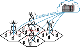
Figure 1: Large-scale MU-MIMO uplink system with centralized signal processing.

Let us consider the uplink of a large-scale MU-MIMO system with C-RANs. As shown in Fig. 1, the system consists of one BBU pool located at the CU and one cluster with $L$ cells in which each cell has one RRH at the center of the cell and a total of $K$ users randomly distributed in their covered area. It is assumed that each RRH is equipped with $N_{R}$ receive antennas, while each user is equipped with $N_{T}$ transmit antennas. It is further assumed that each RRH is connected to the CU via an imperfect finite-capacity digital FH link.

In the uplink, all users simultaneously communicate with the RRHs in the same time-frequency resource. After that, each RRH processes the signal received from all users with independent AGCs, quantizes the AGC output signal and then forwards the quantized signal and also AGC coefficients to the CU via their FH link. Since FH links have high capacity and the number of coefficients is equal to the number of antennas times the number of bits per coefficient, then the load can be considered modest. At last, the BBU pool jointly detects the users’ messages based on signals from all RRHs. The steps of the proposed joint AGC and LRA-MMSE detection scheme are summarized in Algorithm 1.

Algorithm 1 AGC and LRA-MMSE scheme

1:Each RRH receives the analog signals transmitted by all users of the cluster.

2:The $l$-th RRH computes its optimal AGC coefficients.

3:The analog signal received at the $l$-th RRH is sampled, processed by the AGC and then is quantized with few bits of resolution.

4:The quantized signals and the AGC coefficients are sent to the CU through imperfect FH links.

5:Due to the transmission errors in the FH links, the optimal AGC coefficients are assumed to be distorted.

6:The LRA-MMSE receive filter is computed at the CU taking into account the quantization distortion and the presence of the AGCs at the RRHs.

7:The symbols of the users are estimated at the CU by linear or SIC detection schemes.

As the users transmit their signals in the same time-frequency resource, such signals can interfere with each other resulting in the intracell interference and in the intercell interference. In order to model this scenario the $N_{R}$-dimensional received signal vector at the $l$-th RRH can be expressed as

$$\mathbf{y}_{l}=\underbrace{\mathbf{H}_{ll}^{(k)}\mathbf{x}_{l}^{(k)}}_{\stackrel{{\scriptstyle\mathop{\rm desired}}}{{\mathop{\rm signal}}}}+\underbrace{\sum_{\stackrel{{\scriptstyle u=1}}{{u\neq k}}}^{K}\mathbf{H}_{ll}^{(u)}\mathbf{x}_{l}^{(u)}}_{\stackrel{{\scriptstyle\mathop{\rm intracell}}}{{\mathop{\rm interference}}}}+\underbrace{\sum_{\stackrel{{\scriptstyle i=1}}{{i\neq l}}}^{L}\sum_{u=1}^{K}\mathbf{H}_{li}^{(u)}\mathbf{x}_{i}^{(u)}}_{\stackrel{{\scriptstyle\mathop{\rm intercell}}}{{\mathop{\rm interference}}}}+\mathbf{n}_{l},$$ (1)

where $\mathbf{H}_{li}^{(u)}\in\mathbb{C}^{N_{R}\times N_{T}}$ is the channel matrix between the $N_{T}$ transmit antennas of the $u$-th user in the $i$-th cell and the $N_{R}$ receive antennas of the $l$-th RRH; $\mathbf{x}_{i}^{(u)}\in\mathbb{C}^{N_{T}\times 1}$ is the transmitted vector by the $u$-th user in the $i$-th cell; and $\mathbf{n}_{l}\in\mathbb{C}^{N_{R}\times 1}$ contains additive white Gaussian noise (AWGN) at the $l$-th RRH. The elements of both $\mathbf{x}_{i}^{(u)}$ and $\mathbf{n}_{l}$ are assumed to be independent and identically distributed (i.i.d) zero mean circularly symmetric complex Gaussian (ZMCSCG) random variables with variances equal to unit and $\sigma_{n}^{2}$, respectively.

The channel matrix $\mathbf{H}_{li}^{(u)}$ models independent fast fading, geometric attenuation, and log-normal shadow fading [33, 39, 40, 41]. Under perfect channel state information at the receiver (CSIR) assumption, the coefficients of the channel matrix are given by $\mathbf{H}_{li}^{(u)}=\tilde{\mathbf{H}}_{li}^{(u)}\sqrt{\beta_{li}^{(u)}}$, where each entry $\tilde{h}_{limn}^{(u)}$ of $\tilde{\mathbf{H}}_{li}^{(u)}$ represents the fast fading coefficient between the $n$-th transmit antenna of the $u$-th user in the $i$-th cell to the $m$-th receive antenna of the $l$-th RRH. Its coefficients are assumed to be i.i.d ZMCSCG random variables with unit variance. The quantity $\beta_{li}^{(u)}$ represents the geometric attenuation and shadow fading, which is assumed to be independent over $m$ and $n$. This factor is modeled as follows

$$\beta_{li}^{(u)}=\frac{z_{li}^{(u)}}{\left(d_{li}^{(u)}\right)^{\gamma}},$$ (2)

where $z_{li}^{(u)}$ represents the shadow fading and obeys a log-normal distribution with standard deviation $\sigma_{\text{shadow}}$ (i.e, $10\log\left(z_{li}^{(u)}\right)$ follows a Gaussian distribution with zero-mean and standard deviation $\sigma_{\text{shadow}}$), $d_{li}^{(u)}$ corresponds to the distance between the $u$-th user in the $i$-th cell and the RRH in the $l$-th cell measured in kilometers, and $\gamma$ is the path-loss exponent.

In this work we consider a time block fading model where the small-scale channel matrix $\tilde{\mathbf{H}}_{li}^{(u)}$ stays constant during the coherence interval of a data packet, and the large-scale coefficient $\beta_{li}^{(u)}$ stays constant during a large scale coherence interval of a block of data packets [42]. A usual assumption is that one block of data packets corresponds to a set of 40 data packets, i.e, 40 sets of symbols of a given modulation scheme. The matrices $\tilde{\mathbf{H}}_{li}^{(u)}$ and the coefficients $\beta_{li}^{(u)}$ are assumed to be independent in different coherence intervals and large scale coherence intervals, respectively.

In practice, CSI is obtained through channel estimation and thus is inevitably contaminated by noise. The imperfect CSI at the RRH can be modeled through a Gauss-Markov uncertainty of the form [31, 32]

$$\hat{\mathbf{H}}_{\mathrm{est}}=\sqrt{1-\eta^{2}}\tilde{\mathbf{H}}+\eta\mathbf{E},$$ (3)

where $\hat{\mathbf{H}}_{\mathrm{est}}$ represents the imperfect estimation of $\tilde{\mathbf{H}}$ and $\mathbf{E}\sim\mathcal{CN}(\mathbf{0},\mathbf{I})$ corresponds to the channel estimation errors modeled as an AWGN. The CSI related parameter $\eta$ characterizes the channel estimation errors. Specifically, $\eta=0$ means perfect channel knowledge, the values of $0<\eta<1$ correspond to partial CSI and $\eta=1$ accounts for no channel knowledge. The large-scale fading can be accurately estimated due to their much slower variation in comparison to the symbol rate. Therefore, we assume that the coefficients $\beta_{li}^{(u)}$ are known. Imperfect CSI is then considered and their impact will be evaluated through the channel estimation errors model. We remark that, in addition to the imperfect CSI due to channel estimation techniques and their associated errors, there is an impact of the low-resolution ADCs on the channel estimation. Since our work is focused on the joint AGC and receiver design, we have opted to account for imperfect CSI due to both channel estimation and low-resolution ADCs with an error model based on Gaussian random variables. We advocate that this is reasonable for large-scale systems due to the central limit theorem by which an error model based on Gaussian random variables is sufficient to describe the impact of errors related to both estimation methods and low-resolution ADCs. Exploring channel estimation techniques for the considered scenario and the proposed AGC-LRA-MMSE approach deserves a thorough study and development effort, and thus is left as future work.

The received signal at the $l$-th RRH can be rewritten as

$$\mathbf{y}_{l} = \sum_{i=1}^{L}\sum_{u=1}^{K}\mathbf{H}_{li}^{(u)}\mathbf{x}_{i}^{(u)}+\mathbf{n}_{l}$$ (4)

$$= {\mathbf{H}}_{l}\mathbf{x}+\mathbf{n}_{l},$$

where $\hat{\mathbf{H}}_{l}=[\hat{\mathbf{H}}_{l1},...,\hat{\mathbf{H}}_{lL}]$ is the $\mathbb{C}^{N_{R}\times LKN_{T}}$ matrix with the coefficients of the channels between all users of the cluster and the $N_{R}$ receive antennas of the $l$-th RRH; and $\mathbf{x}=[\mathbf{x}_{1}^{T},...,\mathbf{x}_{L}^{T}]^{T}$ is the $\mathbb{C}^{LKN_{T}\times 1}$ transmit vector by all users of the cluster.

In the considered scenario each RRH forwards their signals to the CU through digital FH links with $R_{v}=b$ bits, $\forall v\in\{1,..,V\}$, corresponding to the quantization level $V=2^{b}$. For a complex-value signal $y_{i}\in\mathbb{C}$, $1\leq i\leq N_{R}$, we quantize the real and the imaginary part separately. The quantization operation $\mathrm{Q}(y_{i,j})$, $j\in\{\mathrm{R},\mathrm{I}\}$, of the real or imaginary parts of the input signal is a nonlinear mapping of $y_{i,j}\in\mathbb{R}$ to a discrete set that results in additive distortion that follows the given rule

$$r_{i,j}=\mathrm{Q}(y_{i,j})=y_{i,j}+q_{i,j}.$$ (5)

where $q_{i,j}$ corresponds to the resulting quantization error.

In this paper we consider the use of uniform symmetric mid-riser quantizers characterized by a set of $V+1$ input thresholds $\mathcal{T}_{b}=\{\tau_{1},\tau_{2},...,\tau_{V+1}\}$, and a set of $V$ output labels $\mathcal{A}=\{a_{1},a_{2},...,a_{V}\}$ where $a_{v}\in(\tau_{v},\tau_{v+1}]$ [17]. Uniform quantization has been chosen because it allows for simple and tractable modeling and is probably the most widely used quantization technique in practice [19, 20]. The output levels of the quantizer are assigned as $a_{v}=\frac{-V\Delta}{2}+(v-\frac{1}{2})\Delta$, where $\Delta$ is the quantizer step-size. The input thresholds are given by $\tau_{1}=-\infty$, $\tau_{V+1}=\infty$, and $\tau_{v}=a_{v}+\frac{\Delta}{2}$, for $v=2,3,...,V$.

The quantization factor $\rho_{q}^{(i,j)}$ indicates the relative amount of granular noise that is generated when the analog signal is quantized. This factor was defined in [21] as follows

$$\rho_{q}^{(i,j)}=\frac{\mathrm{E}[q^{2}_{i,j}]}{r_{y_{i,j}y_{i,j}}},$$ (6)

where $r_{y_{i,j}y_{i,j}}=\mathrm{E}[y_{i,j}^{2}]$ is the variance of $y_{i,j}$. This factor depends on the number of quantization bits $b$, the quantizer type and the probability density function of $y_{i,j}$. Here, the uniform quantizer design is based on minimizing the MSE between the input $y_{i,j}$ and the output $r_{i,j}$. Under the optimal design of the scalar finite resolution quantizer, the following equations hold for all $1\leq i\leq N_{R}$, $j\in\{\mathrm{R},\mathrm{I}\}$,[21]:

$$\mathrm{E}[q_{i,j}] = 0,$$ (7)

$$\mathrm{E}[r_{i,j}q_{i,j}] = 0,$$ (8)

$$\mathrm{E}[y_{i,j}q_{i,j}] = -\rho_{q}^{(i,j)}r_{y_{i,j}y_{i,j}}.$$ (9)

Under multipath propagation conditions and for a large number of antennas $y_{i,j}$ are approximately Gaussian distributed and they undergo nearly the same distortion factor $\rho_{i,j}=\rho_{q}$, for all $i$ and for all $j$. In this work the scalar uniform quantizer processes the real and imaginary parts of the input signal $y_{i,j}$ in a range $\pm\frac{\sqrt{b}}{2}$. Let $q_{i}=q_{i,\mathrm{R}}+jq_{i,\mathrm{I}}$ be the complex quantization error and under the assumption of uncorrelated real and imaginary parts of $y_{i}$ we obtain

$$r_{q_{i}q_{i}} = \mathrm{E}[q_{i}q_{i}^{*}]=\rho_{q}r_{y_{i}y_{i}},$$

$$r_{y_{i}q_{i}} = \mathrm{E}[y_{i}q_{i}^{*}]=-\rho_{q}r_{y_{i}y_{i}}.$$ (10)

As shown in [17], the optimal quantization step $\Delta$ for the uniform midriser quantizer case and for a Gaussian source decreases as $\sqrt{b}2^{-b}$ and $\rho_{q}$ is asymptotically well approximated by $\frac{\Delta^{2}}{12}$.

III Joint AGC and LRA-MMSE Receive Filter Design

The joint AGC and LRA-MMSE receive filter design consists of an alternating optimization based on the MMSE criterion that jointly computes the AGC matrices that work at each RRH and the LRA-MMSE receive filter that works at the CU [43, 89]. The AGCs are used before the quantizers to reduce the distortion arising from the low-resolution quantization. After the quantized signals and the AGC coefficients are sent to the CU via the FH links, the desired symbols are estimated by an LRA-MMSE receive filter, which allows the use of numerous detection, precoding and estimation techniques [88, 89, 90, 91], [78, 79, 80, 81, 100, 83, 84, 86, 87, 88, 89, 90, 91, 92, 93], [47, 48, 49, 50, 51, 52, 89, 91, 54, 55, 56, 57, 58, 59, 64, 65, 66, 67], [94, 95, 96, 97, 98, 99, 100, 101], [68, 69, 70, 71, 72, 73, 74, 75, 76, 77, 84, 102, 63, 60, 61, 62]. The FH links convey $N_{R}\times b$ bits to the CU, where $N_{R}$ is the number of receive antennas at the RRHs and $b$ is the number of bits. Therefore, a drawback of the proposed scheme is a small increase in the traffic on the FH links. An example of a FH with high capacity is reported in [45], whereas a study with imperfect FH links is described in [46]. The proposed scheme is illustrated in Fig. 2.

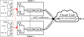
Figure 2: Large-scale MIMO system with C-RAN and AGC.

We initialize the AGC-LRA-MMSE design by computing, for each RRH, the LRA-MMSE receiver that takes into account quantization and a standard AGC as an identity matrix. In order to obtain the optimal AGC coefficients, the derivative of the cost function with respect to the AGC coefficients that takes into account both the presence of an AGC and the LRA-MMSE receive filter is computed in the following. At last, we derive the LRA-MMSE receive filter which works in the CU and considers both the quantization effects and the presence of the AGCs. It is important to mention that no convergence problems were observed in this alternating optimization, which results in accurate symbol estimates. This is quite intuitive since increasingly better estimates $\hat{\mathbf{x}}$ are generated which gives rise to better estimates of the covariance matrices.

III-A Low-Resolution Aware Receive Filter (LRA-MMSE)

The quantized signal vector at $l$-th RRH can be expressed with the help of the Bussgang decomposition [103] as the linear model

$$\begin{split}\mathbf{r}_{l}&=\mathbf{y}_{l}+\mathbf{q}_{l}\\ &=\mathbf{G}_{l}\mathbf{y}_{l}+\mathbf{q}_{l},\end{split}$$ (11)

where $\mathbf{G}_{l}\in\mathbb{R}^{N_{R}\times N_{R}}$ is a diagonal matrix with the real coefficients of the AGC and $\mathbf{q}_{l}\in\mathbb{C}^{N_{R}\times 1}$ is the quantization noise vector. Note that the AGC matrix is assumed to be initialized as an identity matrix. Then, the linear receive filter $\mathbf{W}_{l}\in\mathbb{C}^{KN_{T}\times N_{R}}$ that minimizes the MSE

$$\varepsilon=\mathrm{E}[||\mathbf{x}_{l}-\hat{\mathbf{x}}_{l}||^{2}_{2}]=\mathrm{E}[||\mathbf{x}_{l}-\mathbf{W}_{l}\mathbf{r}_{l}||^{2}_{2}],$$ (12)

is given by

$$\mathbf{W}_{l}=\mathbf{R}_{x_{l}r_{l}}\mathbf{R}_{r_{l}r_{l}}^{-1}.$$ (13)

where the cross-correlation matrix $\mathbf{R}_{x_{l}r_{l}}\in\mathbb{C}^{KN_{T}\times N_{R}}$, and the autocorrelation matrix $\mathbf{R}_{r_{l}r_{l}}\in\mathbb{C}^{N_{R}\times N_{R}}$ are expressed as

$$\mathbf{R}_{x_{l}r_{l}} = \mathbf{R}_{x_{l}y_{l}}+\mathbf{R}_{x_{l}q_{l}},$$ (14)

$$\mathbf{R}_{r_{l}r_{l}} = \mathbf{R}_{y_{l}y_{l}}+\mathbf{R}_{y_{l}q_{l}}+\mathbf{R}_{y_{l}q_{l}}^{H}+\mathbf{R}_{q_{l}q_{l}}.$$ (15)

We obtain the autocorrelation matrix $\mathbf{R}_{y_{l}y_{l}}$ and the cross-correlation matrix $\mathbf{R}_{xy_{l}}$ with the model presented by (4) as

$$\mathbf{R}_{x_{l}y_{l}} = \mathrm{E}[\mathbf{x}_{l}\mathbf{y}_{l}^{H}]=\mathbf{R}_{x_{l}x_{l}}\hat{\mathbf{H}}_{ll}^{H}.$$ (16)

$$\mathbf{R}_{y_{l}y_{l}} = \mathrm{E}[\mathbf{y}_{l}\mathbf{y}_{l}^{H}]=\hat{\mathbf{H}}_{l}\mathbf{R}_{xx}\hat{\mathbf{H}}_{l}^{H}+\mathbf{R}_{n_{l}n_{l}},$$ (17)

To compute (14) and (15) we need to obtain the matrices $\mathbf{R}_{x_{l}q_{l}}$, $\mathbf{R}_{y_{l}q_{l}}$ and $\mathbf{R}_{q_{l}q_{l}}$ as a function of the channel parameters and the distortion factor $\rho_{q}$. Following the procedure developed in [21] the expressions of $\mathbf{R}_{x_{l}q_{l}}$, $\mathbf{R}_{y_{l}q_{l}}$ and $\mathbf{R}_{q_{l}q_{l}}$ are given by

$$\mathbf{R}_{x_{l}q_{l}} = -\rho_{q}\mathbf{R}_{x_{l}y_{l}},$$ (18)

$$\mathbf{R}_{y_{l}q_{l}} \approx -\rho_{q}\mathbf{R}_{y_{l}y_{l}},$$ (19)

$$\mathbf{R}_{q_{l}q_{l}} = \rho_{q}\mathbf{R}_{y_{l}y_{l}}-(1-\rho_{q})\rho_{q}\mathop{\rm nondiag}(\mathbf{R}_{y_{l}y_{l}}).$$ (20)

where nondiag takes its input argument and sets its main diagonal elements to zero, as detailed in the Notation part of the Introduction.

Substituting (16) and (18) in (14), and (17), (19) and (20) in (15) we get

$$\mathbf{R}_{x_{l}r_{l}} \approx (1-\rho_{q})\mathbf{R}_{x_{l}y_{l}}.$$ (21)

$$\mathbf{R}_{r_{l}r_{l}} \approx (1-\rho_{q})(\mathbf{R}_{y_{l}y_{l}}-\rho_{q}\mathop{\rm nondiag}(\mathbf{R}_{y_{l}y_{l}})).$$ (22)

We can then apply (21) and (22) in (13) to obtain the expression of the LRA-MMSE receive filter at the $l$-th RRH

$$\mathbf{W}_{l}\approx\mathbf{R}_{x_{l}y_{l}}(\mathbf{R}_{y_{l}y_{l}}-\rho_{q}\mathop{\rm nondiag}(\mathbf{R}_{y_{l}y_{l}}))^{-1}.$$ (23)

III-B AGC Design

In the following the optimum AGC matrix $\mathbf{G}_{l}$ at the $l$-th RRH is computed by minimizing the MSE. We consider $\mathbf{G}_{l}$ as a diagonal matrix with real coefficients and $\mathbf{g}_{l}$ a vector with the diagonal coefficients of $\mathbf{G}_{l}$. Therefore, we can write $\mathbf{G}_{l}=\mathop{\rm diag}(\mathbf{g}_{l})$. Since $\mathbf{G}_{l}$ is a diagonal matrix with real coefficients we have $\mathop{\rm diag}(\mathbf{g}_{l})^{H}=\mathop{\rm diag}(\mathbf{g}_{l})$. Then, the MSE cost function that considers both the LRA-MMSE receive filter and the AGC matrix at the $l$-th RRH can be rewritten as

$$\varepsilon=\mathrm{E}[||\mathbf{x}_{l}-\mathbf{W}_{l}(\alpha\mathop{\rm diag}(\mathbf{g}_{l})\mathbf{y}_{l}+\mathbf{q}_{l})||^{2}_{2}],$$ (24)

where $\alpha$ corresponds to the clipping factor of the AGC. This factor is a commonly used rule to adjust the amplitude of the received signal in order to minimize the overload distortion [18]. To solve this problem we compute the derivative of (24) with respect to $\mathop{\rm diag}(\mathbf{g}_{l})$ while keeping $\mathbf{W}_{l}$ fixed. Therefore, we will have an initialization using the linear filter previously computed by (23) in order to obtain $\mathbf{G}_{l}$. To compute the optimum $\mathbf{G}_{l}$ matrix we compute the derivative of (24) with respect to $\mathop{\rm diag}(\mathbf{g}_{l})$, equate the derivative terms to zero and solve it for $\mathbf{g}_{l}$:

$$\frac{\partial\varepsilon}{\partial\mathbf{g}_{l}} = -\alpha\underbrace{\frac{\partial\mathop{\rm tr}(\mathbf{R}_{x_{l}y_{l}}\mathop{\rm diag}(\mathbf{g}_{l})\mathbf{W}_{l}^{H})}{\partial\mathbf{g}_{l}}}_{\mathrm{I}}$$ (25)

$$-\alpha\underbrace{\frac{\partial\mathop{\rm tr}(\mathbf{W}_{l}\mathop{\rm diag}(\mathbf{g}_{l})\mathbf{R}_{x_{l}y_{l}}^{H})}{\partial\mathbf{g}_{l}}}_{\mathrm{II}}$$

$$+\alpha^{2}\underbrace{\frac{\partial\mathop{\rm tr}(\mathbf{W}_{l}\mathop{\rm diag}(\mathbf{g}_{l})\mathbf{R}_{y_{l}y_{l}}\mathop{\rm diag}(\mathbf{g}_{l})\mathbf{W}_{l}^{H})}{\partial\mathbf{g}_{l}}}_{\mathrm{III}}$$

$$+\alpha\underbrace{\frac{\partial\mathop{\rm tr}(\mathbf{W}_{l}\mathop{\rm diag}(\mathbf{g}_{l})\mathbf{R}_{y_{l}q_{l}}\mathbf{W}_{l}^{H})}{\partial\mathbf{g}_{l}}}_{\mathrm{IV}}$$

$$+\alpha\underbrace{\frac{\partial\mathop{\rm tr}(\mathbf{W}_{l}\mathbf{R}_{y_{l}q_{l}}^{H}\mathop{\rm diag}(\mathbf{g}_{l})\mathbf{W}_{l}^{H})}{\partial\mathbf{g}_{l}}}_{\mathrm{V}}.$$

The details of the derivation are presented in the Appendix. The results are given by

$$\mathrm{I} =[(\mathbf{R}_{x_{l}y_{l}}^{T}\odot\mathbf{W}_{l}^{H})\mathbf{1}],$$ (26)

$$\mathrm{II} =[(\mathbf{R}_{x_{l}y_{l}}^{H}\odot\mathbf{W}_{l}^{T})\mathbf{1}],$$ (27)

$$\mathrm{III} =[(\mathbf{W}_{l}^{T}\odot(\mathbf{R}_{y_{l}y_{l}}\mathop{\rm diag}(\mathbf{g}_{l})\mathbf{W}_{l}^{H}))\mathbf{1}]$$

$$\hskip 12.0pt+[((\mathbf{R}_{y_{l}y_{l}}^{T}\mathop{\rm diag}(\mathbf{g}_{l})\mathbf{W}_{l}^{T})\odot\mathbf{W}_{l}^{H})\mathbf{1}],$$ (28)

$$\mathrm{IV} =[(\mathbf{W}_{l}^{T}\odot[\mathbf{R}_{y_{l}q_{l}}\mathbf{W}^{H}_{l}])\mathbf{1}],$$ (29)

$$\mathrm{V} =[((\mathbf{R}_{y_{l}q_{l}}^{*}\mathbf{W}_{l}^{T})\odot\mathbf{W}_{l}^{H})\mathbf{1}].$$ (30)

Substituting these results in (25) and solving it for $\mathbf{g}_{l}$ we obtain

$$\mathbf{g}_{l} =[(\mathbf{W}_{l}^{T}\mathbf{W}_{l}^{*})\odot\mathbf{R}_{y_{l}y_{l}}+(\mathbf{W}_{l}^{H}\mathbf{W}_{l})\odot\mathbf{R}_{y_{l}y_{l}}^{T}]^{-1}$$

$$\cdot\frac{2}{\alpha}(\mathrm{Re}([(\mathbf{R}_{x_{l}y_{l}}^{T}\odot\mathbf{W}_{l}^{H})\mathbf{1}])-\mathrm{Re}([(\mathbf{W}_{l}^{T}\odot(\mathbf{R}_{y_{l}q_{l}}\mathbf{W}_{l}^{H}))\mathbf{1}])).$$

In the following we outline the computation of the clipping factor $\alpha$ based on the received signal power. The received signal power at the $l$-th RRH can be computed by

$$P_{l} = \mathop{\rm tr}(\mathbf{R}_{y_{l}y_{l}}+\mathbf{R}_{y_{l}q_{l}}+\mathbf{R}_{y_{l}q_{l}}^{H}+\mathbf{R}_{q_{l}q_{l}}),$$ (31)

and the received symbol energy by

$$E_{rx}=\sqrt{\frac{\mathop{\rm tr}(\mathbf{R}_{y_{l}y_{l}}+\mathbf{R}_{y_{l}q_{l}}+\mathbf{R}_{y_{l}q_{l}}^{H}+\mathbf{R}_{q_{l}q_{l}})}{N_{R}}}.$$ (32)

Thus, the clipping factor $\alpha$ can be obtained from

$$\alpha=\gamma\sqrt{\frac{\mathop{\rm tr}(\mathbf{R}_{y_{l}y_{l}}+\mathbf{R}_{y_{l}q_{l}}+\mathbf{R}_{y_{l}q_{l}}^{H}+\mathbf{R}_{q_{l}q_{l}})}{N_{R}}},$$ (33)

where $\gamma$ is a calibration factor. To ensure an optimized performance, the value of $\gamma$ was set to $\frac{\sqrt{b}}{2}$, which corresponds to the modulus of the last quantizer label.

III-C LRA-MMSE linear receiver in the CU

We assume that the received signals at each RRH are processed by independent AGCs before quantization. After the quantization, both the output signals of the ADCs and the optimized AGC coefficients are sent to the CU. Then, the transmitted signal vector by the $l$-th RRH is expressed by

$$\mathbf{r}_{l}=\mathrm{Q}(\mathrm{diag}(\mathbf{g}_{l})\mathbf{y}_{l})=\mathrm{diag}(\mathbf{g}_{l})\mathbf{y}_{l}+\mathbf{q}_{l}.$$ (34)

In many prior works related to large-scale MIMO and C-RANs, it has been assumed that the receivers are connected to the CU via error-free FH links. However, those assumptions are unrealistic in practical systems. In this work, we assume that the AGC coefficients are sent to the CU through high-resolution control channels of imperfect FH links. Then, those coefficients arrive at the CU with the additive noise due to transmission errors from the FH links. At the CU the received vector with the AGC coefficients from all RRHs of the cluster can be written as

$$\tilde{\mathbf{g}}=\mathbf{g}+\mathbf{n}_{\mathrm{FH}},$$ (35)

where $\mathbf{g}=[\mathbf{g}_{1}^{T},...,\mathbf{g}_{L}^{T}]^{T}$ is the vector with the coefficients of all AGCs of the cluster and $\mathbf{n}_{\mathrm{FH}}\in\mathbb{C}^{LN_{R}\times 1}$ is the vector that models the noise that corrupts the FH transmissions and leads to errors. The elements of $\mathbf{n}_{\mathrm{FH}}$ are considered to be i.i.d ZMCSCG random variables with variance $\sigma_{\tau}^{2}$. From (34) and (35) the digital signal vector at the CU can be expressed as

$$\mathbf{r}_{\mathrm{cu}} = \tilde{\mathbf{G}}(\hat{\mathbf{H}}\mathbf{x}+\mathbf{n})+\mathbf{q}=\tilde{\mathbf{G}}\mathbf{y}+\mathbf{q},$$ (36)

where $\tilde{\mathbf{G}}=\mathop{\rm diag}(\tilde{\mathbf{g}})$, $\mathbf{n}\in\mathbb{C}^{LN_{R}\times 1}$ contains AWGN samples, $\mathbf{q}\in\mathbb{C}^{LN_{R}\times 1}$ is the quantization noise vector, and $\hat{\mathbf{H}}\in\mathbb{C}^{LN_{R}\times LKN_{T}}$ contains the channel coefficients between all users and all RRHs of the cluster. The linear receiver $\mathbf{W}_{LRA}$ that minimizes the MSE cost function

$$\varepsilon=\mathrm{E}[||\mathbf{x}-\hat{\mathbf{x}}||^{2}_{2}]=\mathrm{E}[||\mathbf{x}-\mathbf{W}_{LRA}\mathbf{r}_{\mathrm{cu}}||^{2}_{2}],$$ (37)

is given by

$$\mathbf{W}_{LRA}=\mathbf{R}_{xr_{\mathrm{cu}}}\mathbf{R}_{r_{\mathrm{cu}}r_{\mathrm{cu}}}^{-1},$$ (38)

where the cross-correlation matrix $\mathbf{R}_{xr_{\mathrm{cu}}}\in\mathbb{C}^{LKN_{T}\times LN_{R}}$, and the autocorrelation matrix $\mathbf{R}_{r_{\mathrm{cu}}r_{\mathrm{cu}}}\in\mathbb{C}^{LN_{R}\times LN_{R}}$ are given by

$$\mathbf{R}_{xr_{\mathrm{cu}}} = \mathbf{R}_{xy}\tilde{\mathbf{G}}+\mathbf{R}_{xq},$$

$$\mathbf{R}_{r_{\mathrm{cu}}r_{\mathrm{cu}}} = \tilde{\mathbf{G}}\mathbf{R}_{yy}\tilde{\mathbf{G}}+\tilde{\mathbf{G}}\mathbf{R}_{yq}+\mathbf{R}_{yq}^{H}\tilde{\mathbf{G}}+\mathbf{R}_{qq}.$$

During the detection process, the $i$-th estimated symbol $\hat{x}_{i}$ from the estimated signal vector $\hat{\mathbf{x}}$, is defined as $\mathrm{DEC}(\mathbf{w}_{LRA}(i,:)\mathrm{Q}(\tilde{\mathbf{G}}\mathbf{y}))$, where $\mathrm{DEC}(\cdot)$ is the slicer function appropriate for the modulation scheme being used in the system. From a given constellation alphabet $\mathbb{X}$, this operation chooses the constellation point with smallest Euclidean distance to the estimated symbol,

$$\hat{x}_{i}=\underset{x\in\mathbb{X}}{\mathrm{argmin}}||\mathbf{W}_{LRA}(i,:)\mathrm{Q}(\tilde{\mathbf{G}}\mathbf{y})-x||.$$ (39)

In Algorithm 2 we detail the procedure of how to obtain the AGC of each cell, the LRA-MMSE linear receive filter in the CU and the linear detection scheme.

Algorithm 2 AGC-LRA-MMSE linear receiver

1:Initialize parameters $\rho_{q},\beta,\mathbf{y},\mathbf{R}_{xx},\mathbf{R}_{x_{l}x_{l}},\mathbf{R}_{nn},\mathbf{R}_{n_{l}n_{l}};$

2:for $l=1$ to $L$ do

3:     $\mathbf{R}_{y_{l}y_{l}}=\hat{\mathbf{H}}_{l}\mathbf{R}_{xx}\hat{\mathbf{H}}_{l}^{H}+\mathbf{R}_{n_{l}n_{l}};$

4:     $\mathbf{R}_{x_{l}y_{l}}=\mathbf{R}_{x_{l}x_{l}}\hat{\mathbf{H}}_{ll}^{H};$

5:     $\mathbf{R}_{y_{l}q_{l}}=-\rho_{q}\mathbf{R}_{y_{l}y_{l}};$

6:     $\mathbf{R}_{q_{l}q_{l}}=\rho_{q}\mathbf{R}_{y_{l}y_{l}}-(1-\rho_{q})\rho_{q}\mathop{\rm nondiag}(\mathbf{R}_{y_{l}y_{l}});$

7:     $\mathbf{W}_{l}=\mathbf{R}_{x_{l}y_{l}}(\mathbf{R}_{y_{l}y_{l}}-\rho_{q}\mathop{\rm nondiag}(\mathbf{R}_{y_{l}y_{l}}))^{-1};$

8:     $\alpha=\gamma\cdot\sqrt{\mathop{\rm tr}(\mathbf{R}_{y_{l}y_{l}}+\mathbf{R}_{y_{l}q_{l}}+\mathbf{R}_{y_{l}q_{l}}^{H}+\mathbf{R}_{q_{l}q_{l}})/(N_{R})};$

9:     $\mathbf{g}_{l}=[(\mathbf{W}_{l}^{T}\mathbf{W}_{l}^{*})\odot\mathbf{R}_{y_{l}y_{l}}+(\mathbf{W}_{l}^{H}\mathbf{W}_{l})\odot\mathbf{R}_{y_{l}y_{l}}^{T}]^{-1}\cdot\frac{2}{\alpha}(\mathrm{Re}([(\mathbf{R}_{x_{l}y_{l}}^{T}\odot\mathbf{W}_{l}^{H})\mathbf{1}])-\mathrm{Re}([(\mathbf{W}_{l}^{T}\odot(\mathbf{R}_{y_{l}q_{l}}\mathbf{W}_{l}^{H}))\mathbf{1}]));$

10:end for

11:$\tilde{\mathbf{G}}=\mathop{\rm diag}([\tilde{\mathbf{g}}_{1}^{T},...,\tilde{\mathbf{g}}_{l}^{T},...,\tilde{\mathbf{g}}_{L}^{T}]^{T});$

12:$\mathbf{R}_{yy}=\hat{\mathbf{H}}\mathbf{R}_{xx}\hat{\mathbf{H}}^{H}+\mathbf{R}_{nn};$

13:$\mathbf{R}_{xy}=\mathbf{R}_{xx}\hat{\mathbf{H}}^{H};$

14:$\mathbf{R}_{xq}=-\rho_{q}\mathbf{R}_{xy};$

15:$\mathbf{R}_{yq}=\mathbf{R}_{yy}-(1-\rho_{q})\rho_{q}\mathop{\rm nondiag}(\mathbf{R}_{yy});$

16:$\mathbf{R}_{qq}=\rho_{q}\mathbf{R}_{yy}-(1-\rho_{q})\rho_{q}\mathop{\rm nondiag}(\mathbf{R}_{yy});$

17:$\mathbf{R}_{r_{\mathrm{cu}}r_{\mathrm{cu}}}=\tilde{\mathbf{G}}\mathbf{R}_{yy}\tilde{\mathbf{G}}+\tilde{\mathbf{G}}\mathbf{R}_{yq}+\mathbf{R}_{yq}^{H}\tilde{\mathbf{G}}+\mathbf{R}_{qq};$

18:$\mathbf{R}_{xr_{\mathrm{cu}}}=\mathbf{R}_{xy}\tilde{\mathbf{G}}+\mathbf{R}_{xq};$

19:$\mathbf{W}_{LRA}=\mathbf{R}_{xr_{\mathrm{cu}}}\mathbf{R}_{r_{\mathrm{cu}}r_{\mathrm{cu}}}^{-1};$

20:$\hat{\mathbf{x}}=\mathrm{DEC}(\mathbf{W}_{LRA}\mathrm{Q}(\tilde{\mathbf{G}}\mathbf{y}));$

III-D LRA-MMSE-SIC receiver in the CU

SIC detectors can outperform linear detectors and achieve the sum-capacity in the uplink of multiuser MIMO systems [36]. At each time, a data stream is decoded and its contribution is removed from the received signal. SIC detectors improve the signal-to-interference-plus-noise ratio (SINR) of the remaining symbols that will be detected in the following stages and consequently improve the detection accuracy. Unfortunately, SIC techniques suffer from error propagation. To improve the performance of the SIC detector, in this work data streams are ordered based on channel powers [37, 38].

In the BBU pool the received signal at the $a$-th stage of a SIC detector, $\mathbf{y}^{(a)}\in\mathbb{C}^{LN_{R}\times 1}$, is given by

$$\mathbf{y}^{(a)}=\begin{cases}\mathbf{y}^{(1)},&a=1,\\ \mathbf{y}^{(1)}-\displaystyle\sum_{j=1}^{a-1}\mathbf{h}^{\mathbf{\Phi}(j)}\hat{x}^{\mathbf{\Phi}(j)},&2\leqslant a\leqslant LKN_{T},\end{cases}$$ (40)

where $\hat{x}^{\mathbf{\Phi}(j)}$ is the symbol estimated in the $j$-th stage prior to the $a$-th stage and $\mathbf{h}^{\mathbf{\Phi}(j)}\in\mathbb{C}^{LN_{R}\times 1}$ is the $\mathbf{\Phi}(j)$-th column of $\hat{\mathbf{H}}$. In this notation, $\mathbf{\Phi}$ corresponds to the ordering vector, whose entries indicate what is the symbol that has to be detected at each stage. After detection, the corresponding column $\mathbf{h}^{\mathbf{\Phi}(a)}$ from the channel matrix $\hat{\mathbf{H}}^{(a)}\in\mathbb{C}^{LN_{R}\times(LKN_{T}-a+1)}$ is cancelled and another LRA-MMSE receive filter is computed for the next stage. The quantized received signal vector $\mathbf{r}^{(a)}\in\mathbb{C}^{LN_{R}\times 1}$ at the $a$-th stage is given by

$$\mathbf{r}^{(a)}_{\mathrm{cu}}=\mbox{Q}(\tilde{\mathbf{G}}\mathbf{y}^{(a)})=\tilde{\mathbf{G}}(\hat{\mathbf{H}}^{(a)}\mathbf{x}^{(a)}+\mathbf{n})+\mathbf{q}^{(a)}.$$ (41)

The LRA-MMSE linear receive filter of the SIC detector is given by

$$\mathbf{W}_{LRA}^{(a)}=\mathbf{R}_{xr_{\mathrm{CU}}}^{(a)}(\mathbf{R}_{r_{\mathrm{CU}}r_{\mathrm{CU}}}^{(a)})^{-1},$$ (42)

where the cross-correlation matrix $\mathbf{R}_{xr}^{(a)}\in\mathbb{C}^{(LKN_{T}-a+1)\times LN_{R}}$ and the autocorrelation matrix $\mathbf{R}_{rr}^{(a)}\in\mathbb{C}^{LN_{R}\times LN_{R}}$ are given by

$$\mathbf{R}_{xr_{\mathrm{CU}}}^{(a)} = \mathbf{R}_{xy}^{(a)}\tilde{\mathbf{G}}+\mathbf{R}_{xq}^{(a)},$$ (43)

$$\mathbf{R}_{r_{\mathrm{CU}}r_{\mathrm{CU}}}^{(a)} = \tilde{\mathbf{G}}\mathbf{R}_{yy}^{(a)}\tilde{\mathbf{G}}+\tilde{\mathbf{G}}\mathbf{R}_{yq}^{(a)}+(\mathbf{R}_{yq}^{(a)})^{H}\tilde{\mathbf{G}}$$ (44)

$$+\mathbf{R}_{qq}^{(a)}.$$

The joint AGC and LRA-MMSE linear receive filter design with SIC detection scheme is illustrated in Algorithm 3.

Algorithm 3 AGC-LRA-MMSE with SIC receiver

1:Initialize parameters $\rho_{q},\beta,\mathbf{y},\mathbf{R}_{xx},\mathbf{R}_{x_{l}x_{l}},\mathbf{R}_{nn},\mathbf{R}_{n_{l}n_{l}};$

2:Ordering $\mathbf{\Phi}=[\Phi_{1},\Phi_{2},...,\Phi_{LKN_{T}}];$

3:for $l=1$ to $L$ do

4:     $\mathbf{R}_{y_{l}y_{l}}=\hat{\mathbf{H}}_{l}\mathbf{R}_{xx}\hat{\mathbf{H}}_{l}^{H}+\mathbf{R}_{n_{l}n_{l}};$

5:     $\mathbf{R}_{x_{l}y_{l}}=\mathbf{R}_{x_{l}x_{l}}\hat{\mathbf{H}}_{ll}^{H};$

6:     $\mathbf{R}_{y_{l}q_{l}}=-\rho_{q}\mathbf{R}_{y_{l}y_{l}};$

7:     $\mathbf{R}_{q_{l}q_{l}}=\rho_{q}\mathbf{R}_{y_{l}y_{l}}-(1-\rho_{q})\rho_{q}\mathop{\rm nondiag}(\mathbf{R}_{y_{l}y_{l}});$

8:     $\mathbf{W}_{l}=\mathbf{R}_{x_{l}y_{l}}(\mathbf{R}_{y_{l}y_{l}}-\rho_{q}\mathop{\rm nondiag}(\mathbf{R}_{y_{l}y_{l}}))^{-1};$

9:     $\alpha=\gamma\cdot\sqrt{\mathop{\rm tr}(\mathbf{R}_{y_{l}y_{l}}+\mathbf{R}_{y_{l}q_{l}}+\mathbf{R}_{y_{l}q_{l}}^{H}+\mathbf{R}_{q_{l}q_{l}})/(N_{R})};$

10:     $\mathbf{g}_{l}=[(\mathbf{W}_{l}^{T}\mathbf{W}_{l}^{*})\odot\mathbf{R}_{y_{l}y_{l}}+(\mathbf{W}_{l}^{H}\mathbf{W}_{l})\odot\mathbf{R}_{y_{l}y_{l}}^{T}]^{-1}\cdot\frac{2}{\alpha}(Re([(\mathbf{R}_{x_{l}y_{l}}^{T}\odot\mathbf{W}_{l}^{H})\mathbf{1}])-Re([(\mathbf{W}_{l}^{T}\odot(\mathbf{R}_{y_{l}q_{l}}\mathbf{W}_{l}^{H}))\mathbf{1}]));$

11:end for

12:$\tilde{\mathbf{G}}=\mathop{\rm diag}([\tilde{\mathbf{g}}_{1}^{T},...,\tilde{\mathbf{g}}_{l}^{T},...,\tilde{\mathbf{g}}_{L}^{T}]^{T});$

13:for $a=1$ to $LKN_{T}$ do

14:     $\mathbf{R}_{yy}=\hat{\mathbf{H}}\mathbf{R}_{xx}\hat{\mathbf{H}}^{H}+\mathbf{R}_{nn};$

15:     $\mathbf{R}_{xy}=\mathbf{R}_{xx}\hat{\mathbf{H}}^{H};$

16:     $\mathbf{R}_{xq}=-\rho_{q}\mathbf{R}_{xy};$

17:     $\mathbf{R}_{yq}=\mathbf{R}_{yy}-(1-\rho_{q})\rho_{q}\mathop{\rm nondiag}(\mathbf{R}_{yy});$

18:     $\mathbf{R}_{qq}=\rho_{q}\mathbf{R}_{yy}-(1-\rho_{q})\rho_{q}\mathop{\rm nondiag}(\mathbf{R}_{yy});$

19:     $\mathbf{R}_{r_{\mathrm{cu}}r_{\mathrm{cu}}}=\tilde{\mathbf{G}}\mathbf{R}_{yy}\tilde{\mathbf{G}}+\tilde{\mathbf{G}}\mathbf{R}_{yq}+\mathbf{R}_{yq}^{H}\tilde{\mathbf{G}}+\mathbf{R}_{qq};$

20:     $\mathbf{R}_{xr_{\mathrm{cu}}}=\mathbf{R}_{xy}\tilde{\mathbf{G}}+\mathbf{R}_{xq};$

21:     $\mathbf{W}_{LRA}=\mathbf{R}_{xr_{\mathrm{cu}}}\mathbf{R}_{r_{\mathrm{cu}}r_{\mathrm{cu}}}^{-1};$

22:     $\hat{x}=\mathrm{DEC}(\mathbf{W}_{LRA}(\mathbf{\Phi}(a),:)\mbox{Q}(\tilde{\mathbf{G}}\mathbf{y}));$

23:     $\mathbf{y}=\mathbf{y}-\mathbf{H}(:,\mathbf{\Phi}(a))\hat{x};$

24:     $\mathbf{H}(:,\mathbf{\Phi}(a))=\mathop{\rm zeros}(LN_{R},1);$

25:end for

III-E Computational Complexity

The computational complexity of the proposed AGC-LRA-MMSE linear and SIC receivers can be exactly computed as a function of the number of receive and transmit antennas, the number of users per cell and the number of cells as depicted in Table I. To assess the computational complexity of the AGC-LRA-MMSE receivers we have computed the number of arithmetic operations such as complex additions and multiplications.

To initialize the AGC-LRA-MMSE algorithm, a linear receive filter $\mathbf{W}_{l}$ is computed for each cell by (23). The largest contribution in terms of computational complexity in the computation of $\mathbf{W}_{l}$ is due to the inversion of $\mathbf{R}_{r_{l}r_{l}}\in\mathbb{C}^{N_{R}\times N_{R}}$. In this work we consider that the inversion of an $N\times N$ matrix by Gaussian elimination costs $\mathop{\mathcal{O}}(N^{3})$ operations. Therefore, the computational cost to obtain each $\mathbf{W}_{l}$ matrix is $\mathop{\mathcal{O}}(N_{R}^{3})$. After that, an AGC matrix $\mathop{\rm diag}(\mathbf{g}_{l})$ with a computational cost of $\mathop{\mathcal{O}}(N_{R}^{3})$ is computed for each RRH. Then, an LRA linear receive filter $\mathbf{W}_{LRA}$ is computed by (38), which requires the inversion of the matrix $\mathbf{R}_{rr}\in\mathbb{C}^{LN_{R}\times LN_{R}}$. Thus, the computational complexity to obtain $\mathbf{W}_{LRA}$ is $\mathop{\mathcal{O}}(L^{3}N_{R}^{3})$. Summarizing these results, the proposed AGC-LRA-MMSE linear receive filter has a total cost of $\mathop{\mathcal{O}}\left(N_{R}^{3}(L^{3}+2L)\right)$. When we employ SIC detection with the AGC-LRA-MMSE receiver filter an $W_{LRA}^{(a)}$ matrix is computed to detect a symbol at each stage of the interference cancellation. Thus, as we consider the transmission of $LKN_{T}$ streams, the expression of the LRA-MMSE receive filter $W_{LRA}^{(a)}$ is computed $LKN_{T}$ times to detect all data streams. Therefore, the computational complexity of the proposed AGC-LRA-MMSE-SIC algorithm is $\mathop{\mathcal{O}}\left(L^{4}N_{R}^{3}KN_{T}\right)$. We remark that these costs can be reduced by the efficient use signal processing algorithms, which can be investigated in a future work.

TABLE I: Computational complexity of algorithms.

Task	Additions	Multiplications
FR Standard MMSE	$\mathop{\mathcal{O}}(L^{3}N_{R}^{3})$	$\mathop{\mathcal{O}}(L^{3}N_{R}^{3})$
AGC-LRA-MMSE	$\mathop{\mathcal{O}}\left(N_{R}^{3}(L^{3}+2L)\right)$	$\mathop{\mathcal{O}}\left(N_{R}^{3}(L^{3}+2L)\right)$
AGC-LRA-MMSE-SIC	$\mathop{\mathcal{O}}\left(L^{4}N_{R}^{3}KN_{T}\right)$	$\mathop{\mathcal{O}}\left(L^{4}N_{R}^{3}KN_{T}\right)$

IV Sum rate analysis

In this section, assuming Gaussian signaling, we derive expressions for the achievable sum rates of the proposed joint AGC and LRA-MMSE receive filter design in large-scale MIMO with C-RAN systems for linear and SIC schemes.

IV-A Sum Rate of Linear Receivers

The ergodic sum rate $\mathcal{R}_{\mathop{\rm sum}}$ of the system with the AGC-LRA-MMSE linear receive filter is given by the sum of the achievable rates of each user in the cluster, averaged over the channel realizations as described by

$$\mathcal{R}_{\mathop{\rm sum}} =\sum_{l=1}^{L}\sum_{k=1}^{K}\mathrm{E}_{\mathbf{H}}[\mathcal{R}_{l}^{(k)}].$$ (45)

The achievable rate $\mathcal{R}_{l}^{(k)}$ of the $k$-th user in the $l$-th cell is calculated as

$$\mathcal{R}_{l}^{(k)}=\log_{2}\det(\mathbf{I}_{N_{T}}+\Lambda_{l}^{(k)}),$$ (46)

where $\Lambda_{l}^{(k)}$ denotes a matrix associated with the post processing signal-to-interference-plus-noise ratio (SINR) of the $k$-th user in the $l$-th cell given by

$$\Lambda_{l}^{(k)}=\mathbf{\Upsilon}_{l}^{(k)}(\mathbf{\Gamma}_{l}^{(k)})^{-1},$$ (47)

where $\mathbf{\Upsilon}_{l}^{(k)}$ represents the covariance matrix of the desired signal and $\mathbf{\Gamma}_{l}^{(k)}$ represents the covariance matrix of the noise plus interference [20, 104, 105]. At the BBU pool, the received signals of the cluster can be computed by (36). Assuming that the BBU pool employs the LRA-MMSE receiver to detect the symbols transmitted by the users, we can compute the estimated symbol of the $k$-th user at the $l$-th cell by

$$\hat{\mathbf{x}}_{l}^{(k)} =\mathbf{W}_{LRA,l}^{(k)}\tilde{\mathbf{G}}\hat{\mathbf{H}}_{l}^{(k)}\mathbf{x}_{l}^{(k)}+\sum_{\stackrel{{\scriptstyle u=1}}{{u\neq k}}}^{K}\mathbf{W}_{LRA,l}^{(k)}\tilde{\mathbf{G}}\hat{\mathbf{H}}_{l}^{(u)}\mathbf{x}_{l}^{(u)}$$

$$+\sum_{\stackrel{{\scriptstyle j=1}}{{j\neq l}}}^{L}\sum_{u=1}^{K}\mathbf{W}_{LRA,l}^{(k)}\tilde{\mathbf{G}}\hat{\mathbf{H}}_{j}^{(u)}\mathbf{x}_{j}^{(u)}+\mathbf{W}_{LRA,l}^{(k)}\tilde{\mathbf{G}}\mathbf{n}$$

$$+\mathbf{W}_{LRA,l}^{(k)}\mathbf{q}.$$ (48)

In (48), the first term corresponds to the estimation of the desired symbol and the other terms are interferences. Thus, the covariance matrix of the desired signal is given by

$$\mathbf{\Upsilon}_{l}^{(k)}=\sigma_{x}^{2}(\mathbf{W}_{LRA,l}^{(k)}\tilde{\mathbf{G}}\hat{\mathbf{H}}_{l}^{(k)})(\mathbf{W}_{LRA,l}^{(k)}\tilde{\mathbf{G}}\hat{\mathbf{H}}_{l}^{(k)})^{H}.$$ (49)

The other terms of (48) are the interferences present in the system such as the intracell interference, the intercell interference, the AWGN and the quantization distortion. Therefore, the covariance matrix of the noise plus interference part can be obtained by

$$\mathbf{\Gamma}_{l}^{(k)}= \sigma_{x}^{2}\sum_{\stackrel{{\scriptstyle u=1}}{{u\neq k}}}^{K}(\mathbf{W}_{LRA,l}^{(k)}\tilde{\mathbf{G}}\hat{\mathbf{H}}_{l}^{(u)})(\mathbf{W}_{LRA,l}^{(k)}\tilde{\mathbf{G}}\hat{\mathbf{H}}_{l}^{(u)})^{H}$$

$$-\rho_{q}\sigma_{x}^{2}\sum_{\stackrel{{\scriptstyle u=1}}{{u\neq k}}}^{K}(\mathbf{W}_{LRA,l}^{(k)}\hat{\mathbf{H}}_{l}^{(u)})(\mathbf{W}_{LRA,l}^{(k)}\tilde{\mathbf{G}}\hat{\mathbf{H}}_{l}^{(u)})^{H}$$

$$-\rho_{q}\sigma_{x}^{2}\sum_{\stackrel{{\scriptstyle u=1}}{{u\neq k}}}^{K}(\mathbf{W}_{LRA,l}^{(k)}\tilde{\mathbf{G}}\hat{\mathbf{H}}_{l}^{(u)})(\mathbf{W}_{LRA,l}^{(k)}\hat{\mathbf{H}}_{l}^{(u)})^{H}$$

$$+\sigma_{x}^{2}\sum_{\stackrel{{\scriptstyle j=1}}{{i\neq l}}}^{L}\sum_{u=1}^{K}(\mathbf{W}_{LRA,l}^{(k)}\tilde{\mathbf{G}}\hat{\mathbf{H}}_{j}^{(u)})(\mathbf{W}_{LRA,l}^{(k)}\tilde{\mathbf{G}}\hat{\mathbf{H}}_{j}^{(u)})^{H}$$

$$-\rho_{q}\sigma_{x}^{2}\sum_{\stackrel{{\scriptstyle i=1}}{{i\neq l}}}^{L}\sum_{u=1}^{K}(\mathbf{W}_{LRA,l}^{(k)}\hat{\mathbf{H}}_{j}^{(u)})(\mathbf{W}_{LRA,l}^{(k)}\tilde{\mathbf{G}}\hat{\mathbf{H}}_{j}^{(u)})^{H}$$

$$-\rho_{q}\sigma_{x}^{2}\sum_{\stackrel{{\scriptstyle i=1}}{{i\neq l}}}^{L}\sum_{u=1}^{K}(\mathbf{W}_{LRA,l}^{(k)}\tilde{\mathbf{G}}\hat{\mathbf{H}}_{j}^{(u)})(\mathbf{W}_{LRA,l}^{(k)}\hat{\mathbf{H}}_{j}^{(u)})^{H}$$

$$+\sigma_{n}^{2}(\mathbf{W}_{LRA,l}^{(k)}\tilde{\mathbf{G}})(\mathbf{W}_{LRA,l}^{(k)}\tilde{\mathbf{G}})^{H}$$

$$-\rho_{q}\sigma_{n}^{2}(\mathbf{W}_{LRA,l}^{(k)})(\mathbf{W}_{LRA,l}^{(k)}\tilde{\mathbf{G}})^{H}$$

$$-\rho_{q}\sigma_{n}^{2}(\mathbf{W}_{LRA,l}^{(k)}\tilde{\mathbf{G}})(\mathbf{W}_{LRA,l}^{(k)})^{H}+\mathbf{W}_{LRA,l}^{(k)}\rho_{q}\cdot$$

$$(\mathbf{R}_{yy}-(1-\rho_{q})\mathop{\rm nondiag}(\mathbf{R}_{yy}))\mathbf{W}_{LRA,l}^{(k)H}.$$ (50)

Substituting (49) and (50) in (47) we get the expression of the matrix associated with the post processing SINR of the $k$-th user in the $l$-th cell. Then, we can substitute (47) in (46) to get the achievable rate $\mathcal{R}_{l}^{(k)}$. Using (46) the ergodic sum rate $\mathcal{R}_{\mathop{\rm sum}}$ of the system, averaged over channel realizations, is described by

$$\mathcal{R}_{\mathop{\rm sum}}=\sum_{l=1}^{L}\sum_{k=1}^{K}\mathrm{E}_{\mathbf{H}}[\log_{2}\det(\mathbf{I}_{N_{T}}+\mathbf{\Upsilon}_{l}^{(k)}(\mathbf{\Gamma}_{l}^{(k)})^{-1})].$$ (51)

IV-B Sum Rate of SIC receivers

The uplink sum rate of the SIC receivers based on the proposed AGC-LRA-MMSE design in a system with $LKN_{T}$ interfering layers can be computed by the sum of the achievable rate of the $a$-th stream after the linear receiver with the AGC-LRA-MMSE design, and the achievable rate of the reduced size $(LKN_{T}-a)\times LN_{R}$ MIMO system after removal of the $a$-th stream, given by

$$\mathcal{R}_{\mathop{\rm sum}}=\sum_{a=1}^{MKN_{T}}\mathrm{E}_{\mathbf{H}}\left[\log_{2}\left(1+\frac{\Upsilon^{\mathbf{\Phi}(a)}}{\Gamma^{\mathbf{\Phi}(a)}}\right)\right],$$ (52)

where $\Upsilon^{\mathbf{\Phi}(a)}$ is the desired signal power and $\Gamma^{\mathbf{\Phi}(a)}$ is the interference-plus-noise power. The expectation is taken over the channel coefficients. In the $a$-th stage, the estimated symbol is given by

$$\hat{x}_{l}^{\mathbf{\Phi}(a)}= \mathbf{w}_{LRA,l}^{\mathbf{\Phi}(a)}\tilde{\mathbf{G}}\hat{\mathbf{h}}_{l}^{\mathbf{\Phi}(a)}x_{l}^{\mathbf{\Phi}(a)}+\sum_{\stackrel{{\scriptstyle u=1}}{{u\neq\mathbf{\Phi}(a)}}}^{KN_{T}}\mathbf{w}_{LRA,l}^{\mathbf{\Phi}(a)}\tilde{\mathbf{G}}\hat{\mathbf{h}}_{l}^{(u)}x_{l}^{(u)}$$

$$+\sum_{\stackrel{{\scriptstyle j=1}}{{j\neq l}}}^{L}\sum_{u=1}^{KN_{T}}\mathbf{w}_{LRA,l}^{\mathbf{\Phi}(a)}\tilde{\mathbf{G}}\hat{\mathbf{h}}_{j}^{(u)}x_{j}^{(u)}+\mathbf{w}_{LRA,l}^{\mathbf{\Phi}(a)}\tilde{\mathbf{G}}\mathbf{n}$$

$$+\mathbf{w}_{LRA,l}^{\mathbf{\Phi}(a)}\mathbf{q},\hskip 15.0pt\{x_{l}^{\mathbf{\Phi}(a)},x_{l}^{(u)},x_{j}^{(u)}\}\not\subset\mathbf{\Omega},$$ (53)

where $\mathbf{\Omega}$ is a set of symbols estimated at prior stages. The coefficients of the receive filter $\mathbf{w}_{LRA,l}^{\mathbf{\Phi}(a)}$ are obtained from the $\mathbf{\Phi}(a)$-th row of the filter matrix $\mathbf{W}_{LRA}^{(a)}$. Given a channel realization $\hat{\mathbf{H}}$, the desired signal power is computed by

$$\Upsilon^{\mathbf{\Phi}(a)}=\sigma_{x}^{2}(\mathbf{w}_{LRA,l}^{\mathbf{\Phi}(a)}\tilde{\mathbf{G}}\hat{\mathbf{h}}_{l}^{\mathbf{\Phi}(a)})(\mathbf{w}_{LRA,l}^{\mathbf{\Phi}(a)}\tilde{\mathbf{G}}\hat{\mathbf{h}}_{l}^{\mathbf{\Phi}(a)})^{H},$$ (54)

where $\hat{\mathbf{h}}^{\mathbf{\Phi}(j)}_{l}$ is the $\mathbf{\Phi}(j)$-th column of $\hat{\mathbf{H}}^{(a)}$. Then, $\hat{\mathbf{h}}_{l}^{\mathbf{\Phi}(a)}$ becomes null and the interference-plus-noise power is given by

$$\Gamma^{\mathbf{\Phi}(a)}= \sigma_{x}^{2}(\mathbf{w}_{LRA,l}^{\mathbf{\Phi}(a)}\tilde{\mathbf{G}}\hat{\mathbf{H}}^{(a)})(\mathbf{w}_{LRA,l}^{\mathbf{\Phi}(a)}\tilde{\mathbf{G}}\hat{\mathbf{H}}^{(a)})^{H}$$

$$-\rho_{q}\sigma_{x}^{2}[(\mathbf{w}_{LRA,l}^{\mathbf{\Phi}(a)}\hat{\mathbf{H}}_{l}^{(a)})(\mathbf{w}_{LRA,l}^{\mathbf{\Phi}(a)}\tilde{\mathbf{G}}\hat{\mathbf{H}}_{l}^{(a)})^{H}$$

$$+(\mathbf{w}_{LRA,l}^{\mathbf{\Phi}(a)}\tilde{\mathbf{G}}\hat{\mathbf{H}}_{l}^{(a)})(\mathbf{w}_{LRA,l}^{\mathbf{\Phi}(a)}\hat{\mathbf{H}}_{l}^{(a)})^{H}$$

$$+\sum_{\stackrel{{\scriptstyle j=1}}{{j\neq l}}}^{L}(\mathbf{w}_{LRA,l}^{\mathbf{\Phi}(a)}\hat{\mathbf{H}}_{j}^{(a)})(\mathbf{w}_{LRA,l}^{\mathbf{\Phi}(a)}\tilde{\mathbf{G}}\hat{\mathbf{H}}_{j}^{(a)})^{H}$$

$$+\sum_{\stackrel{{\scriptstyle j=1}}{{j\neq l}}}^{L}(\mathbf{w}_{LRA,l}^{\mathbf{\Phi}(a)}\tilde{\mathbf{G}}\hat{\mathbf{H}}_{j}^{(a)})(\mathbf{w}_{LRA,l}^{\mathbf{\Phi}(a)}\hat{\mathbf{H}}_{j}^{(a)})^{H}]$$

$$+\sigma_{n}^{2}(\mathbf{w}_{LRA,l}^{\mathbf{\Phi}(a)}\tilde{\mathbf{G}})(\mathbf{w}_{LRA,l}^{\mathbf{\Phi}(a)}\tilde{\mathbf{G}})^{H}$$

$$-\rho_{q}\sigma_{n}^{2}[(\mathbf{w}_{LRA,l}^{\mathbf{\Phi}(a)})(\mathbf{w}_{LRA,l}^{\mathbf{\Phi}(a)}\tilde{\mathbf{G}})^{H}$$

$$+(\mathbf{w}_{LRA,l}^{\mathbf{\Phi}(a)}\tilde{\mathbf{G}})(\mathbf{w}_{LRA,l}^{\mathbf{\Phi}(a)})^{H}]+\mathbf{w}_{LRA}^{\mathbf{\Phi}(a)}\rho_{q}\cdot$$

$$(\mathbf{R}_{yy}-(1-\rho_{q})\mathop{\rm nondiag}(\mathbf{R}_{yy}))\mathbf{w}_{LRA}^{\mathbf{\Phi}(a)H},$$ (55)

where $\hat{\mathbf{H}}_{l}^{(a)}$ is the channel matrix between the users in the $l$-th cell and all receive antennas of the cluster. Substituting (54) and (55) in (52) we get the achievable sum rate $\mathcal{R}_{\mathop{\rm sum}}$ of the system when SIC receivers with the proposed AGC-LRA-MMSE design are employed. Since the channels are assummed to be wide-sense stationary and drawn from ergodic processes, then $\mathrm{E}_{\mathbf{H}}$ may be replaced by a simple average over $LH$ in (46) and an average over $MKN_{T}$ in (52). As one may realize from (46) and (52), the higher the SINR of the system, the higher is the sum rate for both linear and SIC designs.

V Simulation Results

In this section, we discuss the BER performance and the achievable sum rate associated with the proposed algorithms and compare them with the existing techniques in a large-scale MU-MIMO system where the received signals are detected in C-RANs. For our simulations, we consider the uplink channel of a large-scale MU-MIMO system comprised by one cluster with 4 cells. Each cell contains one centralized RRH equipped with $N_{R}=64$ receive antennas and $K=8$ users, equipped with $N_{T}=2$ transmit antennas each. The users are distributed randomly and uniformly over the covered area. Moreover, it is also considered that the RRHs share the same frequency band and the system is perfectly synchronized. Synchronization problems can be considered in an even more real scenario. However, a study of the impact of synchronization is not the goal of this work and thus it is left to a future work. The following results show the performance achieved by using both linear and SIC detection schemes.

The channel model used in the simulations includes fast fading, geometric attenuation, and log-normal shadow fading. The small-scale fading is modeled by a Rayleigh channel whose coefficients are i.i.d complex Gaussian random variables with zero-mean and unit variance. The large-scale fading coefficients are obtained by (2), where the path-loss exponent is $\gamma=3.7$, and the shadow-fading standard deviation is $\sigma_{\mathrm{shadow}}=8.0$ dB. We consider a cell radius of one kilometer and the users are distributed in a covered area between a cell-hole radius of 10 meters and the cell edge. For each channel realization, each transmit antenna of each user transmits data packets with $100$ symbols using either quadrature phase-shift keying (QPSK) or 16-ary quadrature amplitude modulation (16-QAM). The results are generated using MATLAB and taking the average of $10^{3}$ channels for both the sum rate and the BER plots. In addition, for each channel realization we have considered $10^{5}$ symbol vectors and checked if the number of errors was at least $100$ such that the computation of BER curves is sufficiently accurate.. In each RRH the received signals are treated by independent AGCs and then quantized by uniform quantizers with $b$-bits of resolution before being sent to the CU. In the presented results, the receivers that employ SIC detection scheme are ordered by the channel norms.

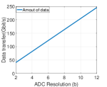
(a) Data transfer.

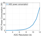
(b) Power consumption.

Figure 3: Amount of required data transfer and total ADC power consumption.

To highlight how important it is the reduction of the resolution of the ADCs and the achieved gains of the proposed design we illustrate the amount of data that have to be transported through the FH links and the power consumption by the quantization step of the considered scenario. In this paper, we consider that the system bandwidth is equal to $B=20$ MHz. To avoid aliasing we adopt a sampling rate of $W=2B$ in order to satisfy the Nyquist theorem [18]. The relation between the required data transfer through the FH links and the ADC resolution can be computed as $T(b)=2MN_{R}Wb$, which is illustrated in Fig. 3a. The power consumption of each ADC can be calculated as $P_{\mbox{ADC}}(b)=cW2^{b}$, where $c$ is the power consumption per conversion step (conv-step). This power consumption model of the ADC encompasses various architectures and implementations of ADCs which are described in [107, 106, 108]. Considering an energy consumption per conversion step $c=494$ fJ [107, 108], the total power consumption by the ADCs is given by $P(b)=2MN_{R}cW2^{b}$, which is illustrated, with the proposed example parameters, in Fig. 3b. The curves of Fig. 3 shows that the deployment of low-resolution techniques can substantially reduce the power consumption from existing solutions that employ high-resolution ADCs (namely 8-12 bits). In particular, the saving in power consumption due to the ADCs in greater than $90\%$. Moreover, the saving in data transfer due the reduction in the number of bits transmitted over the FH links is also significant.

In Fig. 4 we investigate the advantages of the proposed AGC-LRA-MMSE receiver design with SIC detection scheme (AGC-LRA-MMSE-SIC) in terms of BER performance when users transmit QPSK symbols. Here we consider that the CSIR is perfectly known and there are not errors in the transmission of the AGC coefficients over the FH links. To investigate the performance gain we consider the Modified MMSE receiver presented in [23] and the standard AGC from [24] with the standard MMSE receiver. For a fair comparison we also employ [23] with the SIC detection scheme. The results reveal that, for signals quantized with $6$ bits, the proposed AGC-LRA-MMSE-SIC approach achieves a very close performance to the performance achieved by the Full-Resolution (FR) Standard MMSE-SIC receiver in a system with unquantized signals. Moreover, the proposed AGC-LRA-MMSE-SIC detection scheme has a significantly better performance than existing techniques.

By increasing the modulation order we consider in Fig. 5 users transmitting 16-QAM modulation symbols. A comparison of Fig. 5 and Fig. 4 shows a significant performance loss due to the higher modulation order. This is expected because the constellation points of the 16-QAM modulation scheme are closer to each other than the constellation points of the QPSK modulation scheme. Thus, the detection of symbols of a higher modulation order is more sensitive to interference. Despite that, Fig. 5 shows a very small gap between the BER achieved by the FR Standard MMSE-SIC scheme and by the proposed AGC-LRA-MMSE-SIC scheme when signals are quantized with $5$ or $6$ bits. Furthermore, we can notice the poor performance achieved by existing techniques when a higher modulation order is considered. The analysis of this result reveals that the proposed AGC-LRA-MMSE-SIC scheme can improve the BER performance even when users transmit symbols of a higher modulation order.

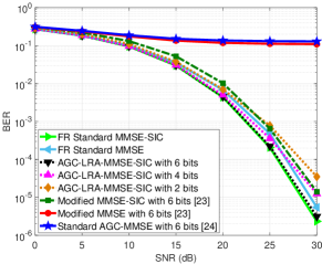
Figure 4: Uncoded BER performance comparison with QPSK modulation considering perfect CSIR.

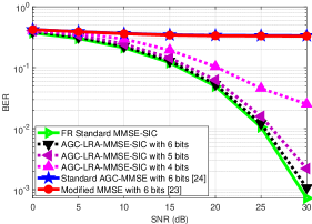
Figure 5: Uncoded BER performance comparison with 16-QAM modulation.

Next we investigate the influence of the imperfect FH links by the possible transmission errors when the optimal AGC coefficients arrive at the CU. In Fig. 6 we consider the same setting as in Fig. 4, but now we take into account the FH transmission errors model as presented by (35). This result shows that even in the presence of errors in the AGC coefficients, the proposed scheme achieves a BER performance close to the FR Standard MMSE-SIC receiver and achieves a better performance than existing techniques.

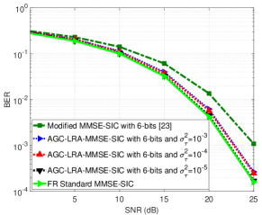
Figure 6: AGC-LRA-MMSE-SIC receiver uncoded BER performance comparison with QPSK modulation considering perfect CSIR and $\sigma_{\tau}^{2}\in\{10^{-3},10^{-4},10^{-5}\}$.

In order to investigate the BER performance of the proposed AGC-LRA-MMSE-SIC receiver in a system without perfect CSIR we consider the imperfect CSI model described by (3). Fig. 7 illustrates the BER performance achieved by the receiver algorithms in a scenario with the CSI related parameter $\eta\in\{0.1,0.25,0.5\}$. This result shows the close performance achieved by the AGC-LRA-MMSE-SIC receiver in a scenario whose signals are quantized with 6 bits, and with imperfect CSI, to the performance achieved by the FR-MMSE-SIC receiver with unquantized signals and with perfect CSI. This result confirms that there are no convergence problems in the proposed joint optimization of the AGC and the LRA-MMSE receiver design when the channel is imperfectly known. Moreover, the proposed AGC-LRA-MMSE-SIC receiver still has a better performance than existing techniques even with channel estimation errors.

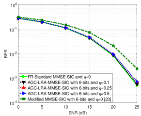
Figure 7: AGC-LRA-MMSE-SIC receiver uncoded BER performance comparison with QPSK modulation considering imperfect CSIR with $\eta\in\{0.1,0.25,0.5\}$.

In the following results we investigate the sum rates achieved by the proposed AGC-LRA-MMSE receiver by using both linear and SIC detection schemes. Fig. 8 compares the achievable sum rates by the AGC-LRA-MMSE linear receiver and the sum rates achieved by the FR Standard MMSE receiver. In this result is possible to see that, the proposed AGC-LRA-MMSE linear receiver achieves a sum rate similar to the sum rate achieved by the FR Standard MMSE receiver, even in a system whose signals are quantized with only $6$ or $5$ bits.

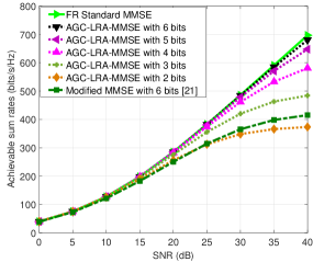
Figure 8: Achievable sum rates of the proposed AGC-LRA-MMSE linear scheme.

In Fig. 9 we investigate achievable sum rates when the proposed AGC-LRA-MMSE receiver is employed with SIC detection scheme. As expected, the AGC-LRA-MMSE-SIC scheme achieves a higher sum rate than that of the linear AGC-LRA-MMSE receiver due to the SIC detection technique that improves the SINR of each stream by the interference removal of the streams already detected. Similarly to the linear case, the sum rates achieved by the AGC-LRA-MMSE-SIC scheme in a system whose signals are quantized with $5$ bits is close to the sum rates achieved by the FR Standard MMSE-SIC receiver with unquantized signals.

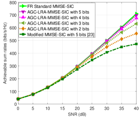
Figure 9: Achievable sum rates of the proposed AGC-LRA-MMSE-SIC scheme.

VI Conclusions

In this paper we have proposed the AGC-LRA-MMSE receiver design that jointly optimizes the AGCs that work in the RRHs and the receive filters that work in the CU for large-scale MU-MIMO systems in C-RANs with low-resolution quantized signals. The optimized AGC adjusts the dynamic range of the input signals inside the range of the quantizer in order to reduce the overload and the granular distortions. Their coefficients are calculated taking into account both the presence of the receive filter and the impact of quantization, which implies in a more accurate AGC than existing techniques. The proposed design has been incorporated into SIC detection scheme, resulting in substantial performance advantages over existing approaches. In particular, for QPSK modulation the AGC-LRA-MMSE-SIC design can save up to $3$ dB in SNR in comparison to the best known approach [23] for the same BER performance, whereas the gains in achievable sum rate are up to about $45\%$ over the best known approach [23]. Furthermore, the sum rates and the BER achieved are very close to those of unquantized systems for signals quantized with $5$ or $6$ bits. Therefore, the proposed AGC-LRA-MMSE-SIC design allows the use of low-resolution ADCs in large scale MU-MIMO systems with C-RANs that are important to improve the energy efficiency of wireless systems and to compress signals, alleviating the capacity bottleneck of the FH links. In particular, is important to mention that this paper presents the first design of an AGC designed and evaluated for large-scale MU-MIMO systems in C-RANs.

[Optimal AGC coefficients]

In this section we compute the derivatives of the cost function used to obtain the optimum AGC matrices that were presented in Section III. To compute each term of (25) we consider the following property:

$$\frac{\partial\mathop{\rm tr}[\mathbf{A}\mathop{\rm diag}(\mathbf{g})\mathbf{B}]}{\partial\mathbf{g}}=(\mathbf{A}^{T}\odot\mathbf{B})\mathbf{1},$$ (56)

where $\mathbf{A}$ and $\mathbf{B}$ are complex matrices, $\mathbf{g}$ is a vector with real coefficients and $\mathbf{1}$ is a vector of ones. With this property we can take the derivative of terms I, II, III, IV and V from (25). The derivatives of the terms I and II are computed by

$$\mathrm{I} = \frac{\partial\mathop{\rm tr}[\mathbf{R}_{xy}\mathop{\rm diag}(\mathbf{g}_{l})\mathbf{W}_{l}^{H}]}{\partial\mathbf{g}_{l}}=[(\mathbf{R}_{xy}^{T}\odot\mathbf{W}_{l}^{H})\mathbf{1}],$$

$$\mathrm{II} = \frac{\partial\mathop{\rm tr}[\mathbf{W}_{l}\mathop{\rm diag}(\mathbf{g})\mathbf{R}_{xy}^{H}]}{\partial\mathbf{g}_{l}}=[(\mathbf{R}_{xy}^{H}\odot\mathbf{W}_{l}^{T})\mathbf{1}].$$ (57)

To compute the derivative of term III we apply the chain rule

$$\mathrm{III}=\underbrace{\frac{\partial\mathop{\rm tr}[\mathbf{W}_{l}\mathop{\rm diag}(\mathbf{g}_{l})\mathbf{A}]}{\partial\mathbf{g}_{l}}}_{\mathrm{III.1}}+\underbrace{\frac{\partial\mathop{\rm tr}[\mathbf{B}\mathop{\rm diag}(\mathbf{g}_{l})\mathbf{W}_{l}^{H}]}{\partial\mathbf{g}_{l}}}_{\mathrm{III.2}},$$ (58)

where $\mathbf{A}=\mathbf{R}_{y_{l}y_{l}}\mathop{\rm diag}(\mathbf{g}_{l})\mathbf{W}_{l}^{H}$ and $\mathbf{B}=\mathbf{W}_{l}\mathop{\rm diag}(\mathbf{g}_{l})\mathbf{R}_{y_{l}y_{l}}$. The derivatives of terms III.1 and III.2 are computed by

$$\mathrm{III.1}=[(\mathbf{W}_{l}^{T}\odot[\mathbf{R}_{yy}\mathop{\rm diag}(\mathbf{g}_{l})\mathbf{W}_{l}])\mathbf{1}],$$ (59)

$$\mathrm{III.2}=[(\mathbf{R}_{yy}^{T}\mathop{\rm diag}(\mathbf{g}_{l})\mathbf{W}_{l}^{T})\odot\mathbf{W}_{l}^{H})\mathbf{1}].$$ (60)

Then

$$\mathrm{III}= [(\mathbf{W}_{l}^{T}\odot(\mathbf{R}_{yy}\mathop{\rm diag}(\mathbf{g}_{l})\mathbf{W}_{l}^{H}))\mathbf{1}]+$$ (61)

$$[((\mathbf{R}_{yy}^{T}\mathop{\rm diag}(\mathbf{g}_{l})\mathbf{W}_{l}^{T})\odot\mathbf{W}_{l}^{H})\mathbf{1}].$$

The derivatives of terms IV and V are obtained by

$$\mathrm{IV} = \frac{\partial\mathop{\rm tr}[\mathbf{W}_{l}\mathop{\rm diag}(\mathbf{g}_{l})\mathbf{R}_{yq}\mathbf{W}_{l}^{H}]}{\mathbf{g}_{l}}=[(\mathbf{W}_{l}^{T}\odot[\mathbf{R}_{yq}\mathbf{W}^{H}_{l}])\mathbf{1}],$$ (62)

$$\mathrm{V} = \frac{\partial\mathop{\rm tr}[\mathbf{W}_{l}\mathbf{R}_{yq}^{H}\mathop{\rm diag}(\mathbf{g}_{l})\mathbf{W}_{l}^{H}]}{\partial\mathbf{g}_{l}}=[((\mathbf{R}_{yq}^{*}\mathbf{W}_{l}^{T})\odot\mathbf{W}_{l}^{H})\mathbf{1}].$$ (63)

Substituting these results in (25) and equating the derivatives to zero we obtain

$$[( \mathbf{W}_{l}^{T}\odot(\mathbf{R}_{yy}\mathop{\rm diag}(\mathbf{g}_{l})\mathbf{W}_{l}^{H}))+$$

$$\hskip 14.22636pt((\mathbf{R}_{yy}^{T}\mathop{\rm diag}(\mathbf{g}_{l})\mathbf{W}_{l}^{T})\odot\mathbf{W}_{l}^{H})]\mathbf{1}$$

$$=\frac{1}{\alpha}([(\mathbf{R}_{xy}^{T}\odot\mathbf{W}_{l}^{H})\mathbf{1}]+[(\mathbf{R}_{xy}^{H}\odot\mathbf{W}_{l}^{T})\mathbf{1}]$$

$$-[(\mathbf{W}_{l}^{T}\odot(\mathbf{R}_{yq}\mathbf{W}_{l}^{H}))\mathbf{1}]-[((\mathbf{R}_{yq}^{*}\mathbf{W}_{l}^{T})\odot\mathbf{W}_{l}^{H})\mathbf{1}]).$$ (64)

To compute $\mathbf{g}_{l}$ we write the first and second terms of the equation with the index notation, manipulate the terms and then we return to the matrix notation. We can write the first and the second terms as

$$[(\mathbf{W}_{l}^{T}\odot(\mathbf{R}_{y_{l}y_{l}}\mathop{\rm diag}(\mathbf{g}_{l})\mathbf{W}_{l}^{H})\mathbf{1}] =$$

$$\sum_{j=1}^{KN_{T}}\sum_{a=1}^{N_{R}} W_{l_{ji}}R_{y_{l}y_{l}{ia}}g_{l_{a}}W_{l_{aj}}^{H},$$ (65)

$$[(\mathbf{W}_{l}^{H}\odot(\mathbf{R}_{y_{l}y_{l}}^{T}\mathop{\rm diag}(\mathbf{g}_{l})\mathbf{W}_{l}^{T})\mathbf{1}] =$$

$$\sum_{j=1}^{KN_{T}}\sum_{a=1}^{N_{R}} W^{H}_{l_{ij}}R_{y_{l}y_{l}{ai}}g_{l_{a}}W_{l_{ja}}.$$ (66)

With some manipulations we can isolate the vector $\mathbf{g}_{l}$

$$[(\mathbf{W}_{l}^{T}\odot(\mathbf{R}_{y_{l}y_{l}}\mathop{\rm diag}(\mathbf{g}_{l})\mathbf{W}_{l}^{H})~{}~{}+$$

$$\hskip 14.22636pt\mathbf{W}_{l}^{H}\odot(\mathbf{R}_{y_{l}y_{l}}^{T}\mathop{\rm diag}(\mathbf{g}_{l})\mathbf{W}_{l}^{T}))\mathbf{1}]$$

$$=\sum_{j=1}^{KN_{T}}\sum_{a=1}^{N_{R}}W_{l_{ji}}R_{y_{l}y_{l}ia}g_{l_{a}}W_{l_{aj}}^{H}+\sum_{j=1}^{KN_{T}}\sum_{a=1}^{N_{R}}W^{H}_{l_{ij}}R_{y_{l}y_{l}ai}g_{l_{a}}W_{ja}$$

$$=\sum_{a=1}^{N_{R}}g_{l_{a}}([(\mathbf{W}^{T}_{l}\mathbf{W}^{*}_{l})\odot\mathbf{R}_{y_{l}y_{l}}+(\mathbf{W}^{H}_{l}\mathbf{W}_{l})\odot\mathbf{R}_{y_{l}y_{l}}^{T}]_{ia})$$

$$=[(\mathbf{W}_{l}^{T}\mathbf{W}^{*}_{l})\odot\mathbf{R}_{y_{l}y_{l}}+(\mathbf{W}_{l}^{H}\mathbf{W}_{l})\odot\mathbf{R}_{y_{l}y_{l}}^{T}]\mathbf{g}_{l}.$$ (67)

Substituting (67) in (64) and solving it with respect to $\mathbf{g}_{l}$ we have

$$\mathbf{g}_{l} =[(\mathbf{W}_{l}^{T}\mathbf{W}_{l}^{*})\odot\mathbf{R}_{yy}+(\mathbf{W}_{l}^{H}\mathbf{W}_{l})\odot\mathbf{R}_{yy}^{T}]^{-1}$$

$$\cdot\frac{2}{\alpha}(Re([(\mathbf{R}_{xy}^{T}\odot\mathbf{W}_{l}^{H})\mathbf{1}])-Re([(\mathbf{W}_{l}^{T}\odot(\mathbf{R}_{yq}\mathbf{W}_{l}^{H}))\mathbf{1}])),$$

and the optimum AGC matrix can be written as $\mathbf{G}_{l}=\mathop{\rm diag}(\mathbf{g}_{l})$.

References

- [1] Cisco, “Cisco visual networking index: Global mobile data traffic forecast update”, White Paper, 2017. [Online]. Available: https://www.cisco.com/c/en/us/solutions/collateral/service-provider/visual-networking-index-vni/mobile-white-paper-c11-520862.pdf.
- [2] A. Gupta and R. K. Jha, “A Survey of 5G Network: Architecture and Emerging Technologies”, IEEE Access, vol. 3, pp. 1206-1232, 2015.
- [3] H. Taleb, M. E. Helou, K. Khawam, S. Lahoud and S. Martin, “Joint User Association and RRH Clustering in Cloud Radio Access Networks”, in 2018 Tenth International Conference on Ubiquitous and Future Networks (ICUFN), Prague, pp. 376-381, 2018.
- [4] C. Wang et al., “Cellular architecture and key technologies for 5G wireless communication networks”, IEEE Communications Magazine, vol. 52, no. 2, pp. 122-130, Feb. 2014.
- [5] I. A. Alimi et. al., “Toward an Efficient C-RAN Optical Fronthaul for the Future Networks: A Tutorial on Technologies, Requirements, Challenges, and Solutions”, IEEE Communications Surveys & Tutorials, vol. 20, no. 1, pp. 708-769, Firstquarter 2018.
- [6] J. Wu, Z. Zhang, and Y. Hong, “Cloud radio access network (C-RAN): A primer”, IEEE Network, vol. 29, no. 1, pp. 35–41, Jan.-Feb. 2015.
- [7] J. Tang, W. P. Tay, T. Q. S. Quek and B. Liang, “System Cost Minimization in Cloud RAN With Limited Fronthaul Capacity”, IEEE Transactions on Wireless Communications, vol. 16, no. 5, pp. 3371-3384, May 2017.
- [8] A. Shojaeifard, K. Wong, W. Yu, G. Zheng and J. Tang, “Full-Duplex Cloud Radio Access Network: Stochastic Design and Analysis”, IEEE Transactions on Wireless Communications, vol. 17, no. 11, pp. 7190-7207, Nov. 2018.
- [9] Y. Cai, F. R. Yu and S. Bu, “Dynamic Operations of Cloud Radio Access Networks (C-RAN) for Mobile Cloud Computing Systems,” IEEE Transactions on Vehicular Technology, vol. 65, no. 3, pp. 1536-1548, March 2016.
- [10] O. Simeone, A. Maeder, M. Peng, O. Sahin and W. Yu, “Cloud radio access network: Virtualizing wireless access for dense heterogeneous systems”, Journal of Communications and Networks, vol. 18, no. 2, pp. 135-14, April 2016.
- [11] J. Zhang, S. Chen, X. Guo, J. Shi and L. Hanzo, “Boosting Fronthaul Capacity: Global Optimization of Power Sharing for Centralized Radio Access Network,” IEEE Transactions on Vehicular Technology, vol. 68, no. 2, pp. 1916-1929, Feb. 2019.
- [12] L. Gavrilovska, V. Rakovic, A. Ichkov, D. Todorovski and S. Marinova, “Flexible C-RAN: Radio technology for 5G”, in 2017 13th International Conference on Advanced Technologies, Systems and Services in Telecommunications (TELSIKS), Nis, pp. 255-264, 2017.
- [13] L. Lu, G. Y. Li, A. L. Swindlehurst, A. Ashikhmin and R. Zhang, “An Overview of Massive MIMO: Benefits and Challenges”, IEEE Journal of Selected Topics in Signal Processing, vol. 8, no. 5, pp. 742-758, Oct. 2014.
- [14] S. Jacobsson, G. Durisi, M. Coldrey, U. Gustavsson and C. Studer, “Throughput Analysis of Massive MIMO Uplink With Low-Resolution ADCs”, IEEE Transactions on Wireless Communications, vol. 16, no. 6, pp. 4038-4051, June 2017.
- [15] Y. Xiong et. al., “Channel Estimation and IQ Imbalance Compensation for Uplink Massive MIMO Systems With Low-Resolution ADCs”, IEEE Access, vol. 5, pp. 6372-6388, 2017.
- [16] T. Zhang, C. Wen, S. Jin and T. Jiang, “Mixed-ADC Massive MIMO Detectors: Performance Analysis and Design Optimization”, IEEE Transactions on Wireless Communications, vol. 15, no. 11, pp. 7738-7752, Nov. 2016.
- [17] D. Hui and D. L. Neuhoff, “Asymptotic analysis of optimal fixed-rate uniform scalar quantization”, IEEE Transactions on Information Theory, vol. 47, no. 3, pp. 957-977, March 2001.
- [18] D. R. Smith, Digital Transmission Systems, Springer, 3rd ed., pp. 89-98, 2004
- [19] M. Sarajlic, L. Liu and O. Edfors, “An energy efficiency perspective on massive MIMO quantization”, in 2016 50th Asilomar Conference on Signals, Systems and Computers,” Pacific Grove, CA, 2016, pp. 473-478, 2016.
- [20] M. Sarajlić, L. Liu and O. Edfors, “When Are Low Resolution ADCs Energy Efficient in Massive MIMO?”, IEEE Access, vol. 5, pp. 14837-14853, 2017.
- [21] A. Mezghani, M. S. Khoufi, and J. A. Nossek, “A Modified MMSE Receiver for Quantized MIMO Systems”, in Proc. ITG/IEEE WSA, Vienna, Austria, 2007.
- [22] T. C. Zhang, C. K. Wen, S. Jin, and T. Jiang, “Mixed-ADC Massive MIMO Detectors: Performance Analysis and Design Optimization,” IEEE Transactions on Wireless Communications, vol. 15, no. 11, pp. 7738–7752, 2016.
- [23] K. Roth and J. A. Nossek, “Achievable Rate and Energy Efficiency of Hybrid and Digital Beamforming ReceiversWith Low Resolution ADC,” IEEE Journal on Selected Areas in Communications, vol. 35, no. 9, pp. 2056–2068, sep 2017.
- [24] B. M. Murray and I. B. Collings, “AGC and Quantization Effects in a Zero-Forcing MIMO Wireless System”, in 2006 IEEE 63rd Vehicular Technology Conference, Melbourne, Vic., pp. 1802-1806, 2006.
- [25] Y. Dong and L. Qiu, “Spectral Efficiency of Massive MIMO Systems With Low-Resolution ADCs and MMSE Receiver”, IEEE Communications Letters, vol. 21, no. 8, pp. 1771-1774, Aug. 2017.
- [26] C. Mollén, J. Choi, E. G. Larsson and R. W. Heath, “Achievable uplink rates for massive MIMO with coarse quantization”, in 2017 IEEE International Conference on Acoustics, Speech and Signal Processing (ICASSP), New Orleans, LA, pp. 6488-6492, 2017.
- [27] J. Zhang, L. Dai, Z. He, S. Jin and X. Li, “Performance Analysis of Mixed-ADC Massive MIMO Systems Over Rician Fading Channels”, IEEE Journal on Selected Areas in Communications, vol. 35, no. 6, pp. 1327-1338, June 2017.
- [28] A. Mezghani, M. Rouatbi and J. A. Nossek, “An iterative receiver for quantized MIMO systems”, in 2012 16th IEEE Mediterranean Electrotechnical Conference, Yasmine Hammamet, pp. 1049-1052, 2012.
- [29] Z. Shao, R. C. de Lamare and L. T. N. Landau, “Iterative Detection and Decoding for Large-Scale Multiple-Antenna Systems With 1-Bit ADCs”, IEEE Wireless Communications Letters, vol. 7, no. 3, pp. 476-479, June 2018.
- [30] J. Max, “Quantizing for minimum distortion,” IRE Transactions on Information Theory”, vol. 6, no. 1, pp. 7-12, March 1960.
- [31] S. Jacobsson, G. Durisi, M. Coldrey, T. Goldstein and C. Studer, “Quantized Precoding for Massive MU-MIMO,” IEEE Transactions on Communications, vol. 65, no. 11, pp. 4670-4684, Nov. 2017.
- [32] L. Chu, F. Wen and R. C. Qiu, “Eigen-Inference Precoding for Coarsely Quantized Massive MU-MIMO System With Imperfect CSI,” IEEE Transactions on Vehicular Technology, vol. 68, no. 9, pp. 8729-8743, Sept. 2019.
- [33] M. Zhang, W. Tan, J. Gao, X. Yang and S. Jin, “Power allocation for multicell mixed-ADC massive MIMO systems in Rician fading channels”, in 2017 9th International Conference on Wireless Communications and Signal Processing (WCSP), Nanjing, pp. 1-6, 2017.
- [34] T. E. B. Cunha, R. C. de Lamare, T. N. Ferreira and T. Hälsig, “Joint Automatic Gain Control and MMSE Receiver Design for Quantized Multiuser MIMO Systems”, in 2018 15th International Symposium on Wireless Communication Systems (ISWCS), Lisbon, pp. 1-5, 2018.
- [35] P. W. Wolniansky, G. J. Foschini, G. D. Golden and R. A. Valenzuela, “V-BLAST: an architecture for realizing very high data rates over the rich-scattering wireless channel,” in 1998 URSI International Symposium on Signals, Systems, and Electronics, Pisa, Italy, pp. 295-300, 1998.
- [36] D. Tse and P. Viswanath, Fundamentals of Wireless Communications. Cambridge University Press, 2005
- [37] P. Li, R. C. de Lamare and R. Fa, “Multiple Feedback Successive Interference Cancellation Detection for Multiuser MIMO Systems”, IEEE Transactions on Wireless Communications, vol. 10, no. 8, pp. 2434-2439, August 2011.
- [38] B. Clerckx and C. Oestges , MIMO Wireless Networks: Channels, Techniques and Standards for Multi-Antenna, Multi-User and Multi-Cell Systems, Academic Press , 2nd ed., 2013.
- [39] H. Q. Ngo, E. G. Larsson and T. L. Marzetta, “The Multicell Multiuser MIMO Uplink with Very Large Antenna Arrays and a Finite-Dimensional Channel”, IEEE Transactions on Communications, vol. 61, no. 6, pp. 2350-2361, June 2013.
- [40] H. Q. Ngo, E. G. Larsson and T. L. Marzetta, “Energy and Spectral Efficiency of Very Large Multiuser MIMO Systems”, IEEE Transactions on Communications, vol. 61, no. 4, pp. 1436-1449, April 2013.
- [41] H. T. Dao and S. Kim, “Pilot power allocation for maximising the sum rate in massive MIMO systems”, IET Communications, vol. 12, no. 11, pp. 1367-1372, 2018.
- [42] A. Adhikary, A. Ashikhmin and T. L. Marzetta, “Uplink Interference Reduction in Large-Scale Antenna Systems,” IEEE Transactions on Communications, vol. 65, no. 5, pp. 2194-2206, May 2017.
- [43] U. Niesen, D. Shah and G. Wornell, “Adaptive Alternating Minimization Algorithms”, IEEE Transactions on Information Theory, vol. 55, no. 3, pp. 1423-1429, March 2009.
- [44] R. C. de Lamare and R. Sampaio-Neto, “Adaptive Reduced-Rank Processing Based on Joint and Iterative Interpolation, Decimation, and Filtering”, IEEE Transactions on Signal Processing, vol. 57, no. 7, pp. 2503-2514, July 2009.
- [45] X. Song, C. Jans, L. Landau, D. Cvetkovski and G. Fettweis, “A 60GHz LOS MIMO Backhaul Design Combining Spatial Multiplexing and Beamforming for a 100Gbps Throughput,” IEEE Global Communications Conference (GLOBECOM), San Diego, CA, 2015.
- [46] J. Bartelt, D. Zhang and G. Fettweis, “Joint Uplink Radio Access and Fronthaul Reception Using MMSE Estimation,” IEEE Transactions on Communications, vol. 65, no. 3, pp. 1366-1378, March 2017.
- [47] R. C. de Lamare, ”Massive MIMO systems: Signal processing challenges and future trends,” in URSI Radio Science Bulletin, vol. 2013, no. 347, pp. 8-20, Dec. 2013.
- [48] W. Zhang et al., ”Large-Scale Antenna Systems With UL/DL Hardware Mismatch: Achievable Rates Analysis and Calibration,” in IEEE Transactions on Communications, vol. 63, no. 4, pp. 1216-1229, April 2015.
- [49] R. C. de Lamare and R. Sampaio-Neto, ”Adaptive MBER decision feedback multiuser receivers in frequency selective fading channels,” in IEEE Communications Letters, vol. 7, no. 2, pp. 73-75, Feb. 2003.
- [50] R. C. De Lamare, R. Sampaio-Neto and A. Hjorungnes, ”Joint iterative interference cancellation and parameter estimation for cdma systems,” in IEEE Communications Letters, vol. 11, no. 12, pp. 916-918, December 2007.
- [51] R. C. De Lamare and R. Sampaio-Neto, “Minimum Mean-Squared Error Iterative Successive Parallel Arbitrated Decision Feedback Detectors for DS-CDMA Systems,” in IEEE Transactions on Communications, vol. 56, no. 5, pp. 778-789, May 2008.
- [52] Y. Cai and R. C. de Lamare, ”Space-Time Adaptive MMSE Multiuser Decision Feedback Detectors With Multiple-Feedback Interference Cancellation for CDMA Systems,” in IEEE Transactions on Vehicular Technology, vol. 58, no. 8, pp. 4129-4140, Oct. 2009.
- [53] R. C. de Lamare and R. Sampaio-Neto, ”Adaptive Reduced-Rank Equalization Algorithms Based on Alternating Optimization Design Techniques for MIMO Systems,” in IEEE Transactions on Vehicular Technology, vol. 60, no. 6, pp. 2482-2494, July 2011.
- [54] P. Li, R. C. de Lamare and R. Fa, “Multiple Feedback Successive Interference Cancellation Detection for Multiuser MIMO Systems,” in IEEE Trans. on Wireless Comm., vol. 10, no. 8, pp. 2434-2439, Aug. 2011.
- [55] N. Song, R. C. de Lamare, M. Haardt and M. Wolf, ”Adaptive Widely Linear Reduced-Rank Interference Suppression Based on the Multistage Wiener Filter,” in IEEE Transactions on Signal Processing, vol. 60, no. 8, pp. 4003-4016, Aug. 2012.
- [56] P. Li and R. C. De Lamare, ”Adaptive Decision-Feedback Detection With Constellation Constraints for MIMO Systems,” in IEEE Transactions on Vehicular Technology, vol. 61, no. 2, pp. 853-859, Feb. 2012.
- [57] R. C. de Lamare, “Adaptive and Iterative Multi-Branch MMSE Decision Feedback Detection Algorithms for Multi-Antenna Systems,” in IEEE Transactions on Wireless Communications, vol. 12, no. 10, pp. 5294-5308, October 2013.
- [58] P. Li and R. C. de Lamare, ”Distributed Iterative Detection With Reduced Message Passing for Networked MIMO Cellular Systems,” in IEEE Transactions on Vehicular Technology, vol. 63, no. 6, pp. 2947-2954, July 2014.
- [59] Y. Cai, R. C. de Lamare, B. Champagne, B. Qin and M. Zhao, ”Adaptive Reduced-Rank Receive Processing Based on Minimum Symbol-Error-Rate Criterion for Large-Scale Multiple-Antenna Systems,” in IEEE Transactions on Communications, vol. 63, no. 11, pp. 4185-4201, Nov. 2015.
- [60] H. Ruan and R. C. de Lamare, ”Robust Adaptive Beamforming Using a Low-Complexity Shrinkage-Based Mismatch Estimation Algorithm,” IEEE Signal Processing Letters, vol. 21, no. 1, pp. 60-64, Jan. 2014.
- [61] H. Ruan and R. C. de Lamare, ”Robust Adaptive Beamforming Based on Low-Rank and Cross-Correlation Techniques,” IEEE Transactions on Signal Processing, vol. 64, no. 15, pp. 3919-3932, 1 Aug.1, 2016.
- [62] H. Ruan and R. C. de Lamare, ”Distributed Robust Beamforming Based on Low-Rank and Cross-Correlation Techniques: Design and Analysis,” in IEEE Transactions on Signal Processing, vol. 67, no. 24, pp. 6411-6423, 15 Dec.15, 2019.
- [63] N. Song, W. U. Alokozai, R. C. de Lamare and M. Haardt, ”Adaptive Widely Linear Reduced-Rank Beamforming Based on Joint Iterative Optimization,” in IEEE Signal Processing Letters, vol. 21, no. 3, pp. 265-269, March 2014.
- [64] A. G. D. Uchoa, C. T. Healy and R. C. de Lamare, ”Iterative Detection and Decoding Algorithms for MIMO Systems in Block-Fading Channels Using LDPC Codes,” in IEEE Transactions on Vehicular Technology, vol. 65, no. 4, pp. 2735-2741, April 2016.
- [65] Z. Shao, R. C. de Lamare and L. T. N. Landau, ”Iterative Detection and Decoding for Large-Scale Multiple-Antenna Systems With 1-Bit ADCs,” in IEEE Wireless Communications Letters, vol. 7, no. 3, pp. 476-479, June 2018.
- [66] R. B. Di Renna and R. C. de Lamare, “Adaptive Activity-Aware Iterative Detection for Massive Machine-Type Communications,” IEEE Wireless Communications Letters, vol. 8, no. 6, pp. 1631-1634, Dec. 2019.
- [67] R. B. D. Renna and R. C. D. Lamare, “Iterative List Detection and Decoding for Massive Machine-Type Communications,” IEEE Transactions on Communications, 2020.
- [68] K. Zu and R. C. de Lamare, ”Low-Complexity Lattice Reduction-Aided Regularized Block Diagonalization for MU-MIMO Systems,” in IEEE Communications Letters, vol. 16, no. 6, pp. 925-928, June 2012.
- [69] Y. Cai, R. C. de Lamare, and R. Fa, “Switched Interleaving Techniques with Limited Feedback for Interference Mitigation in DS-CDMA Systems,” IEEE Transactions on Communications, vol.59, no.7, pp.1946-1956, July 2011.
- [70] Y. Cai, R. C. de Lamare, D. Le Ruyet, “Transmit Processing Techniques Based on Switched Interleaving and Limited Feedback for Interference Mitigation in Multiantenna MC-CDMA Systems,” IEEE Transactions on Vehicular Technology, vol.60, no.4, pp.1559-1570, May 2011.
- [71] K. Zu, R. C. de Lamare and M. Haardt, ”Generalized Design of Low-Complexity Block Diagonalization Type Precoding Algorithms for Multiuser MIMO Systems,” IEEE Transactions on Communications, vol. 61, no. 10, pp. 4232-4242, October 2013.
- [72] W. Zhang et al., ”Widely Linear Precoding for Large-Scale MIMO with IQI: Algorithms and Performance Analysis,” IEEE Transactions on Wireless Communications, vol. 16, no. 5, pp. 3298-3312, May 2017.
- [73] K. Zu, R. C. de Lamare and M. Haardt, ”Multi-Branch Tomlinson-Harashima Precoding Design for MU-MIMO Systems: Theory and Algorithms,” IEEE Transactions on Communications, vol. 62, no. 3, pp. 939-951, March 2014.
- [74] L. Zhang, Y. Cai, R. C. de Lamare and M. Zhao, ”Robust Multibranch Tomlinson-Harashima Precoding Design in Amplify-and-Forward MIMO Relay Systems,” IEEE Transactions on Communications, vol. 62, no. 10, pp. 3476-3490, Oct. 2014.
- [75] L. T. N. Landau and R. C. de Lamare, ”Branch-and-Bound Precoding for Multiuser MIMO Systems With 1-Bit Quantization,” in IEEE Wireless Communications Letters, vol. 6, no. 6, pp. 770-773, Dec. 2017.
- [76] L. T. N. Landau, M. Dorpinghaus, R. C. de Lamare and G. P. Fettweis, ”Achievable Rate With 1-Bit Quantization and Oversampling Using Continuous Phase Modulation-Based Sequences,” in IEEE Transactions on Wireless Communications, vol. 17, no. 10, pp. 7080-7095, Oct. 2018.
- [77] A. R. Flores, R. C. de Lamare and B. Clerckx, ”Linear Precoding and Stream Combining for Rate Splitting in Multiuser MIMO Systems,” in IEEE Communications Letters, vol. 24, no. 4, pp. 890-894, April 2020.
- [78] T. Wang, R. C. de Lamare, and P. D. Mitchell, “Low-Complexity Set-Membership Channel Estimation for Cooperative Wireless Sensor Networks,” IEEE Transactions on Vehicular Technology, vol.60, no.6, pp.2594-2607, July 2011.
- [79] Z. Shao, L. T. N. Landau and R. C. De Lamare, “Channel Estimation for Large-Scale Multiple-Antenna Systems Using 1-Bit ADCs and Oversampling,” IEEE Access, vol. 8, pp. 85243-85256, 2020.
- [80] T. Wang, R. C. de Lamare and A. Schmeink, ”Joint linear receiver design and power allocation using alternating optimization algorithms for wireless sensor networks,” IEEE Trans. on Vehi. Tech., vol. 61, pp. 4129-4141, 2012.
- [81] R. C. de Lamare, “Joint iterative power allocation and linear interference suppression algorithms for cooperative DS-CDMA networks”, IET Communications, vol. 6, no. 13 , 2012, pp. 1930-1942.
- [82] T. Peng, R. C. de Lamare and A. Schmeink, “Adaptive Distributed Space-Time Coding Based on Adjustable Code Matrices for Cooperative MIMO Relaying Systems”, IEEE Transactions on Communications, vol. 61, no. 7, July 2013.
- [83] T. Peng and R. C. de Lamare, “Adaptive Buffer-Aided Distributed Space-Time Coding for Cooperative Wireless Networks,” IEEE Transactions on Communications, vol. 64, no. 5, pp. 1888-1900, May 2016.
- [84] J. Gu, R. C. de Lamare and M. Huemer, “Buffer-Aided Physical-Layer Network Coding with Optimal Linear Code Designs for Cooperative Networks,” IEEE Transactions on Communications, 2018.
- [85] C. T. Healy and R. C. de Lamare, ”Design of LDPC Codes Based on Multipath EMD Strategies for Progressive Edge Growth,” IEEE Transactions on Communications, vol. 64, no. 8, pp. 3208-3219, Aug. 2016.
- [86] M. L. Honig and J. S. Goldstein, “Adaptive reduced-rank interference suppression based on the multistage Wiener filter,” IEEE Transactions on Communications, vol. 50, no. 6, June 2002.
- [87] Q. Haoli and S.N. Batalama, “Data record-based criteria for the selection of an auxiliary vector estimator of the MMSE/MVDR filter”, IEEE Transactions on Communications, vol. 51, no. 10, Oct. 2003, pp. 1700 - 1708.
- [88] R. C. de Lamare and R. Sampaio-Neto, “Reduced-Rank Adaptive Filtering Based on Joint Iterative Optimization of Adaptive Filters”, IEEE Signal Processing Letters, Vol. 14, no. 12, December 2007.
- [89] R. C. de Lamare and R. Sampaio-Neto, “Adaptive Reduced-Rank Processing Based on Joint and Iterative Interpolation, Decimation and Filtering”, IEEE Transactions on Signal Processing, vol. 57, no. 7, July 2009, pp. 2503 - 2514.
- [90] R. C. de Lamare and R. Sampaio-Neto, “Reduced-rank space-time adaptive interference suppression with joint iterative least squares algorithms for spread-spectrum systems,” IEEE Trans. Vehi. Technol., vol. 59, no. 3, pp. 1217-1228, Mar. 2010.
- [91] R. C. de Lamare and R. Sampaio-Neto, “Adaptive reduced-rank equalization algorithms based on alternating optimization design techniques for MIMO systems,” IEEE Trans. Vehi. Technol., vol. 60, no. 6, pp. 2482-2494, Jul. 2011.
- [92] S. Xu, R. C. de Lamare and H. V. Poor, ”Distributed Compressed Estimation Based on Compressive Sensing,” IEEE Signal Processing Letters, vol. 22, no. 9, pp. 1311-1315, Sept. 2015.
- [93] Y. Jiang et al., ”Joint Power and Bandwidth Allocation for Energy-Efficient Heterogeneous Cellular Networks,” IEEE Transactions on Communications, vol. 67, no. 9, pp. 6168-6178, Sept. 2019.
- [94] F. L. Duarte and R. C. de Lamare, ”Switched Max-Link Relay Selection Based on Maximum Minimum Distance for Cooperative MIMO Systems,” IEEE Transactions on Vehicular Technology, vol. 69, no. 2, pp. 1928-1941, Feb. 2020.
- [95] F. L. Duarte and R. C. de Lamare, ”Buffer-Aided Max-Link Relay Selection for Multi-Way Cooperative Multi-Antenna Systems,” IEEE Communications Letters, vol. 23, no. 8, pp. 1423-1426, Aug. 2019
- [96] F. L. Duarte and R. C. de Lamare, “Cloud-Aided Multi-Way Multiple-Antenna Relaying with Best-User Link Selection and Joint ML Detection” in 24th Int. ITG Workshop on Smart Antennas (WSA 2020), Hamburg, Germany, 2020.
- [97] F. L. Duarte and R. C. de Lamare, ”Cloud-Driven Multi-Way Multiple-Antenna Relay Systems: Joint Detection, Best-User-Link Selection and Analysis,” IEEE Transactions on Communications, vol. 68, no. 6, pp. 3342-3354, June 2020
- [98] P. Clarke and R. C. de Lamare, “Joint Transmit Diversity Optimization and Relay Selection for Multi-Relay Cooperative MIMO Systems Using Discrete Stochastic Algorithms,” IEEE Communications Letters, vol. 15, no. 10, pp. 1035-1037, October 2011.
- [99] P. Clarke and R. C. de Lamare, ”Transmit Diversity and Relay Selection Algorithms for Multirelay Cooperative MIMO Systems,” in IEEE Trans. Veh. Tech., vol. 61, no. 3, pp. 1084-1098, March 2012.
- [100] T. Peng, R. C. de Lamare and A. Schmeink, “Adaptive Distributed Space-Time Coding Based on Adjustable Code Matrices for Cooperative MIMO Relaying Systems,” IEEE Transactions on Communications, vol. 61, no. 7, pp. 2692-2703, July 2013.
- [101] T. Peng and R. C. de Lamare, “Adaptive Buffer-Aided Distributed Space-Time Coding for Cooperative Wireless Networks,” IEEE Transactions on Communications, vol. 64, no. 5, pp. 1888-1900, May 2016.
- [102] C. T. Healy and R. C. de Lamare, ”Design of LDPC Codes Based on Multipath EMD Strategies for Progressive Edge Growth,” in IEEE Transactions on Communications, vol. 64, no. 8, pp. 3208-3219, Aug. 2016.
- [103] J. J. Bussgang, “Crosscorrelation functions of amplitude-distorted Gaussian signals”, Technical Report No. 216, Research Laboratory of Electronics, Massachusetts Institute of Technology, Cambridge, MA, 1952.
- [104] E. Biglieri, R. Calderbank, A. Constantinides, A. Goldsmith, A. Paulraj and H. V. Poor, MIMO Wireless Communications, Cambridge, U.K.: Cambridge Univ. Press, 2007.
- [105] T. M. Cover and J. A. Thomas, Elements of information Theory, John Wiley and Son, New York, 1991.
- [106] H. Lee and C. G. Sodini, “Analog-to-Digital Converters: Digitizing the Analog World,” Proceedings of the IEEE, vol. 96, no. 2, pp. 323-334, Feb. 2008
- [107] O. Orhan, E. Erkip and S. Rangan, “Low power analog-to-digital conversion in millimeter wave systems: Impact of resolution and bandwidth on performance,” in 2015 Information Theory and Applications Workshop (ITA), San Diego, CA, pp. 191-198, 2015.
- [108] J. Choi, J. Sung, B. L. Evans and A. Gatherer, “ADC Bit Optimization for Spectrum- and Energy-Efficient Millimeter Wave Communications,” in GLOBECOM 2017 - 2017 IEEE Global Communications Conference, Singapore, pp. 1-6, 2017.