Real-time dynamics of Chern-Simons fluctuations near a critical point

Abstract

The real-time topological susceptibility is studied in $(1+1)$-dimensional massive Schwinger model with a $\theta$-term. We evaluate the real-time correlation function of electric field that represents the topological Chern-Pontryagin number density in $(1+1)$ dimensions. Near the parity-breaking critical point located at $\theta=\pi$ and fermion mass $m$ to coupling $g$ ratio of $m/g\approx 0.33$, we observe a sharp maximum in the topological susceptibility. We interpret this maximum in terms of the growth of critical fluctuations near the critical point, and draw analogies between the massive Schwinger model, QCD near the critical point, and ferroelectrics near the Curie point.

I Introduction

Schwinger model [1] is quantum electrodynamics in $(1+1)$ space-time dimensions. For massless fermions, Schwinger model is analytically solvable and equivalent to the theory of a free massive boson field [1, 2, 3, 4, 5, 6, 7, 8]; however the model with massive fermions presents a challenge for analytical methods and has a rich dynamics.

Recently, quantum algorithms have emerged as an efficient (and potentially superior) way to explore the dynamics of quantum field theories, including the Schwinger model  [9, 10, 11, 12, 13, 14, 15, 16, 17, 18, 19, 20, 21, 22, 23, 24, 25, 26, 27, 28, 29, 30, 31, 32, 33, 34, 35, 36, 37, 38, 39, 40, 41, 42, 43, 44, 45, 46, 47, 48, 49, 50, 51, 52, 53, 54, 55, 56]. Previously, we have addressed the real-time dynamics of vector current [47] (a $(1+1)$-dimensional analog of the chiral magnetic current [57, 58]) induced by the “chiral quench” – an abrupt change of the $\theta$-angle, or the chiral chemical potential. In this paper, we will explore the connection between the real-time topological fluctuations and criticality using Schwinger model as a testing ground.

The massive Schwinger model possesses a quantum phase transition at $\theta=\pi$ between the phases with opposite orientations of the electric field, see Fig.1. For $m\gg g$, this phase transition is first order. However, it was shown by Coleman [59] that the line of the first order phase transition terminates at some critical value $m^{\ast}$, where the phase transition is second order. The position of this critical point was established at $m^{\ast}\approx 0.33g$ [60, 61, 62]; the resulting phase diagram is shown in Fig.1. The phase diagram of the theory in the $(m/g,\theta)$ plane is thus reminiscent of the phase diagram of QCD in the $(T,\mu)$ plane of temperature $T$ and baryon chemical potential $\mu$ [63, 64].

To understand the physics behind this phase diagram, we need to recall the role of $\theta$-angle in the model. The action of the massive Schwinger model with $\theta$ term in $(1+1)$-dimensional Minkowski space is

$$S=\int\mathrm{d}^{2}x\left[-\frac{1}{4}F^{\mu\nu}F_{\mu\nu}+\frac{g\theta}{4\pi}\epsilon^{\mu\nu}F_{\mu\nu}+\bar{\psi}(\mathrm{i}\not{D}-m)\psi\right],$$ (1)

with $\not{D}=\gamma^{\mu}(\partial_{\mu}-\mathrm{i}gA_{\mu})$. Note that the gauge field $A_{\mu}$ and the coupling constant $g$ have mass dimensions 0 and 1, respectively. Upon a chiral transformation, $\psi\to\mathrm{e}^{\mathrm{i}\gamma_{5}\theta}\psi$ and $\bar{\psi}\to\bar{\psi}\mathrm{e}^{\mathrm{i}\gamma_{5}\theta}$, the action is transformed to,

$$S=\int\mathrm{d}^{2}x\left[-\frac{1}{4}F^{\mu\nu}F_{\mu\nu}+\bar{\psi}(\mathrm{i}\gamma^{\mu}D_{\mu}-m\mathrm{e}^{\mathrm{i}\gamma_{5}\theta})\psi\right].$$ (2)

It is clear from (2) that the massive theory with a positive mass $m>0$ at $\theta=\pi$ is equivalent to the theory at $\theta=0$ but with a negative mass $-m$.

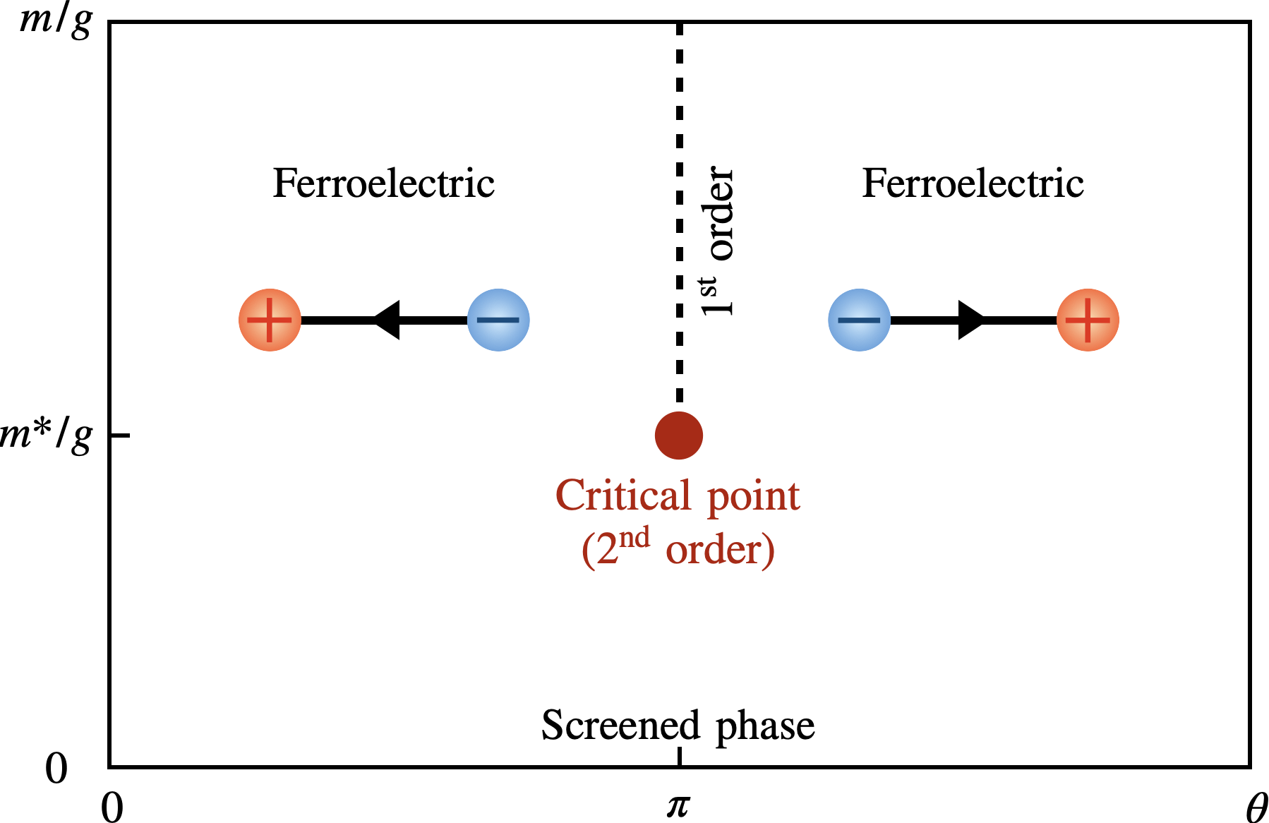
Figure 1: Phase diagram of the massive Schwinger model in the $(\theta,m/g)$ plane. At $\theta=\pi$ and large masses $m>m^{\ast}$, the ferroelectric phases with opposite orientations of electric field are separated by the line of the first order phase transition. This line terminates at $m^{\ast}\approx 0.33g$ at the critical point, where the phase transition is second order. For small masses $m\ll m^{\ast}$, the electric field is screened by the production of light fermion-antifermion pairs.

II Topological fluctuations near the critical point

Let us now discuss topological fluctuations in massive Schwinger model. For that purpose, it will be convenient to use the Hamiltonian formalism with the temporal gauge, $A_{0}=0$. From the action (2) the canonical momentum conjugate to $A_{1}$ can be read off as $\Pi=\dot{A}_{1}$. The corresponding Hamiltonian is then given by

$$H =\int\mathrm{d}x\left[\frac{1}{2}\Pi^{2}-\bar{\psi}(\mathrm{i}\gamma^{1}D_{1}-m\mathrm{e}^{\mathrm{i}\gamma_{5}\theta})\psi\right],$$ (3)

with commutation relations $[A_{1}(x),\Pi(y)]=\mathrm{i}\delta(x-y)$, and $\{\psi(x),\bar{\psi}(y)\}=\gamma_{0}\delta(x-y)$. In the bosonized description of the theory, the Hamiltonian is given by (see Appendix A for details)

$$\begin{split}H=\int\mathrm{d}x&\Big{[}\frac{1}{2}\dot{\varphi}^{2}+\frac{1}{2}(\partial_{1}{\varphi})^{2}+\frac{\mu^{2}}{2}\left(\varphi+\frac{\theta}{2\sqrt{\pi}}\right)^{2}\\ &-cm\mu\cos(2\sqrt{\pi}\varphi)\Big{]}.\end{split}$$ (4)

The potential of the model is thus given by

$$U(\varphi)=\frac{\mu^{2}}{2}\left(\varphi+\frac{\theta}{2\sqrt{\pi}}\right)^{2}-cm\mu\cos{(2\sqrt{\pi}\varphi)},$$ (5)

where $\mu=g/\sqrt{\pi}$ is the mass of the scalar boson, and the dimensionless coefficient $c$ is given by $c=\mathrm{e}^{\gamma}/2\pi$ with the Euler constant $\gamma=0.5774$. The electric field is related to the boson field as

$$E=-\mu\left(\varphi+\frac{\theta}{2\sqrt{\pi}}\right),$$ (6)

where the first term is the quantum, dynamical contribution and the second one is the classical background induced by the $\theta$ angle, $E_{\mathrm{cl}}=-g\theta/2\pi$.

The physics is periodic as a function of $\theta$ in the absence of boundaries – as $\theta$ increases, the electric field becomes capable of producing a fermion-antifermion pair (or kink-antikink pair, in bosonic description) that screens it. At $\theta=\pi$ the potential takes the form

$$U(\varphi)=\frac{\mu^{2}}{2}\left(\varphi+\frac{\sqrt{\pi}}{2}\right)^{2}-cm\mu\cos{(2\sqrt{\pi}\varphi)}.$$ (7)

When $m\gg\mu$, the potential has two well separated minima at $\varphi\approx 0,-\sqrt{\pi}$, associated with spontaneous symmetry breaking. As follows from (6), the minima $\varphi=0,-\sqrt{\pi}$ correspond to the electric fields $E=-g/2$ and $E=g/2$, respectively.

When $m\ll\mu$, there is a single minimum at $\varphi=-\sqrt{\pi}/2$, which according to (6) corresponds to the phase with no electric field. This is because at small $m$, the electric field is easily screened by the production of fermion-antifermion pairs - so we are dealing with the screened phase. At some critical value $m\approx m^{\ast}$, the effective potential becomes flat – this corresponds to the critical point with a second order phase transition. For $m>m^{\ast}$, the minima are separated by a potential barrier, and the transition between them (corresponding to the change in the direction of the electric dipole moment of the system) is first order – for example, having a domain with an opposite orientation of the electric dipole moment would cost an additional energy due to the “surface tension”. Due to this extra energy, the fluctuations of the electric dipole moment at $m\gg m^{\ast}$ are suppressed. At the critical point, where $m\approx m^{\ast}$, the potential barrier between the two minima disappears, and the “surface tension” of the domains with opposite orientations of the electric dipole moments vanishes. Because of this, the fluctuations of the electric dipole moment near the critical point are strongly enhanced. Here one can draw a useful analogy to the physics of ferroelectrics, where the electric susceptibility exhibits critical behavior near the Curie point [65].

When the ratio $m/g$ becomes very small, the electric field is easily screened by the production of fermion-antifermion pairs (or kink-antikink pairs in the bosonized description), and the fluctuations of electric dipole moment again become small. Basing on this qualitative picture (that we will confirm below with a more formal treatment), we expect to see a maximum in the electric susceptibility near the critical point. We will show that this is indeed the case.

In order to characterize the topological fluctuation we compute the static topological susceptibility. It is the zero frequency and wavelength limit of the real-time two-point correlation function of the topological charge:

$$\chi_{\text{CS}}$$

$$=\lim_{\omega\to 0}\lim_{k\to 0}\int\mathrm{d}^{2}x\,\mathrm{e}^{\mathrm{i}\omega t-\mathrm{i}kx}\big{[}\langle Q(x)Q(0)\rangle-\langle Q(x)\rangle\langle Q(0)\rangle\big{]}$$

$$=2\text{Re}\int\mathrm{d}^{2}x\Theta(t)\big{[}\langle Q(x)Q(0)\rangle-\langle Q(x)\rangle\langle Q(0)\rangle\big{]},$$ (8)

where $\Theta(t)$ is the Heaviside’s step function. $Q(x)=\partial_{\mu}K^{\mu}$ is the density of the Chern-Pontryagin number given by the divergence of the Chern-Simons current $K^{\mu}$. In $(1+1)$ dimensions, $K^{\mu}=(g/2\pi)\epsilon^{\mu\nu}A_{\nu}$, and $Q=(g/4\pi)\epsilon^{\mu\nu}F_{\mu\nu}$, where $F_{\mu\nu}$ is the electromagnetic field strength tensor. The corresponding change of Chern-Simons number is $\Delta N_{\mathrm{CS}}=\int\mathrm{d}^{2}xK^{0}=(g/2\pi)\int\mathrm{d}^{2}xA_{1}$; the Chern-Pontryagin number density is given by the electric field: $Q(x)=(g/2\pi)E(x)$. We call $\chi_{\text{CS}}$ (II) the real-time topological susceptibility because it is computed from the real-time two-point function unlike the conventional topological susceptibility which is computed in the Euclidean space-time.

III Lattice Schwinger model

III.1 Lattice Hamiltonian

For the purpose of numerical simulation, we place the theory (3) on a spatial lattice. We introduce the staggered fermion $\chi_{n}$ and $\chi^{\dagger}_{n}$ [66, 67], and lattice gauge field operators $L_{n}$ and $U_{n}$ with an integer $n$ labeling a lattice site; the lattice spacing is $a$. A two-component Dirac fermion $\psi=(\psi^{1},\psi^{2})^{T}$ is converted to a staggered fermion $\psi^{1}(\psi^{2})\to\chi_{n}/\sqrt{a}$ for odd (even) $n$. The gauge fields are replaced by $\mathrm{e}^{-\mathrm{i}agA_{1}}\to U_{n}$ and $\Pi\to-gL_{n}$, that are placed on a link between $n$th and $(n+1)$st sites. The resulting lattice Hamiltonian is,

$$H =\frac{ag^{2}}{2}\sum_{n=1}^{N-1}L_{n}^{2}-\frac{\mathrm{i}}{2a}\sum_{n=1}^{N-1}\big{[}\chi^{\dagger}_{n+1}U_{n}\chi_{n}-\chi^{\dagger}_{n}U_{n}^{\dagger}\chi_{n+1}\big{]}$$

$$+m\cos\theta\sum_{n=1}^{N}(-1)^{n}\chi^{\dagger}_{n}\chi_{n}$$

$$+\mathrm{i}\frac{m\sin\theta}{2}\sum_{n=1}^{N-1}(-1)^{n}\big{[}\chi^{\dagger}_{n+1}U_{n}\chi_{n}-\chi^{\dagger}_{n}U_{n}^{\dagger}\chi_{n+1}\big{]},$$ (9)

with the Gauss law constraint:

$$L_{n+1}-L_{n}=\chi_{n}^{\dagger}\chi_{n}-\frac{1-(-1)^{n}}{2}.$$ (10)

The right-hand side corresponds to the fermion density in terms of the Dirac fermions $\psi$. The second term reflects the fact that each component of Dirac fermion $\psi_{1}$ ($\psi_{2}$) is translated to a staggered fermion on odd (even) $n$. We solve the constraint to eliminate the electric field operators,

$$L_{n}=\sum_{i=1}^{n}\left(\chi_{i}^{\dagger}\chi_{i}-\frac{1-(-1)^{i}}{2}\right),$$ (11)

where we have fixed the boundary electric field, $L_{0}=0$. By enforcing the relation (11), the states are automatically restricted to the physical ones. We furthermore eliminate the link fields $U_{n}$ by the gauge transformation,

$$\chi_{n}\to g_{n}\chi_{n},\quad\chi^{\dagger}_{n}\to\chi^{\dagger}_{n}g_{n}^{\dagger},\quad U_{n}\to g_{n+1}U_{n}g_{n}^{\dagger},$$ (12)

with

$$g_{1}=1,\quad g_{n}=\prod_{i=1}^{n-1}U^{\dagger}_{i}.$$ (13)

In the present work, we limit $\theta$ to be $0$ or $\pi$ to study the critical behavior at $\theta=\pi$. Upon absorbing $\cos\theta=\pm 1$ in the second line of (III.1) to the fermion mass $m$, we arrive at the Hamiltonian,

$$\begin{split}H&=\frac{ag^{2}}{2}\sum_{n=1}^{N-1}\left[\sum_{i=1}^{n}\left(\chi_{i}^{\dagger}\chi_{i}-\frac{1-(-1)^{i}}{2}\right)\right]^{2}\\ &-\frac{\mathrm{i}}{2a}\sum_{n=1}^{N-1}\big{[}\chi^{\dagger}_{n+1}\chi_{n}-\chi^{\dagger}_{n}\chi_{n+1}\big{]}\\ &+m\sum_{n=1}^{N}(-1)^{n}\chi^{\dagger}_{n}\chi_{n}.\end{split}$$ (14)

It is noted again that the massive theory with a positive mass $m>0$ at $\theta=\pi$ is equivalent to the theory at $\theta=0$ but with a negative mass $-m$. The Hamiltonian (14) accords with the latter viewpoint and will be used in what follows. Note that the method used here is not restricted to $\theta=0$ and $\pi$ but can be generalized to other values of $\theta$ without any difficulty.

III.2 Real-time topological susceptibility

We compute the real-time topological susceptibility,

$$\chi_{\text{CS}}=2\left(\frac{g}{2\pi}\right)^{2}\text{Re}\int\mathrm{d}^{2}x\Theta(t)\big{[}\langle E(x)E(0)\rangle-\langle E(x)\rangle\langle E(0)\rangle\big{]},$$ (15)

where $\Theta(t)$ is the Heaviside step function. Recall that the Chern-Pontyagin number density is proportional to the electric field in 1+1 dimensions (II). For the purpose of calculating the topological susceptibility we take the zero-wavelength limit followed by the zero-frequency limit,

$$\begin{split}&\chi_{\text{CS}}=2\left(\frac{g}{2\pi}\right)^{2}V\text{Re}\int\mathrm{d}t\Theta(t)(\langle\bar{E}(t)\bar{E}(0)\rangle-\langle\bar{E}(0)\rangle^{2}),\end{split}$$ (16)

where $V$ is spatial volume (length) and $\bar{E}(t):=\int\mathrm{d}xE(t,x)/V$ is spatial average of electric field operator. We have used the translational invariance both in temporal and spatial directions, which approximately holds in a finite-size system.

On a lattice, it is given by

$$\chi_{\text{CS}}=2(N-1)\left(\frac{g}{2\pi}\right)^{2}ag^{2}$$

$$\times\mathrm{Re}\int_{0}^{T}\mathrm{d}t\Theta(t)(\langle\bar{L}(t)\bar{L}(0)\rangle-\langle\bar{L}(0)\rangle^{2}).$$ (17)

with $\bar{L}:=\frac{1}{N-1}\sum_{n=1}^{N-1}L_{n}$. Note that the temporal integral is also truncated by $T$ (not to be confused with temperature). We numerically compute the dimensionless topological susceptibility,

$$\frac{\chi_{\text{CS}}}{g^{2}}=\frac{N-1}{\pi^{2}}\mathrm{Re}\int_{0}^{\hat{T}}\mathrm{d}\hat{t}(t)(\langle\bar{L}(t)\bar{L}(0)\rangle-\langle\bar{L}(0)\rangle^{2}).$$ (18)

with the dimensionless variables $\hat{t}:=(ag^{2}/2)t$ and $\hat{T}:=(ag^{2}/2)T$.

IV Results and discussion

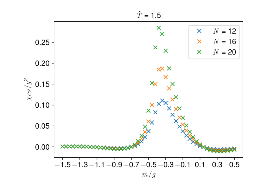
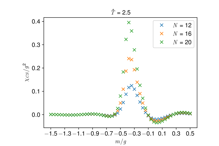
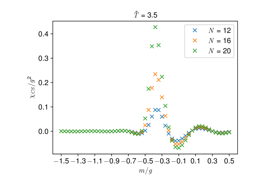
Figure 2: Dimensionless real-time topological susceptibility $\chi_{\text{CS}}/g^{2}$ as function of $m/g$ at different values of lattice size $N$ and range of temporal integral $\hat{T}=(ag^{2}/2)T$. The topological susceptibility is computed using the Hamiltonian (14), where $\theta$ is limited to $0$ or $\pi$.

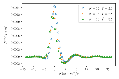
Figure 3: Rescaled dimensionless real-time topological susceptibility $N^{-7/4}\chi/g^{2}$ as functions of $N(m-m^{\ast})/g$ at different values of lattice size $N$. The temporal range $\hat{T}=(ag^{2}/2)T$ is taken to be proportional to $N$. The topological susceptibility is computed using the Hamiltonian (14), where $\theta$ is limited to $0$ or $\pi$.

We have numerically computed the susceptibility (18) using a Python package QuSpin [68, 69]. For the purpose of numerical analysis we convert the lattice Hamiltonian of the Schwinger model to the spin Hamiltonian via the Jordan-Wigner transformation (Appendix B). The same Hamiltonian can be directly used to implement the digital quantum simulation of the Schwinger model.

The real-time topological susceptibilities are shown in Fig. 2 as functions of $m/g$ for different values of time $\hat{T}$ and lattice size $N$. The data exhibits a sharp peak around the critical masses $m^{\ast}/g\approx-0.33$. In order to confirm the critical behavior we plot in Fig. 3 the rescaled susceptibility

$$\quad N^{-7/4}\chi_{\text{CS}}/g^{2},$$ (19)

as a function of $N(m-m^{\ast})/g$, based on the finite-size scaling analysis detailed in Appendix C. We set $m^{\ast}/g=-0.33$ in accord with previous studies [60, 61, 62]. Here, the temporal integral range $\hat{T}$ is taken to be proportional to the spatial lattice size $N$.

The dependence of the susceptibility on the lattice size can be understood using the finite-size scaling, with the critical exponents of the transverse Ising model. The $Z_{2}$ symmetry of lattice Schwinger model at $\theta=\pi$ and broken parity put it in the same universality class as the $1+1$ dimensional transverse-field Ising model, which in turn is equivalent to 2D Euclidean classical Ising model. The corresponding finite-size scaling analysis is explained in the Appendix C.

The sharp peak in the real-time topological susceptibility near the critical point of the phase diagram may have important implications for the search for the critical point of the QCD phase diagram. It has been argued [70, 63] that the behavior near the critical point in the QCD phase diagram belongs to the universality class of 3D Ising model. The model that we have studied in the paper belongs to the universality class of 2D classical Ising model that is characterized by different critical exponents, but shares many common features with the 3D Ising model.

In particular, we expect that the sharp peak in real-time susceptibility that we have observed near the critical point will also be present in the 3D Ising model, and thus near the critical point in QCD phase diagram. This would imply strong fluctuations of topological charge near the critical point, that can be detected through the charged hadron asymmetries  [57, 71, 72] that are currently under intense studies at RHIC.

The critical behavior in the model that we have studied belongs to the universality class of model A, in the Hohenberg-Halperin classification [73]. Therefore, we expect that our findings apply to a broad class of physical systems, including those described by the kinetic Ising models [74]. These models are widely used to describe the relaxational processes in near-equilibrium states, and our study of the real-time critical fluctuations contributes to the field in two different ways.

First, we show how to use the Hamiltonian formalism of quantum field theory in this problem. This formalism is suitable for digital quantum simulations, and opens the pathway towards the study of these non-equilibrium phenomena on future quantum computers. It would be particularly beneficial for the future studies of higher dimensional or more complicated theories such as QCD, where real-time simulations on classical computers are very challenging.

Second, we demonstrate that close to the critical point the topological susceptibility exhibits a sharp peak. In our case, the topological susceptibility describes the fluctuations of Chern-Simons number, and in other models in the same universality class, such as anisotropic magnets, it would describe the magnetic susceptibility.

The similarity to ferroelectrics may allow one to simulate the real-time ferroelectric response near the critical point [65]. Given the importance of ferroelectrics for information storage and processing [75], this may have interesting practical applications.

Appendix A Massive Schwinger model at finite $\theta$

We review the massive Schwinger model at finite $\theta$ (see e.g. [76] for a comprehensive review). Let us start with 1+1D Maxwell theory at finite $\theta$:

$$S=\int\mathrm{d}^{2}x\left(\frac{1}{2}E^{2}+\frac{g\theta}{2\pi}E\right),$$ (20)

where $E=F_{01}=\partial_{0}A_{1}=\dot{A}_{1}$ is an electric field and the temporal gauge $A_{0}=0$ is taken. The momentum $\Pi$ conjugate to $A_{1}$ is,

$$\Pi=\dot{A}_{1}+\frac{g\theta}{2\pi},$$ (21)

obeying $[\Pi(x),A_{1}(y)]=\mathrm{i}\delta(x-y)$. Hence, the Hamiltonian density takes the form,

$$\mathcal{H}=\Pi\dot{A}-\left(\frac{1}{2}E^{2}+\frac{g\theta}{2\pi}E\right)=\frac{1}{2}\left(\Pi-\frac{g\theta}{2\pi}\right)^{2}.$$ (22)

The Gauss operator must vanish,

$$\partial_{1}\Pi=0,$$ (23)

on physical states. Therefore, $\Pi$ is fixed once its value is specified, $\Pi|_{\text{boundary}}=\epsilon_{0}$, at one of the two boundaries. The boundary value $\epsilon_{0}$ is interpreted as a background electric field. Hereafter, we take $\epsilon_{0}=0$ with the background electric field being absorbed into $\theta$.

We now add a dynamical Dirac fermion $\psi$ to have,

$$S=\int\mathrm{d}^{2}x\left(\frac{1}{2}E^{2}+\frac{g\theta}{2\pi}E\right)+\bar{\psi}(\mathrm{i}\not{D}-m)\psi.$$ (24)

Then, the Gauss law fixes the electric field in the bulk as

$$\Pi=g\int_{\mathrm{boundary}}^{x}\mathrm{d}y\ \psi^{\dagger}\psi(y),$$ (25)

where $\epsilon_{0}=0$ is taken. We call $\Pi$ the dynamical electric field because it is induced by fermionic excitations as opposed to $E=\dot{A_{1}}=\Pi-g\theta/(2\pi)$, where the second term represents the background electric field.

In line with the main text, we will briefly describe the bosonized form of the theory. The bosonization dictionary is as follows:

$$\begin{split}\mathrm{i}\bar{\psi}\gamma^{\mu}\partial_{\mu}\psi\quad&\leftrightarrow\quad\frac{(\partial_{\mu}\varphi)^{2}}{2},\\ \bar{\psi}\gamma^{\mu}\psi\quad&\leftrightarrow\quad-\frac{\epsilon^{\mu\nu}\partial_{\nu}\varphi}{\sqrt{\pi}},\\ \bar{\psi}\gamma^{\mu}\gamma_{5}\psi\quad&\leftrightarrow\quad-\frac{\partial_{\mu}\varphi}{\sqrt{\pi}},\\ \bar{\psi}\psi\quad&\leftrightarrow\quad-\frac{cg}{\sqrt{\pi}}\cos(2\sqrt{\pi}\varphi),\end{split}$$ (26)

with a dimensionless constant $c=\mathrm{e}^{\gamma}/(2\pi)$ and the Euler constant $\gamma$. Therefore, the action (24) is converted to

$$\begin{split}S&=\int\mathrm{d}^{2}x\Big{[}\frac{1}{2}E^{2}+\frac{g\theta}{2\pi}E\\ &+\frac{(\partial_{\mu}\varphi)^{2}}{2}+gA_{\mu}\frac{\epsilon^{\mu\nu}\partial_{\nu}\varphi}{\sqrt{\pi}}+\frac{cmg}{\sqrt{\pi}}\cos(2\sqrt{\pi}\varphi)\Big{]}\\ &=\int\mathrm{d}^{2}x\Big{[}\frac{1}{2}E^{2}+\frac{g}{2\pi}(2\sqrt{\pi}\varphi+\theta)E\\ &+\frac{(\partial_{\mu}\varphi)^{2}}{2}+\frac{cmg}{\sqrt{\pi}}\cos(2\sqrt{\pi}\varphi)\Big{]}.\end{split}$$ (27)

The equation of motion for $\varphi$ yields,

$$\partial^{2}\varphi=\frac{g}{\sqrt{\pi}}E-2cmg\sin(2\sqrt{\pi}\varphi),$$ (28)

which, at $m=0$, turns out to be the anomaly equation for the axial current $j^{\mu}_{5}=\bar{\psi}\gamma^{\mu}\gamma_{5}\psi$. The equation of motion for $A_{1}$ yields,

$$\partial_{1}\left(E+g\frac{2\sqrt{\pi}\varphi+\theta}{2\pi}\right)=0.$$ (29)

By requiring the quantity inside the parenthesis to vanish at spatial infinity, we find

$$E=-g\frac{2\sqrt{\pi}\varphi+\theta}{2\pi}.$$ (30)

Using the equation of motion, or equivalently integrating out the gauge field, we get the pure bosonic action,

$$\begin{split}S=\int\mathrm{d}^{2}x\Big{[}&\frac{(\partial_{\mu}\varphi)^{2}}{2}-\frac{g^{2}}{8\pi^{2}}(2\sqrt{\pi}\varphi+\theta)^{2}\\ &+\frac{cmg}{\sqrt{\pi}}\cos(2\sqrt{\pi}\varphi)\Big{]}.\end{split}$$ (31)

For $4\pi m>g/(\sqrt{\pi}c)$, at $\theta=\pi$ there exist the degenerate ground states for $\varphi$ satisfying,

$$\frac{cmg}{\sqrt{\pi}}\sin(2\sqrt{\pi}\varphi)=\frac{g^{2}}{4\pi^{2}}(2\sqrt{\pi}\varphi+\pi).$$ (32)

Given the two solutions $\varphi=(-\pi\pm\mathcal{E})/(2\sqrt{\pi})$ with some value $\mathcal{E}$, we find the associated total electric fields

$$E=\pm g\frac{\mathcal{E}}{2\pi},$$ (33)

respectively. For $m\gg g$, $\mathcal{E}$ approaches $\pi$ and thus the total electric field $E$ approximately takes the values $\pm g/2$.

Appendix B Spin Hamiltonian of the Schwinger model

We show the spin Hamiltonin used for the numerical simulation presented in the main text and for the purpose of implementing digital quantum simulation. We employ the Jordan-Wigner transformation [77]

$$\begin{split}\chi_{n}&=\frac{X_{n}-\mathrm{i}Y_{n}}{2}\prod_{i=1}^{n-1}(-\mathrm{i}Z_{i}),\\ \chi^{\dagger}_{n}&=\frac{X_{n}+\mathrm{i}Y_{n}}{2}\prod_{i=1}^{n-1}(\mathrm{i}Z_{i}),\end{split}$$ (34)

to convert the Hamiltonian of the massive Schwinger model to the following spin Hamiltonian [78],

$$\begin{split}H=&\frac{1}{4a}\sum_{n=1}^{N-1}(X_{n}X_{n+1}+Y_{n}Y_{n+1})+\frac{m}{2}\sum_{n=1}^{N}(-1)^{n}Z_{n}\\ &+\frac{ag^{2}}{2}\sum_{n=1}^{N}\left(\sum_{i=1}^{n}\frac{Z_{i}+(-1)^{i}}{2}\right)^{2}.\end{split}$$ (35)

The last term is the gauge kinetic term with the electric field given by

$$L_{n}=\sum_{i=1}^{n}\frac{Z_{i}+(-1)^{i}}{2},$$ (36)

which is uniquely fixed by the Gauss law

$$L_{n+1}-L_{n}=\frac{Z_{n+1}+(-1)^{n+1}}{2}$$ (37)

upon fixing the boundary electric field to $0$.

Appendix C Finite-volume analysis

We are interested in computing the static susceptibility in the Schwinger model,

$$\chi(m):=\lim_{\omega\to 0}\lim_{k\to 0}\chi(k,\omega,m),$$ (38)

where $\chi(k,\omega;m)$ is the retarded Green’s function of electric fields. In 1+1 dimensional systems, the electric field can be regarded as a topological charge density $E=F_{01}$.

In the thermodynamic limit the Green’s function is expected to diverge at the quantum critical point. It is, however, not divergent in finite volume with the system size $N$. Hence, we attempt to identify the critical points, specified by the fermion mass $m^{\ast}$, by fitting the regularized Green’s function $\tilde{\chi}(m;N)$.

Around the critical point $\Delta m:=m-m^{\ast}\sim 0$, the susceptibility behaves as [79],

$$\chi(m)\approx A|\Delta m|^{-\gamma}.$$ (39)

In a finite system of size $L=Na$, the susceptibility is

$$\tilde{\chi}(m;N)\approx N^{\gamma/\nu}Q(N/\xi),$$ (40)

with the scaling function $Q$ and the correlation length $\xi$ given by

$$\xi(m)\approx\xi_{0}|\Delta m|^{-\nu}.$$ (41)

The ansatz (40) is satisfied in the limit $N\to\infty$ by requiring

$$Q(x)\approx A(\xi_{0}x)^{-\gamma/\nu}\qquad x\to\infty.$$ (42)

Note the scaling relation can be read off from the relation between the susceptibility and correlation length (Sec.4 in [80]),

$$\chi\sim\xi^{2-\eta}.$$ (43)

Combined with (39) and (41) we find the scaling relation

$$\gamma=\nu(2-\eta).$$ (44)

The criticality of lattice Schwinger model belongs to the same universality class as 1+1D transverse Ising model, which in turn equivalent to 2D classical Ising model. Hence the critical exponents are,

$$\gamma=\frac{7}{4},\qquad\eta=\frac{1}{4},\qquad\nu=1.$$ (45)

Finally, the relation (40) in a finite system becomes $N$-independent if we use the following rescaled quantities:

$$N^{1/\nu}\Delta m=N\Delta m,\quad N^{-\gamma/\nu}\tilde{\chi}=N^{-7/4}\tilde{\chi}.$$ (46)

Indeed, the data points with different lattice size $N$ approximately collapse as shown in Fig. 3. The susceptibility $\tilde{\chi}$ corresponds to $\chi_{\text{CS}}$ in the main text.

References

- [1] J. S. Schwinger, “Gauge Invariance and Mass,” Phys. Rev. 125 (1962) 397–398. [,151(1962)].
- [2] L. Brown, “Gauge invariance and mass in a two-dimensional model,” Il Nuovo Cimento (1955-1965) 29 no. 3, (1963) 617–643.
- [3] C. M. Sommerfield, “On the definition of currents and the action principle in field theories of one spatial dimension,” Annals of Physics 26 no. 1, (1964) 1–43.
- [4] B. Zumino, “Charge conservation and the mass of the photon,” Phys. Lett. 10 no. CERN-TH-425, (1964) 224–226.
- [5] C. Hagen, “Current definition and mass renormalization in a model field theory,” Il Nuovo Cimento A (1965-1970) 51 no. 4, (1967) 1033–1052.
- [6] J. Lowenstein and J. Swieca, “Quantum electrodynamics in two dimensions,” Annals of Physics 68 no. 1, (1971) 172–195.
- [7] A. Casher, J. Kogut, and L. Susskind, “Vacuum polarization and the absence of free quarks,” Physical Review D 10 no. 2, (1974) 732.
- [8] S. Coleman, R. Jackiw, and L. Susskind, “Charge shielding and quark confinement in the massive schwinger model,” Annals of Physics 93 no. 1-2, (1975) 267–275.
- [9] A. Wallraff, D. I. Schuster, A. Blais, L. Frunzio, R. S. Huang, J. Majer, S. Kumar, S. M. Girvin, and R. J. Schoelkopf, “Strong coupling of a single photon to a superconducting qubit using circuit quantum electrodynamics,” Nature 431 no. 7005, (2004) 162–167.
- [10] J. Majer, J. M. Chow, J. M. Gambetta, J. Koch, B. R. Johnson, J. A. Schreier, L. Frunzio, D. I. Schuster, A. A. Houck, A. Wallraff, A. Blais, M. H. Devoret, S. M. Girvin, and R. J. Schoelkopf, “Coupling superconducting qubits via a cavity bus,” Nature 449 no. 7161, (2007) 443–447.
- [11] S. P. Jordan, K. S. M. Lee, and J. Preskill, “Quantum Algorithms for Quantum Field Theories,” Science 336 (2012) 1130–1133, arXiv:1111.3633 [quant-ph].
- [12] S. P. Jordan, K. S. M. Lee, and J. Preskill, “Quantum Computation of Scattering in Scalar Quantum Field Theories,” arXiv:1112.4833 [hep-th]. [Quant. Inf. Comput.14,1014(2014)].
- [13] E. Zohar, J. I. Cirac, and B. Reznik, “Simulating Compact Quantum Electrodynamics with ultracold atoms: Probing confinement and nonperturbative effects,” Phys. Rev. Lett. 109 (2012) 125302, arXiv:1204.6574 [quant-ph].
- [14] E. Zohar, J. I. Cirac, and B. Reznik, “Cold-Atom Quantum Simulator for SU(2) Yang-Mills Lattice Gauge Theory,” Phys. Rev. Lett. 110 no. 12, (2013) 125304, arXiv:1211.2241 [quant-ph].
- [15] D. Banerjee, M. Bögli, M. Dalmonte, E. Rico, P. Stebler, U. J. Wiese, and P. Zoller, “Atomic Quantum Simulation of U(N) and SU(N) Non-Abelian Lattice Gauge Theories,” Phys. Rev. Lett. 110 no. 12, (2013) 125303, arXiv:1211.2242 [cond-mat.quant-gas].
- [16] D. Banerjee, M. Dalmonte, M. Muller, E. Rico, P. Stebler, U. J. Wiese, and P. Zoller, “Atomic Quantum Simulation of Dynamical Gauge Fields coupled to Fermionic Matter: From String Breaking to Evolution after a Quench,” Phys. Rev. Lett. 109 (2012) 175302, arXiv:1205.6366 [cond-mat.quant-gas].
- [17] U.-J. Wiese, “Ultracold Quantum Gases and Lattice Systems: Quantum Simulation of Lattice Gauge Theories,” Annalen Phys. 525 (2013) 777–796, arXiv:1305.1602 [quant-ph].
- [18] U.-J. Wiese, “Towards Quantum Simulating QCD,” Nucl. Phys. A931 (2014) 246–256, arXiv:1409.7414 [hep-th].
- [19] S. P. Jordan, K. S. M. Lee, and J. Preskill, “Quantum Algorithms for Fermionic Quantum Field Theories,” arXiv:1404.7115 [hep-th].
- [20] L. García-Álvarez, J. Casanova, A. Mezzacapo, I. L. Egusquiza, L. Lamata, G. Romero, and E. Solano, “Fermion-Fermion Scattering in Quantum Field Theory with Superconducting Circuits,” Phys. Rev. Lett. 114 no. 7, (2015) 070502, arXiv:1404.2868 [quant-ph].
- [21] D. Marcos, P. Widmer, E. Rico, M. Hafezi, P. Rabl, U. J. Wiese, and P. Zoller, “Two-dimensional Lattice Gauge Theories with Superconducting Quantum Circuits,” Annals Phys. 351 (2014) 634–654, arXiv:1407.6066 [quant-ph].
- [22] A. Bazavov, Y. Meurice, S.-W. Tsai, J. Unmuth-Yockey, and J. Zhang, “Gauge-invariant implementation of the Abelian Higgs model on optical lattices,” Phys. Rev. D92 no. 7, (2015) 076003, arXiv:1503.08354 [hep-lat].
- [23] E. Zohar, J. I. Cirac, and B. Reznik, “Quantum Simulations of Lattice Gauge Theories using Ultracold Atoms in Optical Lattices,” Rept. Prog. Phys. 79 no. 1, (2016) 014401, arXiv:1503.02312 [quant-ph].
- [24] A. Mezzacapo, E. Rico, C. Sabín, I. L. Egusquiza, L. Lamata, and E. Solano, “Non-Abelian Lattice Gauge Theories in Superconducting Circuits,” Phys. Rev. Lett. 115 no. 24, (2015) 240502, arXiv:1505.04720 [quant-ph].
- [25] M. Dalmonte and S. Montangero, “Lattice gauge theory simulations in the quantum information era,” Contemp. Phys. 57 no. 3, (2016) 388–412, arXiv:1602.03776 [cond-mat.quant-gas].
- [26] E. Zohar, A. Farace, B. Reznik, and J. I. Cirac, “Digital lattice gauge theories,” Phys. Rev. A95 no. 2, (2017) 023604, arXiv:1607.08121 [quant-ph].
- [27] E. A. Martinez et al., “Real-time dynamics of lattice gauge theories with a few-qubit quantum computer,” Nature 534 (2016) 516–519, arXiv:1605.04570 [quant-ph].
- [28] A. Bermudez, G. Aarts, and M. Müller, “Quantum sensors for the generating functional of interacting quantum field theories,” Phys. Rev. X7 no. 4, (2017) 041012, arXiv:1704.02877 [quant-ph].
- [29] J. M. Gambetta, J. M. Chow, and M. Steffen, “Building logical qubits in a superconducting quantum computing system,” npj Quantum Information 3 no. 1, (2017) 2.
- [30] L. Krinner, M. Stewart, A. Pazmiño, J. Kwon, and D. Schneble, “Spontaneous emission of matter waves from a tunable open quantum system,” Nature 559 no. 7715, (2018) 589–592.
- [31] A. Macridin, P. Spentzouris, J. Amundson, and R. Harnik, “Electron-Phonon Systems on a Universal Quantum Computer,” Phys. Rev. Lett. 121 no. 11, (2018) 110504, arXiv:1802.07347 [quant-ph].
- [32] T. V. Zache, F. Hebenstreit, F. Jendrzejewski, M. K. Oberthaler, J. Berges, and P. Hauke, “Quantum simulation of lattice gauge theories using Wilson fermions,” Sci. Technol. 3 (2018) 034010, arXiv:1802.06704 [cond-mat.quant-gas].
- [33] J. Zhang, J. Unmuth-Yockey, J. Zeiher, A. Bazavov, S. W. Tsai, and Y. Meurice, “Quantum simulation of the universal features of the Polyakov loop,” Phys. Rev. Lett. 121 no. 22, (2018) 223201, arXiv:1803.11166 [hep-lat].
- [34] N. Klco, E. F. Dumitrescu, A. J. McCaskey, T. D. Morris, R. C. Pooser, M. Sanz, E. Solano, P. Lougovski, and M. J. Savage, “Quantum-classical computation of Schwinger model dynamics using quantum computers,” Phys. Rev. A98 no. 3, (2018) 032331, arXiv:1803.03326 [quant-ph].
- [35] N. Klco and M. J. Savage, “Digitization of scalar fields for quantum computing,” Phys. Rev. A99 no. 5, (2019) 052335, arXiv:1808.10378 [quant-ph].
- [36] H.-H. Lu et al., “Simulations of Subatomic Many-Body Physics on a Quantum Frequency Processor,” Phys. Rev. A100 no. 1, (2019) 012320, arXiv:1810.03959 [quant-ph].
- [37] N. Klco and M. J. Savage, “Minimally-Entangled State Preparation of Localized Wavefunctions on Quantum Computers,” arXiv:1904.10440 [quant-ph].
- [38] H. Lamm and S. Lawrence, “Simulation of Nonequilibrium Dynamics on a Quantum Computer,” Phys. Rev. Lett. 121 no. 17, (2018) 170501, arXiv:1806.06649 [quant-ph].
- [39] E. Gustafson, Y. Meurice, and J. Unmuth-Yockey, “Quantum simulation of scattering in the quantum Ising model,” Phys. Rev. D99 no. 9, (2019) 094503, arXiv:1901.05944 [hep-lat].
- [40] N. Klco, J. R. Stryker, and M. J. Savage, “SU(2) non-Abelian gauge field theory in one dimension on digital quantum computers,” arXiv:1908.06935 [quant-ph].
- [41] NuQS Collaboration, A. Alexandru, P. F. Bedaque, H. Lamm, and S. Lawrence, “ Models on Quantum Computers,” Phys. Rev. Lett. 123 no. 9, (2019) 090501, arXiv:1903.06577 [hep-lat].
- [42] NuQS Collaboration, A. Alexandru, P. F. Bedaque, S. Harmalkar, H. Lamm, S. Lawrence, and N. C. Warrington, “Gluon Field Digitization for Quantum Computers,” Phys. Rev. D100 no. 11, (2019) 114501, arXiv:1906.11213 [hep-lat].
- [43] N. Mueller, A. Tarasov, and R. Venugopalan, “Deeply inelastic scattering structure functions on a hybrid quantum computer,” arXiv:1908.07051 [hep-th].
- [44] NuQS Collaboration, H. Lamm, S. Lawrence, and Y. Yamauchi, “Parton Physics on a Quantum Computer,” arXiv:1908.10439 [hep-lat].
- [45] G. Magnifico, M. Dalmonte, P. Facchi, S. Pascazio, F. V. Pepe, and E. Ercolessi, “Real Time Dynamics and Confinement in the Schwinger-Weyl lattice model for 1+1 QED,” arXiv:1909.04821 [quant-ph].
- [46] B. Chakraborty, M. Honda, T. Izubuchi, Y. Kikuchi, and A. Tomiya, “Digital Quantum Simulation of the Schwinger Model with Topological Term via Adiabatic State Preparation,” arXiv:2001.00485 [hep-lat].
- [47] D. E. Kharzeev and Y. Kikuchi, “Real-time chiral dynamics from a digital quantum simulation,” Phys. Rev. Res. 2 no. 2, (2020) 023342, arXiv:2001.00698 [hep-ph].
- [48] A. F. Shaw, P. Lougovski, J. R. Stryker, and N. Wiebe, “Quantum Algorithms for Simulating the Lattice Schwinger Model,” arXiv:2002.11146 [quant-ph].
- [49] B. Şahinoğlu and R. D. Somma, “Hamiltonian simulation in the low energy subspace,” arXiv:2006.02660 [quant-ph].
- [50] D. Paulson et al., “Towards simulating 2D effects in lattice gauge theories on a quantum computer,” arXiv:2008.09252 [quant-ph].
- [51] S. V. Mathis, G. Mazzola, and I. Tavernelli, “Toward scalable simulations of Lattice Gauge Theories on quantum computers,” Phys. Rev. D 102 no. 9, (2020) 094501, arXiv:2005.10271 [quant-ph].
- [52] NuQS Collaboration, Y. Ji, H. Lamm, and S. Zhu, “Gluon Field Digitization via Group Space Decimation for Quantum Computers,” arXiv:2005.14221 [hep-lat].
- [53] I. Raychowdhury and J. R. Stryker, “Loop, string, and hadron dynamics in SU(2) Hamiltonian lattice gauge theories,” Phys. Rev. D 101 no. 11, (2020) 114502, arXiv:1912.06133 [hep-lat].
- [54] Z. Davoudi, I. Raychowdhury, and A. Shaw, “Search for Efficient Formulations for Hamiltonian Simulation of non-Abelian Lattice Gauge Theories,” arXiv:2009.11802 [hep-lat].
- [55] R. Dasgupta and I. Raychowdhury, “Cold Atom Quantum Simulator for String and Hadron Dynamics in Non-Abelian Lattice Gauge Theory,” arXiv:2009.13969 [hep-lat].
- [56] G. Magnifico, D. Vodola, E. Ercolessi, S. P. Kumar, M. Müller, and A. Bermudez, “Symmetry-protected topological phases in lattice gauge theories: Topological QED2,” Phys. Rev. D 99 no. 1, (Jan., 2019) 014503, arXiv:1804.10568 [cond-mat.quant-gas].
- [57] D. Kharzeev, “Parity violation in hot QCD: Why it can happen, and how to look for it,” Phys. Lett. B633 (2006) 260–264, arXiv:hep-ph/0406125 [hep-ph].
- [58] K. Fukushima, D. E. Kharzeev, and H. J. Warringa, “Chiral magnetic effect,” Physical Review D 78 no. 7, (2008) 074033.
- [59] S. Coleman, “More about the massive schwinger model,” Annals of Physics 101 no. 1, (1976) 239–267.
- [60] A. Schiller and J. Ranft, “The massive schwinger model on the lattice studied via a local hamiltonian monte carlo method,” Nuclear Physics B 225 no. 2, (1983) 204–220.
- [61] C. Hamer, J. Kogut, D. Crewther, and M. Mazzolini, “The massive schwinger model on a lattice: Background field, chiral symmetry and the string tension,” Nuclear Physics B 208 no. 3, (1982) 413–438.
- [62] T. Byrnes, P. Sriganesh, R. Bursill, and C. Hamer, “Density matrix renormalization group approach to the massive schwinger model,” Physical Review D 66 no. 1, (2002) 013002.
- [63] K. Rajagopal and F. Wilczek, “The condensed matter physics of qcd,” in At The Frontier of Particle Physics: Handbook of QCD (In 3 Volumes), pp. 2061–2151. World Scientific, 2001.
- [64] M. A. Stephanov, “QCD phase diagram and the critical point,” Prog. Theor. Phys., Suppl. 153 no. hep-ph/0402115, (2004) 139–156.
- [65] S. Rowley, L. Spalek, R. Smith, M. Dean, M. Itoh, J. Scott, G. Lonzarich, and S. Saxena, “Ferroelectric quantum criticality,” Nature Physics 10 no. 5, (2014) 367–372.
- [66] J. B. Kogut and L. Susskind, “Hamiltonian Formulation of Wilson’s Lattice Gauge Theories,” Phys. Rev. D11 (1975) 395–408.
- [67] L. Susskind, “Lattice Fermions,” Phys. Rev. D16 (1977) 3031–3039.
- [68] P. Weinberg and M. Bukov, “QuSpin: a Python Package for Dynamics and Exact Diagonalisation of Quantum Many Body Systems part I: spin chains,” SciPost Phys. 2 (2017) 003.
- [69] P. Weinberg and M. Bukov, “QuSpin: a Python package for dynamics and exact diagonalisation of quantum many body systems. Part II: bosons, fermions and higher spins,” SciPost Phys. 7 no. arXiv: 1804.06782, (2019) 020.
- [70] M. Halasz, A. Jackson, R. Shrock, M. A. Stephanov, and J. Verbaarschot, “Phase diagram of qcd,” Physical Review D 58 no. 9, (1998) 096007.
- [71] D. E. Kharzeev, L. D. McLerran, and H. J. Warringa, “The effects of topological charge change in heavy ion collisions:“event by event p and cp violation”,” Nuclear Physics A 803 no. 3-4, (2008) 227–253.
- [72] D. Kharzeev, J. Liao, S. Voloshin, and G. Wang, “Chiral magnetic and vortical effects in high-energy nuclear collisions—a status report,” Progress in Particle and Nuclear Physics 88 (2016) 1–28.
- [73] P. C. Hohenberg and B. I. Halperin, “Theory of dynamic critical phenomena,” Rev. Mod. Phys. 49 (Jul, 1977) 435–479.
- [74] K. Kawasaki, “Kinetics of ising models,” Phase Transitions and Critical Phenomena 2 (1972) 443–501.
- [75] M. Dawber, K. Rabe, and J. Scott, “Physics of thin-film ferroelectric oxides,” Reviews of modern physics 77 no. 4, (2005) 1083.
- [76] D. Tong, “Gauge theory,” 2018.
- [77] P. Jordan and E. P. Wigner, “About the Pauli exclusion principle,” Z. Phys. 47 (1928) 631–651.
- [78] J. Kogut and L. Susskind, “Hamiltonian formulation of wilson’s lattice gauge theories,” Phys. Rev. D 11 (Jan, 1975) 395–408. https://link.aps.org/doi/10.1103/PhysRevD.11.395.
- [79] C. Hamer and M. Barber, “Finite Lattice Methods in Quantum Hamiltonian Field Theory. 1. The Ising Model,” J. Phys. A 14 (1981) 241–257.
- [80] S. Sachdev, “Quantum phase transitions,” Handbook of Magnetism and Advanced Magnetic Materials (2007) .