Inhomogeneous Kondo destruction by RKKY correlations

Abstract

The competition between the indirect exchange interaction (IEC) of magnetic impurities in metals and the Kondo effect gives rise to a rich quantum phase diagram, the Doniach Diagram doniach . A Kondo screened phase is separated from a spin ordered phase when the local exchange coupling $J$ and the concentration of magnetic moments $n_{M}$ are varied. In disordered metals, both the Kondo temperature and the IEC are widely distributed due to the scattering of the conduction electrons from the impurity potential. Therefore, it is a question of fundamental importance, how this Doniach diagram is modified by the disorder, and if one can still identify separate phases. Recently, Ref. Nejati2017 investigated the effect of Ruderman-Kittel-Kasuya-Yosida (RKKY) correlations on the Kondo effect of two magnetic impurities, renormalizing the Kondo interaction based on the Bethe-Salpeter equation and performing the poor men’s renormalization group (RG) analysis with the RKKY-renormalized Kondo coupling. In the present study, we extend this theoretical framework, allowing for different Kondo temperatures of two RKKY-coupled magnetic impurities due to different local exchange couplings and density of states. As a result, we find that the smaller one of the two Kondo temperatures is suppressed more strongly by the RKKY interaction, thereby enhancing their initial inequality. In order to find out if this relevance of inequalities between Kondo temperatures modifies the distribution of the Kondo temperature in a system of a finite density of randomly distributed magnetic impurities, we present an extension of the RKKY coupled Kondo RG equations. We discuss the implication of these results for the interplay between Kondo coupling and RKKY interaction in disordered electron systems and the Doniach diagram in disordered electron systems.

I Introduction

The interplay of strong correlations and disorder leads to new phenomena and remains a challenge for condensed matter theory. Magnetic impurities in metals stir up the electronic Fermi liquid and cause a strong enhancement of the resistivity below the Kondo temperature $T_{K}$. Impurities result in Anderson localisation and lead to an exponential increase of the resistivity at low electron densities. The interplay of the Kondo effect with Anderson localisation has only recently received increased attention although the interplay between spin correlations and disorder effects is relevant for many materials, including doped semiconductors like Si:P close to the metal-insulator transition lohneysen , and typical heavy Fermion systems like materials with 4f or 5f atoms, notably Ce, Yb, or U miranda . Many of these materials show a remarkable magnetic quantum phase transition which can be understood by the competition between indirect exchange interaction, the Ruderman-Kittel-Kasuya-Yoshida  (RKKY) interaction between localised magnetic moments rkky , as mediated by the conduction electrons, and their Kondo screening. Thereby, one finds a suppression of long range magnetic order when the exchange coupling $J$ is increased and the Kondo screening wins over the RKKY coupling. This results in a typical quantum phase diagram with a quantum critical point where the $T_{c}$ of the magnetic phase is vanishing, the Doniach diagram doniach . In any material there is some degree of disorder. In doped semiconductors it arises from the random positioning of the dopants themselves, in the heavy Fermion metals it may arise from structural defects or atomic defects. As noted already early pwanderson , the physics of random systems is fully described only by probability distributions, not just averages. Thus, for electron systems with random local magnetic moments the derivation of physical properties requires the knowledge of distribution functions of the Kondo temperature and the RKKY coupling mott ; BhattFisher92 .

Electron systems with onsite interaction $U$ and a disorder potential $V$ are modeled by the Anderson-Hubbard Hamiltonian,

$$H=\sum_{\langle i,j\rangle,\sigma}t_{ij}c^{+}_{i\sigma}c_{j\sigma}+\sum_{i,\sigma}(V_{i,\sigma}-\mu)\hat{n}_{i\sigma}+U\sum_{i}\hat{n}_{i+}\hat{n}_{i-},$$ (1)

where $\hat{n}_{i\sigma}=c^{+}_{i\sigma}c_{i\sigma}$ and $c^{+}_{i\sigma},c_{i\sigma}$ are Fermion creation and annihilation operators at dopant sites $i$ with spin $\sigma=\pm.$ Onsite energies $V_{i,\sigma}$ are distributed randomly with vanishing average value $\langle V_{i,\sigma}\rangle=0$. $\mu$ is the chemical potential, which is for uncompensated doping at $\mu=U/2$. This model has been studied mostly in 2 dimensions, with numerical methods, including quantum Monte Carlo Byczuk2011 ; Ulmke1997 ; Pezzoli2010 , dynamical mean field theory based approaches Byczuk2009 ; Ulmke1995 ; Aguiar2006 ; Aguiar2009 ; Kotliar2003 ; Aguiar2013 ; Byczuk2005 , and Hatree-Fock based approaches Milovanovic1989 ; Sachdev1998 ; Tusch1993 , and most recently a typical medium dynamics cluster approximation Jarrell2017 ; Jarrell2014 . In that work, the quasiparticle self energy has been derived as function of the excitation energy $\omega,$ $Im\Sigma(\omega)\sim\omega^{\alpha_{\Sigma}}$ and found to have non-Fermi liquid behavior with power $\alpha_{\Sigma}(W)<2$, which becomes smaller with stronger disorder amplitude $W$.

II Doniach Phase Diagram in Disordered Systems

When there is a density of magnetic impurities $n_{\textrm{imp}}=R^{-d}$ with $R$ the average distance between two magnetic moments, there is a critical density $n_{c}$ below which the Kondo effect is dominant in the competition with RKKY interaction. When a density is higher than $n_{c}$ magnetic clusters start to form at some sites. In an electron system without disorder the critical density above which the magnetic impurities are coupled with each other is found from the condition that $|J^{0}_{\textrm{RKKY}}(R_{c})|=T_{K}$. For example in a 2D sample with $|J^{0}_{\textrm{RKKY}}|_{k_{F}R\gg 1}=J^{2}\frac{m}{8\pi^{2}k_{F}^{2}R^{2}}$ and $T_{K}=c\varepsilon_{F}\exp(-D_{0}/J)$, where $k_{F}$ is the Fermi momentum and $c\approx 1.14$, the critical electron density is found to be $n_{c}=16\pi^{2}c\frac{\varepsilon_{F}^{2}}{J^{2}}\exp(-\frac{D_{0}}{J})$, where $2D_{0}$ is the electron band width. In a disordered system the Doniach diagram is a result of the competition between the Kondo temperature $T_{Ki}$ at a certain site ${\bf r}_{i}$ and the RKKY coupling $J_{\textrm{RKKY}}({\bf r}_{ij})$ at that site with other magnetic impurities located at sites ${\bf r}_{j}$ at a distance ${\bf r}_{ij}$. Thus, the ratio of these energy scales $J_{\textrm{RKKY}}({\bf r}_{ij})/T_{Ki}$, is in general widely distributed for a given disordered sample so that the full distribution function of these energy scales is needed to determine the Doniach diagram. In Ref. HYLee2014 this problem has been studied, calculating $J_{\textrm{RKKY}}({\bf r}_{ij})$ and $T_{Ki}$ each separately in a disordered system as function of the local density of states at sites ${\bf r}_{i}$ and ${\bf r}_{j}$.

Recently, however, Nejati et al. found from renormalization group equations for a Kondo lattice incorporating selfconsistently the RKKY coupling between magnetic moments Nejati2017 , that the Kondo temperature is decreased as the RKKY coupling is increased, and that the Kondo screening is quenched beyond a critical RKKY coupling.

The effective Kondo coupling $g_{i}$ of the Kondo impurity at site ${\bf r}_{i}$ was shown in Ref. Nejati2017 , to follow renormalization group equations which are modified by the RKKY coupling as

$$\frac{dg_{i}}{d\ln D}=-2g_{i}^{2}\Big{(}1-y_{i}g_{0}^{2}\frac{D_{0}}{T_{K}}\frac{1}{\sqrt{1+(D/T_{K})^{2}}}\Big{)}.$$ (2)

Here, $g_{i}=\rho(\mu)J_{i}$ is the dimensionless Kondo coupling constant with the density of states at the chemical potential $\rho(\mu)$. $D$ is the effective band cutoff for the renormalization group flow. The first term in the right hand side is the one-loop $\beta$ function without RKKY interactions. The second term results from the RKKY correction for the Kondo coupling constant, where $g_{0}=\rho(\mu)J_{0}$ is the bare Kondo interaction and $D_{0}$ is the bare bandwidth. $y_{i}$ is the effective dimensionless RKKY interaction strength at site ${\bf r}_{i}$, given by Nejati2017

$$y_{i}=-\frac{8W}{\pi^{2}\rho(\mu)^{2}}{\rm Im}\sum_{j\neq i}e^{i{\bf k}_{F}{\bf r}_{ij}}G^{R}_{c}({\bf r}_{ij},\mu)\Pi({\bf r}_{ij},\mu),$$ (3)

where $W$ is the Wilson ratio as determined by the Bethe Ansatz solution of the Kondo problem bethe . $G^{R}_{c}({\bf r}_{ij})$ is the single particle propagator in the conduction band from site ${\bf r}_{i}$ to ${\bf r}_{j}$. The summation is over all other magnetic moments at positions ${\bf r}_{j}$. $\Pi({\bf r}_{ij},\mu)$ is the RKKY correlation function of conduction electrons between sites ${\bf r}_{i}$ and ${\bf r}_{j}$. $y_{i}$ is found to be always positive Nejati2017 , while the RKKY correlation function can be positive or negative.

It is interesting to observe that the effective Kondo interaction renormalized by the RKKY interaction is a function of $D/T_{K}$, where $D$ is the renormalization group energy scale and $T_{K}$ is the renormalized Kondo temperature to be determined self-consistently. It turns out that this functional form originates from the spin susceptibility of the magnetic impurity, given by the Bethe Ansatz solution.

For two magnetic moments in a clean system, where the bare couplings $g_{0}$ are the same at both sites, and $y_{i}=y$, one can solve this differential equation and obtains Nejati2017

$$\frac{1}{g}-\frac{1}{g_{0}}=2\ln\Big{(}\frac{D}{D_{0}}\Big{)}-yg_{0}^{2}\frac{D_{0}}{T_{K}}\ln\Big{(}\frac{\sqrt{1+(D/T_{K})^{2}}-1}{\sqrt{1+(D/T_{K})^{2}}+1}\Big{)}.$$

When the energy scale coincides with the Kondo temperature, i.e., $D\rightarrow T_{K}$, the effective Kondo interaction diverges $g\rightarrow\infty$. As a result, one can find a self-consistent equation for the effective Kondo temperature as a function of the RKKY interaction,

$$\frac{T_{K}(y)}{T_{K}(0)}=\exp\Big{(}-y\alpha g_{0}^{2}\frac{D_{0}}{T_{K}(y)}\Big{)},$$ (4)

where $T_{K}(0)=D_{0}\exp(-1/(2g_{0}))$ is the bare Kondo temperature in the absence of the RKKY interaction and the numerical constant is $\alpha=\ln(\sqrt{2}+1)$. It turns out that the RKKY interaction gives rise to abrupt destruction for the Kondo effect at the critical coupling Nejati2017

$$y_{c}=T^{0}_{K}/(\alpha~{}eg_{0}^{2}D_{0}).$$ (5)

Here, we extend this theoretical framework, to allow for inhomogenous local density of states at different sites in a disordered system and thereby different bare Kondo temperatures, $T^{0}_{Ki}=D_{0}\exp(-1/(2g^{0}_{i}))$.

Let us start by considering two magnetic moments at sites ${\bf r}_{1}$ and ${\bf r}_{2}$ with exchange coupling $J^{0}_{1}$ and $J^{0}_{2}$ and with local density of states $\rho(r_{1}),\rho(r_{2})$, yielding the bare dimensionless local coupling parameters

$$g^{0}_{i}=\rho(r_{i})J^{0}_{i},$$ (6)

for $i=1,2.$ Then, the renormalization group $\beta$ functions are found to be given by

$$\frac{dg_{1}}{d\ln D} = -2g_{1}^{2}\Big{(}1-yg^{0}_{1}g^{0}_{2}\frac{D_{0}}{T_{K2}}\frac{1}{\sqrt{1+(D/T_{K2})^{2}}}\Big{)},$$

$$\frac{dg_{2}}{d\ln D} = -2g_{2}^{2}\Big{(}1-yg^{0}_{1}g^{0}_{2}\frac{D_{0}}{T_{K1}}\frac{1}{\sqrt{1+(D/T_{K1})^{2}}}\Big{)},$$ (7)

where $y_{1}=y_{2}=y$ is given by

$$y=\frac{8W}{\pi^{2}\rho(\mu)^{2}}{\rm Im}e^{i{\bf k}_{F}{\bf r}_{12}}G^{R}_{c}({\bf r}_{12},\mu)\Pi({\bf r}_{12},\mu),$$ (8)

Integrating each RG equation, we set the upper limit to the bare band width $D_{0}$ and the lower one to the respective energy scale $D=T_{ki}$, where $g_{i}$, $i=1,2$ is diverging. Thereby, we find the two coupled equations for the Kondo temperatures $T_{K_{1}}$ and $T_{K_{2}}$

$$\frac{1}{g^{0}_{1}}=-2\ln\frac{T_{K1}}{D_{0}}+yg^{0}_{1}g^{0}_{2}\frac{D_{0}}{T_{K2}}\ln(\frac{\sqrt{1+(T_{K1}/T_{K2})^{2}}-1}{\sqrt{1+(T_{K1}/T_{K2})^{2}}+1})$$ (9)

$$\frac{1}{g^{0}_{2}}=-2\ln\frac{T_{K_{2}}}{D_{0}}+yg^{0}_{1}g^{0}_{2}\frac{D_{0}}{T_{K_{1}}}\ln(\frac{\sqrt{1+(T_{K_{2}}/T_{K_{1}})^{2}}-1}{\sqrt{1+(T_{K_{2}}/T_{K_{1}})^{2}}+1})$$ (10)

Rescaling the Kondo temperature $T_{K_{i}}$ with the bare Kondo temperatures as

$$x_{i}=\frac{T_{K_{i}}}{T^{0}_{K_{i}}},$$ (11)

where $0<x_{i}<1$, for $i=1,2$, we can rewrite Eqs. (9, 10) as

$$2\ln x_{1}-\frac{\tilde{y_{1}}}{x_{0}}\frac{1}{\alpha e}\frac{1}{x_{2}}\ln(\frac{\sqrt{1+(\frac{x_{1}}{x_{2}})^{2}\frac{1}{x_{0}^{2}}}-1}{\sqrt{1+(\frac{x_{1}}{x_{2}})^{2}\frac{1}{x_{0}^{2}}}+1})=0$$ (12)

$$2\ln x_{2}-\tilde{y_{1}}\frac{1}{\alpha e}\frac{1}{x_{1}}\ln(\frac{\sqrt{1+(\frac{x_{1}}{x_{2}})^{2}x_{0}^{2}}-1}{\sqrt{1+(\frac{x_{1}}{x_{2}})^{2}x_{0}^{2}}+1})=0$$ (13)

Here we introduced $x_{0}$ as the ratio of the bare Kondo temperatures

$$x_{0}=\frac{T^{0}_{K_{2}}}{T^{0}_{K_{1}}}.$$ (14)

The critical ratio of the bare Kondo temperature and the bare RKKY exchange is given by $y_{ci}=T^{0}_{Ki}/(\alpha~{}eg^{0}_{1}g^{0}_{2}D_{0})$, $i=1,2$ where $\alpha=ln(1+\sqrt{2})$. In the following we use the rescaled RKKY parameter $\tilde{y_{i}}=y/y_{ci}$.

Now, we solve the coupled Eqs. (12) and (13) by the method of simplified Monte Carlo Research Algorithm, where we used the GSL mt19937 algorithm for generation of random numbers. For identical local density of states and exchange couplings, the Kondo temperatures are the same, $x_{0}=1$ and we recover the results of Ref. Nejati2017, , where the Kondo temperature decreases with RKKY coupling. For RKKY coupling exceeding the critical value, $y>y_{c},$ Eq. (5), there is no Kondo screening anymore, and the two magnetic impurity spins are quenched by the RKKY coupling. At the critical value, $y_{c}$, Eq. (5), the Kondo temperature is reduced to $T_{K}(y_{c})=e^{-1}T^{0}_{K}\approx 0.368T^{0}_{K}$.

Next, let us consider what happens when the bare coupling parameters $g^{0}_{i}$, Eq. (6) and thereby the bare Kondo temperatures at the two sites are different. We take $x_{0}<1$, and solve the coupled Eqs. (12) and (13) for increasing values of the RKKY coupling $y$. The numerical results show that the RKKY coupling reduces both Kondo temperatures, but the initially smaller Kondo temperature becomes suppressed more strongly than the larger one, so that the ratio $x=T_{K_{2}}/T_{K_{1}}$ decreases further. This effect becomes more pronounced the smaller the ratio $x_{0}$ is, initially, as seen in Fig. 1, where the Kondo temperatures $T_{K1}$ and $T_{K2}$ of two magnetic impurities relative to their bare values, as function of the dimensionless RKKY coupling parameter between them, $\tilde{y}$ is plotted for various values of $x_{0}$, in Fig. 2, where the ratio of Kondo temperatures $x$ is plotted as function of $\tilde{y}$ and in Fig. 3, where $T_{K1}$ and $T_{K2}$ relative to their bare values, are plotted as function of $x_{0}$ for various dimensionless RKKY coupling parameter between them, $\tilde{y}$. Thus, we conclude that inhomogeneity is a relevant perturbation and the resulting inequality in the Kondo temperatures becomes enhanced further by the RKKY coupling.

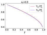
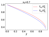
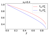
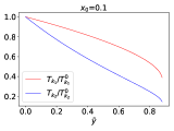
Figure 1: (Color online) The Kondo temperatures $T_{K1}$ and $T_{K2}$ of two magnetic impurities relative to their bare values, as function of the dimensionless RKKY coupling parameter between them, $\tilde{y}$, relative to its critical value for the homogenous system, for different bare Kondo temperature ratios $x_{0}=T^{0}_{K_{2}}/T^{0}_{K_{1}}=0.9,0.7,0.4,0.1$.

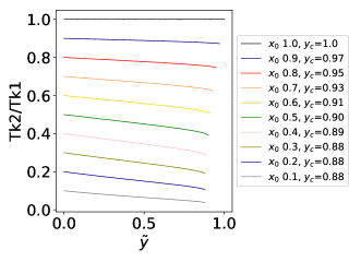
Figure 2: (Color online) The ratio of Kondo temperature of two magnetic impurities, $x=T_{K2}/T_{K1}$ as function of the dimensionless RKKY coupling parameter $\tilde{y}$, relative to its critical value for the homogenous system, for different bare Kondo temperature ratios $x_{0}=T^{0}_{K_{2}}/T^{0}_{K_{1}}=0.1,0.4,0.7,0.9$. The curves end at a critical value $\tilde{y}_{c}(x_{0})$, above which both Kondo impurities are quenched.

Moreover, the quenching of the Kondo screening by the RKKY coupling occurs already for smaller RKKY coupling, as seen in Fig. 2, the stronger the inhomogeneity and the smaller the ratio of the bare Kondo temperature $x_{0}$ is. For small $x_{0}$ the breakdown occurs at a critical value which converges to $y_{c}(x_{0}\ll 1)=0.88y_{c}$ of the critical RKKY coupling $y_{c}$ in the homogeneous system, Eq. (5), as confirmed in table 1. Thus, we find that inhomogeneity leaves the Kondo screening of the magnetic impurities more easily quenchable by RKKY coupling. In table 1 we notice that, while the larger of the two Kondo temperatures reaches at the critical coupling a value which is a little larger than the value it would read in a homogenous system $T_{K}(y_{c})=e^{-1}T^{0}_{K}\approx 0.368T^{0}_{K}$, the smaller Kondo temperature reaches a much lower Kondo temperature than it could reach in the homogenous system. As observed already above in Fig. 1 we also see that the smaller the initial ratio of Kondo temperatures $x_{0}$ is, the smaller the ratio of Kondo temperatures with coupling becomes, reaching for $x_{0}=0.1$ a ratio $x_{c}=0.038,$ just about one third of the initial ratio, confirming that the inequality between the Kondo temperatures becomes enhanced by the RKKY coupling. All that is seen in the three-dimensional plot Fig. 4 where the Kondo temperatures $T_{K1}$ and $T_{K2}$ relative to their bare values are plotted as function of bare Kondo temperature ratios $x_{0}$ and the dimensionless RKKY coupling parameters $\tilde{y}$, as well as in Fig. 5 where the ratio of the Kondo temperatures $x$ is plotted as function of $x_{0}$ and $\tilde{y}$. In table 2 we list the values of $T_{K1}$ and $T_{K2}$ and their ratio at the critical coupling for small $x_{0}.$ We see that the ratio of the Kondo temperatures $x$ decays rapidly with $x_{0}.$

$x_{0}$	$\tilde{y}_{c}$	$T_{K1}(\tilde{y}_{c})$/$T^{0}_{K1}$	$T_{K2}(\tilde{y}_{c})$/$T^{0}_{K2}$	$T_{K2}(\tilde{y}_{c})$/$T_{K1}(\tilde{y}_{c})$
1	1	0.368	0.368	1
0.9	0.97	0.407	0.395	0.872
0.8	0.95	0.396	0.370	0.746
0.7	0.93	0.398	0.355	0.634
0.6	0.91	0.414	0.350	0.517
0.5	0.90	0.398	0.312	0.392
0.4	0.89	0.400	0.286	0.286
0.3	0.88	0.414	0.264	0.191
0.2	0.88	0.399	0.210	0.105
0.1	0.88	0.391	0.147	0.038

Table 1: The Kondo temperatures at the respective critical coupling $\tilde{y}_{c}(x_{0})$ and their ratio as function of the ratio of bare couplings.

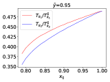
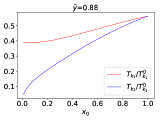
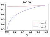
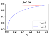
Figure 3: (Color online) The Kondo temperatures of two magnetic impurities, $T_{K1}$ and $T_{K2}$ relative to their bare values as function of bare Kondo temperature ratios $x_{0}$ for different dimensionless RKKY coupling parameters $\tilde{y}=0.95,0.88,0.5,0.3$.

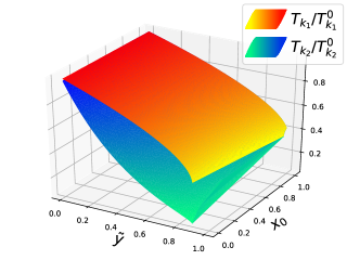
Figure 4: (Color online) Kondo temperatures of two magnetic impurities, $T_{K1}$ and $T_{K2}$ relative to their bare values as function of bare Kondo temperature ratios $x_{0}$ and the dimensionless RKKY coupling parameters $\tilde{y}$.

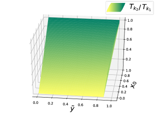
Figure 5: (Color online) Ratio of the Kondo temperatures of two magnetic impurities, $T_{K1}/T_{K2}$ as function of bare Kondo temperature ratios $x_{0}$ and the dimensionless RKKY coupling parameters $\tilde{y}$.

To confirm this anisotropic Kondo destruction, we consider the limit $x_{0}\rightarrow 0$, so that one of the two bare Kondo temperatures is vanishingly small. Then, Eq. (12) is reduced to

$$2\ln x_{1}+\frac{2\tilde{y_{1}}}{x_{1}\alpha e}+\mathcal{O}(x_{0}^{2})=0$$ (15)

and Eq. (13) to

$$2\ln x_{2}-\frac{4\tilde{y_{1}}}{x_{1}\alpha e}\ln(\frac{x_{0}x_{1}}{2x_{2}})+\mathcal{O}(x_{0}^{2})=0.$$ (16)

Solving Eq. (15), one finds $T_{K1}$ as a function of the effective RKKY interaction strength $\tilde{y_{1}}$. Inserting the maximum value of $\tilde{y_{1}}$ = $\alpha\sim 0.8813$, we obtain that $x_{1}$ remains to be finite and close to $1/e\sim 0.36$. Solving Eq. (16), we obtain $T_{K2}$ as a function of the ratio $x_{0}$ of bare Kondo temperatures. As a result, we have

$$x_{2}=\left(\frac{x_{0}x_{1}}{2}\right)^{\frac{\frac{2\tilde{y_{1}}}{x_{1}\alpha e}}{1+\frac{2\tilde{y_{1}}}{x_{1}\alpha e}}},$$ (17)

which decays rapidly as $x_{0}\rightarrow 0$, setting $x_{1}=1/e$ in accordance with the numerical solution tabled in table 2.

$\tilde{y_{1}}$	$x_{0}$	$T_{K1}$/$T^{0}_{K1}$	$T_{K2}$/$T^{0}_{K2}$	$T_{K2}$/$T_{K1}$
0.881	$10^{-3}$	0.372	0.0140	$3.76\times 10^{-2}x_{0}$
0.881	$10^{-4}$	0.371	0.00442	$1.19\times 10^{-2}x_{0}$
0.881	$10^{-5}$	0.366	0.00133	$3.63\times 10^{-3}x_{0}$
0.881	$10^{-6}$	0.367	0.000424	$1.16\times 10^{-3}x_{0}$
0.881	$10^{-7}$	0.375	0.000149	$3.97\times 10^{-4}x_{0}$

Table 2: Numerical solutions for Eqs. (12) and (13) in the $x_{0}\rightarrow 0$ limit.

III The Kondo effect in the system of randomly distributed magnetic impurities

Next, let us consider the generalisation of this theoretical framework to an electron system with a finite density of randomly distributed magnetic impurities, $n_{M}=N/Vol.$. As $N$ magnetic impurities are placed at random positions ${\bf r}_{i}$, $i=1,...,N$, they are coupled by random local exchange couplings $J^{0}_{i}$ to the conduction electrons with local density of states $\rho(E,{\bf r}_{i})$. Thereby, every magnetic moment placed at random positions has a different Kondo temperature, yielding a distribution of Kondo temperatures mott ; BhattFisher92 ; Lakner ; KondoDisorder ; Cornaglia2006 ; Mucciolo ; Micklitz05 ; Kats ; Slevin2019 . As the RKKY coupling is randomly distributed as well BhattFisher92 ; Lerner1993 ; HYLee2014 it remains an open problem to derive the quantum phase diagram of a disordered electron system with finite density of magnetic moments $n_{M}$. Using the definition of the RKKY couplings Eq. (3), we can now generalize the self-consistent renormalisation group equations Eq. (7) of the RKKY-coupled randomly distributed magnetic impurities. It is important to note that the local density of states $\rho({\bf r}_{i},E)$ does depend on energy $E$, so that at each RG scale $D$ the renormalisation of the local exchange coupling $J(\bm{r})$ depends on the local density of states at energy $E=\mu\pm D$, $\rho({\bf r}_{i},\mu\pm D)$, which may be different from the density of state at the chemical potential $\mu$, $\rho_{0i}=\rho({\bf r}_{i},\mu)$. Defining $g_{i}=J(\bm{r}_{i})\rho_{0i}$, we thereby find for the renormalisation of exchange couplings $g_{i}$

$$\frac{dg_{i}}{d\ln D}=-g_{i}^{2}\sum_{\alpha=\pm}\left(\frac{\rho(\mu+\alpha D,\bm{r}_{i})}{\rho_{0i}}-\frac{4J_{i}^{0}}{\pi\rho_{0i}}\sum_{j\neq i}J_{j}^{0}{\rm Im}[e^{i{\bf k}_{F}{\bf r}_{ij}}\chi_{c}({\bf r}_{ij},\mu+\alpha D)G^{R}_{c}({\bf r}_{ij},\mu+\alpha D)\chi_{f}({\bf r}_{j},\mu+\alpha D)]\right).$$ (18)

The first term on the right hand side corresponds to the 1-loop RG for the Kondo problem with energy dependent density of states suhl ; Zarand96 ; gapless . In the second term, $\chi_{f}({\bf r}_{j},E)$ is the full f-spin susceptibility of the magnetic impurity positioned at ${\bf r}_{j}$. $G^{R}_{c}({\bf r}_{ij},E)$ is the retarded conduction electron propagator from position ${\bf r}_{i}$ to ${\bf r}_{j}$ with ${\bf r}_{ij}={\bf r}_{i}-{\bf r}_{j}$. $\chi_{c}({\bf r}_{ij},E)$ is the conduction electron correlation function between positions ${\bf r}_{i}$ and ${\bf r}_{j}$.

At moderate magnetic impurity densities $n_{M}$, one may approximate $\chi_{f}({\bf r}_{j},E)$ by the expression for a single Kondo impurity which is known from Bethe-Ansatz solution bethe . This has been done in Ref. Nejati2017 , noting that only its real part contributes which is then given by ${\rm Re}\chi_{f}({\bf r}_{j},\mu+D)=W/(\pi T_{Kj}\sqrt{1+D^{2}/T_{Kj}^{2}})$, where $W$ is the Wilson ratio and $T_{Kj}$ is the Kondo temperature of the magnetic impurity at position ${\bf r}_{j}$.

In Ref. Nejati2017 it has been furthermore assumed that all conduction electron properties, the local density of states, the propagator $G^{R}_{c}({\bf r}_{ij},E)$ and the correlation function $\chi_{c}({\bf r}_{ij},E)$ depend only weakly on energy, and therefore can be replaced by its value at the chemical potential $\mu$. Let us therefore at first follow this assumption, although it is well known that the energy dependence can change the Kondo renormalisation gapless and modify the distribution of Kondo temperatures in disordered systems substantially Mucciolo ; Zhuravlev2007 ; Kats ; Slevin2019 . Introducing furthermore the continuum representation, by denoting $g(\bm{r})=g_{i}$ and $\bm{r}=\bm{r}_{i}$, we can rewrite the RG equation as

$$\frac{dg(\bm{r})}{d\ln D}=-2g(\bm{r})^{2}\left(1-g_{0}(\bm{r})D_{0}\int d^{3}\bm{r}^{\prime}g_{0}(\bm{r^{\prime}})\frac{y(\bm{r}-\bm{r}^{\prime})}{T_{K}(\bm{r}^{\prime})}\frac{1}{\sqrt{1+(D/T_{K}(\bm{r}^{\prime}))^{2}}}\right).$$ (19)

where we introduced the function $y(\bm{r}-\bm{r}^{\prime})$ defined by

$$y(\bm{r}-\bm{r}^{\prime})=-\frac{8W}{\pi^{2}\rho_{0}(\bm{r})}{\rm Im}\sum_{j\neq i}\frac{1}{\rho_{0}(\bm{r_{j}})}\delta({{\bf r}^{\prime}-{\bf r}_{j}})e^{i{\bf k}_{F}({\bf r}-{\bf r}_{j})}G^{R}_{c}({\bf r}-{\bf r}_{j},\mu)\chi_{c}({\bf r}-{\bf r}_{j},\mu).$$ (20)

As a result, we obtain the self-consistent equation with RKKY interactions in the dilute limit of randomly distributed magnetic impurities,

$$-\frac{1}{g_{0}(\bm{r})}=2\ln\Big{(}\frac{T_{K}(\bm{r})}{D_{0}}\Big{)}-g_{0}(\bm{r})D_{0}\int d^{3}\bm{r}^{\prime}g_{0}(\bm{r}^{\prime})\frac{y(\bm{r}-\bm{r}^{\prime})}{T_{K}(\bm{r}^{\prime})}\ln\Big{(}\frac{\sqrt{1+[T_{K}(\bm{r})/T_{K}(\bm{r}^{\prime})]^{2}}-1}{\sqrt{1+[T_{K}(\bm{r})/T_{K}(\bm{r}^{\prime})]^{2}}+1}\Big{)}.$$ (21)

Solving this integral equation, we can derive the position dependent Kondo temperatures for a given configuration of RKKY interactions. From the distribution of the local couplings $g_{0}(\bm{r})$ which originates from the random positions of doped magnetic impurities, the long range function $y(\bm{r}-\bm{r}^{\prime})$, together with the random distribution of electronic properties like the local density of states, we can thus derive from Eq. (21) the distribution function of Kondo temperatures $T_{K}$. We note that it has been found before that the random distribution of RKKY-coupling is mainly due to the distribution of local couplings $g_{0}(\bm{r})$ HYLee2014 , so that the distribution originates mainly from the local couplings $g_{0}(\bm{r})$, while the function $y(\bm{r}-\bm{r}^{\prime})$ is not strongly modified by the disorder.

When the RKKY interaction is neglected it has been derived before that the Kondo temperature has a bimodal distribution with a low $T_{K}$ peak and a peak close to the Kondo temperature of the clean systems KondoDisorder ; Cornaglia2006 ; Mucciolo ; Kats ; Slevin2019 . The low $T_{K}$-peak was found to become more pronounced for stronger disorder and converges to a universal power law tail at the Anderson metal-insulator transition, where the power exponent depends only on the multifractality parameter $\alpha_{0}$ Kats ; Slevin2019 . It remains to find out, whether the relevance of inequalities found for two magnetic impurities with RKKY-interaction above, where we found that the lower Kondo temperature is suppressed more strongly, results in a further enhancement of the low Kondo temperature peak in its distribution and thereby of the low temperature magnetic susceptibility. This question can be resolved by the solution of Eq. (21), which we leave for further study.

- (1) S. Doniach, Physica B+C 91, 231 (1977).
- (2) A. Nejati, K. Ballmann, J. Kroha, Phys. Rev. Lett. 118, 117204 (2017).
- (3) H. von Löhneysen, Ann. Phys. (Berlin) 523, 599 (2011).
- (4) E. Miranda and V. Dobrosavljevic, Reports on Progress in Physics 68, 2337 (2005).
- (5) M. A. Ruderman and C. Kittel, Phys. Rev. 96, 99 (1954); T. Kasuya, Prog. Theor. Phys. 16, 45 (1956); K. Yosida, Phys. Rev. 106, 893 (1957).
- (6) P. W. Anderson, Phys. Rev. 109, 1492 (1958); Nobel Lectures in Phys. 1980, 376 (1977).
- (7) N. Mott, Rev. Mod. Phys. 40, 677 (1968); N. F. Mott, J. Phys. Colloques 37, 301 (1976).
- (8) R. N. Bhatt and D. S. Fisher, Phys. Rev. Lett. 68, 3072 (1992).
- (9) P. B. Chakraborty, K. Byczuk, and D. Vollhardt, Phys. Rev. B 84, 035121 (2011).
- (10) M. Ulmke and R. T. Scalettar, Phys. Rev. B 55, 4149 (1997).
- (11) M. E. Pezzoli and F. Becca, Phys. Rev. B 81, 075106 (2010).
- (12) K. Byczuk, W. Hofstetter, U. Yu, and D. Vollhardt, Eur. Phys. J. Spec. Top 180, 135 (2009).
- (13) M. Ulmke, V. Janis, and D. Vollhardt, Phys. Rev. B 51, 10411 (1995).
- (14) M. C. O. Aguiar, V. Dobrosavljevic, E. Abrahams, and G. Kotliar, Phys. Rev. B 73, 115117 (2006).
- (15) M. C. O. Aguiar, V. Dobrosavljevic, E. Abrahams, and G. Kotliar, Phys. Rev. Lett. 102, 156402 (2009).
- (16) D.Tanaskovic,V.Dobrosavljevic, E.Abrahams,and G. Kotliar, Phys. Rev. Lett. 91, 066603 (2003).
- (17) M. C. O. Aguiar and V. Dobrosavljevic, Phys. Rev. Lett. 110, 066401 (2013).
- (18) K. Byczuk, W. Hofstetter, and D. Vollhardt, Phys. Rev. Lett. 94, 056404 (2005).
- (19) M. Milovanović, S. Sachdev, and R. N. Bhatt, Phys. Rev. Lett. 63, 82 (1989).
- (20) S. Sachdev, Phil. Trans. R. Soc. A 356, 173 (1998).
- (21) M. A. Tusch and D. E. Logan, Phys. Rev. B 48, 14843 (1993).
- (22) S. Sen, N. S. Vidhyadhiraja, M. Jarrell, arXiv:1708.04086v1 (2017).
- (23) C. E. Ekuma, H. Terletska, K.-M. Tam, Z.-Y. Meng, J. Moreno, et al., Phys. Rev. B 89, 081107 (2014).
- (24) H. Y. Lee, S. Kettemann, Phys. Rev. B 89, 165109 (2014).
- (25) A. M. Tsvelick and P. B. Wiegmann, Adv. Phys. 32, 453 (1983); N. Andrei, K. Furuya, and J. H. Lowenstein, Rev. Mod. Phys. 55, 331 (1983).
- (26) M. Lakner, H. v. Löhneysen, A. Langenfeld, and P. Wölfle Phys. Rev. B 50, 17064 (1994); A. Langenfeld and P Wölfle, Ann. Phys. 4, 43 (1995).
- (27) V. Dobrosavljevic, T. R. Kirkpatrick, and G. Kotliar, Phys. Rev. Lett. 69, 1113 (1992); E. Miranda, V. Dobrosavljevic, and G. Kotliar, ibid. 78, 290 (1997).
- (28) P. S. Cornaglia, D. R. Grempel, and C. A. Balseiro, Phys. Rev. Lett. 96, 117209 (2006).
- (29) S. Kettemann and E. R. Mucciolo, JETP Lett. 83, 240 (2006) [Pis’ma v ZhETF 83,284 (2006)]; Phys. Rev. B 75, 184407 (2007).
- (30) T. Micklitz, A. Altland, T. A. Costi, and A. Rosch, Phys. Rev. Lett. 96, 226601 (2006).
- (31) S. Kettemann, E. R. Mucciolo, and I. Varga, Phys. Rev. Lett. 103, 126401 (2009); S. Kettemann, E. R. Mucciolo, I. Varga, K. Slevin, Phys. Rev. B 85, 115112 (2012).
- (32) K. Slevin, S. Kettemann and T. Ohtsuki, Eur. Phys. J. B 92, 281 (2019).
- (33) V. Lerner, Phys. Rev. B 48, 9462 (1993).
- (34) Y. Nagaoka, Phys. Rev. 138, 1112 (1965); H. Suhl, Phys. Rev. A 138, 515 (1965).
- (35) G. Zarand and L. Udvardi, Phys. Rev. B 54, 7606 (1996).
- (36) D. Withoff and E. Fradkin, Phys. Rev. Lett. 64, 1835 (1990); K. Ingersent, Phys. Rev. B 54, 11936(1996).
- (37) A. Zhuravlev, I. Zharekeshev, E. Gorelov, A. I. Lichtenstein, E. R. Mucciolo, and S. Kettemann, Phys. Rev. Lett. 99, 247202 (2007).