Run-and-tumble motion: field theory and entropy production

Abstract

Run-and-tumble motion is an example of active motility where particles move at constant speed and change direction at random times. In this work we study run-and-tumble motion with diffusion in a harmonic potential in one dimension via a path integral approach. We derive a Doi-Peliti field theory and use it to calculate the entropy production and other observables in closed form. All our results are exact.

1 Introduction

Active matter encompasses reaction-diffusion systems out of equilibrium whose components are subject to local non-thermal forces [1]. There is a plethora of interesting patterns and phenomenology in this broad class of systems. Some fascinating examples are active nematics [2, 3, 4], active emulsions [5], and active motility [6, 7], amongst many others. Active matter has become a research focus in statistical mechanics over recent years, as it addresses fundamental questions on the physics of non-equilibrium systems, but also as a quantitative approach to biological physics and the path to designing an autonomous microbiological engine [8, 9, 10, 11].

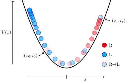
In this paper we study a model of active motility known as run and tumble (RnT) that has been used to describe bacterial swimming patterns such as that of Escherichia coli and Salmonella [12, 13]. A particle undergoing run-and-tumble motion moves in a sequence of runs at constant self-propulsion speed $w$ interrupted by sudden changes (tumbles) in its orientation that happen at Poissonian rate $\alpha$, [14, 15, 16, 17, 18, 19, 20, 21]. This motion pattern is ballistic at the microscopic scale and diffusive at the large scale with effective diffusion constant $D_{\text{eff}}=w^{2}/\alpha$ [22, 23, 24, 25, 20, 12, 26, 27]. We study a run-and-tumble particle subject to thermal noise confined in a harmonic potential $V(x)=kx^{2}/2$, see figure 1.

We follow a path integral approach [15] whereby we derive a perturbative field theory in the Doi-Peliti framework [28] and use it to calculate a number of observables in closed form, with an emphasis on the entropy production [29]. Despite our approach being perturbative, all our results are exact. The presence of the external potential presents technical challenges in the derivation of the field theory that resemble those encountered in other contexts such as the quantum harmonic oscillator [30, 31, 32]. We use a combination of the Fourier transform and Hermite polynomials to parametrise the fields as to diagonalise the action functional.

We regard the Doi-Peliti framework as a method to solve a master equation, or a Fokker-Planck equation. It therefore crucially retains the microscopic dynamics of the system and captures the particle entity. For this reason, the Doi-Peliti framework provides a solid route to calculate the entropy production and, most importantly, proves itself to be an effective tool to study active particle systems. In this paper, we illustrate this point by studying RnT motion.

The contents of this paper are organised as follows: in Sec. 2, we derive a field theory for an RnT particle in a harmonic potential; in Sec. 3 we use this field theory to calculate the entropy production; and in Sec. 4 we discuss our results. In the appendix, we have included other relevant observables: mean square displacement (C), two-point correlation functions (E and F), expected velocity (D), and stationary distribution (G).

Figure 1: Trajectory snapshots of an RnT particle in a harmonic potential $V(x)$ (solid line). Initially, the particle at $(x_{0},t_{0})$ is right-moving with positive velocity $w$ (red circles), until it tumbles at $(x_{1},t_{1})$ and becomes left-moving with negative velocity $-w$ (blue circles).

2 Field theory of run-and-tumble motion with diffusion in a harmonic potential

In one dimension, we can think of run-and-tumble motion as the interaction between right- and left-moving particles that transmute into one another at Poissonian rate $\alpha/2$, see figure 1. The Langevin equations of each species are

$$\dot{x}_{\phi}=-\partial_{x}V(x)+w+\eta(t)$$ (1)

for right-moving particles and

$$\dot{x}_{\psi}=-\partial_{x}V(x)-w+\eta(t)$$ (2)

for left-moving particles, where $\eta$ is a Gaussian white noise with mean $\left\langle{\eta(t)}\right\rangle=0$ and correlation function $\left\langle{\eta(t)\eta(t^{\prime})}\right\rangle=2D\delta(t-t^{\prime})$, with diffusion constant $D$. The corresponding Fokker-Plank equations are coupled due to the transmutation between species through a gain and loss terms,

$$\partial_{t}P_{\phi}=-\partial_{x}\left[(-kx+w)P_{\phi}\right]+D\partial_{x}^{2}P_{\phi}+\frac{\alpha}{2}(P_{\psi}-P_{\phi})\,,$$ (3a)

$$\partial_{t}P_{\psi}=-\partial_{x}\left[(-kx-w)P_{\psi}\right]+D\partial_{x}^{2}P_{\psi}+\frac{\alpha}{2}(P_{\phi}-P_{\psi})\,,$$ (3b)

where $P_{\phi}(x,t)$ and $P_{\psi}(x,t)$ are the probability densities of a right- and a left-moving particle respectively, as a function of position $x$ and time $t$. It follows that the action functional [39] of this process is

$$\mathcal{A}=\int\mathchoice{\!\text{d}x\,}{\!\text{d}x\,}{\!\text{d}x\,}{\!\text{d}x\,}\mathchoice{\!\text{d}t\,}{\!\text{d}t\,}{\!\text{d}t\,}{\!\text{d}t\,}\big{\{}\widetilde{\phi}\left(\partial_{t}\phi+\partial_{x}\left[(-kx+w)\phi\right]-D\partial_{x}^{2}\phi\right)$$

$$\qquad+\widetilde{\psi}\left(\partial_{t}\psi+\partial_{x}\left[(-kx-w)\psi\right]-D\partial_{x}^{2}\psi\right)+\frac{\alpha}{2}(\widetilde{\phi}-\widetilde{\psi})(\phi-\psi)\big{\}}\,$$ (4)

where $\phi$ is the annihilation field of right-moving particles; $\widetilde{\phi}$ is the Doi-shifted [33] creation field $\phi^{\dagger}=\widetilde{\phi}+1$ of right-moving particles; $\psi$ is the annihilation field of left-moving particles; and $\widetilde{\psi}$ is the Doi-shifted creation field $\psi^{\dagger}=\widetilde{\psi}+1$ of left-moving particles. The action functional (4) allows the calculation of an observable $\bullet$ via the path integral

$$\left\langle{\bullet}\right\rangle=\int\mathcal{D}[\phi,\widetilde{\phi},\psi,\widetilde{\psi}]\bullet\mathchoice{e^{-\mathcal{A}([\phi,\widetilde{\phi},\psi,\widetilde{\psi}])}}{\operatorname{exp}\!\left(-\mathcal{A}([\phi,\widetilde{\phi},\psi,\widetilde{\psi}])\right)}{\operatorname{exp}\!\left(-\mathcal{A}([\phi,\widetilde{\phi},\psi,\widetilde{\psi}])\right)}{\operatorname{exp}\!\left(-\mathcal{A}([\phi,\widetilde{\phi},\psi,\widetilde{\psi}])\right)}\,.$$ (5)

The action in Equation (4) contains only bilinear terms, where the only interaction between species is due to transmutation. This action does not have any non-linear couplings. Motivated by the matrix representation of the action (4), we refer to any terms involving $\widetilde{\phi}\phi$ or $\widetilde{\psi}\psi$ as diagonal terms, and to the terms $\widetilde{\phi}\psi$ and $\widetilde{\psi}\phi$ as off-diagonal terms. The diagonal terms in (4) are semi-local due to the derivatives in space and time, which need to be made local in order to carry out the Gaussian (path) integral. This is usually achieved by expressing the fields in Fourier space. In this case, however, Fourier-transforming (4) yields the action local in the frequency $\omega$ but not in reciprocate position $x$. Due to the diagonal terms $-k\widetilde{\phi}\partial_{x}(x\phi)$ $-k\widetilde{\psi}\partial_{x}(x\psi)$, the action remains semi-local after Fourier-transforming.

Instead, we first parametrise the action by the density field $\rho=(\phi+\psi)/\sqrt{2}$ and the polarity field $\nu=(\phi-\psi)/\sqrt{2}$, also called chirality [34], with the analogous transformation for the conjugate fields. This change of variables is useful in other contexts and is known under other names, such as the Keldysh rotation [35]. In our case, the advantage is that the action remains invariant under the transformation $\rho\leftrightarrow\nu$, $\widetilde{\rho}\leftrightarrow\widetilde{\nu}$, except for the mass term $\alpha\widetilde{\nu}\nu$,

$$\mathcal{A}=\int\mathchoice{\!\text{d}x\,}{\!\text{d}x\,}{\!\text{d}x\,}{\!\text{d}x\,}\mathchoice{\!\text{d}\mkern-6.0mu\mathchar 22\relax\omega\,}{\!\text{d}\mkern-6.0mu\mathchar 22\relax\omega\,}{\!\text{d}\mkern-6.0mu\mathchar 22\relax\omega\,}{\!\text{d}\mkern-6.0mu\mathchar 22\relax\omega\,}\big{\{}-\mathring{\imath}\omega\widetilde{\rho}\rho-k\widetilde{\rho}\partial_{x}(x\rho)-D\widetilde{\rho}\partial_{x}^{2}\rho$$

$$\qquad-\mathring{\imath}\omega\widetilde{\nu}\nu-k\widetilde{\nu}\partial_{x}(x\nu)-D\widetilde{\nu}\partial_{x}^{2}\nu+\alpha\widetilde{\nu}\nu+w\widetilde{\rho}\partial_{x}\nu+w\widetilde{\nu}\partial_{x}\rho\big{\}}\,.$$ (6)

We then use the solution to the eigenvalue problem $\mathcal{L}[u(x)]=\lambda u(x)$, with

$$\mathcal{L}[u(x)]=\partial_{x}^{2}u(x)+\partial_{x}(x\,u(x))/L^{2}\ ,$$ (7)

$L=\sqrt{D/k}$ and $\lambda\in\mathbb{R}$, where the differential operator follows from the diagonal terms in (6). By using the fields $\rho$ and $\nu$, instead of the original $\phi$ and $\psi$, we have the same differential operator $\mathcal{L}$ acting on both $\rho$ and $\nu$.

The solution to this eigenvalue problem is the set of Hermite functions

$$u_{n}(x)=\mathchoice{e^{-\frac{x^{2}}{2L^{2}}}}{\operatorname{exp}\!\left(-\frac{x^{2}}{2L^{2}}\right)}{\operatorname{exp}\!\left(-\frac{x^{2}}{2L^{2}}\right)}{\operatorname{exp}\!\left(-\frac{x^{2}}{2L^{2}}\right)}\,H_{n}\left(\frac{x}{L}\right)\,,$$ (8)

with eigenvalue $\lambda_{n}=-{n}/{L^{2}}$, where $H_{n}\left(x\right)$ is the $n$-th Hermite polynomial, see A [36, 37, 30]. Defining the set of functions

$$\widetilde{u}_{n}(x)=\frac{1}{\sqrt{{2\pi}}\,n!}{H_{n}\left(\frac{x}{L}\right)}\,,$$ (9)

the orthogonality relation between $u_{n}(x)$ and $\widetilde{u}_{m}(x)$ follows from the orthogonality of Hermite polynomials in Equation (22an),

$$\int_{-\infty}^{\infty}\mathchoice{\!\text{d}x\,}{\!\text{d}x\,}{\!\text{d}x\,}{\!\text{d}x\,}u_{n}(x)\widetilde{u}_{m}(x)=L\,\delta_{n,m}\,,$$ (10)

where $\delta_{n,m}$ is the Kronecker $\delta$. We can now use $u_{n}$ and $\widetilde{u}_{m}$ as basis for the fields $\rho$, $\widetilde{\rho}$, $\nu$ and $\widetilde{\nu}$,

$$\mathord{\mathop{\rho}\limits^{\scriptscriptstyle(\sim)}}(x,t)=\int\mathchoice{\!\text{d}\mkern-6.0mu\mathchar 22\relax\omega\,}{\!\text{d}\mkern-6.0mu\mathchar 22\relax\omega\,}{\!\text{d}\mkern-6.0mu\mathchar 22\relax\omega\,}{\!\text{d}\mkern-6.0mu\mathchar 22\relax\omega\,}\mathchoice{e^{-\mathring{\imath}\omega t}}{\operatorname{exp}\!\left(-\mathring{\imath}\omega t\right)}{\operatorname{exp}\!\left(-\mathring{\imath}\omega t\right)}{\operatorname{exp}\!\left(-\mathring{\imath}\omega t\right)}\frac{1}{L}\sum_{n}\mathord{\mathop{\rho}\limits^{\scriptscriptstyle(\sim)}}_{n}(\omega)\mathord{\mathop{u}\limits^{\scriptscriptstyle(\sim)}}_{n}(x)\,,$$ (11a)

$$\mathord{\mathop{\nu}\limits^{\scriptscriptstyle(\sim)}}(x,t)=\int\mathchoice{\!\text{d}\mkern-6.0mu\mathchar 22\relax\omega\,}{\!\text{d}\mkern-6.0mu\mathchar 22\relax\omega\,}{\!\text{d}\mkern-6.0mu\mathchar 22\relax\omega\,}{\!\text{d}\mkern-6.0mu\mathchar 22\relax\omega\,}\mathchoice{e^{-\mathring{\imath}\omega t}}{\operatorname{exp}\!\left(-\mathring{\imath}\omega t\right)}{\operatorname{exp}\!\left(-\mathring{\imath}\omega t\right)}{\operatorname{exp}\!\left(-\mathring{\imath}\omega t\right)}\frac{1}{L}\sum_{n}\mathord{\mathop{\nu}\limits^{\scriptscriptstyle(\sim)}}_{n}(\omega)\mathord{\mathop{u}\limits^{\scriptscriptstyle(\sim)}}_{n}(x)\,.$$ (11b)

Using the representation (11) and the orthogonality relation (10) in the action $\mathcal{A}=\mathcal{A}_{0}+\mathcal{A}_{1}$ in (6), we have

$$\mathcal{A}_{0}=\frac{1}{L^{2}}\sum_{n,m}L\delta_{n,m}\int\mathchoice{\!\text{d}\mkern-6.0mu\mathchar 22\relax\omega\,}{\!\text{d}\mkern-6.0mu\mathchar 22\relax\omega\,}{\!\text{d}\mkern-6.0mu\mathchar 22\relax\omega\,}{\!\text{d}\mkern-6.0mu\mathchar 22\relax\omega\,}\mathchoice{\!\text{d}\mkern-6.0mu\mathchar 22\relax\omega^{\prime}\,}{\!\text{d}\mkern-6.0mu\mathchar 22\relax\omega^{\prime}\,}{\!\text{d}\mkern-6.0mu\mathchar 22\relax\omega^{\prime}\,}{\!\text{d}\mkern-6.0mu\mathchar 22\relax\omega^{\prime}\,}\delta\mkern-8.0mu\mathchar 22\relax(\omega+\omega^{\prime})$$

$$\qquad\times\big{[}\left(-\mathring{\imath}\omega+kn\right)\tilde{\rho}_{n}(\omega^{\prime}){\rho}_{m}(\omega)+\left(-\mathring{\imath}\omega+kn+\alpha\right)\tilde{\nu}_{n}(\omega^{\prime}){\nu}_{m}(\omega)\big{]}\,,$$ (12a)

$$\mathcal{A}_{1}=-\frac{w}{L}\frac{1}{L^{2}}\sum_{n,m}L\delta_{n-1,m}\int\mathchoice{\!\text{d}\mkern-6.0mu\mathchar 22\relax\omega\,}{\!\text{d}\mkern-6.0mu\mathchar 22\relax\omega\,}{\!\text{d}\mkern-6.0mu\mathchar 22\relax\omega\,}{\!\text{d}\mkern-6.0mu\mathchar 22\relax\omega\,}\mathchoice{\!\text{d}\mkern-6.0mu\mathchar 22\relax\omega^{\prime}\,}{\!\text{d}\mkern-6.0mu\mathchar 22\relax\omega^{\prime}\,}{\!\text{d}\mkern-6.0mu\mathchar 22\relax\omega^{\prime}\,}{\!\text{d}\mkern-6.0mu\mathchar 22\relax\omega^{\prime}\,}\delta\mkern-8.0mu\mathchar 22\relax(\omega+\omega^{\prime})\big{[}\tilde{\rho}_{n}(\omega^{\prime}){\nu}_{m}(\omega)+\tilde{\nu}_{n}(\omega^{\prime}){\rho}_{m}(\omega)\big{]}\,,$$ (12b)

where $\mathcal{A}_{0}$ contains the local, diagonal terms and $\mathcal{A}_{1}$ contains the off-diagonal terms, which are non-local due to $\delta_{n-1,m}$. We can then regard $\mathcal{A}_{0}$ as the Gaussian model and $\mathcal{A}_{1}$ as a perturbation about it.

The Gaussian model corresponds to Ornstein-Uhlenbeck particles where one species has decay rate $\alpha$. Defining an observable $\bullet$ in the Gaussian model as

$$\left\langle{\bullet}\right\rangle_{0}=\int\mathcal{D}[\rho,\widetilde{\rho},\nu,\widetilde{\nu}]\bullet\mathchoice{e^{-\mathcal{A}_{0}([\rho,\widetilde{\rho},\nu,\widetilde{\nu}])}}{\operatorname{exp}\!\left(-\mathcal{A}_{0}([\rho,\widetilde{\rho},\nu,\widetilde{\nu}])\right)}{\operatorname{exp}\!\left(-\mathcal{A}_{0}([\rho,\widetilde{\rho},\nu,\widetilde{\nu}])\right)}{\operatorname{exp}\!\left(-\mathcal{A}_{0}([\rho,\widetilde{\rho},\nu,\widetilde{\nu}])\right)}\,,$$ (13)

from (5) it follows that the perturbation expansion of the observable in the full model, the RnT particle, is

$$\left\langle{\bullet}\right\rangle=\left\langle{\bullet\mathchoice{e^{-\mathcal{A}_{1}}}{\operatorname{exp}\!\left(-\mathcal{A}_{1}\right)}{\operatorname{exp}\!\left(-\mathcal{A}_{1}\right)}{\operatorname{exp}\!\left(-\mathcal{A}_{1}\right)}}\right\rangle_{0}=\sum_{N=0}^{\infty}\frac{1}{N!}\left\langle{\bullet(-\mathcal{A}_{1})^{N}}\right\rangle_{0}\,.$$ (14)

By performing the Gaussian path integral [38] in (13), the bare propagators read

$$\leavevmode\hbox to73.62pt{\vbox to17.37pt{\pgfpicture\makeatletter\hbox{\hskip 35.93947pt\lower-0.5pt\hbox to0.0pt{\pgfsys@beginscope\pgfsys@invoke{ }\definecolor{pgfstrokecolor}{rgb}{0,0,0}\pgfsys@color@rgb@stroke{0}{0}{0}\pgfsys@invoke{ }\pgfsys@color@rgb@fill{0}{0}{0}\pgfsys@invoke{ }\pgfsys@setlinewidth{0.4pt}\pgfsys@invoke{ }\nullfont\pgfsys@beginscope\pgfsys@invoke{ }\pgfsys@invoke{\lxSVG@closescope }\pgfsys@endscope\hbox to0.0pt{\pgfsys@beginscope\pgfsys@invoke{ }{ {{}}\hbox{\hbox{{\pgfsys@beginscope\pgfsys@invoke{ }{{}{}{{ {}{}}}{ {}{}} {{}{{}}}{{}{}}{}{{}{}} { }{{{{}}\pgfsys@beginscope\pgfsys@invoke{ }\pgfsys@transformcm{1.0}{0.0}{0.0}{1.0}{8.33218pt}{6.033pt}\pgfsys@invoke{ }\hbox{{\definecolor{pgfstrokecolor}{rgb}{0,0,0}\pgfsys@color@rgb@stroke{0}{0}{0}\pgfsys@invoke{ }\pgfsys@color@rgb@fill{0}{0}{0}\pgfsys@invoke{ }\hbox{{$\tilde{\rho}_{m}(\omega^{\prime})$}} }}\pgfsys@invoke{\lxSVG@closescope }\pgfsys@endscope}}} \pgfsys@invoke{\lxSVG@closescope }\pgfsys@endscope}}} {{}}\hbox{\hbox{{\pgfsys@beginscope\pgfsys@invoke{ }{{}{}{{ {}{}}}{ {}{}} {{}{{}}}{{}{}}{}{{}{}} { }{{{{}}\pgfsys@beginscope\pgfsys@invoke{ }\pgfsys@transformcm{1.0}{0.0}{0.0}{1.0}{-32.60646pt}{6.033pt}\pgfsys@invoke{ }\hbox{{\definecolor{pgfstrokecolor}{rgb}{0,0,0}\pgfsys@color@rgb@stroke{0}{0}{0}\pgfsys@invoke{ }\pgfsys@color@rgb@fill{0}{0}{0}\pgfsys@invoke{ }\hbox{{${\rho}_{n}(\omega)$}} }}\pgfsys@invoke{\lxSVG@closescope }\pgfsys@endscope}}} \pgfsys@invoke{\lxSVG@closescope }\pgfsys@endscope}}} {}{{}}{} {}{}\pgfsys@beginscope\pgfsys@invoke{ }\pgfsys@setlinewidth{1.0pt}\pgfsys@invoke{ }\definecolor[named]{pgfstrokecolor}{rgb}{0,0,0}\pgfsys@color@gray@stroke{0}\pgfsys@invoke{ }{}\pgfsys@moveto{21.33957pt}{0.0pt}\pgfsys@lineto{-21.33957pt}{0.0pt}\pgfsys@stroke\pgfsys@invoke{ } \pgfsys@invoke{\lxSVG@closescope }\pgfsys@endscope} \pgfsys@invoke{\lxSVG@closescope }\pgfsys@endscope{}{}{}\hss}\pgfsys@discardpath\pgfsys@invoke{\lxSVG@closescope }\pgfsys@endscope\hss}}\lxSVG@closescope\endpgfpicture}}\,\hat{=}\langle{\rho_{n}(\omega)\tilde{\rho}_{m}(\omega^{\prime})}\rangle_{0}=\frac{L\delta_{n,m}\delta\mkern-8.0mu\mathchar 22\relax(\omega+\omega^{\prime})}{-\mathring{\imath}\omega+kn+r}\,, \tilde{\rho}_{m}(\omega^{\prime}) {\rho}_{n}(\omega) \tilde{\rho}_{m}(\omega^{\prime}) {\rho}_{n}(\omega)$$ (15a)

$$\leavevmode\hbox to73.5pt{\vbox to18.79pt{\pgfpicture\makeatletter\hbox{\hskip 35.82431pt\lower-1.92264pt\hbox to0.0pt{\pgfsys@beginscope\pgfsys@invoke{ }\definecolor{pgfstrokecolor}{rgb}{0,0,0}\pgfsys@color@rgb@stroke{0}{0}{0}\pgfsys@invoke{ }\pgfsys@color@rgb@fill{0}{0}{0}\pgfsys@invoke{ }\pgfsys@setlinewidth{0.4pt}\pgfsys@invoke{ }\nullfont\pgfsys@beginscope\pgfsys@invoke{ }\pgfsys@invoke{\lxSVG@closescope }\pgfsys@endscope\hbox to0.0pt{\pgfsys@beginscope\pgfsys@invoke{ }{ {{}}\hbox{\hbox{{\pgfsys@beginscope\pgfsys@invoke{ }{{}{}{{ {}{}}}{ {}{}} {{}{{}}}{{}{}}{}{{}{}} { }{{{{}}\pgfsys@beginscope\pgfsys@invoke{ }\pgfsys@transformcm{1.0}{0.0}{0.0}{1.0}{8.33218pt}{6.033pt}\pgfsys@invoke{ }\hbox{{\definecolor{pgfstrokecolor}{rgb}{0,0,0}\pgfsys@color@rgb@stroke{0}{0}{0}\pgfsys@invoke{ }\pgfsys@color@rgb@fill{0}{0}{0}\pgfsys@invoke{ }\hbox{{$\tilde{\nu}_{m}(\omega^{\prime})$}} }}\pgfsys@invoke{\lxSVG@closescope }\pgfsys@endscope}}} \pgfsys@invoke{\lxSVG@closescope }\pgfsys@endscope}}} {{}}\hbox{\hbox{{\pgfsys@beginscope\pgfsys@invoke{ }{{}{}{{ {}{}}}{ {}{}} {{}{{}}}{{}{}}{}{{}{}} { }{{{{}}\pgfsys@beginscope\pgfsys@invoke{ }\pgfsys@transformcm{1.0}{0.0}{0.0}{1.0}{-32.4913pt}{6.033pt}\pgfsys@invoke{ }\hbox{{\definecolor{pgfstrokecolor}{rgb}{0,0,0}\pgfsys@color@rgb@stroke{0}{0}{0}\pgfsys@invoke{ }\pgfsys@color@rgb@fill{0}{0}{0}\pgfsys@invoke{ }\hbox{{${\nu}_{n}(\omega)$}} }}\pgfsys@invoke{\lxSVG@closescope }\pgfsys@endscope}}} \pgfsys@invoke{\lxSVG@closescope }\pgfsys@endscope}}} {}{{}}{} {}{} {}{{}{}}{}{}{}{{}}{{}}{{}{}}{{}{}}{{{{}{}{{}} }}{{}} {}{}{} }{{{{}{}{{}} }}{{}} {{}{}{}{}} {{}{}{}{}} }{{{{}{}{{}} }}{{}} {{}{}{}{}} {{}{}{}{}} }{{{{}{}{{}} }}{{}} {{}{}{}{}} {{}{}{}{}} }{{{{}{}{{}} }}{{}} {{}{}{}{}} {{}{}{}{}} }{{{{}{}{{}} }}{{}} {{}{}{}{}} {{}{}{}{}} }{{{{}{}{{}} }}{{}} {{}{}{}{}} {{}{}{}{}} }{{{{}{}{{}} }}{{}} {{}{}{}{}} {{}{}{}{}} }{{{{}{}{{}} }}{{}} {{}{}{}{}} {{}{}{}{}} }{{{{}{}{{}} }}{{}} {{}{}{}{}} {{}{}{}{}} }{{{{}{}{{}} }}{{}} {{}{}{}{}} {{}{}{}{}} }{{{{}{}{{}} }}{{}} {{}{}{}{}} {{}{}{}{}} }{{{{}{}{{}} }}{{}} {{}{}{}{}} {{}{}{}{}} }{{{{}{}{{}} }}{{}} {{}{}{}{}} {{}{}{}{}} }{{{{}{}{{}} }}{{}} {{}{}{}{}} {{}{}{}{}} }{{{{}{}{{}} }}{{}} {{}{}{}{}} {{}{}{}{}} }{{{{}{}{{}} }}{{}} {{}} } \pgfsys@beginscope\pgfsys@invoke{ }\pgfsys@setlinewidth{1.0pt}\pgfsys@invoke{ }\definecolor[named]{pgfstrokecolor}{rgb}{0,0,0}\pgfsys@color@gray@stroke{0}\pgfsys@invoke{ }{}\pgfsys@moveto{21.33957pt}{0.0pt}\pgfsys@curveto{20.71457pt}{0.0pt}{20.40207pt}{-1.42264pt}{19.77707pt}{-1.42264pt}\pgfsys@curveto{19.32457pt}{-1.42264pt}{18.93459pt}{-0.7284pt}{18.52707pt}{0.0pt}\pgfsys@curveto{18.11957pt}{0.72838pt}{17.72957pt}{1.42264pt}{17.27707pt}{1.42264pt}\pgfsys@curveto{16.82457pt}{1.42264pt}{16.43459pt}{0.7284pt}{16.02707pt}{0.0pt}\pgfsys@curveto{15.61957pt}{-0.72838pt}{15.22957pt}{-1.42264pt}{14.77707pt}{-1.42264pt}\pgfsys@curveto{14.32457pt}{-1.42264pt}{13.93459pt}{-0.7284pt}{13.52707pt}{0.0pt}\pgfsys@curveto{13.11957pt}{0.72838pt}{12.72957pt}{1.42264pt}{12.27707pt}{1.42264pt}\pgfsys@curveto{11.82457pt}{1.42264pt}{11.43459pt}{0.7284pt}{11.02707pt}{0.0pt}\pgfsys@curveto{10.61957pt}{-0.72838pt}{10.22957pt}{-1.42264pt}{9.77707pt}{-1.42264pt}\pgfsys@curveto{9.32457pt}{-1.42264pt}{8.93459pt}{-0.7284pt}{8.52707pt}{0.0pt}\pgfsys@curveto{8.11957pt}{0.72838pt}{7.72957pt}{1.42264pt}{7.27707pt}{1.42264pt}\pgfsys@curveto{6.82457pt}{1.42264pt}{6.43459pt}{0.7284pt}{6.02707pt}{0.0pt}\pgfsys@curveto{5.61957pt}{-0.72838pt}{5.22957pt}{-1.42264pt}{4.77707pt}{-1.42264pt}\pgfsys@curveto{4.32457pt}{-1.42264pt}{3.93459pt}{-0.7284pt}{3.52707pt}{0.0pt}\pgfsys@curveto{3.11957pt}{0.72838pt}{2.72957pt}{1.42264pt}{2.27707pt}{1.42264pt}\pgfsys@curveto{1.82457pt}{1.42264pt}{1.43459pt}{0.7284pt}{1.02707pt}{0.0pt}\pgfsys@curveto{0.61957pt}{-0.72838pt}{0.22957pt}{-1.42264pt}{-0.22293pt}{-1.42264pt}\pgfsys@curveto{-0.67543pt}{-1.42264pt}{-1.06541pt}{-0.7284pt}{-1.47293pt}{0.0pt}\pgfsys@curveto{-1.88043pt}{0.72838pt}{-2.27043pt}{1.42264pt}{-2.72293pt}{1.42264pt}\pgfsys@curveto{-3.17543pt}{1.42264pt}{-3.56541pt}{0.7284pt}{-3.97293pt}{0.0pt}\pgfsys@curveto{-4.38043pt}{-0.72838pt}{-4.77043pt}{-1.42264pt}{-5.22293pt}{-1.42264pt}\pgfsys@curveto{-5.67543pt}{-1.42264pt}{-6.06541pt}{-0.7284pt}{-6.47293pt}{0.0pt}\pgfsys@curveto{-6.88043pt}{0.72838pt}{-7.27043pt}{1.42264pt}{-7.72293pt}{1.42264pt}\pgfsys@curveto{-8.17543pt}{1.42264pt}{-8.56541pt}{0.7284pt}{-8.97293pt}{0.0pt}\pgfsys@curveto{-9.38043pt}{-0.72838pt}{-9.77043pt}{-1.42264pt}{-10.22293pt}{-1.42264pt}\pgfsys@curveto{-10.67543pt}{-1.42264pt}{-11.06541pt}{-0.7284pt}{-11.47293pt}{0.0pt}\pgfsys@curveto{-11.88043pt}{0.72838pt}{-12.27043pt}{1.42264pt}{-12.72293pt}{1.42264pt}\pgfsys@curveto{-13.17543pt}{1.42264pt}{-13.56541pt}{0.7284pt}{-13.97293pt}{0.0pt}\pgfsys@curveto{-14.38043pt}{-0.72838pt}{-14.77043pt}{-1.42264pt}{-15.22293pt}{-1.42264pt}\pgfsys@curveto{-15.67543pt}{-1.42264pt}{-16.06541pt}{-0.7284pt}{-16.47293pt}{0.0pt}\pgfsys@curveto{-16.88043pt}{0.72838pt}{-17.27043pt}{1.42264pt}{-17.72293pt}{1.42264pt}\pgfsys@lineto{-21.33957pt}{0.0pt}\pgfsys@stroke\pgfsys@invoke{ } \pgfsys@invoke{\lxSVG@closescope }\pgfsys@endscope} \pgfsys@invoke{\lxSVG@closescope }\pgfsys@endscope{}{}{}\hss}\pgfsys@discardpath\pgfsys@invoke{\lxSVG@closescope }\pgfsys@endscope\hss}}\lxSVG@closescope\endpgfpicture}}\,\hat{=}\langle{\nu_{n}(\omega)\tilde{\nu}_{m}(\omega^{\prime})}\rangle_{0}=\frac{L\delta_{n,m}\delta\mkern-8.0mu\mathchar 22\relax(\omega+\omega^{\prime})}{-\mathring{\imath}\omega+kn+\alpha}\,, \tilde{\nu}_{m}(\omega^{\prime}) {\nu}_{n}(\omega) \tilde{\nu}_{m}(\omega^{\prime}) {\nu}_{n}(\omega)$$ (15b)

where $r$ is a mass term added to regularise the infrared divergence and which is to be taken to $0$ when calculating any observable. We use Feynman diagrams to represent propagators [38, 33, 28], where time (causality) is read from right to left. On the other hand, we have

$$\langle{\rho_{n}(\omega)\tilde{\nu}_{m}(\omega^{\prime})}\rangle_{0}=\,0\,,$$ (16a)

$$\langle{\nu_{n}(\omega)\tilde{\rho}_{m}(\omega^{\prime})}\rangle_{0}=\,0\,,$$ (16b)

for any $n,m$, which implies that there is no "interaction" between $\rho$ and $\nu$ at the bare level. The perturbative part $\mathcal{A}_{1}$ of the action, Equation (12b), however, provides the amputated vertices

$$\leavevmode\hbox to67.81pt{\vbox to18.79pt{\pgfpicture\makeatletter\hbox{\hskip 34.05672pt\lower-1.92264pt\hbox to0.0pt{\pgfsys@beginscope\pgfsys@invoke{ }\definecolor{pgfstrokecolor}{rgb}{0,0,0}\pgfsys@color@rgb@stroke{0}{0}{0}\pgfsys@invoke{ }\pgfsys@color@rgb@fill{0}{0}{0}\pgfsys@invoke{ }\pgfsys@setlinewidth{0.4pt}\pgfsys@invoke{ }\nullfont\pgfsys@beginscope\pgfsys@invoke{ }\pgfsys@invoke{\lxSVG@closescope }\pgfsys@endscope\hbox to0.0pt{\pgfsys@beginscope\pgfsys@invoke{ }{ {{}}\hbox{\hbox{{\pgfsys@beginscope\pgfsys@invoke{ }{{}{}{{ {}{}}}{ {}{}} {{}{{}}}{{}{}}{}{{}{}} { }{{{{}}\pgfsys@beginscope\pgfsys@invoke{ }\pgfsys@transformcm{1.0}{0.0}{0.0}{1.0}{-30.72371pt}{6.033pt}\pgfsys@invoke{ }\hbox{{\definecolor{pgfstrokecolor}{rgb}{0,0,0}\pgfsys@color@rgb@stroke{0}{0}{0}\pgfsys@invoke{ }\pgfsys@color@rgb@fill{0}{0}{0}\pgfsys@invoke{ }\hbox{{$\tilde{\rho}_{n}(\omega^{\prime})$}} }}\pgfsys@invoke{\lxSVG@closescope }\pgfsys@endscope}}} \pgfsys@invoke{\lxSVG@closescope }\pgfsys@endscope}}} {{}}\hbox{\hbox{{\pgfsys@beginscope\pgfsys@invoke{ }{{}{}{{ {}{}}}{ {}{}} {{}{{}}}{{}{}}{}{{}{}} { }{{{{}}\pgfsys@beginscope\pgfsys@invoke{ }\pgfsys@transformcm{1.0}{0.0}{0.0}{1.0}{6.5646pt}{6.033pt}\pgfsys@invoke{ }\hbox{{\definecolor{pgfstrokecolor}{rgb}{0,0,0}\pgfsys@color@rgb@stroke{0}{0}{0}\pgfsys@invoke{ }\pgfsys@color@rgb@fill{0}{0}{0}\pgfsys@invoke{ }\hbox{{${\nu}_{m}(\omega)$}} }}\pgfsys@invoke{\lxSVG@closescope }\pgfsys@endscope}}} \pgfsys@invoke{\lxSVG@closescope }\pgfsys@endscope}}} {}{{}}{} {}{} {}{{}{}}{}{}{}{{}}{{}}{{}{}}{{}{}}{{{{}{}{{}} }}{{}} {}{}{} }{{{{}{}{{}} }}{{}} {}{}{} }{{{{}{}{{}} }}{{}} {{}} } \pgfsys@beginscope\pgfsys@invoke{ }\pgfsys@setlinewidth{1.0pt}\pgfsys@invoke{ }\definecolor[named]{pgfstrokecolor}{rgb}{0,0,0}\pgfsys@color@gray@stroke{0}\pgfsys@invoke{ }{}\pgfsys@moveto{14.22638pt}{0.0pt}\pgfsys@curveto{13.60138pt}{0.0pt}{13.28888pt}{-1.42264pt}{12.66388pt}{-1.42264pt}\pgfsys@curveto{12.03888pt}{-1.42264pt}{11.72638pt}{0.0pt}{11.10138pt}{0.0pt}\pgfsys@lineto{0.0pt}{0.0pt}\pgfsys@stroke\pgfsys@invoke{ } \pgfsys@invoke{\lxSVG@closescope }\pgfsys@endscope{}{{}}{} {}{}\pgfsys@beginscope\pgfsys@invoke{ }\pgfsys@setlinewidth{1.0pt}\pgfsys@invoke{ }\definecolor[named]{pgfstrokecolor}{rgb}{0,0,0}\pgfsys@color@gray@stroke{0}\pgfsys@invoke{ }{}\pgfsys@moveto{0.0pt}{0.0pt}\pgfsys@lineto{-14.22638pt}{0.0pt}\pgfsys@stroke\pgfsys@invoke{ } \pgfsys@invoke{\lxSVG@closescope }\pgfsys@endscope} \pgfsys@invoke{\lxSVG@closescope }\pgfsys@endscope{}{}{}\hss}\pgfsys@discardpath\pgfsys@invoke{\lxSVG@closescope }\pgfsys@endscope\hss}}\lxSVG@closescope\endpgfpicture}}\hat{=}-\frac{w}{L}L\delta_{n-1,m}\delta\mkern-8.0mu\mathchar 22\relax(\omega+\omega^{\prime})\hat{=}\leavevmode\hbox to67.93pt{\vbox to18.79pt{\pgfpicture\makeatletter\hbox{\hskip 34.05672pt\lower-1.92264pt\hbox to0.0pt{\pgfsys@beginscope\pgfsys@invoke{ }\definecolor{pgfstrokecolor}{rgb}{0,0,0}\pgfsys@color@rgb@stroke{0}{0}{0}\pgfsys@invoke{ }\pgfsys@color@rgb@fill{0}{0}{0}\pgfsys@invoke{ }\pgfsys@setlinewidth{0.4pt}\pgfsys@invoke{ }\nullfont\pgfsys@beginscope\pgfsys@invoke{ }\pgfsys@invoke{\lxSVG@closescope }\pgfsys@endscope\hbox to0.0pt{\pgfsys@beginscope\pgfsys@invoke{ }{ {{}}\hbox{\hbox{{\pgfsys@beginscope\pgfsys@invoke{ }{{}{}{{ {}{}}}{ {}{}} {{}{{}}}{{}{}}{}{{}{}} { }{{{{}}\pgfsys@beginscope\pgfsys@invoke{ }\pgfsys@transformcm{1.0}{0.0}{0.0}{1.0}{-30.72371pt}{6.033pt}\pgfsys@invoke{ }\hbox{{\definecolor{pgfstrokecolor}{rgb}{0,0,0}\pgfsys@color@rgb@stroke{0}{0}{0}\pgfsys@invoke{ }\pgfsys@color@rgb@fill{0}{0}{0}\pgfsys@invoke{ }\hbox{{$\tilde{\nu}_{n}(\omega^{\prime})$}} }}\pgfsys@invoke{\lxSVG@closescope }\pgfsys@endscope}}} \pgfsys@invoke{\lxSVG@closescope }\pgfsys@endscope}}} {{}}\hbox{\hbox{{\pgfsys@beginscope\pgfsys@invoke{ }{{}{}{{ {}{}}}{ {}{}} {{}{{}}}{{}{}}{}{{}{}} { }{{{{}}\pgfsys@beginscope\pgfsys@invoke{ }\pgfsys@transformcm{1.0}{0.0}{0.0}{1.0}{6.44943pt}{6.033pt}\pgfsys@invoke{ }\hbox{{\definecolor{pgfstrokecolor}{rgb}{0,0,0}\pgfsys@color@rgb@stroke{0}{0}{0}\pgfsys@invoke{ }\pgfsys@color@rgb@fill{0}{0}{0}\pgfsys@invoke{ }\hbox{{${\rho}_{m}(\omega)$}} }}\pgfsys@invoke{\lxSVG@closescope }\pgfsys@endscope}}} \pgfsys@invoke{\lxSVG@closescope }\pgfsys@endscope}}} {}{{}}{} {}{}\pgfsys@beginscope\pgfsys@invoke{ }\pgfsys@setlinewidth{1.0pt}\pgfsys@invoke{ }\definecolor[named]{pgfstrokecolor}{rgb}{0,0,0}\pgfsys@color@gray@stroke{0}\pgfsys@invoke{ }{}\pgfsys@moveto{14.22638pt}{0.0pt}\pgfsys@lineto{0.0pt}{0.0pt}\pgfsys@stroke\pgfsys@invoke{ } \pgfsys@invoke{\lxSVG@closescope }\pgfsys@endscope{}{{}}{} {}{} {}{{}{}}{}{}{}{{}}{{}}{{}{}}{{}{}}{{{{}{}{{}} }}{{}} {}{}{} }{{{{}{}{{}} }}{{}} {{}{}{}{}} {{}{}{}{}} }{{{{}{}{{}} }}{{}} {{}{}{}{}} {{}{}{}{}} }{{{{}{}{{}} }}{{}} {{}{}{}{}} {{}{}{}{}} }{{{{}{}{{}} }}{{}} {{}{}{}{}} {{}{}{}{}} }{{{{}{}{{}} }}{{}} {{}} } \pgfsys@beginscope\pgfsys@invoke{ }\pgfsys@setlinewidth{1.0pt}\pgfsys@invoke{ }\definecolor[named]{pgfstrokecolor}{rgb}{0,0,0}\pgfsys@color@gray@stroke{0}\pgfsys@invoke{ }{}\pgfsys@moveto{0.0pt}{0.0pt}\pgfsys@curveto{-0.625pt}{0.0pt}{-0.9375pt}{-1.42264pt}{-1.5625pt}{-1.42264pt}\pgfsys@curveto{-2.015pt}{-1.42264pt}{-2.40498pt}{-0.7284pt}{-2.8125pt}{0.0pt}\pgfsys@curveto{-3.22pt}{0.72838pt}{-3.61pt}{1.42264pt}{-4.0625pt}{1.42264pt}\pgfsys@curveto{-4.515pt}{1.42264pt}{-4.90498pt}{0.7284pt}{-5.3125pt}{0.0pt}\pgfsys@curveto{-5.72pt}{-0.72838pt}{-6.11pt}{-1.42264pt}{-6.5625pt}{-1.42264pt}\pgfsys@curveto{-7.015pt}{-1.42264pt}{-7.40498pt}{-0.7284pt}{-7.8125pt}{0.0pt}\pgfsys@curveto{-8.22pt}{0.72838pt}{-8.61pt}{1.42264pt}{-9.0625pt}{1.42264pt}\pgfsys@curveto{-9.515pt}{1.42264pt}{-9.90498pt}{0.7284pt}{-10.3125pt}{0.0pt}\pgfsys@curveto{-10.72pt}{-0.72838pt}{-11.11pt}{-1.42264pt}{-11.5625pt}{-1.42264pt}\pgfsys@lineto{-14.22638pt}{0.0pt}\pgfsys@stroke\pgfsys@invoke{ } \pgfsys@invoke{\lxSVG@closescope }\pgfsys@endscope} \pgfsys@invoke{\lxSVG@closescope }\pgfsys@endscope{}{}{}\hss}\pgfsys@discardpath\pgfsys@invoke{\lxSVG@closescope }\pgfsys@endscope\hss}}\lxSVG@closescope\endpgfpicture}}\ , \tilde{\rho}_{n}(\omega^{\prime}) {\nu}_{m}(\omega) \tilde{\nu}_{n}(\omega^{\prime}) {\rho}_{m}(\omega) \tilde{\rho}_{n}(\omega^{\prime}) {\nu}_{m}(\omega) \tilde{\nu}_{n}(\omega^{\prime}) {\rho}_{m}(\omega)$$ (17)

which shift the index by one.

2.1 Full propagator in reciprocate space

To calculate certain observables such as the time-dependent probability distribution of the RnT particle, we need the full propagators. To derive the full propagators we use the action in (12), the bare propagators in (15), (16), the perturbative vertex (17), as well as Wick’s Theorem [38]. Consider, for instance, the propagator of the density field $\left\langle{\rho\widetilde{\rho}}\right\rangle$. From (14) we have

$$\leavevmode\hbox to64.92pt{\vbox to18.02pt{\pgfpicture\makeatletter\hbox{\hskip 31.6877pt\lower-3.04544pt\hbox to0.0pt{\pgfsys@beginscope\pgfsys@invoke{ }\definecolor{pgfstrokecolor}{rgb}{0,0,0}\pgfsys@color@rgb@stroke{0}{0}{0}\pgfsys@invoke{ }\pgfsys@color@rgb@fill{0}{0}{0}\pgfsys@invoke{ }\pgfsys@setlinewidth{0.4pt}\pgfsys@invoke{ }\nullfont\pgfsys@beginscope\pgfsys@invoke{ }\pgfsys@invoke{\lxSVG@closescope }\pgfsys@endscope\hbox to0.0pt{\pgfsys@beginscope\pgfsys@invoke{ }{{}}{ {}{{}}{} {}{}{}{}{{{}{}}}{}{}{{{}{}}}\pgfsys@beginscope\pgfsys@invoke{ }\pgfsys@setlinewidth{1.0pt}\pgfsys@invoke{ }\definecolor[named]{pgfstrokecolor}{rgb}{0,0,0}\pgfsys@color@gray@stroke{0}\pgfsys@invoke{ }{}\pgfsys@moveto{21.33957pt}{0.0pt}\pgfsys@lineto{-21.33957pt}{0.0pt}\pgfsys@stroke\pgfsys@invoke{ }\hbox{\hbox{\hbox{{\pgfsys@beginscope\pgfsys@invoke{ }{{}{}{{ {}{}}}{ {}{}} {{}{{}}}{{}{}}{}{{}{}} { }{{{{}}\pgfsys@beginscope\pgfsys@invoke{ }\pgfsys@transformcm{1.0}{0.0}{0.0}{1.0}{12.77667pt}{5.77745pt}\pgfsys@invoke{ }\hbox{{\definecolor{pgfstrokecolor}{rgb}{0,0,0}\pgfsys@color@rgb@stroke{0}{0}{0}\pgfsys@invoke{ }\pgfsys@color@rgb@fill{0}{0}{0}\pgfsys@invoke{ }\hbox{{${}_{m},\omega^{\prime}$}} }}\pgfsys@invoke{\lxSVG@closescope }\pgfsys@endscope}}} \pgfsys@invoke{\lxSVG@closescope }\pgfsys@endscope}}}\hbox{{\pgfsys@beginscope\pgfsys@invoke{ }{{}{}{{ {}{}}}{ {}{}} {{}{{}}}{{}{}}{}{{}{}} { }{{{{}}\pgfsys@beginscope\pgfsys@invoke{ }\pgfsys@transformcm{1.0}{0.0}{0.0}{1.0}{-28.35469pt}{5.77744pt}\pgfsys@invoke{ }\hbox{{\definecolor{pgfstrokecolor}{rgb}{0,0,0}\pgfsys@color@rgb@stroke{0}{0}{0}\pgfsys@invoke{ }\pgfsys@color@rgb@fill{0}{0}{0}\pgfsys@invoke{ }\hbox{{${}_{n},\omega$}} }}\pgfsys@invoke{\lxSVG@closescope }\pgfsys@endscope}}} \pgfsys@invoke{\lxSVG@closescope }\pgfsys@endscope}}} \pgfsys@invoke{\lxSVG@closescope }\pgfsys@endscope{}{{}}{}{{{}}{}{}{}{}{}{}{}{}}\pgfsys@beginscope\pgfsys@invoke{ }\color[rgb]{0,0,0}\definecolor[named]{pgfstrokecolor}{rgb}{0,0,0}\pgfsys@color@gray@stroke{0}\pgfsys@invoke{ }\pgfsys@color@gray@fill{0}\pgfsys@invoke{ }\definecolor[named]{pgffillcolor}{rgb}{0,0,0}\definecolor[named]{pgffillcolor}{rgb}{0,0,0}\pgfsys@color@gray@fill{0}\pgfsys@invoke{ }{}\pgfsys@moveto{0.0pt}{0.0pt}\pgfsys@moveto{2.84544pt}{0.0pt}\pgfsys@curveto{2.84544pt}{1.5715pt}{1.5715pt}{2.84544pt}{0.0pt}{2.84544pt}\pgfsys@curveto{-1.5715pt}{2.84544pt}{-2.84544pt}{1.5715pt}{-2.84544pt}{0.0pt}\pgfsys@curveto{-2.84544pt}{-1.5715pt}{-1.5715pt}{-2.84544pt}{0.0pt}{-2.84544pt}\pgfsys@curveto{1.5715pt}{-2.84544pt}{2.84544pt}{-1.5715pt}{2.84544pt}{0.0pt}\pgfsys@closepath\pgfsys@moveto{0.0pt}{0.0pt}\pgfsys@fillstroke\pgfsys@invoke{ } \pgfsys@invoke{\lxSVG@closescope }\pgfsys@endscope} \pgfsys@invoke{\lxSVG@closescope }\pgfsys@endscope{}{}{}\hss}\pgfsys@discardpath\pgfsys@invoke{\lxSVG@closescope }\pgfsys@endscope\hss}}\lxSVG@closescope\endpgfpicture}}\hat{=}\left\langle{\rho_{n}(\omega)\tilde{\rho}_{m}(\omega^{\prime})}\right\rangle=\sum_{N=0}^{\infty}\frac{1}{N!}\left\langle{\rho_{n}(\omega)\tilde{\rho}_{m}(\omega^{\prime})({-\mathcal{A}_{1}})^{N}}\right\rangle_{0}\,, {}_{m},\omega^{\prime} {}_{n},\omega {}_{m},\omega^{\prime} {}_{n},\omega$$ (18)

where the zeroth order term is given in Equation (15a) and the first order term is

$$\left\langle{\rho_{n}(\omega)\tilde{\rho}_{m}(\omega^{\prime})(-\mathcal{A}_{1})}\right\rangle_{0}=\,0\,.$$ (19)

Equation (18) allows us to calculate the stationary distribution, G. The second order term in (18) is

$$\leavevmode\hbox to64.92pt{\vbox to16.89pt{\pgfpicture\makeatletter\hbox{\hskip 31.6877pt\lower-1.92264pt\hbox to0.0pt{\pgfsys@beginscope\pgfsys@invoke{ }\definecolor{pgfstrokecolor}{rgb}{0,0,0}\pgfsys@color@rgb@stroke{0}{0}{0}\pgfsys@invoke{ }\pgfsys@color@rgb@fill{0}{0}{0}\pgfsys@invoke{ }\pgfsys@setlinewidth{0.4pt}\pgfsys@invoke{ }\nullfont\pgfsys@beginscope\pgfsys@invoke{ }\pgfsys@invoke{\lxSVG@closescope }\pgfsys@endscope\hbox to0.0pt{\pgfsys@beginscope\pgfsys@invoke{ }{{}}{ {}{{}}{} {}{}{}{}{{{}{}}}\pgfsys@beginscope\pgfsys@invoke{ }\pgfsys@setlinewidth{1.0pt}\pgfsys@invoke{ }\definecolor[named]{pgfstrokecolor}{rgb}{0,0,0}\pgfsys@color@gray@stroke{0}\pgfsys@invoke{ }{}\pgfsys@moveto{21.33957pt}{0.0pt}\pgfsys@lineto{7.11319pt}{0.0pt}\pgfsys@stroke\pgfsys@invoke{ }\hbox{\hbox{{\pgfsys@beginscope\pgfsys@invoke{ }{{}{}{{ {}{}}}{ {}{}} {{}{{}}}{{}{}}{}{{}{}} { }{{{{}}\pgfsys@beginscope\pgfsys@invoke{ }\pgfsys@transformcm{1.0}{0.0}{0.0}{1.0}{12.77667pt}{5.77745pt}\pgfsys@invoke{ }\hbox{{\definecolor{pgfstrokecolor}{rgb}{0,0,0}\pgfsys@color@rgb@stroke{0}{0}{0}\pgfsys@invoke{ }\pgfsys@color@rgb@fill{0}{0}{0}\pgfsys@invoke{ }\hbox{{${}_{m},\omega^{\prime}$}} }}\pgfsys@invoke{\lxSVG@closescope }\pgfsys@endscope}}} \pgfsys@invoke{\lxSVG@closescope }\pgfsys@endscope}}} \pgfsys@invoke{\lxSVG@closescope }\pgfsys@endscope{}{{}}{} {}{} {}{{}{}}{}{}{}{{}}{{}}{{}{}}{{}{}}{{{{}{}{{}} }}{{}} {}{}{} }{{{{}{}{{}} }}{{}} {{}{}{}{}} {{}{}{}{}} }{{{{}{}{{}} }}{{}} {{}{}{}{}} {{}{}{}{}} }{{{{}{}{{}} }}{{}} {{}{}{}{}} {{}{}{}{}} }{{{{}{}{{}} }}{{}} {{}{}{}{}} {{}{}{}{}} }{{{{}{}{{}} }}{{}} {{}} } \pgfsys@beginscope\pgfsys@invoke{ }\pgfsys@setlinewidth{1.0pt}\pgfsys@invoke{ }\definecolor[named]{pgfstrokecolor}{rgb}{0,0,0}\pgfsys@color@gray@stroke{0}\pgfsys@invoke{ }{}\pgfsys@moveto{7.11319pt}{0.0pt}\pgfsys@curveto{6.48819pt}{0.0pt}{6.17569pt}{-1.42264pt}{5.55069pt}{-1.42264pt}\pgfsys@curveto{5.09819pt}{-1.42264pt}{4.7082pt}{-0.7284pt}{4.30069pt}{0.0pt}\pgfsys@curveto{3.89319pt}{0.72838pt}{3.50319pt}{1.42264pt}{3.05069pt}{1.42264pt}\pgfsys@curveto{2.59819pt}{1.42264pt}{2.2082pt}{0.7284pt}{1.80069pt}{0.0pt}\pgfsys@curveto{1.39319pt}{-0.72838pt}{1.00319pt}{-1.42264pt}{0.55069pt}{-1.42264pt}\pgfsys@curveto{0.09819pt}{-1.42264pt}{-0.2918pt}{-0.7284pt}{-0.69931pt}{0.0pt}\pgfsys@curveto{-1.10681pt}{0.72838pt}{-1.49681pt}{1.42264pt}{-1.94931pt}{1.42264pt}\pgfsys@curveto{-2.40181pt}{1.42264pt}{-2.7918pt}{0.7284pt}{-3.19931pt}{0.0pt}\pgfsys@curveto{-3.60681pt}{-0.72838pt}{-3.99681pt}{-1.42264pt}{-4.44931pt}{-1.42264pt}\pgfsys@lineto{-7.11319pt}{0.0pt}\pgfsys@stroke\pgfsys@invoke{ } \pgfsys@invoke{\lxSVG@closescope }\pgfsys@endscope{}{{}}{} {}{}{}{}{{{}{}}}\pgfsys@beginscope\pgfsys@invoke{ }\pgfsys@setlinewidth{1.0pt}\pgfsys@invoke{ }\definecolor[named]{pgfstrokecolor}{rgb}{0,0,0}\pgfsys@color@gray@stroke{0}\pgfsys@invoke{ }{}\pgfsys@moveto{-7.11319pt}{0.0pt}\pgfsys@lineto{-21.33957pt}{0.0pt}\pgfsys@stroke\pgfsys@invoke{ }\hbox{\hbox{{\pgfsys@beginscope\pgfsys@invoke{ }{{}{}{{ {}{}}}{ {}{}} {{}{{}}}{{}{}}{}{{}{}} { }{{{{}}\pgfsys@beginscope\pgfsys@invoke{ }\pgfsys@transformcm{1.0}{0.0}{0.0}{1.0}{-28.35469pt}{5.77744pt}\pgfsys@invoke{ }\hbox{{\definecolor{pgfstrokecolor}{rgb}{0,0,0}\pgfsys@color@rgb@stroke{0}{0}{0}\pgfsys@invoke{ }\pgfsys@color@rgb@fill{0}{0}{0}\pgfsys@invoke{ }\hbox{{${}_{n},\omega$}} }}\pgfsys@invoke{\lxSVG@closescope }\pgfsys@endscope}}} \pgfsys@invoke{\lxSVG@closescope }\pgfsys@endscope}}} \pgfsys@invoke{\lxSVG@closescope }\pgfsys@endscope} \pgfsys@invoke{\lxSVG@closescope }\pgfsys@endscope{}{}{}\hss}\pgfsys@discardpath\pgfsys@invoke{\lxSVG@closescope }\pgfsys@endscope\hss}}\lxSVG@closescope\endpgfpicture}}\hat{=}\frac{1}{2}\left\langle{\rho_{n}(\omega)\tilde{\rho}_{m}(\omega^{\prime})(-\mathcal{A}_{1})^{2}}\right\rangle_{0} {}_{m},\omega^{\prime} {}_{n},\omega {}_{m},\omega^{\prime} {}_{n},\omega$$

$$=\frac{w^{2}}{L}\frac{\delta_{n,m+2}\delta\mkern-8.0mu\mathchar 22\relax(\omega+\omega^{\prime})}{\left(-\mathring{\imath}\omega+k(m+2)+r\right)\left(-\mathring{\imath}\omega+k(m+1)+\alpha\right)\left(-\mathring{\imath}\omega+km+r\right)}\,,$$ (20)

using two of the index-shifting vertices (17). From (16a) it follows that any term in (18) of odd order $N$ vanishes because the fields $\rho$, $\tilde{\rho}$, $\nu$ and $\tilde{\nu}$ cannot be paired according to (15). Then, the contributions to the full propagator $\left\langle{\rho\widetilde{\rho}}\right\rangle$ are

$$\frac{1}{N!}\left\langle{\rho_{n}(\omega)\widetilde{\rho}_{m}(\omega^{\prime})(-\mathcal{A}_{1})^{N}}\right\rangle_{0}=\left\{\begin{array}[]{l l}L\delta_{n,m+N}\delta\mkern-8.0mu\mathchar 22\relax(\omega+\omega^{\prime})\left(\frac{w}{L}\right)^{N}\prod_{j=0}^{N}\frac{1}{-\mathring{\imath}\omega+k(m+j)+p_{j}}&\text{if }N\text{ even}\,,\\ 0&\text{if }N\text{ odd}\,,\end{array}\right.$$ (21)

where $p_{j}=r$ if $j$ is even and $p_{j}=\alpha$ if $j$ is odd. Similarly, the contributions to the full propagators $\left\langle{\nu\widetilde{\nu}}\right\rangle$, $\left\langle{\rho\widetilde{\nu}}\right\rangle$ and $\left\langle{\nu\widetilde{\rho}}\right\rangle$ are, respectively,

$$\frac{1}{N!}\left\langle{\nu_{n}(\omega)\widetilde{\nu}_{m}(\omega^{\prime})(-\mathcal{A}_{1})^{N}}\right\rangle_{0}=\left\{\begin{array}[]{l l}L\delta_{n,m+N}\delta\mkern-8.0mu\mathchar 22\relax(\omega+\omega^{\prime})\left(\frac{w}{L}\right)^{N}\prod_{j=0}^{N}\frac{1}{-\mathring{\imath}\omega+k(m+j)+q_{j}}&\text{if }N\text{ even}\,,\\ 0&\text{if }N\text{ odd}\,,\end{array}\right.$$ (22c)

$$\frac{1}{N!}\left\langle{\rho_{n}(\omega)\widetilde{\nu}_{m}(\omega^{\prime})(-\mathcal{A}_{1})^{N}}\right\rangle_{0}=\left\{\begin{array}[]{l l}0&\text{if }N\text{ even}\,,\\ L\delta_{n,m+N}\delta\mkern-8.0mu\mathchar 22\relax(\omega+\omega^{\prime})\left(\frac{w}{L}\right)^{N}\prod_{j=0}^{N}\frac{1}{-\mathring{\imath}\omega+k(m+j)+q_{j}}&\text{if }N\text{ odd}\,,\end{array}\right.$$ (22f)

$$\frac{1}{N!}\left\langle{\nu_{n}(\omega)\widetilde{\rho}_{m}(\omega^{\prime})(-\mathcal{A}_{1})^{N}}\right\rangle_{0}=\left\{\begin{array}[]{l l}0&\text{if }N\text{ even}\,,\\ L\delta_{n,m+N}\delta\mkern-8.0mu\mathchar 22\relax(\omega+\omega^{\prime})\left(\frac{w}{L}\right)^{N}\prod_{j=0}^{N}\frac{1}{-\mathring{\imath}\omega+k(m+j)+p_{j}}&\text{if }N\text{ odd}\,,\end{array}\right.$$ (22i)

where $q_{j}=\alpha$ if $j$ is even and $q_{j}=r$ if $j$ is odd. The diagrammatic representation of the full propagators is

$$\leavevmode\hbox to43.68pt{\vbox to6.09pt{\pgfpicture\makeatletter\hbox{\hskip 21.83957pt\lower-3.04544pt\hbox to0.0pt{\pgfsys@beginscope\pgfsys@invoke{ }\definecolor{pgfstrokecolor}{rgb}{0,0,0}\pgfsys@color@rgb@stroke{0}{0}{0}\pgfsys@invoke{ }\pgfsys@color@rgb@fill{0}{0}{0}\pgfsys@invoke{ }\pgfsys@setlinewidth{0.4pt}\pgfsys@invoke{ }\nullfont\pgfsys@beginscope\pgfsys@invoke{ }\pgfsys@invoke{\lxSVG@closescope }\pgfsys@endscope\hbox to0.0pt{\pgfsys@beginscope\pgfsys@invoke{ }{{}}{ {}{{}}{} {}{}\pgfsys@beginscope\pgfsys@invoke{ }\pgfsys@setlinewidth{1.0pt}\pgfsys@invoke{ }\definecolor[named]{pgfstrokecolor}{rgb}{0,0,0}\pgfsys@color@gray@stroke{0}\pgfsys@invoke{ }{}\pgfsys@moveto{21.33957pt}{0.0pt}\pgfsys@lineto{-21.33957pt}{0.0pt}\pgfsys@stroke\pgfsys@invoke{ } \pgfsys@invoke{\lxSVG@closescope }\pgfsys@endscope{}{{}}{}{{{}}{}{}{}{}{}{}{}{}}\pgfsys@beginscope\pgfsys@invoke{ }\color[rgb]{0,0,0}\definecolor[named]{pgfstrokecolor}{rgb}{0,0,0}\pgfsys@color@gray@stroke{0}\pgfsys@invoke{ }\pgfsys@color@gray@fill{0}\pgfsys@invoke{ }\definecolor[named]{pgffillcolor}{rgb}{0,0,0}\definecolor[named]{pgffillcolor}{rgb}{0,0,0}\pgfsys@color@gray@fill{0}\pgfsys@invoke{ }{}\pgfsys@moveto{0.0pt}{0.0pt}\pgfsys@moveto{2.84544pt}{0.0pt}\pgfsys@curveto{2.84544pt}{1.5715pt}{1.5715pt}{2.84544pt}{0.0pt}{2.84544pt}\pgfsys@curveto{-1.5715pt}{2.84544pt}{-2.84544pt}{1.5715pt}{-2.84544pt}{0.0pt}\pgfsys@curveto{-2.84544pt}{-1.5715pt}{-1.5715pt}{-2.84544pt}{0.0pt}{-2.84544pt}\pgfsys@curveto{1.5715pt}{-2.84544pt}{2.84544pt}{-1.5715pt}{2.84544pt}{0.0pt}\pgfsys@closepath\pgfsys@moveto{0.0pt}{0.0pt}\pgfsys@fillstroke\pgfsys@invoke{ } \pgfsys@invoke{\lxSVG@closescope }\pgfsys@endscope} \pgfsys@invoke{\lxSVG@closescope }\pgfsys@endscope{}{}{}\hss}\pgfsys@discardpath\pgfsys@invoke{\lxSVG@closescope }\pgfsys@endscope\hss}}\lxSVG@closescope\endpgfpicture}}=\leavevmode\hbox to43.68pt{\vbox to1pt{\pgfpicture\makeatletter\hbox{\hskip 21.83957pt\lower-0.5pt\hbox to0.0pt{\pgfsys@beginscope\pgfsys@invoke{ }\definecolor{pgfstrokecolor}{rgb}{0,0,0}\pgfsys@color@rgb@stroke{0}{0}{0}\pgfsys@invoke{ }\pgfsys@color@rgb@fill{0}{0}{0}\pgfsys@invoke{ }\pgfsys@setlinewidth{0.4pt}\pgfsys@invoke{ }\nullfont\pgfsys@beginscope\pgfsys@invoke{ }\pgfsys@invoke{\lxSVG@closescope }\pgfsys@endscope\hbox to0.0pt{\pgfsys@beginscope\pgfsys@invoke{ }{{}}{ {}{{}}{} {}{}\pgfsys@beginscope\pgfsys@invoke{ }\pgfsys@setlinewidth{1.0pt}\pgfsys@invoke{ }\definecolor[named]{pgfstrokecolor}{rgb}{0,0,0}\pgfsys@color@gray@stroke{0}\pgfsys@invoke{ }{}\pgfsys@moveto{21.33957pt}{0.0pt}\pgfsys@lineto{-21.33957pt}{0.0pt}\pgfsys@stroke\pgfsys@invoke{ } \pgfsys@invoke{\lxSVG@closescope }\pgfsys@endscope} \pgfsys@invoke{\lxSVG@closescope }\pgfsys@endscope{}{}{}\hss}\pgfsys@discardpath\pgfsys@invoke{\lxSVG@closescope }\pgfsys@endscope\hss}}\lxSVG@closescope\endpgfpicture}}+\leavevmode\hbox to43.68pt{\vbox to3.85pt{\pgfpicture\makeatletter\hbox{\hskip 21.83957pt\lower-1.92264pt\hbox to0.0pt{\pgfsys@beginscope\pgfsys@invoke{ }\definecolor{pgfstrokecolor}{rgb}{0,0,0}\pgfsys@color@rgb@stroke{0}{0}{0}\pgfsys@invoke{ }\pgfsys@color@rgb@fill{0}{0}{0}\pgfsys@invoke{ }\pgfsys@setlinewidth{0.4pt}\pgfsys@invoke{ }\nullfont\pgfsys@beginscope\pgfsys@invoke{ }\pgfsys@invoke{\lxSVG@closescope }\pgfsys@endscope\hbox to0.0pt{\pgfsys@beginscope\pgfsys@invoke{ }{{}}{ {}{{}}{} {}{}\pgfsys@beginscope\pgfsys@invoke{ }\pgfsys@setlinewidth{1.0pt}\pgfsys@invoke{ }\definecolor[named]{pgfstrokecolor}{rgb}{0,0,0}\pgfsys@color@gray@stroke{0}\pgfsys@invoke{ }{}\pgfsys@moveto{21.33957pt}{0.0pt}\pgfsys@lineto{7.11319pt}{0.0pt}\pgfsys@stroke\pgfsys@invoke{ } \pgfsys@invoke{\lxSVG@closescope }\pgfsys@endscope{}{{}}{} {}{} {}{{}{}}{}{}{}{{}}{{}}{{}{}}{{}{}}{{{{}{}{{}} }}{{}} {}{}{} }{{{{}{}{{}} }}{{}} {{}{}{}{}} {{}{}{}{}} }{{{{}{}{{}} }}{{}} {{}{}{}{}} {{}{}{}{}} }{{{{}{}{{}} }}{{}} {{}{}{}{}} {{}{}{}{}} }{{{{}{}{{}} }}{{}} {{}{}{}{}} {{}{}{}{}} }{{{{}{}{{}} }}{{}} {{}} } \pgfsys@beginscope\pgfsys@invoke{ }\pgfsys@setlinewidth{1.0pt}\pgfsys@invoke{ }\definecolor[named]{pgfstrokecolor}{rgb}{0,0,0}\pgfsys@color@gray@stroke{0}\pgfsys@invoke{ }{}\pgfsys@moveto{7.11319pt}{0.0pt}\pgfsys@curveto{6.48819pt}{0.0pt}{6.17569pt}{-1.42264pt}{5.55069pt}{-1.42264pt}\pgfsys@curveto{5.09819pt}{-1.42264pt}{4.7082pt}{-0.7284pt}{4.30069pt}{0.0pt}\pgfsys@curveto{3.89319pt}{0.72838pt}{3.50319pt}{1.42264pt}{3.05069pt}{1.42264pt}\pgfsys@curveto{2.59819pt}{1.42264pt}{2.2082pt}{0.7284pt}{1.80069pt}{0.0pt}\pgfsys@curveto{1.39319pt}{-0.72838pt}{1.00319pt}{-1.42264pt}{0.55069pt}{-1.42264pt}\pgfsys@curveto{0.09819pt}{-1.42264pt}{-0.2918pt}{-0.7284pt}{-0.69931pt}{0.0pt}\pgfsys@curveto{-1.10681pt}{0.72838pt}{-1.49681pt}{1.42264pt}{-1.94931pt}{1.42264pt}\pgfsys@curveto{-2.40181pt}{1.42264pt}{-2.7918pt}{0.7284pt}{-3.19931pt}{0.0pt}\pgfsys@curveto{-3.60681pt}{-0.72838pt}{-3.99681pt}{-1.42264pt}{-4.44931pt}{-1.42264pt}\pgfsys@lineto{-7.11319pt}{0.0pt}\pgfsys@stroke\pgfsys@invoke{ } \pgfsys@invoke{\lxSVG@closescope }\pgfsys@endscope{}{{}}{} {}{}\pgfsys@beginscope\pgfsys@invoke{ }\pgfsys@setlinewidth{1.0pt}\pgfsys@invoke{ }\definecolor[named]{pgfstrokecolor}{rgb}{0,0,0}\pgfsys@color@gray@stroke{0}\pgfsys@invoke{ }{}\pgfsys@moveto{-7.11319pt}{0.0pt}\pgfsys@lineto{-21.33957pt}{0.0pt}\pgfsys@stroke\pgfsys@invoke{ } \pgfsys@invoke{\lxSVG@closescope }\pgfsys@endscope} \pgfsys@invoke{\lxSVG@closescope }\pgfsys@endscope{}{}{}\hss}\pgfsys@discardpath\pgfsys@invoke{\lxSVG@closescope }\pgfsys@endscope\hss}}\lxSVG@closescope\endpgfpicture}}+\leavevmode\hbox to43.68pt{\vbox to3.85pt{\pgfpicture\makeatletter\hbox{\hskip 21.83957pt\lower-1.92264pt\hbox to0.0pt{\pgfsys@beginscope\pgfsys@invoke{ }\definecolor{pgfstrokecolor}{rgb}{0,0,0}\pgfsys@color@rgb@stroke{0}{0}{0}\pgfsys@invoke{ }\pgfsys@color@rgb@fill{0}{0}{0}\pgfsys@invoke{ }\pgfsys@setlinewidth{0.4pt}\pgfsys@invoke{ }\nullfont\pgfsys@beginscope\pgfsys@invoke{ }\pgfsys@invoke{\lxSVG@closescope }\pgfsys@endscope\hbox to0.0pt{\pgfsys@beginscope\pgfsys@invoke{ }{{}}{ {}{{}}{} {}{}\pgfsys@beginscope\pgfsys@invoke{ }\pgfsys@setlinewidth{1.0pt}\pgfsys@invoke{ }\definecolor[named]{pgfstrokecolor}{rgb}{0,0,0}\pgfsys@color@gray@stroke{0}\pgfsys@invoke{ }{}\pgfsys@moveto{21.33957pt}{0.0pt}\pgfsys@lineto{12.80365pt}{0.0pt}\pgfsys@stroke\pgfsys@invoke{ } \pgfsys@invoke{\lxSVG@closescope }\pgfsys@endscope{}{{}}{} {}{} {}{{}{}}{}{}{}{{}}{{}}{{}{}}{{}{}}{{{{}{}{{}} }}{{}} {}{}{} }{{{{}{}{{}} }}{{}} {}{}{} }{{{{}{}{{}} }}{{}} {{}} } \pgfsys@beginscope\pgfsys@invoke{ }\pgfsys@setlinewidth{1.0pt}\pgfsys@invoke{ }\definecolor[named]{pgfstrokecolor}{rgb}{0,0,0}\pgfsys@color@gray@stroke{0}\pgfsys@invoke{ }{}\pgfsys@moveto{12.80365pt}{0.0pt}\pgfsys@curveto{12.17865pt}{0.0pt}{11.86615pt}{-1.42264pt}{11.24115pt}{-1.42264pt}\pgfsys@curveto{10.61615pt}{-1.42264pt}{10.30365pt}{0.0pt}{9.67865pt}{0.0pt}\pgfsys@lineto{4.26773pt}{0.0pt}\pgfsys@stroke\pgfsys@invoke{ } \pgfsys@invoke{\lxSVG@closescope }\pgfsys@endscope{}{{}}{} {}{}\pgfsys@beginscope\pgfsys@invoke{ }\pgfsys@setlinewidth{1.0pt}\pgfsys@invoke{ }\definecolor[named]{pgfstrokecolor}{rgb}{0,0,0}\pgfsys@color@gray@stroke{0}\pgfsys@invoke{ }{}\pgfsys@moveto{4.26773pt}{0.0pt}\pgfsys@lineto{-4.26773pt}{0.0pt}\pgfsys@stroke\pgfsys@invoke{ } \pgfsys@invoke{\lxSVG@closescope }\pgfsys@endscope{}{{}}{} {}{} {}{{}{}}{}{}{}{{}}{{}}{{}{}}{{}{}}{{{{}{}{{}} }}{{}} {}{}{} }{{{{}{}{{}} }}{{}} {{}{}{}{}} {{}{}{}{}} }{{{{}{}{{}} }}{{}} {{}{}{}{}} {{}{}{}{}} }{{{{}{}{{}} }}{{}} {{}} } \pgfsys@beginscope\pgfsys@invoke{ }\pgfsys@setlinewidth{1.0pt}\pgfsys@invoke{ }\definecolor[named]{pgfstrokecolor}{rgb}{0,0,0}\pgfsys@color@gray@stroke{0}\pgfsys@invoke{ }{}\pgfsys@moveto{-4.26773pt}{0.0pt}\pgfsys@curveto{-4.89273pt}{0.0pt}{-5.20523pt}{-1.42264pt}{-5.83023pt}{-1.42264pt}\pgfsys@curveto{-6.28273pt}{-1.42264pt}{-6.67271pt}{-0.7284pt}{-7.08023pt}{0.0pt}\pgfsys@curveto{-7.48773pt}{0.72838pt}{-7.87773pt}{1.42264pt}{-8.33023pt}{1.42264pt}\pgfsys@curveto{-8.78273pt}{1.42264pt}{-9.17271pt}{0.7284pt}{-9.58023pt}{0.0pt}\pgfsys@curveto{-9.98773pt}{-0.72838pt}{-10.37773pt}{-1.42264pt}{-10.83023pt}{-1.42264pt}\pgfsys@lineto{-12.80365pt}{0.0pt}\pgfsys@stroke\pgfsys@invoke{ } \pgfsys@invoke{\lxSVG@closescope }\pgfsys@endscope{}{{}}{} {}{}\pgfsys@beginscope\pgfsys@invoke{ }\pgfsys@setlinewidth{1.0pt}\pgfsys@invoke{ }\definecolor[named]{pgfstrokecolor}{rgb}{0,0,0}\pgfsys@color@gray@stroke{0}\pgfsys@invoke{ }{}\pgfsys@moveto{-12.80365pt}{0.0pt}\pgfsys@lineto{-21.33957pt}{0.0pt}\pgfsys@stroke\pgfsys@invoke{ } \pgfsys@invoke{\lxSVG@closescope }\pgfsys@endscope} \pgfsys@invoke{\lxSVG@closescope }\pgfsys@endscope{}{}{}\hss}\pgfsys@discardpath\pgfsys@invoke{\lxSVG@closescope }\pgfsys@endscope\hss}}\lxSVG@closescope\endpgfpicture}}+\ldots\,,$$ (22wa)

$$\leavevmode\hbox to43.68pt{\vbox to6.09pt{\pgfpicture\makeatletter\hbox{\hskip 21.83957pt\lower-3.04544pt\hbox to0.0pt{\pgfsys@beginscope\pgfsys@invoke{ }\definecolor{pgfstrokecolor}{rgb}{0,0,0}\pgfsys@color@rgb@stroke{0}{0}{0}\pgfsys@invoke{ }\pgfsys@color@rgb@fill{0}{0}{0}\pgfsys@invoke{ }\pgfsys@setlinewidth{0.4pt}\pgfsys@invoke{ }\nullfont\pgfsys@beginscope\pgfsys@invoke{ }\pgfsys@invoke{\lxSVG@closescope }\pgfsys@endscope\hbox to0.0pt{\pgfsys@beginscope\pgfsys@invoke{ }{{}}{ {}{{}}{} {}{} {}{{}{}}{}{}{}{{}}{{}}{{}{}}{{}{}}{{{{}{}{{}} }}{{}} {}{}{} }{{{{}{}{{}} }}{{}} {{}{}{}{}} {{}{}{}{}} }{{{{}{}{{}} }}{{}} {{}{}{}{}} {{}{}{}{}} }{{{{}{}{{}} }}{{}} {{}{}{}{}} {{}{}{}{}} }{{{{}{}{{}} }}{{}} {{}{}{}{}} {{}{}{}{}} }{{{{}{}{{}} }}{{}} {{}{}{}{}} {{}{}{}{}} }{{{{}{}{{}} }}{{}} {{}{}{}{}} {{}{}{}{}} }{{{{}{}{{}} }}{{}} {{}{}{}{}} {{}{}{}{}} }{{{{}{}{{}} }}{{}} {{}{}{}{}} {{}{}{}{}} }{{{{}{}{{}} }}{{}} {{}{}{}{}} {{}{}{}{}} }{{{{}{}{{}} }}{{}} {{}{}{}{}} {{}{}{}{}} }{{{{}{}{{}} }}{{}} {{}{}{}{}} {{}{}{}{}} }{{{{}{}{{}} }}{{}} {{}{}{}{}} {{}{}{}{}} }{{{{}{}{{}} }}{{}} {{}{}{}{}} {{}{}{}{}} }{{{{}{}{{}} }}{{}} {{}{}{}{}} {{}{}{}{}} }{{{{}{}{{}} }}{{}} {{}{}{}{}} {{}{}{}{}} }{{{{}{}{{}} }}{{}} {{}} } \pgfsys@beginscope\pgfsys@invoke{ }\pgfsys@setlinewidth{1.0pt}\pgfsys@invoke{ }\definecolor[named]{pgfstrokecolor}{rgb}{0,0,0}\pgfsys@color@gray@stroke{0}\pgfsys@invoke{ }{}\pgfsys@moveto{21.33957pt}{0.0pt}\pgfsys@curveto{20.71457pt}{0.0pt}{20.40207pt}{-1.42264pt}{19.77707pt}{-1.42264pt}\pgfsys@curveto{19.32457pt}{-1.42264pt}{18.93459pt}{-0.7284pt}{18.52707pt}{0.0pt}\pgfsys@curveto{18.11957pt}{0.72838pt}{17.72957pt}{1.42264pt}{17.27707pt}{1.42264pt}\pgfsys@curveto{16.82457pt}{1.42264pt}{16.43459pt}{0.7284pt}{16.02707pt}{0.0pt}\pgfsys@curveto{15.61957pt}{-0.72838pt}{15.22957pt}{-1.42264pt}{14.77707pt}{-1.42264pt}\pgfsys@curveto{14.32457pt}{-1.42264pt}{13.93459pt}{-0.7284pt}{13.52707pt}{0.0pt}\pgfsys@curveto{13.11957pt}{0.72838pt}{12.72957pt}{1.42264pt}{12.27707pt}{1.42264pt}\pgfsys@curveto{11.82457pt}{1.42264pt}{11.43459pt}{0.7284pt}{11.02707pt}{0.0pt}\pgfsys@curveto{10.61957pt}{-0.72838pt}{10.22957pt}{-1.42264pt}{9.77707pt}{-1.42264pt}\pgfsys@curveto{9.32457pt}{-1.42264pt}{8.93459pt}{-0.7284pt}{8.52707pt}{0.0pt}\pgfsys@curveto{8.11957pt}{0.72838pt}{7.72957pt}{1.42264pt}{7.27707pt}{1.42264pt}\pgfsys@curveto{6.82457pt}{1.42264pt}{6.43459pt}{0.7284pt}{6.02707pt}{0.0pt}\pgfsys@curveto{5.61957pt}{-0.72838pt}{5.22957pt}{-1.42264pt}{4.77707pt}{-1.42264pt}\pgfsys@curveto{4.32457pt}{-1.42264pt}{3.93459pt}{-0.7284pt}{3.52707pt}{0.0pt}\pgfsys@curveto{3.11957pt}{0.72838pt}{2.72957pt}{1.42264pt}{2.27707pt}{1.42264pt}\pgfsys@curveto{1.82457pt}{1.42264pt}{1.43459pt}{0.7284pt}{1.02707pt}{0.0pt}\pgfsys@curveto{0.61957pt}{-0.72838pt}{0.22957pt}{-1.42264pt}{-0.22293pt}{-1.42264pt}\pgfsys@curveto{-0.67543pt}{-1.42264pt}{-1.06541pt}{-0.7284pt}{-1.47293pt}{0.0pt}\pgfsys@curveto{-1.88043pt}{0.72838pt}{-2.27043pt}{1.42264pt}{-2.72293pt}{1.42264pt}\pgfsys@curveto{-3.17543pt}{1.42264pt}{-3.56541pt}{0.7284pt}{-3.97293pt}{0.0pt}\pgfsys@curveto{-4.38043pt}{-0.72838pt}{-4.77043pt}{-1.42264pt}{-5.22293pt}{-1.42264pt}\pgfsys@curveto{-5.67543pt}{-1.42264pt}{-6.06541pt}{-0.7284pt}{-6.47293pt}{0.0pt}\pgfsys@curveto{-6.88043pt}{0.72838pt}{-7.27043pt}{1.42264pt}{-7.72293pt}{1.42264pt}\pgfsys@curveto{-8.17543pt}{1.42264pt}{-8.56541pt}{0.7284pt}{-8.97293pt}{0.0pt}\pgfsys@curveto{-9.38043pt}{-0.72838pt}{-9.77043pt}{-1.42264pt}{-10.22293pt}{-1.42264pt}\pgfsys@curveto{-10.67543pt}{-1.42264pt}{-11.06541pt}{-0.7284pt}{-11.47293pt}{0.0pt}\pgfsys@curveto{-11.88043pt}{0.72838pt}{-12.27043pt}{1.42264pt}{-12.72293pt}{1.42264pt}\pgfsys@curveto{-13.17543pt}{1.42264pt}{-13.56541pt}{0.7284pt}{-13.97293pt}{0.0pt}\pgfsys@curveto{-14.38043pt}{-0.72838pt}{-14.77043pt}{-1.42264pt}{-15.22293pt}{-1.42264pt}\pgfsys@curveto{-15.67543pt}{-1.42264pt}{-16.06541pt}{-0.7284pt}{-16.47293pt}{0.0pt}\pgfsys@curveto{-16.88043pt}{0.72838pt}{-17.27043pt}{1.42264pt}{-17.72293pt}{1.42264pt}\pgfsys@lineto{-21.33957pt}{0.0pt}\pgfsys@stroke\pgfsys@invoke{ } \pgfsys@invoke{\lxSVG@closescope }\pgfsys@endscope{}{{}}{}{{{}}{}{}{}{}{}{}{}{}}\pgfsys@beginscope\pgfsys@invoke{ }\color[rgb]{0,0,0}\definecolor[named]{pgfstrokecolor}{rgb}{0,0,0}\pgfsys@color@gray@stroke{0}\pgfsys@invoke{ }\pgfsys@color@gray@fill{0}\pgfsys@invoke{ }\definecolor[named]{pgffillcolor}{rgb}{0,0,0}\definecolor[named]{pgffillcolor}{rgb}{0,0,0}\pgfsys@color@gray@fill{0}\pgfsys@invoke{ }{}\pgfsys@moveto{0.0pt}{0.0pt}\pgfsys@moveto{2.84544pt}{0.0pt}\pgfsys@curveto{2.84544pt}{1.5715pt}{1.5715pt}{2.84544pt}{0.0pt}{2.84544pt}\pgfsys@curveto{-1.5715pt}{2.84544pt}{-2.84544pt}{1.5715pt}{-2.84544pt}{0.0pt}\pgfsys@curveto{-2.84544pt}{-1.5715pt}{-1.5715pt}{-2.84544pt}{0.0pt}{-2.84544pt}\pgfsys@curveto{1.5715pt}{-2.84544pt}{2.84544pt}{-1.5715pt}{2.84544pt}{0.0pt}\pgfsys@closepath\pgfsys@moveto{0.0pt}{0.0pt}\pgfsys@fillstroke\pgfsys@invoke{ } \pgfsys@invoke{\lxSVG@closescope }\pgfsys@endscope} \pgfsys@invoke{\lxSVG@closescope }\pgfsys@endscope{}{}{}\hss}\pgfsys@discardpath\pgfsys@invoke{\lxSVG@closescope }\pgfsys@endscope\hss}}\lxSVG@closescope\endpgfpicture}}=\leavevmode\hbox to43.68pt{\vbox to3.85pt{\pgfpicture\makeatletter\hbox{\hskip 21.83957pt\lower-1.92264pt\hbox to0.0pt{\pgfsys@beginscope\pgfsys@invoke{ }\definecolor{pgfstrokecolor}{rgb}{0,0,0}\pgfsys@color@rgb@stroke{0}{0}{0}\pgfsys@invoke{ }\pgfsys@color@rgb@fill{0}{0}{0}\pgfsys@invoke{ }\pgfsys@setlinewidth{0.4pt}\pgfsys@invoke{ }\nullfont\pgfsys@beginscope\pgfsys@invoke{ }\pgfsys@invoke{\lxSVG@closescope }\pgfsys@endscope\hbox to0.0pt{\pgfsys@beginscope\pgfsys@invoke{ }{{}}{ {}{{}}{} {}{} {}{{}{}}{}{}{}{{}}{{}}{{}{}}{{}{}}{{{{}{}{{}} }}{{}} {}{}{} }{{{{}{}{{}} }}{{}} {{}{}{}{}} {{}{}{}{}} }{{{{}{}{{}} }}{{}} {{}{}{}{}} {{}{}{}{}} }{{{{}{}{{}} }}{{}} {{}{}{}{}} {{}{}{}{}} }{{{{}{}{{}} }}{{}} {{}{}{}{}} {{}{}{}{}} }{{{{}{}{{}} }}{{}} {{}{}{}{}} {{}{}{}{}} }{{{{}{}{{}} }}{{}} {{}{}{}{}} {{}{}{}{}} }{{{{}{}{{}} }}{{}} {{}{}{}{}} {{}{}{}{}} }{{{{}{}{{}} }}{{}} {{}{}{}{}} {{}{}{}{}} }{{{{}{}{{}} }}{{}} {{}{}{}{}} {{}{}{}{}} }{{{{}{}{{}} }}{{}} {{}{}{}{}} {{}{}{}{}} }{{{{}{}{{}} }}{{}} {{}{}{}{}} {{}{}{}{}} }{{{{}{}{{}} }}{{}} {{}{}{}{}} {{}{}{}{}} }{{{{}{}{{}} }}{{}} {{}{}{}{}} {{}{}{}{}} }{{{{}{}{{}} }}{{}} {{}{}{}{}} {{}{}{}{}} }{{{{}{}{{}} }}{{}} {{}{}{}{}} {{}{}{}{}} }{{{{}{}{{}} }}{{}} {{}} } \pgfsys@beginscope\pgfsys@invoke{ }\pgfsys@setlinewidth{1.0pt}\pgfsys@invoke{ }\definecolor[named]{pgfstrokecolor}{rgb}{0,0,0}\pgfsys@color@gray@stroke{0}\pgfsys@invoke{ }{}\pgfsys@moveto{21.33957pt}{0.0pt}\pgfsys@curveto{20.71457pt}{0.0pt}{20.40207pt}{-1.42264pt}{19.77707pt}{-1.42264pt}\pgfsys@curveto{19.32457pt}{-1.42264pt}{18.93459pt}{-0.7284pt}{18.52707pt}{0.0pt}\pgfsys@curveto{18.11957pt}{0.72838pt}{17.72957pt}{1.42264pt}{17.27707pt}{1.42264pt}\pgfsys@curveto{16.82457pt}{1.42264pt}{16.43459pt}{0.7284pt}{16.02707pt}{0.0pt}\pgfsys@curveto{15.61957pt}{-0.72838pt}{15.22957pt}{-1.42264pt}{14.77707pt}{-1.42264pt}\pgfsys@curveto{14.32457pt}{-1.42264pt}{13.93459pt}{-0.7284pt}{13.52707pt}{0.0pt}\pgfsys@curveto{13.11957pt}{0.72838pt}{12.72957pt}{1.42264pt}{12.27707pt}{1.42264pt}\pgfsys@curveto{11.82457pt}{1.42264pt}{11.43459pt}{0.7284pt}{11.02707pt}{0.0pt}\pgfsys@curveto{10.61957pt}{-0.72838pt}{10.22957pt}{-1.42264pt}{9.77707pt}{-1.42264pt}\pgfsys@curveto{9.32457pt}{-1.42264pt}{8.93459pt}{-0.7284pt}{8.52707pt}{0.0pt}\pgfsys@curveto{8.11957pt}{0.72838pt}{7.72957pt}{1.42264pt}{7.27707pt}{1.42264pt}\pgfsys@curveto{6.82457pt}{1.42264pt}{6.43459pt}{0.7284pt}{6.02707pt}{0.0pt}\pgfsys@curveto{5.61957pt}{-0.72838pt}{5.22957pt}{-1.42264pt}{4.77707pt}{-1.42264pt}\pgfsys@curveto{4.32457pt}{-1.42264pt}{3.93459pt}{-0.7284pt}{3.52707pt}{0.0pt}\pgfsys@curveto{3.11957pt}{0.72838pt}{2.72957pt}{1.42264pt}{2.27707pt}{1.42264pt}\pgfsys@curveto{1.82457pt}{1.42264pt}{1.43459pt}{0.7284pt}{1.02707pt}{0.0pt}\pgfsys@curveto{0.61957pt}{-0.72838pt}{0.22957pt}{-1.42264pt}{-0.22293pt}{-1.42264pt}\pgfsys@curveto{-0.67543pt}{-1.42264pt}{-1.06541pt}{-0.7284pt}{-1.47293pt}{0.0pt}\pgfsys@curveto{-1.88043pt}{0.72838pt}{-2.27043pt}{1.42264pt}{-2.72293pt}{1.42264pt}\pgfsys@curveto{-3.17543pt}{1.42264pt}{-3.56541pt}{0.7284pt}{-3.97293pt}{0.0pt}\pgfsys@curveto{-4.38043pt}{-0.72838pt}{-4.77043pt}{-1.42264pt}{-5.22293pt}{-1.42264pt}\pgfsys@curveto{-5.67543pt}{-1.42264pt}{-6.06541pt}{-0.7284pt}{-6.47293pt}{0.0pt}\pgfsys@curveto{-6.88043pt}{0.72838pt}{-7.27043pt}{1.42264pt}{-7.72293pt}{1.42264pt}\pgfsys@curveto{-8.17543pt}{1.42264pt}{-8.56541pt}{0.7284pt}{-8.97293pt}{0.0pt}\pgfsys@curveto{-9.38043pt}{-0.72838pt}{-9.77043pt}{-1.42264pt}{-10.22293pt}{-1.42264pt}\pgfsys@curveto{-10.67543pt}{-1.42264pt}{-11.06541pt}{-0.7284pt}{-11.47293pt}{0.0pt}\pgfsys@curveto{-11.88043pt}{0.72838pt}{-12.27043pt}{1.42264pt}{-12.72293pt}{1.42264pt}\pgfsys@curveto{-13.17543pt}{1.42264pt}{-13.56541pt}{0.7284pt}{-13.97293pt}{0.0pt}\pgfsys@curveto{-14.38043pt}{-0.72838pt}{-14.77043pt}{-1.42264pt}{-15.22293pt}{-1.42264pt}\pgfsys@curveto{-15.67543pt}{-1.42264pt}{-16.06541pt}{-0.7284pt}{-16.47293pt}{0.0pt}\pgfsys@curveto{-16.88043pt}{0.72838pt}{-17.27043pt}{1.42264pt}{-17.72293pt}{1.42264pt}\pgfsys@lineto{-21.33957pt}{0.0pt}\pgfsys@stroke\pgfsys@invoke{ } \pgfsys@invoke{\lxSVG@closescope }\pgfsys@endscope} \pgfsys@invoke{\lxSVG@closescope }\pgfsys@endscope{}{}{}\hss}\pgfsys@discardpath\pgfsys@invoke{\lxSVG@closescope }\pgfsys@endscope\hss}}\lxSVG@closescope\endpgfpicture}}+\leavevmode\hbox to43.68pt{\vbox to3.85pt{\pgfpicture\makeatletter\hbox{\hskip 21.83957pt\lower-1.92264pt\hbox to0.0pt{\pgfsys@beginscope\pgfsys@invoke{ }\definecolor{pgfstrokecolor}{rgb}{0,0,0}\pgfsys@color@rgb@stroke{0}{0}{0}\pgfsys@invoke{ }\pgfsys@color@rgb@fill{0}{0}{0}\pgfsys@invoke{ }\pgfsys@setlinewidth{0.4pt}\pgfsys@invoke{ }\nullfont\pgfsys@beginscope\pgfsys@invoke{ }\pgfsys@invoke{\lxSVG@closescope }\pgfsys@endscope\hbox to0.0pt{\pgfsys@beginscope\pgfsys@invoke{ }{{}}{ {}{{}}{} {}{} {}{{}{}}{}{}{}{{}}{{}}{{}{}}{{}{}}{{{{}{}{{}} }}{{}} {}{}{} }{{{{}{}{{}} }}{{}} {}{}{} }{{{{}{}{{}} }}{{}} {{}} } \pgfsys@beginscope\pgfsys@invoke{ }\pgfsys@setlinewidth{1.0pt}\pgfsys@invoke{ }\definecolor[named]{pgfstrokecolor}{rgb}{0,0,0}\pgfsys@color@gray@stroke{0}\pgfsys@invoke{ }{}\pgfsys@moveto{21.33957pt}{0.0pt}\pgfsys@curveto{20.71457pt}{0.0pt}{20.40207pt}{-1.42264pt}{19.77707pt}{-1.42264pt}\pgfsys@curveto{19.15207pt}{-1.42264pt}{18.83957pt}{0.0pt}{18.21457pt}{0.0pt}\pgfsys@lineto{4.26773pt}{0.0pt}\pgfsys@stroke\pgfsys@invoke{ } \pgfsys@invoke{\lxSVG@closescope }\pgfsys@endscope{}{{}}{} {}{}\pgfsys@beginscope\pgfsys@invoke{ }\pgfsys@setlinewidth{1.0pt}\pgfsys@invoke{ }\definecolor[named]{pgfstrokecolor}{rgb}{0,0,0}\pgfsys@color@gray@stroke{0}\pgfsys@invoke{ }{}\pgfsys@moveto{4.26773pt}{0.0pt}\pgfsys@lineto{-4.26773pt}{0.0pt}\pgfsys@stroke\pgfsys@invoke{ } \pgfsys@invoke{\lxSVG@closescope }\pgfsys@endscope{}{{}}{} {}{} {}{{}{}}{}{}{}{{}}{{}}{{}{}}{{}{}}{{{{}{}{{}} }}{{}} {}{}{} }{{{{}{}{{}} }}{{}} {{}{}{}{}} {{}{}{}{}} }{{{{}{}{{}} }}{{}} {{}{}{}{}} {{}{}{}{}} }{{{{}{}{{}} }}{{}} {{}{}{}{}} {{}{}{}{}} }{{{{}{}{{}} }}{{}} {{}{}{}{}} {{}{}{}{}} }{{{{}{}{{}} }}{{}} {{}{}{}{}} {{}{}{}{}} }{{{{}{}{{}} }}{{}} {{}} } \pgfsys@beginscope\pgfsys@invoke{ }\pgfsys@setlinewidth{1.0pt}\pgfsys@invoke{ }\definecolor[named]{pgfstrokecolor}{rgb}{0,0,0}\pgfsys@color@gray@stroke{0}\pgfsys@invoke{ }{}\pgfsys@moveto{-4.26773pt}{0.0pt}\pgfsys@curveto{-4.89273pt}{0.0pt}{-5.20523pt}{-1.42264pt}{-5.83023pt}{-1.42264pt}\pgfsys@curveto{-6.28273pt}{-1.42264pt}{-6.67271pt}{-0.7284pt}{-7.08023pt}{0.0pt}\pgfsys@curveto{-7.48773pt}{0.72838pt}{-7.87773pt}{1.42264pt}{-8.33023pt}{1.42264pt}\pgfsys@curveto{-8.78273pt}{1.42264pt}{-9.17271pt}{0.7284pt}{-9.58023pt}{0.0pt}\pgfsys@curveto{-9.98773pt}{-0.72838pt}{-10.37773pt}{-1.42264pt}{-10.83023pt}{-1.42264pt}\pgfsys@curveto{-11.28273pt}{-1.42264pt}{-11.67271pt}{-0.7284pt}{-12.08023pt}{0.0pt}\pgfsys@curveto{-12.48773pt}{0.72838pt}{-12.87773pt}{1.42264pt}{-13.33023pt}{1.42264pt}\pgfsys@curveto{-13.78273pt}{1.42264pt}{-14.17271pt}{0.7284pt}{-14.58023pt}{0.0pt}\pgfsys@curveto{-14.98773pt}{-0.72838pt}{-15.37773pt}{-1.42264pt}{-15.83023pt}{-1.42264pt}\pgfsys@curveto{-16.28273pt}{-1.42264pt}{-16.67271pt}{-0.7284pt}{-17.08023pt}{0.0pt}\pgfsys@curveto{-17.48773pt}{0.72838pt}{-17.87773pt}{1.42264pt}{-18.33023pt}{1.42264pt}\pgfsys@lineto{-21.33957pt}{0.0pt}\pgfsys@stroke\pgfsys@invoke{ } \pgfsys@invoke{\lxSVG@closescope }\pgfsys@endscope} \pgfsys@invoke{\lxSVG@closescope }\pgfsys@endscope{}{}{}\hss}\pgfsys@discardpath\pgfsys@invoke{\lxSVG@closescope }\pgfsys@endscope\hss}}\lxSVG@closescope\endpgfpicture}}+\leavevmode\hbox to43.68pt{\vbox to3.85pt{\pgfpicture\makeatletter\hbox{\hskip 21.83957pt\lower-1.92264pt\hbox to0.0pt{\pgfsys@beginscope\pgfsys@invoke{ }\definecolor{pgfstrokecolor}{rgb}{0,0,0}\pgfsys@color@rgb@stroke{0}{0}{0}\pgfsys@invoke{ }\pgfsys@color@rgb@fill{0}{0}{0}\pgfsys@invoke{ }\pgfsys@setlinewidth{0.4pt}\pgfsys@invoke{ }\nullfont\pgfsys@beginscope\pgfsys@invoke{ }\pgfsys@invoke{\lxSVG@closescope }\pgfsys@endscope\hbox to0.0pt{\pgfsys@beginscope\pgfsys@invoke{ }{{}}{ {}{{}}{} {}{} {}{{}{}}{}{}{}{{}}{{}}{{}{}}{{}{}}{{{{}{}{{}} }}{{}} {}{}{} }{{{{}{}{{}} }}{{}} {}{}{} }{{{{}{}{{}} }}{{}} {{}} } \pgfsys@beginscope\pgfsys@invoke{ }\pgfsys@setlinewidth{1.0pt}\pgfsys@invoke{ }\definecolor[named]{pgfstrokecolor}{rgb}{0,0,0}\pgfsys@color@gray@stroke{0}\pgfsys@invoke{ }{}\pgfsys@moveto{21.33957pt}{0.0pt}\pgfsys@curveto{20.71457pt}{0.0pt}{20.40207pt}{-1.42264pt}{19.77707pt}{-1.42264pt}\pgfsys@curveto{19.15207pt}{-1.42264pt}{18.83957pt}{0.0pt}{18.21457pt}{0.0pt}\pgfsys@lineto{12.80365pt}{0.0pt}\pgfsys@stroke\pgfsys@invoke{ } \pgfsys@invoke{\lxSVG@closescope }\pgfsys@endscope{}{{}}{} {}{}\pgfsys@beginscope\pgfsys@invoke{ }\pgfsys@setlinewidth{1.0pt}\pgfsys@invoke{ }\definecolor[named]{pgfstrokecolor}{rgb}{0,0,0}\pgfsys@color@gray@stroke{0}\pgfsys@invoke{ }{}\pgfsys@moveto{12.80365pt}{0.0pt}\pgfsys@lineto{4.26773pt}{0.0pt}\pgfsys@stroke\pgfsys@invoke{ } \pgfsys@invoke{\lxSVG@closescope }\pgfsys@endscope{}{{}}{} {}{} {}{{}{}}{}{}{}{{}}{{}}{{}{}}{{}{}}{{{{}{}{{}} }}{{}} {}{}{} }{{{{}{}{{}} }}{{}} {{}{}{}{}} {{}{}{}{}} }{{{{}{}{{}} }}{{}} {{}{}{}{}} {{}{}{}{}} }{{{{}{}{{}} }}{{}} {{}} } \pgfsys@beginscope\pgfsys@invoke{ }\pgfsys@setlinewidth{1.0pt}\pgfsys@invoke{ }\definecolor[named]{pgfstrokecolor}{rgb}{0,0,0}\pgfsys@color@gray@stroke{0}\pgfsys@invoke{ }{}\pgfsys@moveto{4.26773pt}{0.0pt}\pgfsys@curveto{3.64273pt}{0.0pt}{3.33023pt}{-1.42264pt}{2.70523pt}{-1.42264pt}\pgfsys@curveto{2.25273pt}{-1.42264pt}{1.86275pt}{-0.7284pt}{1.45523pt}{0.0pt}\pgfsys@curveto{1.04773pt}{0.72838pt}{0.65773pt}{1.42264pt}{0.20523pt}{1.42264pt}\pgfsys@curveto{-0.24727pt}{1.42264pt}{-0.63725pt}{0.7284pt}{-1.04477pt}{0.0pt}\pgfsys@curveto{-1.45227pt}{-0.72838pt}{-1.84227pt}{-1.42264pt}{-2.29477pt}{-1.42264pt}\pgfsys@lineto{-4.26773pt}{0.0pt}\pgfsys@stroke\pgfsys@invoke{ } \pgfsys@invoke{\lxSVG@closescope }\pgfsys@endscope{}{{}}{} {}{}\pgfsys@beginscope\pgfsys@invoke{ }\pgfsys@setlinewidth{1.0pt}\pgfsys@invoke{ }\definecolor[named]{pgfstrokecolor}{rgb}{0,0,0}\pgfsys@color@gray@stroke{0}\pgfsys@invoke{ }{}\pgfsys@moveto{-4.26773pt}{0.0pt}\pgfsys@lineto{-12.80365pt}{0.0pt}\pgfsys@stroke\pgfsys@invoke{ } \pgfsys@invoke{\lxSVG@closescope }\pgfsys@endscope{}{{}}{} {}{} {}{{}{}}{}{}{}{{}}{{}}{{}{}}{{}{}}{{{{}{}{{}} }}{{}} {}{}{} }{{{{}{}{{}} }}{{}} {{}{}{}{}} {{}{}{}{}} }{{{{}{}{{}} }}{{}} {{}{}{}{}} {{}{}{}{}} }{{{{}{}{{}} }}{{}} {{}} } \pgfsys@beginscope\pgfsys@invoke{ }\pgfsys@setlinewidth{1.0pt}\pgfsys@invoke{ }\definecolor[named]{pgfstrokecolor}{rgb}{0,0,0}\pgfsys@color@gray@stroke{0}\pgfsys@invoke{ }{}\pgfsys@moveto{-12.80365pt}{0.0pt}\pgfsys@curveto{-13.42865pt}{0.0pt}{-13.74115pt}{-1.42264pt}{-14.36615pt}{-1.42264pt}\pgfsys@curveto{-14.81865pt}{-1.42264pt}{-15.20863pt}{-0.7284pt}{-15.61615pt}{0.0pt}\pgfsys@curveto{-16.02365pt}{0.72838pt}{-16.41365pt}{1.42264pt}{-16.86615pt}{1.42264pt}\pgfsys@curveto{-17.31865pt}{1.42264pt}{-17.70863pt}{0.7284pt}{-18.11615pt}{0.0pt}\pgfsys@curveto{-18.52365pt}{-0.72838pt}{-18.91365pt}{-1.42264pt}{-19.36615pt}{-1.42264pt}\pgfsys@lineto{-21.33957pt}{0.0pt}\pgfsys@stroke\pgfsys@invoke{ } \pgfsys@invoke{\lxSVG@closescope }\pgfsys@endscope} \pgfsys@invoke{\lxSVG@closescope }\pgfsys@endscope{}{}{}\hss}\pgfsys@discardpath\pgfsys@invoke{\lxSVG@closescope }\pgfsys@endscope\hss}}\lxSVG@closescope\endpgfpicture}}+\ldots\,,$$ (22wb)

$$\leavevmode\hbox to43.68pt{\vbox to6.09pt{\pgfpicture\makeatletter\hbox{\hskip 21.83957pt\lower-3.04544pt\hbox to0.0pt{\pgfsys@beginscope\pgfsys@invoke{ }\definecolor{pgfstrokecolor}{rgb}{0,0,0}\pgfsys@color@rgb@stroke{0}{0}{0}\pgfsys@invoke{ }\pgfsys@color@rgb@fill{0}{0}{0}\pgfsys@invoke{ }\pgfsys@setlinewidth{0.4pt}\pgfsys@invoke{ }\nullfont\pgfsys@beginscope\pgfsys@invoke{ }\pgfsys@invoke{\lxSVG@closescope }\pgfsys@endscope\hbox to0.0pt{\pgfsys@beginscope\pgfsys@invoke{ }{{}}{ {}{{}}{} {}{} {}{{}{}}{}{}{}{{}}{{}}{{}{}}{{}{}}{{{{}{}{{}} }}{{}} {}{}{} }{{{{}{}{{}} }}{{}} {}{}{} }{{{{}{}{{}} }}{{}} {{}} } \pgfsys@beginscope\pgfsys@invoke{ }\pgfsys@setlinewidth{1.0pt}\pgfsys@invoke{ }\definecolor[named]{pgfstrokecolor}{rgb}{0,0,0}\pgfsys@color@gray@stroke{0}\pgfsys@invoke{ }{}\pgfsys@moveto{21.33957pt}{0.0pt}\pgfsys@curveto{20.71457pt}{0.0pt}{20.40207pt}{-1.42264pt}{19.77707pt}{-1.42264pt}\pgfsys@curveto{19.15207pt}{-1.42264pt}{18.83957pt}{0.0pt}{18.21457pt}{0.0pt}\pgfsys@lineto{0.0pt}{0.0pt}\pgfsys@stroke\pgfsys@invoke{ } \pgfsys@invoke{\lxSVG@closescope }\pgfsys@endscope{}{{}}{} {}{}\pgfsys@beginscope\pgfsys@invoke{ }\pgfsys@setlinewidth{1.0pt}\pgfsys@invoke{ }\definecolor[named]{pgfstrokecolor}{rgb}{0,0,0}\pgfsys@color@gray@stroke{0}\pgfsys@invoke{ }{}\pgfsys@moveto{0.0pt}{0.0pt}\pgfsys@lineto{-21.33957pt}{0.0pt}\pgfsys@stroke\pgfsys@invoke{ } \pgfsys@invoke{\lxSVG@closescope }\pgfsys@endscope{}{{}}{}{{{}}{}{}{}{}{}{}{}{}}\pgfsys@beginscope\pgfsys@invoke{ }\color[rgb]{0,0,0}\definecolor[named]{pgfstrokecolor}{rgb}{0,0,0}\pgfsys@color@gray@stroke{0}\pgfsys@invoke{ }\pgfsys@color@gray@fill{0}\pgfsys@invoke{ }\definecolor[named]{pgffillcolor}{rgb}{0,0,0}\definecolor[named]{pgffillcolor}{rgb}{0,0,0}\pgfsys@color@gray@fill{0}\pgfsys@invoke{ }{}\pgfsys@moveto{0.0pt}{0.0pt}\pgfsys@moveto{2.84544pt}{0.0pt}\pgfsys@curveto{2.84544pt}{1.5715pt}{1.5715pt}{2.84544pt}{0.0pt}{2.84544pt}\pgfsys@curveto{-1.5715pt}{2.84544pt}{-2.84544pt}{1.5715pt}{-2.84544pt}{0.0pt}\pgfsys@curveto{-2.84544pt}{-1.5715pt}{-1.5715pt}{-2.84544pt}{0.0pt}{-2.84544pt}\pgfsys@curveto{1.5715pt}{-2.84544pt}{2.84544pt}{-1.5715pt}{2.84544pt}{0.0pt}\pgfsys@closepath\pgfsys@moveto{0.0pt}{0.0pt}\pgfsys@fillstroke\pgfsys@invoke{ } \pgfsys@invoke{\lxSVG@closescope }\pgfsys@endscope} \pgfsys@invoke{\lxSVG@closescope }\pgfsys@endscope{}{}{}\hss}\pgfsys@discardpath\pgfsys@invoke{\lxSVG@closescope }\pgfsys@endscope\hss}}\lxSVG@closescope\endpgfpicture}}=\leavevmode\hbox to43.68pt{\vbox to2.42pt{\pgfpicture\makeatletter\hbox{\hskip 21.83957pt\lower-1.92264pt\hbox to0.0pt{\pgfsys@beginscope\pgfsys@invoke{ }\definecolor{pgfstrokecolor}{rgb}{0,0,0}\pgfsys@color@rgb@stroke{0}{0}{0}\pgfsys@invoke{ }\pgfsys@color@rgb@fill{0}{0}{0}\pgfsys@invoke{ }\pgfsys@setlinewidth{0.4pt}\pgfsys@invoke{ }\nullfont\pgfsys@beginscope\pgfsys@invoke{ }\pgfsys@invoke{\lxSVG@closescope }\pgfsys@endscope\hbox to0.0pt{\pgfsys@beginscope\pgfsys@invoke{ }{{}}{ {}{{}}{} {}{} {}{{}{}}{}{}{}{{}}{{}}{{}{}}{{}{}}{{{{}{}{{}} }}{{}} {}{}{} }{{{{}{}{{}} }}{{}} {}{}{} }{{{{}{}{{}} }}{{}} {{}} } \pgfsys@beginscope\pgfsys@invoke{ }\pgfsys@setlinewidth{1.0pt}\pgfsys@invoke{ }\definecolor[named]{pgfstrokecolor}{rgb}{0,0,0}\pgfsys@color@gray@stroke{0}\pgfsys@invoke{ }{}\pgfsys@moveto{21.33957pt}{0.0pt}\pgfsys@curveto{20.71457pt}{0.0pt}{20.40207pt}{-1.42264pt}{19.77707pt}{-1.42264pt}\pgfsys@curveto{19.15207pt}{-1.42264pt}{18.83957pt}{0.0pt}{18.21457pt}{0.0pt}\pgfsys@lineto{0.0pt}{0.0pt}\pgfsys@stroke\pgfsys@invoke{ } \pgfsys@invoke{\lxSVG@closescope }\pgfsys@endscope{}{{}}{} {}{}\pgfsys@beginscope\pgfsys@invoke{ }\pgfsys@setlinewidth{1.0pt}\pgfsys@invoke{ }\definecolor[named]{pgfstrokecolor}{rgb}{0,0,0}\pgfsys@color@gray@stroke{0}\pgfsys@invoke{ }{}\pgfsys@moveto{0.0pt}{0.0pt}\pgfsys@lineto{-21.33957pt}{0.0pt}\pgfsys@stroke\pgfsys@invoke{ } \pgfsys@invoke{\lxSVG@closescope }\pgfsys@endscope} \pgfsys@invoke{\lxSVG@closescope }\pgfsys@endscope{}{}{}\hss}\pgfsys@discardpath\pgfsys@invoke{\lxSVG@closescope }\pgfsys@endscope\hss}}\lxSVG@closescope\endpgfpicture}}+\leavevmode\hbox to43.68pt{\vbox to3.85pt{\pgfpicture\makeatletter\hbox{\hskip 21.83957pt\lower-1.92264pt\hbox to0.0pt{\pgfsys@beginscope\pgfsys@invoke{ }\definecolor{pgfstrokecolor}{rgb}{0,0,0}\pgfsys@color@rgb@stroke{0}{0}{0}\pgfsys@invoke{ }\pgfsys@color@rgb@fill{0}{0}{0}\pgfsys@invoke{ }\pgfsys@setlinewidth{0.4pt}\pgfsys@invoke{ }\nullfont\pgfsys@beginscope\pgfsys@invoke{ }\pgfsys@invoke{\lxSVG@closescope }\pgfsys@endscope\hbox to0.0pt{\pgfsys@beginscope\pgfsys@invoke{ }{{}}{ {}{{}}{} {}{} {}{{}{}}{}{}{}{{}}{{}}{{}{}}{{}{}}{{{{}{}{{}} }}{{}} {}{}{} }{{{{}{}{{}} }}{{}} {}{}{} }{{{{}{}{{}} }}{{}} {{}} } \pgfsys@beginscope\pgfsys@invoke{ }\pgfsys@setlinewidth{1.0pt}\pgfsys@invoke{ }\definecolor[named]{pgfstrokecolor}{rgb}{0,0,0}\pgfsys@color@gray@stroke{0}\pgfsys@invoke{ }{}\pgfsys@moveto{21.33957pt}{0.0pt}\pgfsys@curveto{20.71457pt}{0.0pt}{20.40207pt}{-1.42264pt}{19.77707pt}{-1.42264pt}\pgfsys@curveto{19.15207pt}{-1.42264pt}{18.83957pt}{0.0pt}{18.21457pt}{0.0pt}\pgfsys@lineto{10.52737pt}{0.0pt}\pgfsys@stroke\pgfsys@invoke{ } \pgfsys@invoke{\lxSVG@closescope }\pgfsys@endscope{}{{}}{} {}{}\pgfsys@beginscope\pgfsys@invoke{ }\pgfsys@setlinewidth{1.0pt}\pgfsys@invoke{ }\definecolor[named]{pgfstrokecolor}{rgb}{0,0,0}\pgfsys@color@gray@stroke{0}\pgfsys@invoke{ }{}\pgfsys@moveto{10.52737pt}{0.0pt}\pgfsys@lineto{0.0pt}{0.0pt}\pgfsys@stroke\pgfsys@invoke{ } \pgfsys@invoke{\lxSVG@closescope }\pgfsys@endscope{}{{}}{} {}{} {}{{}{}}{}{}{}{{}}{{}}{{}{}}{{}{}}{{{{}{}{{}} }}{{}} {}{}{} }{{{{}{}{{}} }}{{}} {{}{}{}{}} {{}{}{}{}} }{{{{}{}{{}} }}{{}} {{}{}{}{}} {{}{}{}{}} }{{{{}{}{{}} }}{{}} {{}{}{}{}} {{}{}{}{}} }{{{{}{}{{}} }}{{}} {{}} } \pgfsys@beginscope\pgfsys@invoke{ }\pgfsys@setlinewidth{1.0pt}\pgfsys@invoke{ }\definecolor[named]{pgfstrokecolor}{rgb}{0,0,0}\pgfsys@color@gray@stroke{0}\pgfsys@invoke{ }{}\pgfsys@moveto{0.0pt}{0.0pt}\pgfsys@curveto{-0.625pt}{0.0pt}{-0.9375pt}{-1.42264pt}{-1.5625pt}{-1.42264pt}\pgfsys@curveto{-2.015pt}{-1.42264pt}{-2.40498pt}{-0.7284pt}{-2.8125pt}{0.0pt}\pgfsys@curveto{-3.22pt}{0.72838pt}{-3.61pt}{1.42264pt}{-4.0625pt}{1.42264pt}\pgfsys@curveto{-4.515pt}{1.42264pt}{-4.90498pt}{0.7284pt}{-5.3125pt}{0.0pt}\pgfsys@curveto{-5.72pt}{-0.72838pt}{-6.11pt}{-1.42264pt}{-6.5625pt}{-1.42264pt}\pgfsys@curveto{-7.015pt}{-1.42264pt}{-7.40498pt}{-0.7284pt}{-7.8125pt}{0.0pt}\pgfsys@curveto{-8.22pt}{0.72838pt}{-8.61pt}{1.42264pt}{-9.0625pt}{1.42264pt}\pgfsys@lineto{-10.81218pt}{0.0pt}\pgfsys@stroke\pgfsys@invoke{ } \pgfsys@invoke{\lxSVG@closescope }\pgfsys@endscope{}{{}}{} {}{}\pgfsys@beginscope\pgfsys@invoke{ }\pgfsys@setlinewidth{1.0pt}\pgfsys@invoke{ }\definecolor[named]{pgfstrokecolor}{rgb}{0,0,0}\pgfsys@color@gray@stroke{0}\pgfsys@invoke{ }{}\pgfsys@moveto{-10.81218pt}{0.0pt}\pgfsys@lineto{-21.33957pt}{0.0pt}\pgfsys@stroke\pgfsys@invoke{ } \pgfsys@invoke{\lxSVG@closescope }\pgfsys@endscope} \pgfsys@invoke{\lxSVG@closescope }\pgfsys@endscope{}{}{}\hss}\pgfsys@discardpath\pgfsys@invoke{\lxSVG@closescope }\pgfsys@endscope\hss}}\lxSVG@closescope\endpgfpicture}}+\leavevmode\hbox to43.68pt{\vbox to3.85pt{\pgfpicture\makeatletter\hbox{\hskip 21.83957pt\lower-1.92264pt\hbox to0.0pt{\pgfsys@beginscope\pgfsys@invoke{ }\definecolor{pgfstrokecolor}{rgb}{0,0,0}\pgfsys@color@rgb@stroke{0}{0}{0}\pgfsys@invoke{ }\pgfsys@color@rgb@fill{0}{0}{0}\pgfsys@invoke{ }\pgfsys@setlinewidth{0.4pt}\pgfsys@invoke{ }\nullfont\pgfsys@beginscope\pgfsys@invoke{ }\pgfsys@invoke{\lxSVG@closescope }\pgfsys@endscope\hbox to0.0pt{\pgfsys@beginscope\pgfsys@invoke{ }{{}}{ {}{{}}{} {}{} {}{{}{}}{}{}{}{{}}{{}}{{}{}}{{}{}}{{{{}{}{{}} }}{{}} {}{}{} }{{{{}{}{{}} }}{{}} {}{}{} }{{{{}{}{{}} }}{{}} {{}} } \pgfsys@beginscope\pgfsys@invoke{ }\pgfsys@setlinewidth{1.0pt}\pgfsys@invoke{ }\definecolor[named]{pgfstrokecolor}{rgb}{0,0,0}\pgfsys@color@gray@stroke{0}\pgfsys@invoke{ }{}\pgfsys@moveto{21.33957pt}{0.0pt}\pgfsys@curveto{20.71457pt}{0.0pt}{20.40207pt}{-1.42264pt}{19.77707pt}{-1.42264pt}\pgfsys@curveto{19.15207pt}{-1.42264pt}{18.83957pt}{0.0pt}{18.21457pt}{0.0pt}\pgfsys@lineto{12.80365pt}{0.0pt}\pgfsys@stroke\pgfsys@invoke{ } \pgfsys@invoke{\lxSVG@closescope }\pgfsys@endscope{}{{}}{} {}{}\pgfsys@beginscope\pgfsys@invoke{ }\pgfsys@setlinewidth{1.0pt}\pgfsys@invoke{ }\definecolor[named]{pgfstrokecolor}{rgb}{0,0,0}\pgfsys@color@gray@stroke{0}\pgfsys@invoke{ }{}\pgfsys@moveto{12.80365pt}{0.0pt}\pgfsys@lineto{7.11319pt}{0.0pt}\pgfsys@stroke\pgfsys@invoke{ } \pgfsys@invoke{\lxSVG@closescope }\pgfsys@endscope{}{{}}{} {}{} {}{{}{}}{}{}{}{{}}{{}}{{}{}}{{}{}}{{{{}{}{{}} }}{{}} {}{}{} }{{{{}{}{{}} }}{{}} {{}{}{}{}} {{}{}{}{}} }{{{{}{}{{}} }}{{}} {{}{}{}{}} {{}{}{}{}} }{{{{}{}{{}} }}{{}} {{}} } \pgfsys@beginscope\pgfsys@invoke{ }\pgfsys@setlinewidth{1.0pt}\pgfsys@invoke{ }\definecolor[named]{pgfstrokecolor}{rgb}{0,0,0}\pgfsys@color@gray@stroke{0}\pgfsys@invoke{ }{}\pgfsys@moveto{7.11319pt}{0.0pt}\pgfsys@curveto{6.48819pt}{0.0pt}{6.17569pt}{-1.42264pt}{5.55069pt}{-1.42264pt}\pgfsys@curveto{5.09819pt}{-1.42264pt}{4.7082pt}{-0.7284pt}{4.30069pt}{0.0pt}\pgfsys@curveto{3.89319pt}{0.72838pt}{3.50319pt}{1.42264pt}{3.05069pt}{1.42264pt}\pgfsys@curveto{2.59819pt}{1.42264pt}{2.2082pt}{0.7284pt}{1.80069pt}{0.0pt}\pgfsys@curveto{1.39319pt}{-0.72838pt}{1.00319pt}{-1.42264pt}{0.55069pt}{-1.42264pt}\pgfsys@lineto{-1.42271pt}{0.0pt}\pgfsys@stroke\pgfsys@invoke{ } \pgfsys@invoke{\lxSVG@closescope }\pgfsys@endscope{}{{}}{} {}{}\pgfsys@beginscope\pgfsys@invoke{ }\pgfsys@setlinewidth{1.0pt}\pgfsys@invoke{ }\definecolor[named]{pgfstrokecolor}{rgb}{0,0,0}\pgfsys@color@gray@stroke{0}\pgfsys@invoke{ }{}\pgfsys@moveto{-1.42271pt}{0.0pt}\pgfsys@lineto{-7.11319pt}{0.0pt}\pgfsys@stroke\pgfsys@invoke{ } \pgfsys@invoke{\lxSVG@closescope }\pgfsys@endscope{}{{}}{} {}{} {}{{}{}}{}{}{}{{}}{{}}{{}{}}{{}{}}{{{{}{}{{}} }}{{}} {}{}{} }{{{{}{}{{}} }}{{}} {{}{}{}{}} {{}{}{}{}} }{{{{}{}{{}} }}{{}} {{}{}{}{}} {{}{}{}{}} }{{{{}{}{{}} }}{{}} {{}} } \pgfsys@beginscope\pgfsys@invoke{ }\pgfsys@setlinewidth{1.0pt}\pgfsys@invoke{ }\definecolor[named]{pgfstrokecolor}{rgb}{0,0,0}\pgfsys@color@gray@stroke{0}\pgfsys@invoke{ }{}\pgfsys@moveto{-7.11319pt}{0.0pt}\pgfsys@curveto{-7.73819pt}{0.0pt}{-8.05069pt}{-1.42264pt}{-8.67569pt}{-1.42264pt}\pgfsys@curveto{-9.12819pt}{-1.42264pt}{-9.51817pt}{-0.7284pt}{-9.92569pt}{0.0pt}\pgfsys@curveto{-10.33319pt}{0.72838pt}{-10.72319pt}{1.42264pt}{-11.17569pt}{1.42264pt}\pgfsys@curveto{-11.62819pt}{1.42264pt}{-12.01817pt}{0.7284pt}{-12.42569pt}{0.0pt}\pgfsys@curveto{-12.83319pt}{-0.72838pt}{-13.22319pt}{-1.42264pt}{-13.67569pt}{-1.42264pt}\pgfsys@lineto{-15.6491pt}{0.0pt}\pgfsys@stroke\pgfsys@invoke{ } \pgfsys@invoke{\lxSVG@closescope }\pgfsys@endscope{}{{}}{} {}{}\pgfsys@beginscope\pgfsys@invoke{ }\pgfsys@setlinewidth{1.0pt}\pgfsys@invoke{ }\definecolor[named]{pgfstrokecolor}{rgb}{0,0,0}\pgfsys@color@gray@stroke{0}\pgfsys@invoke{ }{}\pgfsys@moveto{-15.6491pt}{0.0pt}\pgfsys@lineto{-21.33957pt}{0.0pt}\pgfsys@stroke\pgfsys@invoke{ } \pgfsys@invoke{\lxSVG@closescope }\pgfsys@endscope} \pgfsys@invoke{\lxSVG@closescope }\pgfsys@endscope{}{}{}\hss}\pgfsys@discardpath\pgfsys@invoke{\lxSVG@closescope }\pgfsys@endscope\hss}}\lxSVG@closescope\endpgfpicture}}+\ldots\,,$$ (22wc)

$$\leavevmode\hbox to43.68pt{\vbox to6.09pt{\pgfpicture\makeatletter\hbox{\hskip 21.83957pt\lower-3.04544pt\hbox to0.0pt{\pgfsys@beginscope\pgfsys@invoke{ }\definecolor{pgfstrokecolor}{rgb}{0,0,0}\pgfsys@color@rgb@stroke{0}{0}{0}\pgfsys@invoke{ }\pgfsys@color@rgb@fill{0}{0}{0}\pgfsys@invoke{ }\pgfsys@setlinewidth{0.4pt}\pgfsys@invoke{ }\nullfont\pgfsys@beginscope\pgfsys@invoke{ }\pgfsys@invoke{\lxSVG@closescope }\pgfsys@endscope\hbox to0.0pt{\pgfsys@beginscope\pgfsys@invoke{ }{{}}{ {}{{}}{} {}{}\pgfsys@beginscope\pgfsys@invoke{ }\pgfsys@setlinewidth{1.0pt}\pgfsys@invoke{ }\definecolor[named]{pgfstrokecolor}{rgb}{0,0,0}\pgfsys@color@gray@stroke{0}\pgfsys@invoke{ }{}\pgfsys@moveto{21.33957pt}{0.0pt}\pgfsys@lineto{0.0pt}{0.0pt}\pgfsys@stroke\pgfsys@invoke{ } \pgfsys@invoke{\lxSVG@closescope }\pgfsys@endscope{}{{}}{} {}{} {}{{}{}}{}{}{}{{}}{{}}{{}{}}{{}{}}{{{{}{}{{}} }}{{}} {}{}{} }{{{{}{}{{}} }}{{}} {{}{}{}{}} {{}{}{}{}} }{{{{}{}{{}} }}{{}} {{}{}{}{}} {{}{}{}{}} }{{{{}{}{{}} }}{{}} {{}{}{}{}} {{}{}{}{}} }{{{{}{}{{}} }}{{}} {{}{}{}{}} {{}{}{}{}} }{{{{}{}{{}} }}{{}} {{}{}{}{}} {{}{}{}{}} }{{{{}{}{{}} }}{{}} {{}{}{}{}} {{}{}{}{}} }{{{{}{}{{}} }}{{}} {{}{}{}{}} {{}{}{}{}} }{{{{}{}{{}} }}{{}} {{}} } \pgfsys@beginscope\pgfsys@invoke{ }\pgfsys@setlinewidth{1.0pt}\pgfsys@invoke{ }\definecolor[named]{pgfstrokecolor}{rgb}{0,0,0}\pgfsys@color@gray@stroke{0}\pgfsys@invoke{ }{}\pgfsys@moveto{0.0pt}{0.0pt}\pgfsys@curveto{-0.625pt}{0.0pt}{-0.9375pt}{-1.42264pt}{-1.5625pt}{-1.42264pt}\pgfsys@curveto{-2.015pt}{-1.42264pt}{-2.40498pt}{-0.7284pt}{-2.8125pt}{0.0pt}\pgfsys@curveto{-3.22pt}{0.72838pt}{-3.61pt}{1.42264pt}{-4.0625pt}{1.42264pt}\pgfsys@curveto{-4.515pt}{1.42264pt}{-4.90498pt}{0.7284pt}{-5.3125pt}{0.0pt}\pgfsys@curveto{-5.72pt}{-0.72838pt}{-6.11pt}{-1.42264pt}{-6.5625pt}{-1.42264pt}\pgfsys@curveto{-7.015pt}{-1.42264pt}{-7.40498pt}{-0.7284pt}{-7.8125pt}{0.0pt}\pgfsys@curveto{-8.22pt}{0.72838pt}{-8.61pt}{1.42264pt}{-9.0625pt}{1.42264pt}\pgfsys@curveto{-9.515pt}{1.42264pt}{-9.90498pt}{0.7284pt}{-10.3125pt}{0.0pt}\pgfsys@curveto{-10.72pt}{-0.72838pt}{-11.11pt}{-1.42264pt}{-11.5625pt}{-1.42264pt}\pgfsys@curveto{-12.015pt}{-1.42264pt}{-12.40498pt}{-0.7284pt}{-12.8125pt}{0.0pt}\pgfsys@curveto{-13.22pt}{0.72838pt}{-13.61pt}{1.42264pt}{-14.0625pt}{1.42264pt}\pgfsys@curveto{-14.515pt}{1.42264pt}{-14.90498pt}{0.7284pt}{-15.3125pt}{0.0pt}\pgfsys@curveto{-15.72pt}{-0.72838pt}{-16.11pt}{-1.42264pt}{-16.5625pt}{-1.42264pt}\pgfsys@curveto{-17.015pt}{-1.42264pt}{-17.40498pt}{-0.7284pt}{-17.8125pt}{0.0pt}\pgfsys@curveto{-18.22pt}{0.72838pt}{-18.61pt}{1.42264pt}{-19.0625pt}{1.42264pt}\pgfsys@lineto{-21.33957pt}{0.0pt}\pgfsys@stroke\pgfsys@invoke{ } \pgfsys@invoke{\lxSVG@closescope }\pgfsys@endscope{}{{}}{}{{{}}{}{}{}{}{}{}{}{}}\pgfsys@beginscope\pgfsys@invoke{ }\color[rgb]{0,0,0}\definecolor[named]{pgfstrokecolor}{rgb}{0,0,0}\pgfsys@color@gray@stroke{0}\pgfsys@invoke{ }\pgfsys@color@gray@fill{0}\pgfsys@invoke{ }\definecolor[named]{pgffillcolor}{rgb}{0,0,0}\definecolor[named]{pgffillcolor}{rgb}{0,0,0}\pgfsys@color@gray@fill{0}\pgfsys@invoke{ }{}\pgfsys@moveto{0.0pt}{0.0pt}\pgfsys@moveto{2.84544pt}{0.0pt}\pgfsys@curveto{2.84544pt}{1.5715pt}{1.5715pt}{2.84544pt}{0.0pt}{2.84544pt}\pgfsys@curveto{-1.5715pt}{2.84544pt}{-2.84544pt}{1.5715pt}{-2.84544pt}{0.0pt}\pgfsys@curveto{-2.84544pt}{-1.5715pt}{-1.5715pt}{-2.84544pt}{0.0pt}{-2.84544pt}\pgfsys@curveto{1.5715pt}{-2.84544pt}{2.84544pt}{-1.5715pt}{2.84544pt}{0.0pt}\pgfsys@closepath\pgfsys@moveto{0.0pt}{0.0pt}\pgfsys@fillstroke\pgfsys@invoke{ } \pgfsys@invoke{\lxSVG@closescope }\pgfsys@endscope} \pgfsys@invoke{\lxSVG@closescope }\pgfsys@endscope{}{}{}\hss}\pgfsys@discardpath\pgfsys@invoke{\lxSVG@closescope }\pgfsys@endscope\hss}}\lxSVG@closescope\endpgfpicture}}=\leavevmode\hbox to43.68pt{\vbox to3.85pt{\pgfpicture\makeatletter\hbox{\hskip 21.83957pt\lower-1.92264pt\hbox to0.0pt{\pgfsys@beginscope\pgfsys@invoke{ }\definecolor{pgfstrokecolor}{rgb}{0,0,0}\pgfsys@color@rgb@stroke{0}{0}{0}\pgfsys@invoke{ }\pgfsys@color@rgb@fill{0}{0}{0}\pgfsys@invoke{ }\pgfsys@setlinewidth{0.4pt}\pgfsys@invoke{ }\nullfont\pgfsys@beginscope\pgfsys@invoke{ }\pgfsys@invoke{\lxSVG@closescope }\pgfsys@endscope\hbox to0.0pt{\pgfsys@beginscope\pgfsys@invoke{ }{{}}{ {}{{}}{} {}{}\pgfsys@beginscope\pgfsys@invoke{ }\pgfsys@setlinewidth{1.0pt}\pgfsys@invoke{ }\definecolor[named]{pgfstrokecolor}{rgb}{0,0,0}\pgfsys@color@gray@stroke{0}\pgfsys@invoke{ }{}\pgfsys@moveto{21.33957pt}{0.0pt}\pgfsys@lineto{0.0pt}{0.0pt}\pgfsys@stroke\pgfsys@invoke{ } \pgfsys@invoke{\lxSVG@closescope }\pgfsys@endscope{}{{}}{} {}{} {}{{}{}}{}{}{}{{}}{{}}{{}{}}{{}{}}{{{{}{}{{}} }}{{}} {}{}{} }{{{{}{}{{}} }}{{}} {{}{}{}{}} {{}{}{}{}} }{{{{}{}{{}} }}{{}} {{}{}{}{}} {{}{}{}{}} }{{{{}{}{{}} }}{{}} {{}{}{}{}} {{}{}{}{}} }{{{{}{}{{}} }}{{}} {{}{}{}{}} {{}{}{}{}} }{{{{}{}{{}} }}{{}} {{}{}{}{}} {{}{}{}{}} }{{{{}{}{{}} }}{{}} {{}{}{}{}} {{}{}{}{}} }{{{{}{}{{}} }}{{}} {{}{}{}{}} {{}{}{}{}} }{{{{}{}{{}} }}{{}} {{}} } \pgfsys@beginscope\pgfsys@invoke{ }\pgfsys@setlinewidth{1.0pt}\pgfsys@invoke{ }\definecolor[named]{pgfstrokecolor}{rgb}{0,0,0}\pgfsys@color@gray@stroke{0}\pgfsys@invoke{ }{}\pgfsys@moveto{0.0pt}{0.0pt}\pgfsys@curveto{-0.625pt}{0.0pt}{-0.9375pt}{-1.42264pt}{-1.5625pt}{-1.42264pt}\pgfsys@curveto{-2.015pt}{-1.42264pt}{-2.40498pt}{-0.7284pt}{-2.8125pt}{0.0pt}\pgfsys@curveto{-3.22pt}{0.72838pt}{-3.61pt}{1.42264pt}{-4.0625pt}{1.42264pt}\pgfsys@curveto{-4.515pt}{1.42264pt}{-4.90498pt}{0.7284pt}{-5.3125pt}{0.0pt}\pgfsys@curveto{-5.72pt}{-0.72838pt}{-6.11pt}{-1.42264pt}{-6.5625pt}{-1.42264pt}\pgfsys@curveto{-7.015pt}{-1.42264pt}{-7.40498pt}{-0.7284pt}{-7.8125pt}{0.0pt}\pgfsys@curveto{-8.22pt}{0.72838pt}{-8.61pt}{1.42264pt}{-9.0625pt}{1.42264pt}\pgfsys@curveto{-9.515pt}{1.42264pt}{-9.90498pt}{0.7284pt}{-10.3125pt}{0.0pt}\pgfsys@curveto{-10.72pt}{-0.72838pt}{-11.11pt}{-1.42264pt}{-11.5625pt}{-1.42264pt}\pgfsys@curveto{-12.015pt}{-1.42264pt}{-12.40498pt}{-0.7284pt}{-12.8125pt}{0.0pt}\pgfsys@curveto{-13.22pt}{0.72838pt}{-13.61pt}{1.42264pt}{-14.0625pt}{1.42264pt}\pgfsys@curveto{-14.515pt}{1.42264pt}{-14.90498pt}{0.7284pt}{-15.3125pt}{0.0pt}\pgfsys@curveto{-15.72pt}{-0.72838pt}{-16.11pt}{-1.42264pt}{-16.5625pt}{-1.42264pt}\pgfsys@curveto{-17.015pt}{-1.42264pt}{-17.40498pt}{-0.7284pt}{-17.8125pt}{0.0pt}\pgfsys@curveto{-18.22pt}{0.72838pt}{-18.61pt}{1.42264pt}{-19.0625pt}{1.42264pt}\pgfsys@lineto{-21.33957pt}{0.0pt}\pgfsys@stroke\pgfsys@invoke{ } \pgfsys@invoke{\lxSVG@closescope }\pgfsys@endscope} \pgfsys@invoke{\lxSVG@closescope }\pgfsys@endscope{}{}{}\hss}\pgfsys@discardpath\pgfsys@invoke{\lxSVG@closescope }\pgfsys@endscope\hss}}\lxSVG@closescope\endpgfpicture}}+\leavevmode\hbox to43.68pt{\vbox to3.85pt{\pgfpicture\makeatletter\hbox{\hskip 21.83957pt\lower-1.92264pt\hbox to0.0pt{\pgfsys@beginscope\pgfsys@invoke{ }\definecolor{pgfstrokecolor}{rgb}{0,0,0}\pgfsys@color@rgb@stroke{0}{0}{0}\pgfsys@invoke{ }\pgfsys@color@rgb@fill{0}{0}{0}\pgfsys@invoke{ }\pgfsys@setlinewidth{0.4pt}\pgfsys@invoke{ }\nullfont\pgfsys@beginscope\pgfsys@invoke{ }\pgfsys@invoke{\lxSVG@closescope }\pgfsys@endscope\hbox to0.0pt{\pgfsys@beginscope\pgfsys@invoke{ }{{}}{ {}{{}}{} {}{}\pgfsys@beginscope\pgfsys@invoke{ }\pgfsys@setlinewidth{1.0pt}\pgfsys@invoke{ }\definecolor[named]{pgfstrokecolor}{rgb}{0,0,0}\pgfsys@color@gray@stroke{0}\pgfsys@invoke{ }{}\pgfsys@moveto{21.33957pt}{0.0pt}\pgfsys@lineto{10.81218pt}{0.0pt}\pgfsys@stroke\pgfsys@invoke{ } \pgfsys@invoke{\lxSVG@closescope }\pgfsys@endscope{}{{}}{} {}{} {}{{}{}}{}{}{}{{}}{{}}{{}{}}{{}{}}{{{{}{}{{}} }}{{}} {}{}{} }{{{{}{}{{}} }}{{}} {}{}{} }{{{{}{}{{}} }}{{}} {{}} } \pgfsys@beginscope\pgfsys@invoke{ }\pgfsys@setlinewidth{1.0pt}\pgfsys@invoke{ }\definecolor[named]{pgfstrokecolor}{rgb}{0,0,0}\pgfsys@color@gray@stroke{0}\pgfsys@invoke{ }{}\pgfsys@moveto{10.81218pt}{0.0pt}\pgfsys@curveto{10.18718pt}{0.0pt}{9.87468pt}{-1.42264pt}{9.24968pt}{-1.42264pt}\pgfsys@curveto{8.62468pt}{-1.42264pt}{8.31218pt}{0.0pt}{7.68718pt}{0.0pt}\pgfsys@lineto{0.0pt}{0.0pt}\pgfsys@stroke\pgfsys@invoke{ } \pgfsys@invoke{\lxSVG@closescope }\pgfsys@endscope{}{{}}{} {}{}\pgfsys@beginscope\pgfsys@invoke{ }\pgfsys@setlinewidth{1.0pt}\pgfsys@invoke{ }\definecolor[named]{pgfstrokecolor}{rgb}{0,0,0}\pgfsys@color@gray@stroke{0}\pgfsys@invoke{ }{}\pgfsys@moveto{0.0pt}{0.0pt}\pgfsys@lineto{-10.52737pt}{0.0pt}\pgfsys@stroke\pgfsys@invoke{ } \pgfsys@invoke{\lxSVG@closescope }\pgfsys@endscope{}{{}}{} {}{} {}{{}{}}{}{}{}{{}}{{}}{{}{}}{{}{}}{{{{}{}{{}} }}{{}} {}{}{} }{{{{}{}{{}} }}{{}} {{}{}{}{}} {{}{}{}{}} }{{{{}{}{{}} }}{{}} {{}{}{}{}} {{}{}{}{}} }{{{{}{}{{}} }}{{}} {{}{}{}{}} {{}{}{}{}} }{{{{}{}{{}} }}{{}} {{}} } \pgfsys@beginscope\pgfsys@invoke{ }\pgfsys@setlinewidth{1.0pt}\pgfsys@invoke{ }\definecolor[named]{pgfstrokecolor}{rgb}{0,0,0}\pgfsys@color@gray@stroke{0}\pgfsys@invoke{ }{}\pgfsys@moveto{-10.52737pt}{0.0pt}\pgfsys@curveto{-11.15237pt}{0.0pt}{-11.46487pt}{-1.42264pt}{-12.08987pt}{-1.42264pt}\pgfsys@curveto{-12.54237pt}{-1.42264pt}{-12.93236pt}{-0.7284pt}{-13.33987pt}{0.0pt}\pgfsys@curveto{-13.74738pt}{0.72838pt}{-14.13737pt}{1.42264pt}{-14.58987pt}{1.42264pt}\pgfsys@curveto{-15.04237pt}{1.42264pt}{-15.43236pt}{0.7284pt}{-15.83987pt}{0.0pt}\pgfsys@curveto{-16.24738pt}{-0.72838pt}{-16.63737pt}{-1.42264pt}{-17.08987pt}{-1.42264pt}\pgfsys@curveto{-17.54237pt}{-1.42264pt}{-17.93236pt}{-0.7284pt}{-18.33987pt}{0.0pt}\pgfsys@curveto{-18.74738pt}{0.72838pt}{-19.13737pt}{1.42264pt}{-19.58987pt}{1.42264pt}\pgfsys@lineto{-21.33957pt}{0.0pt}\pgfsys@stroke\pgfsys@invoke{ } \pgfsys@invoke{\lxSVG@closescope }\pgfsys@endscope} \pgfsys@invoke{\lxSVG@closescope }\pgfsys@endscope{}{}{}\hss}\pgfsys@discardpath\pgfsys@invoke{\lxSVG@closescope }\pgfsys@endscope\hss}}\lxSVG@closescope\endpgfpicture}}+\leavevmode\hbox to43.68pt{\vbox to3.85pt{\pgfpicture\makeatletter\hbox{\hskip 21.83957pt\lower-1.92264pt\hbox to0.0pt{\pgfsys@beginscope\pgfsys@invoke{ }\definecolor{pgfstrokecolor}{rgb}{0,0,0}\pgfsys@color@rgb@stroke{0}{0}{0}\pgfsys@invoke{ }\pgfsys@color@rgb@fill{0}{0}{0}\pgfsys@invoke{ }\pgfsys@setlinewidth{0.4pt}\pgfsys@invoke{ }\nullfont\pgfsys@beginscope\pgfsys@invoke{ }\pgfsys@invoke{\lxSVG@closescope }\pgfsys@endscope\hbox to0.0pt{\pgfsys@beginscope\pgfsys@invoke{ }{{}}{ {}{{}}{} {}{}\pgfsys@beginscope\pgfsys@invoke{ }\pgfsys@setlinewidth{1.0pt}\pgfsys@invoke{ }\definecolor[named]{pgfstrokecolor}{rgb}{0,0,0}\pgfsys@color@gray@stroke{0}\pgfsys@invoke{ }{}\pgfsys@moveto{21.33957pt}{0.0pt}\pgfsys@lineto{15.6491pt}{0.0pt}\pgfsys@stroke\pgfsys@invoke{ } \pgfsys@invoke{\lxSVG@closescope }\pgfsys@endscope{}{{}}{} {}{} {}{{}{}}{}{}{}{{}}{{}}{{}{}}{{}{}}{{{{}{}{{}} }}{{}} {}{}{} }{{{{}{}{{}} }}{{}} {}{}{} }{{{{}{}{{}} }}{{}} {{}} } \pgfsys@beginscope\pgfsys@invoke{ }\pgfsys@setlinewidth{1.0pt}\pgfsys@invoke{ }\definecolor[named]{pgfstrokecolor}{rgb}{0,0,0}\pgfsys@color@gray@stroke{0}\pgfsys@invoke{ }{}\pgfsys@moveto{15.6491pt}{0.0pt}\pgfsys@curveto{15.0241pt}{0.0pt}{14.7116pt}{-1.42264pt}{14.0866pt}{-1.42264pt}\pgfsys@curveto{13.4616pt}{-1.42264pt}{13.1491pt}{0.0pt}{12.5241pt}{0.0pt}\pgfsys@lineto{7.11319pt}{0.0pt}\pgfsys@stroke\pgfsys@invoke{ } \pgfsys@invoke{\lxSVG@closescope }\pgfsys@endscope{}{{}}{} {}{}\pgfsys@beginscope\pgfsys@invoke{ }\pgfsys@setlinewidth{1.0pt}\pgfsys@invoke{ }\definecolor[named]{pgfstrokecolor}{rgb}{0,0,0}\pgfsys@color@gray@stroke{0}\pgfsys@invoke{ }{}\pgfsys@moveto{7.11319pt}{0.0pt}\pgfsys@lineto{1.42271pt}{0.0pt}\pgfsys@stroke\pgfsys@invoke{ } \pgfsys@invoke{\lxSVG@closescope }\pgfsys@endscope{}{{}}{} {}{} {}{{}{}}{}{}{}{{}}{{}}{{}{}}{{}{}}{{{{}{}{{}} }}{{}} {}{}{} }{{{{}{}{{}} }}{{}} {{}{}{}{}} {{}{}{}{}} }{{{{}{}{{}} }}{{}} {{}{}{}{}} {{}{}{}{}} }{{{{}{}{{}} }}{{}} {{}} } \pgfsys@beginscope\pgfsys@invoke{ }\pgfsys@setlinewidth{1.0pt}\pgfsys@invoke{ }\definecolor[named]{pgfstrokecolor}{rgb}{0,0,0}\pgfsys@color@gray@stroke{0}\pgfsys@invoke{ }{}\pgfsys@moveto{1.42271pt}{0.0pt}\pgfsys@curveto{0.79771pt}{0.0pt}{0.48521pt}{-1.42264pt}{-0.13979pt}{-1.42264pt}\pgfsys@curveto{-0.59229pt}{-1.42264pt}{-0.98227pt}{-0.7284pt}{-1.38979pt}{0.0pt}\pgfsys@curveto{-1.79729pt}{0.72838pt}{-2.18729pt}{1.42264pt}{-2.63979pt}{1.42264pt}\pgfsys@curveto{-3.09229pt}{1.42264pt}{-3.48227pt}{0.7284pt}{-3.88979pt}{0.0pt}\pgfsys@curveto{-4.29729pt}{-0.72838pt}{-4.68729pt}{-1.42264pt}{-5.13979pt}{-1.42264pt}\pgfsys@lineto{-7.11319pt}{0.0pt}\pgfsys@stroke\pgfsys@invoke{ } \pgfsys@invoke{\lxSVG@closescope }\pgfsys@endscope{}{{}}{} {}{}\pgfsys@beginscope\pgfsys@invoke{ }\pgfsys@setlinewidth{1.0pt}\pgfsys@invoke{ }\definecolor[named]{pgfstrokecolor}{rgb}{0,0,0}\pgfsys@color@gray@stroke{0}\pgfsys@invoke{ }{}\pgfsys@moveto{-7.11319pt}{0.0pt}\pgfsys@lineto{-12.80365pt}{0.0pt}\pgfsys@stroke\pgfsys@invoke{ } \pgfsys@invoke{\lxSVG@closescope }\pgfsys@endscope{}{{}}{} {}{} {}{{}{}}{}{}{}{{}}{{}}{{}{}}{{}{}}{{{{}{}{{}} }}{{}} {}{}{} }{{{{}{}{{}} }}{{}} {{}{}{}{}} {{}{}{}{}} }{{{{}{}{{}} }}{{}} {{}{}{}{}} {{}{}{}{}} }{{{{}{}{{}} }}{{}} {{}} } \pgfsys@beginscope\pgfsys@invoke{ }\pgfsys@setlinewidth{1.0pt}\pgfsys@invoke{ }\definecolor[named]{pgfstrokecolor}{rgb}{0,0,0}\pgfsys@color@gray@stroke{0}\pgfsys@invoke{ }{}\pgfsys@moveto{-12.80365pt}{0.0pt}\pgfsys@curveto{-13.42865pt}{0.0pt}{-13.74115pt}{-1.42264pt}{-14.36615pt}{-1.42264pt}\pgfsys@curveto{-14.81865pt}{-1.42264pt}{-15.20863pt}{-0.7284pt}{-15.61615pt}{0.0pt}\pgfsys@curveto{-16.02365pt}{0.72838pt}{-16.41365pt}{1.42264pt}{-16.86615pt}{1.42264pt}\pgfsys@curveto{-17.31865pt}{1.42264pt}{-17.70863pt}{0.7284pt}{-18.11615pt}{0.0pt}\pgfsys@curveto{-18.52365pt}{-0.72838pt}{-18.91365pt}{-1.42264pt}{-19.36615pt}{-1.42264pt}\pgfsys@lineto{-21.33957pt}{0.0pt}\pgfsys@stroke\pgfsys@invoke{ } \pgfsys@invoke{\lxSVG@closescope }\pgfsys@endscope} \pgfsys@invoke{\lxSVG@closescope }\pgfsys@endscope{}{}{}\hss}\pgfsys@discardpath\pgfsys@invoke{\lxSVG@closescope }\pgfsys@endscope\hss}}\lxSVG@closescope\endpgfpicture}}+\ldots\,,$$ (22wd)

where the black circle represents the sum over all possible diagrams that have the same incoming and outgoing legs. Some of these propagators are calculated in closed form in B.

2.2 Short-time propagator in real space

In this section we calculate the short-time propagator $\langle{\phi(y,\tau)\widetilde{\phi}(x,0)}\rangle_{1}$ of a right-moving particle that moves from position $x$ to $y$ in an interval of time $\tau$, and the short-time propagator $\langle{\psi(y,\tau)\widetilde{\phi}(x,0)}\rangle_{1}$ of a right-moving particle $x$ that transmutates into a left-moving particle at $y$ in an interval of time $\tau$. The subindex indicates that the propagator is expanded to first order about the Gaussian model, $\langle{\bullet}\rangle_{1}=\langle{\bullet}\rangle_{0}-\langle{\bullet\mathcal{A}_{1}}\rangle_{0}$. Expanding to $N$th order in the perturbative part of the action generally provides the $N$th order in $\tau$ [39]. Using the recurrence relation (22ap), Mehler’s formula (22aq) and the propagators in Eqs. (22ar)–(22aw), these two propagators are,

$$\frac{1}{2}(\leavevmode\hbox to33.01pt{\vbox to1pt{\pgfpicture\makeatletter\hbox{\hskip 16.50467pt\lower-0.5pt\hbox to0.0pt{\pgfsys@beginscope\pgfsys@invoke{ }\definecolor{pgfstrokecolor}{rgb}{0,0,0}\pgfsys@color@rgb@stroke{0}{0}{0}\pgfsys@invoke{ }\pgfsys@color@rgb@fill{0}{0}{0}\pgfsys@invoke{ }\pgfsys@setlinewidth{0.4pt}\pgfsys@invoke{ }\nullfont\pgfsys@beginscope\pgfsys@invoke{ }\pgfsys@invoke{\lxSVG@closescope }\pgfsys@endscope\hbox to0.0pt{\pgfsys@beginscope\pgfsys@invoke{ }{{}}{ {}{{}}{} {}{}\pgfsys@beginscope\pgfsys@invoke{ }\pgfsys@setlinewidth{1.0pt}\pgfsys@invoke{ }\definecolor[named]{pgfstrokecolor}{rgb}{0,0,0}\pgfsys@color@gray@stroke{0}\pgfsys@invoke{ }{}\pgfsys@moveto{16.00467pt}{0.0pt}\pgfsys@lineto{-16.00467pt}{0.0pt}\pgfsys@stroke\pgfsys@invoke{ } \pgfsys@invoke{\lxSVG@closescope }\pgfsys@endscope} \pgfsys@invoke{\lxSVG@closescope }\pgfsys@endscope{}{}{}\hss}\pgfsys@discardpath\pgfsys@invoke{\lxSVG@closescope }\pgfsys@endscope\hss}}\lxSVG@closescope\endpgfpicture}}+\leavevmode\hbox to33.01pt{\vbox to3.85pt{\pgfpicture\makeatletter\hbox{\hskip 16.50467pt\lower-1.92264pt\hbox to0.0pt{\pgfsys@beginscope\pgfsys@invoke{ }\definecolor{pgfstrokecolor}{rgb}{0,0,0}\pgfsys@color@rgb@stroke{0}{0}{0}\pgfsys@invoke{ }\pgfsys@color@rgb@fill{0}{0}{0}\pgfsys@invoke{ }\pgfsys@setlinewidth{0.4pt}\pgfsys@invoke{ }\nullfont\pgfsys@beginscope\pgfsys@invoke{ }\pgfsys@invoke{\lxSVG@closescope }\pgfsys@endscope\hbox to0.0pt{\pgfsys@beginscope\pgfsys@invoke{ }{{}}{ {}{{}}{} {}{} {}{{}{}}{}{}{}{{}}{{}}{{}{}}{{}{}}{{{{}{}{{}} }}{{}} {}{}{} }{{{{}{}{{}} }}{{}} {{}{}{}{}} {{}{}{}{}} }{{{{}{}{{}} }}{{}} {{}{}{}{}} {{}{}{}{}} }{{{{}{}{{}} }}{{}} {{}{}{}{}} {{}{}{}{}} }{{{{}{}{{}} }}{{}} {{}{}{}{}} {{}{}{}{}} }{{{{}{}{{}} }}{{}} {{}{}{}{}} {{}{}{}{}} }{{{{}{}{{}} }}{{}} {{}{}{}{}} {{}{}{}{}} }{{{{}{}{{}} }}{{}} {{}{}{}{}} {{}{}{}{}} }{{{{}{}{{}} }}{{}} {{}{}{}{}} {{}{}{}{}} }{{{{}{}{{}} }}{{}} {{}{}{}{}} {{}{}{}{}} }{{{{}{}{{}} }}{{}} {{}{}{}{}} {{}{}{}{}} }{{{{}{}{{}} }}{{}} {{}{}{}{}} {{}{}{}{}} }{{{{}{}{{}} }}{{}} {{}} } \pgfsys@beginscope\pgfsys@invoke{ }\pgfsys@setlinewidth{1.0pt}\pgfsys@invoke{ }\definecolor[named]{pgfstrokecolor}{rgb}{0,0,0}\pgfsys@color@gray@stroke{0}\pgfsys@invoke{ }{}\pgfsys@moveto{16.00467pt}{0.0pt}\pgfsys@curveto{15.37967pt}{0.0pt}{15.06717pt}{-1.42264pt}{14.44217pt}{-1.42264pt}\pgfsys@curveto{13.98967pt}{-1.42264pt}{13.59969pt}{-0.7284pt}{13.19217pt}{0.0pt}\pgfsys@curveto{12.78467pt}{0.72838pt}{12.39467pt}{1.42264pt}{11.94217pt}{1.42264pt}\pgfsys@curveto{11.48967pt}{1.42264pt}{11.09969pt}{0.7284pt}{10.69217pt}{0.0pt}\pgfsys@curveto{10.28467pt}{-0.72838pt}{9.89467pt}{-1.42264pt}{9.44217pt}{-1.42264pt}\pgfsys@curveto{8.98967pt}{-1.42264pt}{8.59969pt}{-0.7284pt}{8.19217pt}{0.0pt}\pgfsys@curveto{7.78467pt}{0.72838pt}{7.39467pt}{1.42264pt}{6.94217pt}{1.42264pt}\pgfsys@curveto{6.48967pt}{1.42264pt}{6.09969pt}{0.7284pt}{5.69217pt}{0.0pt}\pgfsys@curveto{5.28467pt}{-0.72838pt}{4.89467pt}{-1.42264pt}{4.44217pt}{-1.42264pt}\pgfsys@curveto{3.98967pt}{-1.42264pt}{3.59969pt}{-0.7284pt}{3.19217pt}{0.0pt}\pgfsys@curveto{2.78467pt}{0.72838pt}{2.39467pt}{1.42264pt}{1.94217pt}{1.42264pt}\pgfsys@curveto{1.48967pt}{1.42264pt}{1.09969pt}{0.7284pt}{0.69217pt}{0.0pt}\pgfsys@curveto{0.28467pt}{-0.72838pt}{-0.10533pt}{-1.42264pt}{-0.55783pt}{-1.42264pt}\pgfsys@curveto{-1.01033pt}{-1.42264pt}{-1.40031pt}{-0.7284pt}{-1.80783pt}{0.0pt}\pgfsys@curveto{-2.21533pt}{0.72838pt}{-2.60533pt}{1.42264pt}{-3.05783pt}{1.42264pt}\pgfsys@curveto{-3.51033pt}{1.42264pt}{-3.90031pt}{0.7284pt}{-4.30783pt}{0.0pt}\pgfsys@curveto{-4.71533pt}{-0.72838pt}{-5.10533pt}{-1.42264pt}{-5.55783pt}{-1.42264pt}\pgfsys@curveto{-6.01033pt}{-1.42264pt}{-6.40031pt}{-0.7284pt}{-6.80783pt}{0.0pt}\pgfsys@curveto{-7.21533pt}{0.72838pt}{-7.60533pt}{1.42264pt}{-8.05783pt}{1.42264pt}\pgfsys@curveto{-8.51033pt}{1.42264pt}{-8.90031pt}{0.7284pt}{-9.30783pt}{0.0pt}\pgfsys@curveto{-9.71533pt}{-0.72838pt}{-10.10533pt}{-1.42264pt}{-10.55783pt}{-1.42264pt}\pgfsys@curveto{-11.01033pt}{-1.42264pt}{-11.40031pt}{-0.7284pt}{-11.80783pt}{0.0pt}\pgfsys@curveto{-12.21533pt}{0.72838pt}{-12.60533pt}{1.42264pt}{-13.05783pt}{1.42264pt}\pgfsys@lineto{-16.00467pt}{0.0pt}\pgfsys@stroke\pgfsys@invoke{ } \pgfsys@invoke{\lxSVG@closescope }\pgfsys@endscope} \pgfsys@invoke{\lxSVG@closescope }\pgfsys@endscope{}{}{}\hss}\pgfsys@discardpath\pgfsys@invoke{\lxSVG@closescope }\pgfsys@endscope\hss}}\lxSVG@closescope\endpgfpicture}}+\leavevmode\hbox to33.01pt{\vbox to2.42pt{\pgfpicture\makeatletter\hbox{\hskip 16.50467pt\lower-1.92264pt\hbox to0.0pt{\pgfsys@beginscope\pgfsys@invoke{ }\definecolor{pgfstrokecolor}{rgb}{0,0,0}\pgfsys@color@rgb@stroke{0}{0}{0}\pgfsys@invoke{ }\pgfsys@color@rgb@fill{0}{0}{0}\pgfsys@invoke{ }\pgfsys@setlinewidth{0.4pt}\pgfsys@invoke{ }\nullfont\pgfsys@beginscope\pgfsys@invoke{ }\pgfsys@invoke{\lxSVG@closescope }\pgfsys@endscope\hbox to0.0pt{\pgfsys@beginscope\pgfsys@invoke{ }{{}}{ {}{{}}{} {}{}\pgfsys@beginscope\pgfsys@invoke{ }\pgfsys@setlinewidth{1.0pt}\pgfsys@invoke{ }\definecolor[named]{pgfstrokecolor}{rgb}{0,0,0}\pgfsys@color@gray@stroke{0}\pgfsys@invoke{ }{}\pgfsys@moveto{0.0pt}{0.0pt}\pgfsys@lineto{-16.00467pt}{0.0pt}\pgfsys@stroke\pgfsys@invoke{ } \pgfsys@invoke{\lxSVG@closescope }\pgfsys@endscope{}{{}}{} {}{} {}{{}{}}{}{}{}{{}}{{}}{{}{}}{{}{}}{{{{}{}{{}} }}{{}} {}{}{} }{{{{}{}{{}} }}{{}} {}{}{} }{{{{}{}{{}} }}{{}} {{}} } \pgfsys@beginscope\pgfsys@invoke{ }\pgfsys@setlinewidth{1.0pt}\pgfsys@invoke{ }\definecolor[named]{pgfstrokecolor}{rgb}{0,0,0}\pgfsys@color@gray@stroke{0}\pgfsys@invoke{ }{}\pgfsys@moveto{16.00467pt}{0.0pt}\pgfsys@curveto{15.37967pt}{0.0pt}{15.06717pt}{-1.42264pt}{14.44217pt}{-1.42264pt}\pgfsys@curveto{13.81717pt}{-1.42264pt}{13.50467pt}{0.0pt}{12.87967pt}{0.0pt}\pgfsys@lineto{0.0pt}{0.0pt}\pgfsys@stroke\pgfsys@invoke{ } \pgfsys@invoke{\lxSVG@closescope }\pgfsys@endscope} \pgfsys@invoke{\lxSVG@closescope }\pgfsys@endscope{}{}{}\hss}\pgfsys@discardpath\pgfsys@invoke{\lxSVG@closescope }\pgfsys@endscope\hss}}\lxSVG@closescope\endpgfpicture}}+\leavevmode\hbox to33.01pt{\vbox to3.85pt{\pgfpicture\makeatletter\hbox{\hskip 16.50467pt\lower-1.92264pt\hbox to0.0pt{\pgfsys@beginscope\pgfsys@invoke{ }\definecolor{pgfstrokecolor}{rgb}{0,0,0}\pgfsys@color@rgb@stroke{0}{0}{0}\pgfsys@invoke{ }\pgfsys@color@rgb@fill{0}{0}{0}\pgfsys@invoke{ }\pgfsys@setlinewidth{0.4pt}\pgfsys@invoke{ }\nullfont\pgfsys@beginscope\pgfsys@invoke{ }\pgfsys@invoke{\lxSVG@closescope }\pgfsys@endscope\hbox to0.0pt{\pgfsys@beginscope\pgfsys@invoke{ }{{}}{ {}{{}}{} {}{}\pgfsys@beginscope\pgfsys@invoke{ }\pgfsys@setlinewidth{1.0pt}\pgfsys@invoke{ }\definecolor[named]{pgfstrokecolor}{rgb}{0,0,0}\pgfsys@color@gray@stroke{0}\pgfsys@invoke{ }{}\pgfsys@moveto{16.00467pt}{0.0pt}\pgfsys@lineto{0.0pt}{0.0pt}\pgfsys@stroke\pgfsys@invoke{ } \pgfsys@invoke{\lxSVG@closescope }\pgfsys@endscope{}{{}}{} {}{} {}{{}{}}{}{}{}{{}}{{}}{{}{}}{{}{}}{{{{}{}{{}} }}{{}} {}{}{} }{{{{}{}{{}} }}{{}} {{}{}{}{}} {{}{}{}{}} }{{{{}{}{{}} }}{{}} {{}{}{}{}} {{}{}{}{}} }{{{{}{}{{}} }}{{}} {{}{}{}{}} {{}{}{}{}} }{{{{}{}{{}} }}{{}} {{}{}{}{}} {{}{}{}{}} }{{{{}{}{{}} }}{{}} {{}{}{}{}} {{}{}{}{}} }{{{{}{}{{}} }}{{}} {{}} } \pgfsys@beginscope\pgfsys@invoke{ }\pgfsys@setlinewidth{1.0pt}\pgfsys@invoke{ }\definecolor[named]{pgfstrokecolor}{rgb}{0,0,0}\pgfsys@color@gray@stroke{0}\pgfsys@invoke{ }{}\pgfsys@moveto{0.0pt}{0.0pt}\pgfsys@curveto{-0.625pt}{0.0pt}{-0.9375pt}{-1.42264pt}{-1.5625pt}{-1.42264pt}\pgfsys@curveto{-2.015pt}{-1.42264pt}{-2.40498pt}{-0.7284pt}{-2.8125pt}{0.0pt}\pgfsys@curveto{-3.22pt}{0.72838pt}{-3.61pt}{1.42264pt}{-4.0625pt}{1.42264pt}\pgfsys@curveto{-4.515pt}{1.42264pt}{-4.90498pt}{0.7284pt}{-5.3125pt}{0.0pt}\pgfsys@curveto{-5.72pt}{-0.72838pt}{-6.11pt}{-1.42264pt}{-6.5625pt}{-1.42264pt}\pgfsys@curveto{-7.015pt}{-1.42264pt}{-7.40498pt}{-0.7284pt}{-7.8125pt}{0.0pt}\pgfsys@curveto{-8.22pt}{0.72838pt}{-8.61pt}{1.42264pt}{-9.0625pt}{1.42264pt}\pgfsys@curveto{-9.515pt}{1.42264pt}{-9.90498pt}{0.7284pt}{-10.3125pt}{0.0pt}\pgfsys@curveto{-10.72pt}{-0.72838pt}{-11.11pt}{-1.42264pt}{-11.5625pt}{-1.42264pt}\pgfsys@curveto{-12.015pt}{-1.42264pt}{-12.40498pt}{-0.7284pt}{-12.8125pt}{0.0pt}\pgfsys@curveto{-13.22pt}{0.72838pt}{-13.61pt}{1.42264pt}{-14.0625pt}{1.42264pt}\pgfsys@lineto{-16.00467pt}{0.0pt}\pgfsys@stroke\pgfsys@invoke{ } \pgfsys@invoke{\lxSVG@closescope }\pgfsys@endscope} \pgfsys@invoke{\lxSVG@closescope }\pgfsys@endscope{}{}{}\hss}\pgfsys@discardpath\pgfsys@invoke{\lxSVG@closescope }\pgfsys@endscope\hss}}\lxSVG@closescope\endpgfpicture}})\hat{=}\langle{\phi(y,\tau)\widetilde{\phi}(x,0)}\rangle_{1}$$ (22xa)

$$=\frac{1}{2}\sqrt{\frac{k}{2\pi D\left(1-\mathchoice{e^{-2k\tau}}{\operatorname{exp}\!\left(-2k\tau\right)}{\operatorname{exp}\!\left(-2k\tau\right)}{\operatorname{exp}\!\left(-2k\tau\right)}\right)}}\mathchoice{e^{-\frac{k(y-x\mathchoice{e^{-k\tau}}{\operatorname{exp}\!\left(-k\tau\right)}{\operatorname{exp}\!\left(-k\tau\right)}{\operatorname{exp}\!\left(-k\tau\right)})^{2}}{2D\left(1-\mathchoice{e^{-2k\tau}}{\operatorname{exp}\!\left(-2k\tau\right)}{\operatorname{exp}\!\left(-2k\tau\right)}{\operatorname{exp}\!\left(-2k\tau\right)}\right)}}}{\operatorname{exp}\!\left(-\frac{k(y-x\mathchoice{e^{-k\tau}}{\operatorname{exp}\!\left(-k\tau\right)}{\operatorname{exp}\!\left(-k\tau\right)}{\operatorname{exp}\!\left(-k\tau\right)})^{2}}{2D\left(1-\mathchoice{e^{-2k\tau}}{\operatorname{exp}\!\left(-2k\tau\right)}{\operatorname{exp}\!\left(-2k\tau\right)}{\operatorname{exp}\!\left(-2k\tau\right)}\right)}\right)}{\operatorname{exp}\!\left(-\frac{k(y-x\mathchoice{e^{-k\tau}}{\operatorname{exp}\!\left(-k\tau\right)}{\operatorname{exp}\!\left(-k\tau\right)}{\operatorname{exp}\!\left(-k\tau\right)})^{2}}{2D\left(1-\mathchoice{e^{-2k\tau}}{\operatorname{exp}\!\left(-2k\tau\right)}{\operatorname{exp}\!\left(-2k\tau\right)}{\operatorname{exp}\!\left(-2k\tau\right)}\right)}\right)}{\operatorname{exp}\!\left(-\frac{k(y-x\mathchoice{e^{-k\tau}}{\operatorname{exp}\!\left(-k\tau\right)}{\operatorname{exp}\!\left(-k\tau\right)}{\operatorname{exp}\!\left(-k\tau\right)})^{2}}{2D\left(1-\mathchoice{e^{-2k\tau}}{\operatorname{exp}\!\left(-2k\tau\right)}{\operatorname{exp}\!\left(-2k\tau\right)}{\operatorname{exp}\!\left(-2k\tau\right)}\right)}\right)}$$

$$\times\left(1+\mathchoice{e^{-\alpha\tau}}{\operatorname{exp}\!\left(-\alpha\tau\right)}{\operatorname{exp}\!\left(-\alpha\tau\right)}{\operatorname{exp}\!\left(-\alpha\tau\right)}+\frac{wk\left(y-xe^{-k\tau}\right)}{D\left(1-e^{-2k\tau}\right)}\left[\frac{1}{k-\alpha}\left(\mathchoice{e^{-\alpha\tau}}{\operatorname{exp}\!\left(-\alpha\tau\right)}{\operatorname{exp}\!\left(-\alpha\tau\right)}{\operatorname{exp}\!\left(-\alpha\tau\right)}-\mathchoice{e^{-k\tau}}{\operatorname{exp}\!\left(-k\tau\right)}{\operatorname{exp}\!\left(-k\tau\right)}{\operatorname{exp}\!\left(-k\tau\right)}\right)+\frac{1}{k+\alpha}\left(1-\mathchoice{e^{-(k+\alpha)\tau}}{\operatorname{exp}\!\left(-(k+\alpha)\tau\right)}{\operatorname{exp}\!\left(-(k+\alpha)\tau\right)}{\operatorname{exp}\!\left(-(k+\alpha)\tau\right)}\right)\right]\right)$$ (22xb)

$$=\frac{1}{\sqrt{4\pi D\tau}}\mathchoice{e^{-\frac{(y-x)^{2}}{4D\tau}}}{\operatorname{exp}\!\left(-\frac{(y-x)^{2}}{4D\tau}\right)}{\operatorname{exp}\!\left(-\frac{(y-x)^{2}}{4D\tau}\right)}{\operatorname{exp}\!\left(-\frac{(y-x)^{2}}{4D\tau}\right)}\left(1+\frac{w(y-x)}{2D}+\left(-\frac{\alpha}{2}+\frac{w}{4D}\left(k(x+y)-\alpha(y-x)\right)\right)\tau+\mathcal{O}\left(\tau^{2}\right)\right)\,,$$ (22xc)

$$\frac{1}{2}(\leavevmode\hbox to33.01pt{\vbox to1pt{\pgfpicture\makeatletter\hbox{\hskip 16.50467pt\lower-0.5pt\hbox to0.0pt{\pgfsys@beginscope\pgfsys@invoke{ }\definecolor{pgfstrokecolor}{rgb}{0,0,0}\pgfsys@color@rgb@stroke{0}{0}{0}\pgfsys@invoke{ }\pgfsys@color@rgb@fill{0}{0}{0}\pgfsys@invoke{ }\pgfsys@setlinewidth{0.4pt}\pgfsys@invoke{ }\nullfont\pgfsys@beginscope\pgfsys@invoke{ }\pgfsys@invoke{\lxSVG@closescope }\pgfsys@endscope\hbox to0.0pt{\pgfsys@beginscope\pgfsys@invoke{ }{{}}{ {}{{}}{} {}{}\pgfsys@beginscope\pgfsys@invoke{ }\pgfsys@setlinewidth{1.0pt}\pgfsys@invoke{ }\definecolor[named]{pgfstrokecolor}{rgb}{0,0,0}\pgfsys@color@gray@stroke{0}\pgfsys@invoke{ }{}\pgfsys@moveto{16.00467pt}{0.0pt}\pgfsys@lineto{-16.00467pt}{0.0pt}\pgfsys@stroke\pgfsys@invoke{ } \pgfsys@invoke{\lxSVG@closescope }\pgfsys@endscope} \pgfsys@invoke{\lxSVG@closescope }\pgfsys@endscope{}{}{}\hss}\pgfsys@discardpath\pgfsys@invoke{\lxSVG@closescope }\pgfsys@endscope\hss}}\lxSVG@closescope\endpgfpicture}}-\leavevmode\hbox to33.01pt{\vbox to3.85pt{\pgfpicture\makeatletter\hbox{\hskip 16.50467pt\lower-1.92264pt\hbox to0.0pt{\pgfsys@beginscope\pgfsys@invoke{ }\definecolor{pgfstrokecolor}{rgb}{0,0,0}\pgfsys@color@rgb@stroke{0}{0}{0}\pgfsys@invoke{ }\pgfsys@color@rgb@fill{0}{0}{0}\pgfsys@invoke{ }\pgfsys@setlinewidth{0.4pt}\pgfsys@invoke{ }\nullfont\pgfsys@beginscope\pgfsys@invoke{ }\pgfsys@invoke{\lxSVG@closescope }\pgfsys@endscope\hbox to0.0pt{\pgfsys@beginscope\pgfsys@invoke{ }{{}}{ {}{{}}{} {}{} {}{{}{}}{}{}{}{{}}{{}}{{}{}}{{}{}}{{{{}{}{{}} }}{{}} {}{}{} }{{{{}{}{{}} }}{{}} {{}{}{}{}} {{}{}{}{}} }{{{{}{}{{}} }}{{}} {{}{}{}{}} {{}{}{}{}} }{{{{}{}{{}} }}{{}} {{}{}{}{}} {{}{}{}{}} }{{{{}{}{{}} }}{{}} {{}{}{}{}} {{}{}{}{}} }{{{{}{}{{}} }}{{}} {{}{}{}{}} {{}{}{}{}} }{{{{}{}{{}} }}{{}} {{}{}{}{}} {{}{}{}{}} }{{{{}{}{{}} }}{{}} {{}{}{}{}} {{}{}{}{}} }{{{{}{}{{}} }}{{}} {{}{}{}{}} {{}{}{}{}} }{{{{}{}{{}} }}{{}} {{}{}{}{}} {{}{}{}{}} }{{{{}{}{{}} }}{{}} {{}{}{}{}} {{}{}{}{}} }{{{{}{}{{}} }}{{}} {{}{}{}{}} {{}{}{}{}} }{{{{}{}{{}} }}{{}} {{}} } \pgfsys@beginscope\pgfsys@invoke{ }\pgfsys@setlinewidth{1.0pt}\pgfsys@invoke{ }\definecolor[named]{pgfstrokecolor}{rgb}{0,0,0}\pgfsys@color@gray@stroke{0}\pgfsys@invoke{ }{}\pgfsys@moveto{16.00467pt}{0.0pt}\pgfsys@curveto{15.37967pt}{0.0pt}{15.06717pt}{-1.42264pt}{14.44217pt}{-1.42264pt}\pgfsys@curveto{13.98967pt}{-1.42264pt}{13.59969pt}{-0.7284pt}{13.19217pt}{0.0pt}\pgfsys@curveto{12.78467pt}{0.72838pt}{12.39467pt}{1.42264pt}{11.94217pt}{1.42264pt}\pgfsys@curveto{11.48967pt}{1.42264pt}{11.09969pt}{0.7284pt}{10.69217pt}{0.0pt}\pgfsys@curveto{10.28467pt}{-0.72838pt}{9.89467pt}{-1.42264pt}{9.44217pt}{-1.42264pt}\pgfsys@curveto{8.98967pt}{-1.42264pt}{8.59969pt}{-0.7284pt}{8.19217pt}{0.0pt}\pgfsys@curveto{7.78467pt}{0.72838pt}{7.39467pt}{1.42264pt}{6.94217pt}{1.42264pt}\pgfsys@curveto{6.48967pt}{1.42264pt}{6.09969pt}{0.7284pt}{5.69217pt}{0.0pt}\pgfsys@curveto{5.28467pt}{-0.72838pt}{4.89467pt}{-1.42264pt}{4.44217pt}{-1.42264pt}\pgfsys@curveto{3.98967pt}{-1.42264pt}{3.59969pt}{-0.7284pt}{3.19217pt}{0.0pt}\pgfsys@curveto{2.78467pt}{0.72838pt}{2.39467pt}{1.42264pt}{1.94217pt}{1.42264pt}\pgfsys@curveto{1.48967pt}{1.42264pt}{1.09969pt}{0.7284pt}{0.69217pt}{0.0pt}\pgfsys@curveto{0.28467pt}{-0.72838pt}{-0.10533pt}{-1.42264pt}{-0.55783pt}{-1.42264pt}\pgfsys@curveto{-1.01033pt}{-1.42264pt}{-1.40031pt}{-0.7284pt}{-1.80783pt}{0.0pt}\pgfsys@curveto{-2.21533pt}{0.72838pt}{-2.60533pt}{1.42264pt}{-3.05783pt}{1.42264pt}\pgfsys@curveto{-3.51033pt}{1.42264pt}{-3.90031pt}{0.7284pt}{-4.30783pt}{0.0pt}\pgfsys@curveto{-4.71533pt}{-0.72838pt}{-5.10533pt}{-1.42264pt}{-5.55783pt}{-1.42264pt}\pgfsys@curveto{-6.01033pt}{-1.42264pt}{-6.40031pt}{-0.7284pt}{-6.80783pt}{0.0pt}\pgfsys@curveto{-7.21533pt}{0.72838pt}{-7.60533pt}{1.42264pt}{-8.05783pt}{1.42264pt}\pgfsys@curveto{-8.51033pt}{1.42264pt}{-8.90031pt}{0.7284pt}{-9.30783pt}{0.0pt}\pgfsys@curveto{-9.71533pt}{-0.72838pt}{-10.10533pt}{-1.42264pt}{-10.55783pt}{-1.42264pt}\pgfsys@curveto{-11.01033pt}{-1.42264pt}{-11.40031pt}{-0.7284pt}{-11.80783pt}{0.0pt}\pgfsys@curveto{-12.21533pt}{0.72838pt}{-12.60533pt}{1.42264pt}{-13.05783pt}{1.42264pt}\pgfsys@lineto{-16.00467pt}{0.0pt}\pgfsys@stroke\pgfsys@invoke{ } \pgfsys@invoke{\lxSVG@closescope }\pgfsys@endscope} \pgfsys@invoke{\lxSVG@closescope }\pgfsys@endscope{}{}{}\hss}\pgfsys@discardpath\pgfsys@invoke{\lxSVG@closescope }\pgfsys@endscope\hss}}\lxSVG@closescope\endpgfpicture}}+\leavevmode\hbox to33.01pt{\vbox to2.42pt{\pgfpicture\makeatletter\hbox{\hskip 16.50467pt\lower-1.92264pt\hbox to0.0pt{\pgfsys@beginscope\pgfsys@invoke{ }\definecolor{pgfstrokecolor}{rgb}{0,0,0}\pgfsys@color@rgb@stroke{0}{0}{0}\pgfsys@invoke{ }\pgfsys@color@rgb@fill{0}{0}{0}\pgfsys@invoke{ }\pgfsys@setlinewidth{0.4pt}\pgfsys@invoke{ }\nullfont\pgfsys@beginscope\pgfsys@invoke{ }\pgfsys@invoke{\lxSVG@closescope }\pgfsys@endscope\hbox to0.0pt{\pgfsys@beginscope\pgfsys@invoke{ }{{}}{ {}{{}}{} {}{}\pgfsys@beginscope\pgfsys@invoke{ }\pgfsys@setlinewidth{1.0pt}\pgfsys@invoke{ }\definecolor[named]{pgfstrokecolor}{rgb}{0,0,0}\pgfsys@color@gray@stroke{0}\pgfsys@invoke{ }{}\pgfsys@moveto{0.0pt}{0.0pt}\pgfsys@lineto{-16.00467pt}{0.0pt}\pgfsys@stroke\pgfsys@invoke{ } \pgfsys@invoke{\lxSVG@closescope }\pgfsys@endscope{}{{}}{} {}{} {}{{}{}}{}{}{}{{}}{{}}{{}{}}{{}{}}{{{{}{}{{}} }}{{}} {}{}{} }{{{{}{}{{}} }}{{}} {}{}{} }{{{{}{}{{}} }}{{}} {{}} } \pgfsys@beginscope\pgfsys@invoke{ }\pgfsys@setlinewidth{1.0pt}\pgfsys@invoke{ }\definecolor[named]{pgfstrokecolor}{rgb}{0,0,0}\pgfsys@color@gray@stroke{0}\pgfsys@invoke{ }{}\pgfsys@moveto{16.00467pt}{0.0pt}\pgfsys@curveto{15.37967pt}{0.0pt}{15.06717pt}{-1.42264pt}{14.44217pt}{-1.42264pt}\pgfsys@curveto{13.81717pt}{-1.42264pt}{13.50467pt}{0.0pt}{12.87967pt}{0.0pt}\pgfsys@lineto{0.0pt}{0.0pt}\pgfsys@stroke\pgfsys@invoke{ } \pgfsys@invoke{\lxSVG@closescope }\pgfsys@endscope} \pgfsys@invoke{\lxSVG@closescope }\pgfsys@endscope{}{}{}\hss}\pgfsys@discardpath\pgfsys@invoke{\lxSVG@closescope }\pgfsys@endscope\hss}}\lxSVG@closescope\endpgfpicture}}-\leavevmode\hbox to33.01pt{\vbox to3.85pt{\pgfpicture\makeatletter\hbox{\hskip 16.50467pt\lower-1.92264pt\hbox to0.0pt{\pgfsys@beginscope\pgfsys@invoke{ }\definecolor{pgfstrokecolor}{rgb}{0,0,0}\pgfsys@color@rgb@stroke{0}{0}{0}\pgfsys@invoke{ }\pgfsys@color@rgb@fill{0}{0}{0}\pgfsys@invoke{ }\pgfsys@setlinewidth{0.4pt}\pgfsys@invoke{ }\nullfont\pgfsys@beginscope\pgfsys@invoke{ }\pgfsys@invoke{\lxSVG@closescope }\pgfsys@endscope\hbox to0.0pt{\pgfsys@beginscope\pgfsys@invoke{ }{{}}{ {}{{}}{} {}{}\pgfsys@beginscope\pgfsys@invoke{ }\pgfsys@setlinewidth{1.0pt}\pgfsys@invoke{ }\definecolor[named]{pgfstrokecolor}{rgb}{0,0,0}\pgfsys@color@gray@stroke{0}\pgfsys@invoke{ }{}\pgfsys@moveto{16.00467pt}{0.0pt}\pgfsys@lineto{0.0pt}{0.0pt}\pgfsys@stroke\pgfsys@invoke{ } \pgfsys@invoke{\lxSVG@closescope }\pgfsys@endscope{}{{}}{} {}{} {}{{}{}}{}{}{}{{}}{{}}{{}{}}{{}{}}{{{{}{}{{}} }}{{}} {}{}{} }{{{{}{}{{}} }}{{}} {{}{}{}{}} {{}{}{}{}} }{{{{}{}{{}} }}{{}} {{}{}{}{}} {{}{}{}{}} }{{{{}{}{{}} }}{{}} {{}{}{}{}} {{}{}{}{}} }{{{{}{}{{}} }}{{}} {{}{}{}{}} {{}{}{}{}} }{{{{}{}{{}} }}{{}} {{}{}{}{}} {{}{}{}{}} }{{{{}{}{{}} }}{{}} {{}} } \pgfsys@beginscope\pgfsys@invoke{ }\pgfsys@setlinewidth{1.0pt}\pgfsys@invoke{ }\definecolor[named]{pgfstrokecolor}{rgb}{0,0,0}\pgfsys@color@gray@stroke{0}\pgfsys@invoke{ }{}\pgfsys@moveto{0.0pt}{0.0pt}\pgfsys@curveto{-0.625pt}{0.0pt}{-0.9375pt}{-1.42264pt}{-1.5625pt}{-1.42264pt}\pgfsys@curveto{-2.015pt}{-1.42264pt}{-2.40498pt}{-0.7284pt}{-2.8125pt}{0.0pt}\pgfsys@curveto{-3.22pt}{0.72838pt}{-3.61pt}{1.42264pt}{-4.0625pt}{1.42264pt}\pgfsys@curveto{-4.515pt}{1.42264pt}{-4.90498pt}{0.7284pt}{-5.3125pt}{0.0pt}\pgfsys@curveto{-5.72pt}{-0.72838pt}{-6.11pt}{-1.42264pt}{-6.5625pt}{-1.42264pt}\pgfsys@curveto{-7.015pt}{-1.42264pt}{-7.40498pt}{-0.7284pt}{-7.8125pt}{0.0pt}\pgfsys@curveto{-8.22pt}{0.72838pt}{-8.61pt}{1.42264pt}{-9.0625pt}{1.42264pt}\pgfsys@curveto{-9.515pt}{1.42264pt}{-9.90498pt}{0.7284pt}{-10.3125pt}{0.0pt}\pgfsys@curveto{-10.72pt}{-0.72838pt}{-11.11pt}{-1.42264pt}{-11.5625pt}{-1.42264pt}\pgfsys@curveto{-12.015pt}{-1.42264pt}{-12.40498pt}{-0.7284pt}{-12.8125pt}{0.0pt}\pgfsys@curveto{-13.22pt}{0.72838pt}{-13.61pt}{1.42264pt}{-14.0625pt}{1.42264pt}\pgfsys@lineto{-16.00467pt}{0.0pt}\pgfsys@stroke\pgfsys@invoke{ } \pgfsys@invoke{\lxSVG@closescope }\pgfsys@endscope} \pgfsys@invoke{\lxSVG@closescope }\pgfsys@endscope{}{}{}\hss}\pgfsys@discardpath\pgfsys@invoke{\lxSVG@closescope }\pgfsys@endscope\hss}}\lxSVG@closescope\endpgfpicture}})\hat{=}\langle{\psi(y,\tau)\widetilde{\phi}(x,0)}\rangle_{1}$$ (22xd)

$$=\frac{1}{2}\sqrt{\frac{k}{2\pi D\left(1-\mathchoice{e^{-2k\tau}}{\operatorname{exp}\!\left(-2k\tau\right)}{\operatorname{exp}\!\left(-2k\tau\right)}{\operatorname{exp}\!\left(-2k\tau\right)}\right)}}\mathchoice{e^{-\frac{k(y-x\mathchoice{e^{-k\tau}}{\operatorname{exp}\!\left(-k\tau\right)}{\operatorname{exp}\!\left(-k\tau\right)}{\operatorname{exp}\!\left(-k\tau\right)})^{2}}{2D\left(1-\mathchoice{e^{-2k\tau}}{\operatorname{exp}\!\left(-2k\tau\right)}{\operatorname{exp}\!\left(-2k\tau\right)}{\operatorname{exp}\!\left(-2k\tau\right)}\right)}}}{\operatorname{exp}\!\left(-\frac{k(y-x\mathchoice{e^{-k\tau}}{\operatorname{exp}\!\left(-k\tau\right)}{\operatorname{exp}\!\left(-k\tau\right)}{\operatorname{exp}\!\left(-k\tau\right)})^{2}}{2D\left(1-\mathchoice{e^{-2k\tau}}{\operatorname{exp}\!\left(-2k\tau\right)}{\operatorname{exp}\!\left(-2k\tau\right)}{\operatorname{exp}\!\left(-2k\tau\right)}\right)}\right)}{\operatorname{exp}\!\left(-\frac{k(y-x\mathchoice{e^{-k\tau}}{\operatorname{exp}\!\left(-k\tau\right)}{\operatorname{exp}\!\left(-k\tau\right)}{\operatorname{exp}\!\left(-k\tau\right)})^{2}}{2D\left(1-\mathchoice{e^{-2k\tau}}{\operatorname{exp}\!\left(-2k\tau\right)}{\operatorname{exp}\!\left(-2k\tau\right)}{\operatorname{exp}\!\left(-2k\tau\right)}\right)}\right)}{\operatorname{exp}\!\left(-\frac{k(y-x\mathchoice{e^{-k\tau}}{\operatorname{exp}\!\left(-k\tau\right)}{\operatorname{exp}\!\left(-k\tau\right)}{\operatorname{exp}\!\left(-k\tau\right)})^{2}}{2D\left(1-\mathchoice{e^{-2k\tau}}{\operatorname{exp}\!\left(-2k\tau\right)}{\operatorname{exp}\!\left(-2k\tau\right)}{\operatorname{exp}\!\left(-2k\tau\right)}\right)}\right)}$$

$$\times\left(1-\mathchoice{e^{-\alpha\tau}}{\operatorname{exp}\!\left(-\alpha\tau\right)}{\operatorname{exp}\!\left(-\alpha\tau\right)}{\operatorname{exp}\!\left(-\alpha\tau\right)}+\frac{wk\left(y-xe^{-k\tau}\right)}{D\left(1-e^{-2k\tau}\right)}\left[\frac{1}{k-\alpha}\left(\mathchoice{e^{-\alpha\tau}}{\operatorname{exp}\!\left(-\alpha\tau\right)}{\operatorname{exp}\!\left(-\alpha\tau\right)}{\operatorname{exp}\!\left(-\alpha\tau\right)}-\mathchoice{e^{-k\tau}}{\operatorname{exp}\!\left(-k\tau\right)}{\operatorname{exp}\!\left(-k\tau\right)}{\operatorname{exp}\!\left(-k\tau\right)}\right)-\frac{1}{k+\alpha}\left(1-\mathchoice{e^{-(k+\alpha)\tau}}{\operatorname{exp}\!\left(-(k+\alpha)\tau\right)}{\operatorname{exp}\!\left(-(k+\alpha)\tau\right)}{\operatorname{exp}\!\left(-(k+\alpha)\tau\right)}\right)\right]\right)$$ (22xe)

$$=\frac{1}{\sqrt{4\pi D\tau}}\mathchoice{e^{-\frac{(y-x)^{2}}{4D\tau}}}{\operatorname{exp}\!\left(-\frac{(y-x)^{2}}{4D\tau}\right)}{\operatorname{exp}\!\left(-\frac{(y-x)^{2}}{4D\tau}\right)}{\operatorname{exp}\!\left(-\frac{(y-x)^{2}}{4D\tau}\right)}\left(\frac{\alpha}{2}\tau+\mathcal{O}\left(\tau^{2}\right)\right)\,.$$ (22xf)

Comparing (22xc) with (22xf) we see that the transition probability that involves exactly one transmutation event, independently of displacement, is of higher order in $\tau$ than the transition probability of just a displacement.

2.3 Zeroth, first and second moments of the position of a right-moving particle

Figure 2: Conditional expected position $\left\langle{x_{\phi}(t)}\right\rangle/\left\langle{x_{\phi}^{0}(t)}\right\rangle$ of a right-moving RnT particle in a harmonic potential, Eqs. (22za) and (22zb), for a range of $w$ and $x_{0}$, with $\alpha=1$ and $k=w/\xi$ with $\xi=1$.

As it will become clear in Sec. 3, we need the zeroth, first and second moments of the position of a right-moving particle to calculate the entropy production of an RnT particle in a harmonic potential. Assuming that the system is initialised with a right-moving particle placed at $x_{0}$ at time $t_{0}=0$, the $n$th moment of its position is

$$\left\langle{x^{n}_{\phi}(t)}\right\rangle=\int_{-\infty}^{\infty}\mathchoice{\!\text{d}x\,}{\!\text{d}x\,}{\!\text{d}x\,}{\!\text{d}x\,}x^{n}\langle{\phi(x,t)\widetilde{\phi}(x_{0},0)}\rangle\,,$$ (22y)

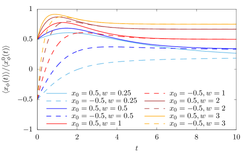
where the propagator $\langle{\phi(x,t)\widetilde{\phi}(x_{0},0)}\rangle$ expressed in terms of the $\mathord{\mathop{\rho}\limits^{\scriptscriptstyle(\sim)}}$ and $\mathord{\mathop{\nu}\limits^{\scriptscriptstyle(\sim)}}$ fields contains the four full propagators, $\langle{\phi\widetilde{\phi}}\rangle=(\leavevmode\hbox to22.34pt{\vbox to3.25pt{\pgfpicture\makeatletter\hbox{\hskip 11.16978pt\lower-1.62271pt\hbox to0.0pt{\pgfsys@beginscope\pgfsys@invoke{ }\definecolor{pgfstrokecolor}{rgb}{0,0,0}\pgfsys@color@rgb@stroke{0}{0}{0}\pgfsys@invoke{ }\pgfsys@color@rgb@fill{0}{0}{0}\pgfsys@invoke{ }\pgfsys@setlinewidth{0.4pt}\pgfsys@invoke{ }\nullfont\pgfsys@beginscope\pgfsys@invoke{ }\pgfsys@invoke{\lxSVG@closescope }\pgfsys@endscope\hbox to0.0pt{\pgfsys@beginscope\pgfsys@invoke{ }{{}}{ {}{{}}{} {}{}\pgfsys@beginscope\pgfsys@invoke{ }\pgfsys@setlinewidth{1.0pt}\pgfsys@invoke{ }\definecolor[named]{pgfstrokecolor}{rgb}{0,0,0}\pgfsys@color@gray@stroke{0}\pgfsys@invoke{ }{}\pgfsys@moveto{10.66978pt}{0.0pt}\pgfsys@lineto{-10.66978pt}{0.0pt}\pgfsys@stroke\pgfsys@invoke{ } \pgfsys@invoke{\lxSVG@closescope }\pgfsys@endscope{}{{}}{}{{{}}{}{}{}{}{}{}{}{}}\pgfsys@beginscope\pgfsys@invoke{ }\color[rgb]{0,0,0}\definecolor[named]{pgfstrokecolor}{rgb}{0,0,0}\pgfsys@color@gray@stroke{0}\pgfsys@invoke{ }\pgfsys@color@gray@fill{0}\pgfsys@invoke{ }\definecolor[named]{pgffillcolor}{rgb}{0,0,0}\definecolor[named]{pgffillcolor}{rgb}{0,0,0}\pgfsys@color@gray@fill{0}\pgfsys@invoke{ }{}\pgfsys@moveto{0.0pt}{0.0pt}\pgfsys@moveto{1.42271pt}{0.0pt}\pgfsys@curveto{1.42271pt}{0.78575pt}{0.78575pt}{1.42271pt}{0.0pt}{1.42271pt}\pgfsys@curveto{-0.78575pt}{1.42271pt}{-1.42271pt}{0.78575pt}{-1.42271pt}{0.0pt}\pgfsys@curveto{-1.42271pt}{-0.78575pt}{-0.78575pt}{-1.42271pt}{0.0pt}{-1.42271pt}\pgfsys@curveto{0.78575pt}{-1.42271pt}{1.42271pt}{-0.78575pt}{1.42271pt}{0.0pt}\pgfsys@closepath\pgfsys@moveto{0.0pt}{0.0pt}\pgfsys@fillstroke\pgfsys@invoke{ } \pgfsys@invoke{\lxSVG@closescope }\pgfsys@endscope} \pgfsys@invoke{\lxSVG@closescope }\pgfsys@endscope{}{}{}\hss}\pgfsys@discardpath\pgfsys@invoke{\lxSVG@closescope }\pgfsys@endscope\hss}}\lxSVG@closescope\endpgfpicture}}+\leavevmode\hbox to22.34pt{\vbox to3.85pt{\pgfpicture\makeatletter\hbox{\hskip 11.16978pt\lower-1.92264pt\hbox to0.0pt{\pgfsys@beginscope\pgfsys@invoke{ }\definecolor{pgfstrokecolor}{rgb}{0,0,0}\pgfsys@color@rgb@stroke{0}{0}{0}\pgfsys@invoke{ }\pgfsys@color@rgb@fill{0}{0}{0}\pgfsys@invoke{ }\pgfsys@setlinewidth{0.4pt}\pgfsys@invoke{ }\nullfont\pgfsys@beginscope\pgfsys@invoke{ }\pgfsys@invoke{\lxSVG@closescope }\pgfsys@endscope\hbox to0.0pt{\pgfsys@beginscope\pgfsys@invoke{ }{{}}{ {}{{}}{} {}{} {}{{}{}}{}{}{}{{}}{{}}{{}{}}{{}{}}{{{{}{}{{}} }}{{}} {}{}{} }{{{{}{}{{}} }}{{}} {{}{}{}{}} {{}{}{}{}} }{{{{}{}{{}} }}{{}} {{}{}{}{}} {{}{}{}{}} }{{{{}{}{{}} }}{{}} {{}{}{}{}} {{}{}{}{}} }{{{{}{}{{}} }}{{}} {{}{}{}{}} {{}{}{}{}} }{{{{}{}{{}} }}{{}} {{}{}{}{}} {{}{}{}{}} }{{{{}{}{{}} }}{{}} {{}{}{}{}} {{}{}{}{}} }{{{{}{}{{}} }}{{}} {{}{}{}{}} {{}{}{}{}} }{{{{}{}{{}} }}{{}} {{}} } \pgfsys@beginscope\pgfsys@invoke{ }\pgfsys@setlinewidth{1.0pt}\pgfsys@invoke{ }\definecolor[named]{pgfstrokecolor}{rgb}{0,0,0}\pgfsys@color@gray@stroke{0}\pgfsys@invoke{ }{}\pgfsys@moveto{10.66978pt}{0.0pt}\pgfsys@curveto{10.04478pt}{0.0pt}{9.73228pt}{-1.42264pt}{9.10728pt}{-1.42264pt}\pgfsys@curveto{8.65479pt}{-1.42264pt}{8.2648pt}{-0.7284pt}{7.85728pt}{0.0pt}\pgfsys@curveto{7.44978pt}{0.72838pt}{7.05978pt}{1.42264pt}{6.60728pt}{1.42264pt}\pgfsys@curveto{6.15479pt}{1.42264pt}{5.7648pt}{0.7284pt}{5.35728pt}{0.0pt}\pgfsys@curveto{4.94978pt}{-0.72838pt}{4.55978pt}{-1.42264pt}{4.10728pt}{-1.42264pt}\pgfsys@curveto{3.65479pt}{-1.42264pt}{3.2648pt}{-0.7284pt}{2.85728pt}{0.0pt}\pgfsys@curveto{2.44978pt}{0.72838pt}{2.05978pt}{1.42264pt}{1.60728pt}{1.42264pt}\pgfsys@curveto{1.15479pt}{1.42264pt}{0.7648pt}{0.7284pt}{0.35728pt}{0.0pt}\pgfsys@curveto{-0.05022pt}{-0.72838pt}{-0.44022pt}{-1.42264pt}{-0.89272pt}{-1.42264pt}\pgfsys@curveto{-1.34521pt}{-1.42264pt}{-1.7352pt}{-0.7284pt}{-2.14272pt}{0.0pt}\pgfsys@curveto{-2.55022pt}{0.72838pt}{-2.94022pt}{1.42264pt}{-3.39272pt}{1.42264pt}\pgfsys@curveto{-3.84521pt}{1.42264pt}{-4.2352pt}{0.7284pt}{-4.64272pt}{0.0pt}\pgfsys@curveto{-5.05022pt}{-0.72838pt}{-5.44022pt}{-1.42264pt}{-5.89272pt}{-1.42264pt}\pgfsys@curveto{-6.34521pt}{-1.42264pt}{-6.7352pt}{-0.7284pt}{-7.14272pt}{0.0pt}\pgfsys@curveto{-7.55022pt}{0.72838pt}{-7.94022pt}{1.42264pt}{-8.39272pt}{1.42264pt}\pgfsys@lineto{-10.66978pt}{0.0pt}\pgfsys@stroke\pgfsys@invoke{ } \pgfsys@invoke{\lxSVG@closescope }\pgfsys@endscope{}{{}}{}{{{}}{}{}{}{}{}{}{}{}}\pgfsys@beginscope\pgfsys@invoke{ }\color[rgb]{0,0,0}\definecolor[named]{pgfstrokecolor}{rgb}{0,0,0}\pgfsys@color@gray@stroke{0}\pgfsys@invoke{ }\pgfsys@color@gray@fill{0}\pgfsys@invoke{ }\definecolor[named]{pgffillcolor}{rgb}{0,0,0}\definecolor[named]{pgffillcolor}{rgb}{0,0,0}\pgfsys@color@gray@fill{0}\pgfsys@invoke{ }{}\pgfsys@moveto{0.0pt}{0.0pt}\pgfsys@moveto{1.42271pt}{0.0pt}\pgfsys@curveto{1.42271pt}{0.78575pt}{0.78575pt}{1.42271pt}{0.0pt}{1.42271pt}\pgfsys@curveto{-0.78575pt}{1.42271pt}{-1.42271pt}{0.78575pt}{-1.42271pt}{0.0pt}\pgfsys@curveto{-1.42271pt}{-0.78575pt}{-0.78575pt}{-1.42271pt}{0.0pt}{-1.42271pt}\pgfsys@curveto{0.78575pt}{-1.42271pt}{1.42271pt}{-0.78575pt}{1.42271pt}{0.0pt}\pgfsys@closepath\pgfsys@moveto{0.0pt}{0.0pt}\pgfsys@fillstroke\pgfsys@invoke{ } \pgfsys@invoke{\lxSVG@closescope }\pgfsys@endscope} \pgfsys@invoke{\lxSVG@closescope }\pgfsys@endscope{}{}{}\hss}\pgfsys@discardpath\pgfsys@invoke{\lxSVG@closescope }\pgfsys@endscope\hss}}\lxSVG@closescope\endpgfpicture}}+\leavevmode\hbox to22.34pt{\vbox to3.55pt{\pgfpicture\makeatletter\hbox{\hskip 11.16978pt\lower-1.92264pt\hbox to0.0pt{\pgfsys@beginscope\pgfsys@invoke{ }\definecolor{pgfstrokecolor}{rgb}{0,0,0}\pgfsys@color@rgb@stroke{0}{0}{0}\pgfsys@invoke{ }\pgfsys@color@rgb@fill{0}{0}{0}\pgfsys@invoke{ }\pgfsys@setlinewidth{0.4pt}\pgfsys@invoke{ }\nullfont\pgfsys@beginscope\pgfsys@invoke{ }\pgfsys@invoke{\lxSVG@closescope }\pgfsys@endscope\hbox to0.0pt{\pgfsys@beginscope\pgfsys@invoke{ }{{}}{ {}{{}}{} {}{}\pgfsys@beginscope\pgfsys@invoke{ }\pgfsys@setlinewidth{1.0pt}\pgfsys@invoke{ }\definecolor[named]{pgfstrokecolor}{rgb}{0,0,0}\pgfsys@color@gray@stroke{0}\pgfsys@invoke{ }{}\pgfsys@moveto{0.0pt}{0.0pt}\pgfsys@lineto{-10.66978pt}{0.0pt}\pgfsys@stroke\pgfsys@invoke{ } \pgfsys@invoke{\lxSVG@closescope }\pgfsys@endscope{}{{}}{} {}{} {}{{}{}}{}{}{}{{}}{{}}{{}{}}{{}{}}{{{{}{}{{}} }}{{}} {}{}{} }{{{{}{}{{}} }}{{}} {}{}{} }{{{{}{}{{}} }}{{}} {{}} } \pgfsys@beginscope\pgfsys@invoke{ }\pgfsys@setlinewidth{1.0pt}\pgfsys@invoke{ }\definecolor[named]{pgfstrokecolor}{rgb}{0,0,0}\pgfsys@color@gray@stroke{0}\pgfsys@invoke{ }{}\pgfsys@moveto{10.66978pt}{0.0pt}\pgfsys@curveto{10.04478pt}{0.0pt}{9.73228pt}{-1.42264pt}{9.10728pt}{-1.42264pt}\pgfsys@curveto{8.48228pt}{-1.42264pt}{8.16978pt}{0.0pt}{7.54478pt}{0.0pt}\pgfsys@lineto{0.0pt}{0.0pt}\pgfsys@stroke\pgfsys@invoke{ } \pgfsys@invoke{\lxSVG@closescope }\pgfsys@endscope{}{{}}{}{{{}}{}{}{}{}{}{}{}{}}\pgfsys@beginscope\pgfsys@invoke{ }\color[rgb]{0,0,0}\definecolor[named]{pgfstrokecolor}{rgb}{0,0,0}\pgfsys@color@gray@stroke{0}\pgfsys@invoke{ }\pgfsys@color@gray@fill{0}\pgfsys@invoke{ }\definecolor[named]{pgffillcolor}{rgb}{0,0,0}\definecolor[named]{pgffillcolor}{rgb}{0,0,0}\pgfsys@color@gray@fill{0}\pgfsys@invoke{ }{}\pgfsys@moveto{0.0pt}{0.0pt}\pgfsys@moveto{1.42271pt}{0.0pt}\pgfsys@curveto{1.42271pt}{0.78575pt}{0.78575pt}{1.42271pt}{0.0pt}{1.42271pt}\pgfsys@curveto{-0.78575pt}{1.42271pt}{-1.42271pt}{0.78575pt}{-1.42271pt}{0.0pt}\pgfsys@curveto{-1.42271pt}{-0.78575pt}{-0.78575pt}{-1.42271pt}{0.0pt}{-1.42271pt}\pgfsys@curveto{0.78575pt}{-1.42271pt}{1.42271pt}{-0.78575pt}{1.42271pt}{0.0pt}\pgfsys@closepath\pgfsys@moveto{0.0pt}{0.0pt}\pgfsys@fillstroke\pgfsys@invoke{ } \pgfsys@invoke{\lxSVG@closescope }\pgfsys@endscope} \pgfsys@invoke{\lxSVG@closescope }\pgfsys@endscope{}{}{}\hss}\pgfsys@discardpath\pgfsys@invoke{\lxSVG@closescope }\pgfsys@endscope\hss}}\lxSVG@closescope\endpgfpicture}}+\leavevmode\hbox to22.34pt{\vbox to3.85pt{\pgfpicture\makeatletter\hbox{\hskip 11.16978pt\lower-1.92264pt\hbox to0.0pt{\pgfsys@beginscope\pgfsys@invoke{ }\definecolor{pgfstrokecolor}{rgb}{0,0,0}\pgfsys@color@rgb@stroke{0}{0}{0}\pgfsys@invoke{ }\pgfsys@color@rgb@fill{0}{0}{0}\pgfsys@invoke{ }\pgfsys@setlinewidth{0.4pt}\pgfsys@invoke{ }\nullfont\pgfsys@beginscope\pgfsys@invoke{ }\pgfsys@invoke{\lxSVG@closescope }\pgfsys@endscope\hbox to0.0pt{\pgfsys@beginscope\pgfsys@invoke{ }{{}}{ {}{{}}{} {}{}\pgfsys@beginscope\pgfsys@invoke{ }\pgfsys@setlinewidth{1.0pt}\pgfsys@invoke{ }\definecolor[named]{pgfstrokecolor}{rgb}{0,0,0}\pgfsys@color@gray@stroke{0}\pgfsys@invoke{ }{}\pgfsys@moveto{10.66978pt}{0.0pt}\pgfsys@lineto{0.0pt}{0.0pt}\pgfsys@stroke\pgfsys@invoke{ } \pgfsys@invoke{\lxSVG@closescope }\pgfsys@endscope{}{{}}{} {}{} {}{{}{}}{}{}{}{{}}{{}}{{}{}}{{}{}}{{{{}{}{{}} }}{{}} {}{}{} }{{{{}{}{{}} }}{{}} {{}{}{}{}} {{}{}{}{}} }{{{{}{}{{}} }}{{}} {{}{}{}{}} {{}{}{}{}} }{{{{}{}{{}} }}{{}} {{}{}{}{}} {{}{}{}{}} }{{{{}{}{{}} }}{{}} {{}} } \pgfsys@beginscope\pgfsys@invoke{ }\pgfsys@setlinewidth{1.0pt}\pgfsys@invoke{ }\definecolor[named]{pgfstrokecolor}{rgb}{0,0,0}\pgfsys@color@gray@stroke{0}\pgfsys@invoke{ }{}\pgfsys@moveto{0.0pt}{0.0pt}\pgfsys@curveto{-0.625pt}{0.0pt}{-0.9375pt}{-1.42264pt}{-1.5625pt}{-1.42264pt}\pgfsys@curveto{-2.015pt}{-1.42264pt}{-2.40498pt}{-0.7284pt}{-2.8125pt}{0.0pt}\pgfsys@curveto{-3.22pt}{0.72838pt}{-3.61pt}{1.42264pt}{-4.0625pt}{1.42264pt}\pgfsys@curveto{-4.515pt}{1.42264pt}{-4.90498pt}{0.7284pt}{-5.3125pt}{0.0pt}\pgfsys@curveto{-5.72pt}{-0.72838pt}{-6.11pt}{-1.42264pt}{-6.5625pt}{-1.42264pt}\pgfsys@curveto{-7.015pt}{-1.42264pt}{-7.40498pt}{-0.7284pt}{-7.8125pt}{0.0pt}\pgfsys@curveto{-8.22pt}{0.72838pt}{-8.61pt}{1.42264pt}{-9.0625pt}{1.42264pt}\pgfsys@lineto{-10.66978pt}{0.0pt}\pgfsys@stroke\pgfsys@invoke{ } \pgfsys@invoke{\lxSVG@closescope }\pgfsys@endscope{}{{}}{}{{{}}{}{}{}{}{}{}{}{}}\pgfsys@beginscope\pgfsys@invoke{ }\color[rgb]{0,0,0}\definecolor[named]{pgfstrokecolor}{rgb}{0,0,0}\pgfsys@color@gray@stroke{0}\pgfsys@invoke{ }\pgfsys@color@gray@fill{0}\pgfsys@invoke{ }\definecolor[named]{pgffillcolor}{rgb}{0,0,0}\definecolor[named]{pgffillcolor}{rgb}{0,0,0}\pgfsys@color@gray@fill{0}\pgfsys@invoke{ }{}\pgfsys@moveto{0.0pt}{0.0pt}\pgfsys@moveto{1.42271pt}{0.0pt}\pgfsys@curveto{1.42271pt}{0.78575pt}{0.78575pt}{1.42271pt}{0.0pt}{1.42271pt}\pgfsys@curveto{-0.78575pt}{1.42271pt}{-1.42271pt}{0.78575pt}{-1.42271pt}{0.0pt}\pgfsys@curveto{-1.42271pt}{-0.78575pt}{-0.78575pt}{-1.42271pt}{0.0pt}{-1.42271pt}\pgfsys@curveto{0.78575pt}{-1.42271pt}{1.42271pt}{-0.78575pt}{1.42271pt}{0.0pt}\pgfsys@closepath\pgfsys@moveto{0.0pt}{0.0pt}\pgfsys@fillstroke\pgfsys@invoke{ } \pgfsys@invoke{\lxSVG@closescope }\pgfsys@endscope} \pgfsys@invoke{\lxSVG@closescope }\pgfsys@endscope{}{}{}\hss}\pgfsys@discardpath\pgfsys@invoke{\lxSVG@closescope }\pgfsys@endscope\hss}}\lxSVG@closescope\endpgfpicture}})/2$, Equation (22w). Definition (22y) contains a mild abuse of notation that we will keep committing throughout, as the angular brackets were introduced in (5) as a path integral but are expectation over a density in (22y). Since there is an integral over space and $x^{n}$ is a polynomial in $x$, the observable can be written as linear combinations of Hermite polynomials, which simplifies the calculations by virtue of the orthogonality relation in (22an). In particular, for the first three moments, $1=H_{0}\left(x/L\right)$, $x/L=H_{1}\left(x/L\right)$ and $(x/L)^{2}=H_{0}\left(x/L\right)+H_{2}\left(x/L\right)$. Using the representation in (11) and the propagators derived in B, the zeroth, first (see figure 2) and second moments are

$$\left\langle{x_{\phi}^{0}(t)}\right\rangle=\frac{\widetilde{u}_{0}(x_{0})}{2L^{2}}\int_{-\infty}^{\infty}\mathchoice{\!\text{d}x\,}{\!\text{d}x\,}{\!\text{d}x\,}{\!\text{d}x\,}H_{0}\left(\frac{x}{L}\right)u_{0}(x)\left(\leavevmode\hbox to50.23pt{\vbox to16.05pt{\pgfpicture\makeatletter\hbox{\hskip 24.76544pt\lower-0.5pt\hbox to0.0pt{\pgfsys@beginscope\pgfsys@invoke{ }\definecolor{pgfstrokecolor}{rgb}{0,0,0}\pgfsys@color@rgb@stroke{0}{0}{0}\pgfsys@invoke{ }\pgfsys@color@rgb@fill{0}{0}{0}\pgfsys@invoke{ }\pgfsys@setlinewidth{0.4pt}\pgfsys@invoke{ }\nullfont\pgfsys@beginscope\pgfsys@invoke{ }\pgfsys@invoke{\lxSVG@closescope }\pgfsys@endscope\hbox to0.0pt{\pgfsys@beginscope\pgfsys@invoke{ }{{}}{ {}{{}}{} {}{}{}{}{{{}{}}}{}{}{{{}{}}}\pgfsys@beginscope\pgfsys@invoke{ }\pgfsys@setlinewidth{1.0pt}\pgfsys@invoke{ }\definecolor[named]{pgfstrokecolor}{rgb}{0,0,0}\pgfsys@color@gray@stroke{0}\pgfsys@invoke{ }{}\pgfsys@moveto{16.00467pt}{0.0pt}\pgfsys@lineto{-16.00467pt}{0.0pt}\pgfsys@stroke\pgfsys@invoke{ }\hbox{\hbox{\hbox{{\pgfsys@beginscope\pgfsys@invoke{ }{{}{}{{ {}{}}}{ {}{}} {{}{{}}}{{}{}}{}{{}{}} { }{{{{}}\pgfsys@beginscope\pgfsys@invoke{ }\pgfsys@transformcm{1.0}{0.0}{0.0}{1.0}{9.88246pt}{5.77745pt}\pgfsys@invoke{ }\hbox{{\definecolor{pgfstrokecolor}{rgb}{0,0,0}\pgfsys@color@rgb@stroke{0}{0}{0}\pgfsys@invoke{ }\pgfsys@color@rgb@fill{0}{0}{0}\pgfsys@invoke{ }\hbox{{${}_{0},0$}} }}\pgfsys@invoke{\lxSVG@closescope }\pgfsys@endscope}}} \pgfsys@invoke{\lxSVG@closescope }\pgfsys@endscope}}}\hbox{{\pgfsys@beginscope\pgfsys@invoke{ }{{}{}{{ {}{}}}{ {}{}} {{}{{}}}{{}{}}{}{{}{}} { }{{{{}}\pgfsys@beginscope\pgfsys@invoke{ }\pgfsys@transformcm{1.0}{0.0}{0.0}{1.0}{-21.43243pt}{5.77744pt}\pgfsys@invoke{ }\hbox{{\definecolor{pgfstrokecolor}{rgb}{0,0,0}\pgfsys@color@rgb@stroke{0}{0}{0}\pgfsys@invoke{ }\pgfsys@color@rgb@fill{0}{0}{0}\pgfsys@invoke{ }\hbox{{${}_{0},t$}} }}\pgfsys@invoke{\lxSVG@closescope }\pgfsys@endscope}}} \pgfsys@invoke{\lxSVG@closescope }\pgfsys@endscope}}} \pgfsys@invoke{\lxSVG@closescope }\pgfsys@endscope} \pgfsys@invoke{\lxSVG@closescope }\pgfsys@endscope{}{}{}\hss}\pgfsys@discardpath\pgfsys@invoke{\lxSVG@closescope }\pgfsys@endscope\hss}}\lxSVG@closescope\endpgfpicture}}+\leavevmode\hbox to50.23pt{\vbox to17.48pt{\pgfpicture\makeatletter\hbox{\hskip 24.76544pt\lower-1.92264pt\hbox to0.0pt{\pgfsys@beginscope\pgfsys@invoke{ }\definecolor{pgfstrokecolor}{rgb}{0,0,0}\pgfsys@color@rgb@stroke{0}{0}{0}\pgfsys@invoke{ }\pgfsys@color@rgb@fill{0}{0}{0}\pgfsys@invoke{ }\pgfsys@setlinewidth{0.4pt}\pgfsys@invoke{ }\nullfont\pgfsys@beginscope\pgfsys@invoke{ }\pgfsys@invoke{\lxSVG@closescope }\pgfsys@endscope\hbox to0.0pt{\pgfsys@beginscope\pgfsys@invoke{ }{{}}{ {}{{}}{} {}{}{}{}{{{}{}}}{}{}{{{}{}}} {}{{}{}}{}{}{}{{}}{{}}{{}{}}{{}{}}{{{{}{}{{}} }}{{}} {}{}{} }{{{{}{}{{}} }}{{}} {{}{}{}{}} {{}{}{}{}} }{{{{}{}{{}} }}{{}} {{}{}{}{}} {{}{}{}{}} }{{{{}{}{{}} }}{{}} {{}{}{}{}} {{}{}{}{}} }{{{{}{}{{}} }}{{}} {{}{}{}{}} {{}{}{}{}} }{{{{}{}{{}} }}{{}} {{}{}{}{}} {{}{}{}{}} }{{{{}{}{{}} }}{{}} {{}{}{}{}} {{}{}{}{}} }{{{{}{}{{}} }}{{}} {{}{}{}{}} {{}{}{}{}} }{{{{}{}{{}} }}{{}} {{}{}{}{}} {{}{}{}{}} }{{{{}{}{{}} }}{{}} {{}{}{}{}} {{}{}{}{}} }{{{{}{}{{}} }}{{}} {{}{}{}{}} {{}{}{}{}} }{{{{}{}{{}} }}{{}} {{}{}{}{}} {{}{}{}{}} }{{{{}{}{{}} }}{{}} {{}} } \pgfsys@beginscope\pgfsys@invoke{ }\pgfsys@setlinewidth{1.0pt}\pgfsys@invoke{ }\definecolor[named]{pgfstrokecolor}{rgb}{0,0,0}\pgfsys@color@gray@stroke{0}\pgfsys@invoke{ }{}\pgfsys@moveto{16.00467pt}{0.0pt}\pgfsys@curveto{15.37967pt}{0.0pt}{15.06717pt}{-1.42264pt}{14.44217pt}{-1.42264pt}\pgfsys@curveto{13.98967pt}{-1.42264pt}{13.59969pt}{-0.7284pt}{13.19217pt}{0.0pt}\pgfsys@curveto{12.78467pt}{0.72838pt}{12.39467pt}{1.42264pt}{11.94217pt}{1.42264pt}\pgfsys@curveto{11.48967pt}{1.42264pt}{11.09969pt}{0.7284pt}{10.69217pt}{0.0pt}\pgfsys@curveto{10.28467pt}{-0.72838pt}{9.89467pt}{-1.42264pt}{9.44217pt}{-1.42264pt}\pgfsys@curveto{8.98967pt}{-1.42264pt}{8.59969pt}{-0.7284pt}{8.19217pt}{0.0pt}\pgfsys@curveto{7.78467pt}{0.72838pt}{7.39467pt}{1.42264pt}{6.94217pt}{1.42264pt}\pgfsys@curveto{6.48967pt}{1.42264pt}{6.09969pt}{0.7284pt}{5.69217pt}{0.0pt}\pgfsys@curveto{5.28467pt}{-0.72838pt}{4.89467pt}{-1.42264pt}{4.44217pt}{-1.42264pt}\pgfsys@curveto{3.98967pt}{-1.42264pt}{3.59969pt}{-0.7284pt}{3.19217pt}{0.0pt}\pgfsys@curveto{2.78467pt}{0.72838pt}{2.39467pt}{1.42264pt}{1.94217pt}{1.42264pt}\pgfsys@curveto{1.48967pt}{1.42264pt}{1.09969pt}{0.7284pt}{0.69217pt}{0.0pt}\pgfsys@curveto{0.28467pt}{-0.72838pt}{-0.10533pt}{-1.42264pt}{-0.55783pt}{-1.42264pt}\pgfsys@curveto{-1.01033pt}{-1.42264pt}{-1.40031pt}{-0.7284pt}{-1.80783pt}{0.0pt}\pgfsys@curveto{-2.21533pt}{0.72838pt}{-2.60533pt}{1.42264pt}{-3.05783pt}{1.42264pt}\pgfsys@curveto{-3.51033pt}{1.42264pt}{-3.90031pt}{0.7284pt}{-4.30783pt}{0.0pt}\pgfsys@curveto{-4.71533pt}{-0.72838pt}{-5.10533pt}{-1.42264pt}{-5.55783pt}{-1.42264pt}\pgfsys@curveto{-6.01033pt}{-1.42264pt}{-6.40031pt}{-0.7284pt}{-6.80783pt}{0.0pt}\pgfsys@curveto{-7.21533pt}{0.72838pt}{-7.60533pt}{1.42264pt}{-8.05783pt}{1.42264pt}\pgfsys@curveto{-8.51033pt}{1.42264pt}{-8.90031pt}{0.7284pt}{-9.30783pt}{0.0pt}\pgfsys@curveto{-9.71533pt}{-0.72838pt}{-10.10533pt}{-1.42264pt}{-10.55783pt}{-1.42264pt}\pgfsys@curveto{-11.01033pt}{-1.42264pt}{-11.40031pt}{-0.7284pt}{-11.80783pt}{0.0pt}\pgfsys@curveto{-12.21533pt}{0.72838pt}{-12.60533pt}{1.42264pt}{-13.05783pt}{1.42264pt}\pgfsys@lineto{-16.00467pt}{0.0pt}\pgfsys@stroke\pgfsys@invoke{ }\hbox{\hbox{\hbox{{\pgfsys@beginscope\pgfsys@invoke{ }{{}{}{{ {}{}}}{ {}{}} {{}{{}}}{{}{}}{}{{}{}} { }{{{{}}\pgfsys@beginscope\pgfsys@invoke{ }\pgfsys@transformcm{1.0}{0.0}{0.0}{1.0}{9.88246pt}{5.77745pt}\pgfsys@invoke{ }\hbox{{\definecolor{pgfstrokecolor}{rgb}{0,0,0}\pgfsys@color@rgb@stroke{0}{0}{0}\pgfsys@invoke{ }\pgfsys@color@rgb@fill{0}{0}{0}\pgfsys@invoke{ }\hbox{{${}_{0},0$}} }}\pgfsys@invoke{\lxSVG@closescope }\pgfsys@endscope}}} \pgfsys@invoke{\lxSVG@closescope }\pgfsys@endscope}}}\hbox{{\pgfsys@beginscope\pgfsys@invoke{ }{{}{}{{ {}{}}}{ {}{}} {{}{{}}}{{}{}}{}{{}{}} { }{{{{}}\pgfsys@beginscope\pgfsys@invoke{ }\pgfsys@transformcm{1.0}{0.0}{0.0}{1.0}{-21.43243pt}{5.77744pt}\pgfsys@invoke{ }\hbox{{\definecolor{pgfstrokecolor}{rgb}{0,0,0}\pgfsys@color@rgb@stroke{0}{0}{0}\pgfsys@invoke{ }\pgfsys@color@rgb@fill{0}{0}{0}\pgfsys@invoke{ }\hbox{{${}_{0},t$}} }}\pgfsys@invoke{\lxSVG@closescope }\pgfsys@endscope}}} \pgfsys@invoke{\lxSVG@closescope }\pgfsys@endscope}}} \pgfsys@invoke{\lxSVG@closescope }\pgfsys@endscope} \pgfsys@invoke{\lxSVG@closescope }\pgfsys@endscope{}{}{}\hss}\pgfsys@discardpath\pgfsys@invoke{\lxSVG@closescope }\pgfsys@endscope\hss}}\lxSVG@closescope\endpgfpicture}}\right) {}_{0},0 {}_{0},t {}_{0},0 {}_{0},t {}_{0},0 {}_{0},t {}_{0},0 {}_{0},t$$

$$=\frac{1}{2}\left(1+\mathchoice{e^{-\alpha t}}{\operatorname{exp}\!\left(-\alpha t\right)}{\operatorname{exp}\!\left(-\alpha t\right)}{\operatorname{exp}\!\left(-\alpha t\right)}\right)\,,$$ (22za)

$$\left\langle{x_{\phi}(t)}\right\rangle=\frac{1}{2L}\int_{-\infty}^{\infty}\mathchoice{\!\text{d}x\,}{\!\text{d}x\,}{\!\text{d}x\,}{\!\text{d}x\,}H_{1}\left(\frac{x}{L}\right)u_{1}(x)$$

$$\times\left[\left(\leavevmode\hbox to50.23pt{\vbox to16.05pt{\pgfpicture\makeatletter\hbox{\hskip 24.76544pt\lower-0.5pt\hbox to0.0pt{\pgfsys@beginscope\pgfsys@invoke{ }\definecolor{pgfstrokecolor}{rgb}{0,0,0}\pgfsys@color@rgb@stroke{0}{0}{0}\pgfsys@invoke{ }\pgfsys@color@rgb@fill{0}{0}{0}\pgfsys@invoke{ }\pgfsys@setlinewidth{0.4pt}\pgfsys@invoke{ }\nullfont\pgfsys@beginscope\pgfsys@invoke{ }\pgfsys@invoke{\lxSVG@closescope }\pgfsys@endscope\hbox to0.0pt{\pgfsys@beginscope\pgfsys@invoke{ }{{}}{ {}{{}}{} {}{}{}{}{{{}{}}}{}{}{{{}{}}}\pgfsys@beginscope\pgfsys@invoke{ }\pgfsys@setlinewidth{1.0pt}\pgfsys@invoke{ }\definecolor[named]{pgfstrokecolor}{rgb}{0,0,0}\pgfsys@color@gray@stroke{0}\pgfsys@invoke{ }{}\pgfsys@moveto{16.00467pt}{0.0pt}\pgfsys@lineto{-16.00467pt}{0.0pt}\pgfsys@stroke\pgfsys@invoke{ }\hbox{\hbox{\hbox{{\pgfsys@beginscope\pgfsys@invoke{ }{{}{}{{ {}{}}}{ {}{}} {{}{{}}}{{}{}}{}{{}{}} { }{{{{}}\pgfsys@beginscope\pgfsys@invoke{ }\pgfsys@transformcm{1.0}{0.0}{0.0}{1.0}{9.88246pt}{5.77745pt}\pgfsys@invoke{ }\hbox{{\definecolor{pgfstrokecolor}{rgb}{0,0,0}\pgfsys@color@rgb@stroke{0}{0}{0}\pgfsys@invoke{ }\pgfsys@color@rgb@fill{0}{0}{0}\pgfsys@invoke{ }\hbox{{${}_{1},0$}} }}\pgfsys@invoke{\lxSVG@closescope }\pgfsys@endscope}}} \pgfsys@invoke{\lxSVG@closescope }\pgfsys@endscope}}}\hbox{{\pgfsys@beginscope\pgfsys@invoke{ }{{}{}{{ {}{}}}{ {}{}} {{}{{}}}{{}{}}{}{{}{}} { }{{{{}}\pgfsys@beginscope\pgfsys@invoke{ }\pgfsys@transformcm{1.0}{0.0}{0.0}{1.0}{-21.43243pt}{5.77744pt}\pgfsys@invoke{ }\hbox{{\definecolor{pgfstrokecolor}{rgb}{0,0,0}\pgfsys@color@rgb@stroke{0}{0}{0}\pgfsys@invoke{ }\pgfsys@color@rgb@fill{0}{0}{0}\pgfsys@invoke{ }\hbox{{${}_{1},t$}} }}\pgfsys@invoke{\lxSVG@closescope }\pgfsys@endscope}}} \pgfsys@invoke{\lxSVG@closescope }\pgfsys@endscope}}} \pgfsys@invoke{\lxSVG@closescope }\pgfsys@endscope} \pgfsys@invoke{\lxSVG@closescope }\pgfsys@endscope{}{}{}\hss}\pgfsys@discardpath\pgfsys@invoke{\lxSVG@closescope }\pgfsys@endscope\hss}}\lxSVG@closescope\endpgfpicture}}+\leavevmode\hbox to50.23pt{\vbox to17.48pt{\pgfpicture\makeatletter\hbox{\hskip 24.76544pt\lower-1.92264pt\hbox to0.0pt{\pgfsys@beginscope\pgfsys@invoke{ }\definecolor{pgfstrokecolor}{rgb}{0,0,0}\pgfsys@color@rgb@stroke{0}{0}{0}\pgfsys@invoke{ }\pgfsys@color@rgb@fill{0}{0}{0}\pgfsys@invoke{ }\pgfsys@setlinewidth{0.4pt}\pgfsys@invoke{ }\nullfont\pgfsys@beginscope\pgfsys@invoke{ }\pgfsys@invoke{\lxSVG@closescope }\pgfsys@endscope\hbox to0.0pt{\pgfsys@beginscope\pgfsys@invoke{ }{{}}{ {}{{}}{} {}{}{}{}{{{}{}}}{}{}{{{}{}}} {}{{}{}}{}{}{}{{}}{{}}{{}{}}{{}{}}{{{{}{}{{}} }}{{}} {}{}{} }{{{{}{}{{}} }}{{}} {{}{}{}{}} {{}{}{}{}} }{{{{}{}{{}} }}{{}} {{}{}{}{}} {{}{}{}{}} }{{{{}{}{{}} }}{{}} {{}{}{}{}} {{}{}{}{}} }{{{{}{}{{}} }}{{}} {{}{}{}{}} {{}{}{}{}} }{{{{}{}{{}} }}{{}} {{}{}{}{}} {{}{}{}{}} }{{{{}{}{{}} }}{{}} {{}{}{}{}} {{}{}{}{}} }{{{{}{}{{}} }}{{}} {{}{}{}{}} {{}{}{}{}} }{{{{}{}{{}} }}{{}} {{}{}{}{}} {{}{}{}{}} }{{{{}{}{{}} }}{{}} {{}{}{}{}} {{}{}{}{}} }{{{{}{}{{}} }}{{}} {{}{}{}{}} {{}{}{}{}} }{{{{}{}{{}} }}{{}} {{}{}{}{}} {{}{}{}{}} }{{{{}{}{{}} }}{{}} {{}} } \pgfsys@beginscope\pgfsys@invoke{ }\pgfsys@setlinewidth{1.0pt}\pgfsys@invoke{ }\definecolor[named]{pgfstrokecolor}{rgb}{0,0,0}\pgfsys@color@gray@stroke{0}\pgfsys@invoke{ }{}\pgfsys@moveto{16.00467pt}{0.0pt}\pgfsys@curveto{15.37967pt}{0.0pt}{15.06717pt}{-1.42264pt}{14.44217pt}{-1.42264pt}\pgfsys@curveto{13.98967pt}{-1.42264pt}{13.59969pt}{-0.7284pt}{13.19217pt}{0.0pt}\pgfsys@curveto{12.78467pt}{0.72838pt}{12.39467pt}{1.42264pt}{11.94217pt}{1.42264pt}\pgfsys@curveto{11.48967pt}{1.42264pt}{11.09969pt}{0.7284pt}{10.69217pt}{0.0pt}\pgfsys@curveto{10.28467pt}{-0.72838pt}{9.89467pt}{-1.42264pt}{9.44217pt}{-1.42264pt}\pgfsys@curveto{8.98967pt}{-1.42264pt}{8.59969pt}{-0.7284pt}{8.19217pt}{0.0pt}\pgfsys@curveto{7.78467pt}{0.72838pt}{7.39467pt}{1.42264pt}{6.94217pt}{1.42264pt}\pgfsys@curveto{6.48967pt}{1.42264pt}{6.09969pt}{0.7284pt}{5.69217pt}{0.0pt}\pgfsys@curveto{5.28467pt}{-0.72838pt}{4.89467pt}{-1.42264pt}{4.44217pt}{-1.42264pt}\pgfsys@curveto{3.98967pt}{-1.42264pt}{3.59969pt}{-0.7284pt}{3.19217pt}{0.0pt}\pgfsys@curveto{2.78467pt}{0.72838pt}{2.39467pt}{1.42264pt}{1.94217pt}{1.42264pt}\pgfsys@curveto{1.48967pt}{1.42264pt}{1.09969pt}{0.7284pt}{0.69217pt}{0.0pt}\pgfsys@curveto{0.28467pt}{-0.72838pt}{-0.10533pt}{-1.42264pt}{-0.55783pt}{-1.42264pt}\pgfsys@curveto{-1.01033pt}{-1.42264pt}{-1.40031pt}{-0.7284pt}{-1.80783pt}{0.0pt}\pgfsys@curveto{-2.21533pt}{0.72838pt}{-2.60533pt}{1.42264pt}{-3.05783pt}{1.42264pt}\pgfsys@curveto{-3.51033pt}{1.42264pt}{-3.90031pt}{0.7284pt}{-4.30783pt}{0.0pt}\pgfsys@curveto{-4.71533pt}{-0.72838pt}{-5.10533pt}{-1.42264pt}{-5.55783pt}{-1.42264pt}\pgfsys@curveto{-6.01033pt}{-1.42264pt}{-6.40031pt}{-0.7284pt}{-6.80783pt}{0.0pt}\pgfsys@curveto{-7.21533pt}{0.72838pt}{-7.60533pt}{1.42264pt}{-8.05783pt}{1.42264pt}\pgfsys@curveto{-8.51033pt}{1.42264pt}{-8.90031pt}{0.7284pt}{-9.30783pt}{0.0pt}\pgfsys@curveto{-9.71533pt}{-0.72838pt}{-10.10533pt}{-1.42264pt}{-10.55783pt}{-1.42264pt}\pgfsys@curveto{-11.01033pt}{-1.42264pt}{-11.40031pt}{-0.7284pt}{-11.80783pt}{0.0pt}\pgfsys@curveto{-12.21533pt}{0.72838pt}{-12.60533pt}{1.42264pt}{-13.05783pt}{1.42264pt}\pgfsys@lineto{-16.00467pt}{0.0pt}\pgfsys@stroke\pgfsys@invoke{ }\hbox{\hbox{\hbox{{\pgfsys@beginscope\pgfsys@invoke{ }{{}{}{{ {}{}}}{ {}{}} {{}{{}}}{{}{}}{}{{}{}} { }{{{{}}\pgfsys@beginscope\pgfsys@invoke{ }\pgfsys@transformcm{1.0}{0.0}{0.0}{1.0}{9.88246pt}{5.77745pt}\pgfsys@invoke{ }\hbox{{\definecolor{pgfstrokecolor}{rgb}{0,0,0}\pgfsys@color@rgb@stroke{0}{0}{0}\pgfsys@invoke{ }\pgfsys@color@rgb@fill{0}{0}{0}\pgfsys@invoke{ }\hbox{{${}_{1},0$}} }}\pgfsys@invoke{\lxSVG@closescope }\pgfsys@endscope}}} \pgfsys@invoke{\lxSVG@closescope }\pgfsys@endscope}}}\hbox{{\pgfsys@beginscope\pgfsys@invoke{ }{{}{}{{ {}{}}}{ {}{}} {{}{{}}}{{}{}}{}{{}{}} { }{{{{}}\pgfsys@beginscope\pgfsys@invoke{ }\pgfsys@transformcm{1.0}{0.0}{0.0}{1.0}{-21.43243pt}{5.77744pt}\pgfsys@invoke{ }\hbox{{\definecolor{pgfstrokecolor}{rgb}{0,0,0}\pgfsys@color@rgb@stroke{0}{0}{0}\pgfsys@invoke{ }\pgfsys@color@rgb@fill{0}{0}{0}\pgfsys@invoke{ }\hbox{{${}_{1},t$}} }}\pgfsys@invoke{\lxSVG@closescope }\pgfsys@endscope}}} \pgfsys@invoke{\lxSVG@closescope }\pgfsys@endscope}}} \pgfsys@invoke{\lxSVG@closescope }\pgfsys@endscope} \pgfsys@invoke{\lxSVG@closescope }\pgfsys@endscope{}{}{}\hss}\pgfsys@discardpath\pgfsys@invoke{\lxSVG@closescope }\pgfsys@endscope\hss}}\lxSVG@closescope\endpgfpicture}}\right)\widetilde{u}_{1}(x_{0})+\left(\leavevmode\hbox to50.23pt{\vbox to17.48pt{\pgfpicture\makeatletter\hbox{\hskip 24.76544pt\lower-1.92264pt\hbox to0.0pt{\pgfsys@beginscope\pgfsys@invoke{ }\definecolor{pgfstrokecolor}{rgb}{0,0,0}\pgfsys@color@rgb@stroke{0}{0}{0}\pgfsys@invoke{ }\pgfsys@color@rgb@fill{0}{0}{0}\pgfsys@invoke{ }\pgfsys@setlinewidth{0.4pt}\pgfsys@invoke{ }\nullfont\pgfsys@beginscope\pgfsys@invoke{ }\pgfsys@invoke{\lxSVG@closescope }\pgfsys@endscope\hbox to0.0pt{\pgfsys@beginscope\pgfsys@invoke{ }{{}}{ {}{{}}{} {}{}{}{}{{{}{}}}\pgfsys@beginscope\pgfsys@invoke{ }\pgfsys@setlinewidth{1.0pt}\pgfsys@invoke{ }\definecolor[named]{pgfstrokecolor}{rgb}{0,0,0}\pgfsys@color@gray@stroke{0}\pgfsys@invoke{ }{}\pgfsys@moveto{0.0pt}{0.0pt}\pgfsys@lineto{-16.00467pt}{0.0pt}\pgfsys@stroke\pgfsys@invoke{ }\hbox{\hbox{{\pgfsys@beginscope\pgfsys@invoke{ }{{}{}{{ {}{}}}{ {}{}} {{}{{}}}{{}{}}{}{{}{}} { }{{{{}}\pgfsys@beginscope\pgfsys@invoke{ }\pgfsys@transformcm{1.0}{0.0}{0.0}{1.0}{-21.43243pt}{5.77744pt}\pgfsys@invoke{ }\hbox{{\definecolor{pgfstrokecolor}{rgb}{0,0,0}\pgfsys@color@rgb@stroke{0}{0}{0}\pgfsys@invoke{ }\pgfsys@color@rgb@fill{0}{0}{0}\pgfsys@invoke{ }\hbox{{${}_{1},t$}} }}\pgfsys@invoke{\lxSVG@closescope }\pgfsys@endscope}}} \pgfsys@invoke{\lxSVG@closescope }\pgfsys@endscope}}} \pgfsys@invoke{\lxSVG@closescope }\pgfsys@endscope{}{{}}{} {}{}{}{}{{{}{}}} {}{{}{}}{}{}{}{{}}{{}}{{}{}}{{}{}}{{{{}{}{{}} }}{{}} {}{}{} }{{{{}{}{{}} }}{{}} {}{}{} }{{{{}{}{{}} }}{{}} {{}} } \pgfsys@beginscope\pgfsys@invoke{ }\pgfsys@setlinewidth{1.0pt}\pgfsys@invoke{ }\definecolor[named]{pgfstrokecolor}{rgb}{0,0,0}\pgfsys@color@gray@stroke{0}\pgfsys@invoke{ }{}\pgfsys@moveto{16.00467pt}{0.0pt}\pgfsys@curveto{15.37967pt}{0.0pt}{15.06717pt}{-1.42264pt}{14.44217pt}{-1.42264pt}\pgfsys@curveto{13.81717pt}{-1.42264pt}{13.50467pt}{0.0pt}{12.87967pt}{0.0pt}\pgfsys@lineto{0.0pt}{0.0pt}\pgfsys@stroke\pgfsys@invoke{ }\hbox{\hbox{{\pgfsys@beginscope\pgfsys@invoke{ }{{}{}{{ {}{}}}{ {}{}} {{}{{}}}{{}{}}{}{{}{}} { }{{{{}}\pgfsys@beginscope\pgfsys@invoke{ }\pgfsys@transformcm{1.0}{0.0}{0.0}{1.0}{9.88246pt}{5.77745pt}\pgfsys@invoke{ }\hbox{{\definecolor{pgfstrokecolor}{rgb}{0,0,0}\pgfsys@color@rgb@stroke{0}{0}{0}\pgfsys@invoke{ }\pgfsys@color@rgb@fill{0}{0}{0}\pgfsys@invoke{ }\hbox{{${}_{0},0$}} }}\pgfsys@invoke{\lxSVG@closescope }\pgfsys@endscope}}} \pgfsys@invoke{\lxSVG@closescope }\pgfsys@endscope}}} \pgfsys@invoke{\lxSVG@closescope }\pgfsys@endscope} \pgfsys@invoke{\lxSVG@closescope }\pgfsys@endscope{}{}{}\hss}\pgfsys@discardpath\pgfsys@invoke{\lxSVG@closescope }\pgfsys@endscope\hss}}\lxSVG@closescope\endpgfpicture}}+\leavevmode\hbox to50.23pt{\vbox to17.48pt{\pgfpicture\makeatletter\hbox{\hskip 24.76544pt\lower-1.92264pt\hbox to0.0pt{\pgfsys@beginscope\pgfsys@invoke{ }\definecolor{pgfstrokecolor}{rgb}{0,0,0}\pgfsys@color@rgb@stroke{0}{0}{0}\pgfsys@invoke{ }\pgfsys@color@rgb@fill{0}{0}{0}\pgfsys@invoke{ }\pgfsys@setlinewidth{0.4pt}\pgfsys@invoke{ }\nullfont\pgfsys@beginscope\pgfsys@invoke{ }\pgfsys@invoke{\lxSVG@closescope }\pgfsys@endscope\hbox to0.0pt{\pgfsys@beginscope\pgfsys@invoke{ }{{}}{ {}{{}}{} {}{}{}{}{{{}{}}} {}{{}{}}{}{}{}{{}}{{}}{{}{}}{{}{}}{{{{}{}{{}} }}{{}} {}{}{} }{{{{}{}{{}} }}{{}} {{}{}{}{}} {{}{}{}{}} }{{{{}{}{{}} }}{{}} {{}{}{}{}} {{}{}{}{}} }{{{{}{}{{}} }}{{}} {{}{}{}{}} {{}{}{}{}} }{{{{}{}{{}} }}{{}} {{}{}{}{}} {{}{}{}{}} }{{{{}{}{{}} }}{{}} {{}{}{}{}} {{}{}{}{}} }{{{{}{}{{}} }}{{}} {{}} } \pgfsys@beginscope\pgfsys@invoke{ }\pgfsys@setlinewidth{1.0pt}\pgfsys@invoke{ }\definecolor[named]{pgfstrokecolor}{rgb}{0,0,0}\pgfsys@color@gray@stroke{0}\pgfsys@invoke{ }{}\pgfsys@moveto{0.0pt}{0.0pt}\pgfsys@curveto{-0.625pt}{0.0pt}{-0.9375pt}{-1.42264pt}{-1.5625pt}{-1.42264pt}\pgfsys@curveto{-2.015pt}{-1.42264pt}{-2.40498pt}{-0.7284pt}{-2.8125pt}{0.0pt}\pgfsys@curveto{-3.22pt}{0.72838pt}{-3.61pt}{1.42264pt}{-4.0625pt}{1.42264pt}\pgfsys@curveto{-4.515pt}{1.42264pt}{-4.90498pt}{0.7284pt}{-5.3125pt}{0.0pt}\pgfsys@curveto{-5.72pt}{-0.72838pt}{-6.11pt}{-1.42264pt}{-6.5625pt}{-1.42264pt}\pgfsys@curveto{-7.015pt}{-1.42264pt}{-7.40498pt}{-0.7284pt}{-7.8125pt}{0.0pt}\pgfsys@curveto{-8.22pt}{0.72838pt}{-8.61pt}{1.42264pt}{-9.0625pt}{1.42264pt}\pgfsys@curveto{-9.515pt}{1.42264pt}{-9.90498pt}{0.7284pt}{-10.3125pt}{0.0pt}\pgfsys@curveto{-10.72pt}{-0.72838pt}{-11.11pt}{-1.42264pt}{-11.5625pt}{-1.42264pt}\pgfsys@curveto{-12.015pt}{-1.42264pt}{-12.40498pt}{-0.7284pt}{-12.8125pt}{0.0pt}\pgfsys@curveto{-13.22pt}{0.72838pt}{-13.61pt}{1.42264pt}{-14.0625pt}{1.42264pt}\pgfsys@lineto{-16.00467pt}{0.0pt}\pgfsys@stroke\pgfsys@invoke{ }\hbox{\hbox{{\pgfsys@beginscope\pgfsys@invoke{ }{{}{}{{ {}{}}}{ {}{}} {{}{{}}}{{}{}}{}{{}{}} { }{{{{}}\pgfsys@beginscope\pgfsys@invoke{ }\pgfsys@transformcm{1.0}{0.0}{0.0}{1.0}{-21.43243pt}{5.77744pt}\pgfsys@invoke{ }\hbox{{\definecolor{pgfstrokecolor}{rgb}{0,0,0}\pgfsys@color@rgb@stroke{0}{0}{0}\pgfsys@invoke{ }\pgfsys@color@rgb@fill{0}{0}{0}\pgfsys@invoke{ }\hbox{{${}_{1},t$}} }}\pgfsys@invoke{\lxSVG@closescope }\pgfsys@endscope}}} \pgfsys@invoke{\lxSVG@closescope }\pgfsys@endscope}}} \pgfsys@invoke{\lxSVG@closescope }\pgfsys@endscope{}{{}}{} {}{}{}{}{{{}{}}}\pgfsys@beginscope\pgfsys@invoke{ }\pgfsys@setlinewidth{1.0pt}\pgfsys@invoke{ }\definecolor[named]{pgfstrokecolor}{rgb}{0,0,0}\pgfsys@color@gray@stroke{0}\pgfsys@invoke{ }{}\pgfsys@moveto{16.00467pt}{0.0pt}\pgfsys@lineto{0.0pt}{0.0pt}\pgfsys@stroke\pgfsys@invoke{ }\hbox{\hbox{{\pgfsys@beginscope\pgfsys@invoke{ }{{}{}{{ {}{}}}{ {}{}} {{}{{}}}{{}{}}{}{{}{}} { }{{{{}}\pgfsys@beginscope\pgfsys@invoke{ }\pgfsys@transformcm{1.0}{0.0}{0.0}{1.0}{9.88246pt}{5.77745pt}\pgfsys@invoke{ }\hbox{{\definecolor{pgfstrokecolor}{rgb}{0,0,0}\pgfsys@color@rgb@stroke{0}{0}{0}\pgfsys@invoke{ }\pgfsys@color@rgb@fill{0}{0}{0}\pgfsys@invoke{ }\hbox{{${}_{0},0$}} }}\pgfsys@invoke{\lxSVG@closescope }\pgfsys@endscope}}} \pgfsys@invoke{\lxSVG@closescope }\pgfsys@endscope}}} \pgfsys@invoke{\lxSVG@closescope }\pgfsys@endscope} \pgfsys@invoke{\lxSVG@closescope }\pgfsys@endscope{}{}{}\hss}\pgfsys@discardpath\pgfsys@invoke{\lxSVG@closescope }\pgfsys@endscope\hss}}\lxSVG@closescope\endpgfpicture}}\right)\widetilde{u}_{0}(x_{0})\right] {}_{1},0 {}_{1},t {}_{1},0 {}_{1},t {}_{1},t {}_{0},0 {}_{1},t {}_{0},0 {}_{1},0 {}_{1},t {}_{1},0 {}_{1},t {}_{1},t {}_{0},0 {}_{1},t {}_{0},0$$

$$=\frac{x_{0}}{2}\mathchoice{e^{-kt}}{\operatorname{exp}\!\left(-kt\right)}{\operatorname{exp}\!\left(-kt\right)}{\operatorname{exp}\!\left(-kt\right)}\left(1+\mathchoice{e^{-\alpha t}}{\operatorname{exp}\!\left(-\alpha t\right)}{\operatorname{exp}\!\left(-\alpha t\right)}{\operatorname{exp}\!\left(-\alpha t\right)}\right)+\frac{w}{2}\left(\frac{1}{k-\alpha}\left(\mathchoice{e^{-\alpha t}}{\operatorname{exp}\!\left(-\alpha t\right)}{\operatorname{exp}\!\left(-\alpha t\right)}{\operatorname{exp}\!\left(-\alpha t\right)}-\mathchoice{e^{-kt}}{\operatorname{exp}\!\left(-kt\right)}{\operatorname{exp}\!\left(-kt\right)}{\operatorname{exp}\!\left(-kt\right)}\right)+\frac{1}{k+\alpha}\left(1-\mathchoice{e^{-(k+\alpha)t}}{\operatorname{exp}\!\left(-(k+\alpha)t\right)}{\operatorname{exp}\!\left(-(k+\alpha)t\right)}{\operatorname{exp}\!\left(-(k+\alpha)t\right)}\right)\right)\,,$$ (22zb)

$$\left\langle{x_{\phi}^{2}(t)}\right\rangle=\frac{1}{2}\left[\int_{-\infty}^{\infty}\mathchoice{\!\text{d}x\,}{\!\text{d}x\,}{\!\text{d}x\,}{\!\text{d}x\,}H_{0}\left(\frac{x}{L}\right)u_{0}(x)\right.\left(\leavevmode\hbox to50.23pt{\vbox to16.05pt{\pgfpicture\makeatletter\hbox{\hskip 24.76544pt\lower-0.5pt\hbox to0.0pt{\pgfsys@beginscope\pgfsys@invoke{ }\definecolor{pgfstrokecolor}{rgb}{0,0,0}\pgfsys@color@rgb@stroke{0}{0}{0}\pgfsys@invoke{ }\pgfsys@color@rgb@fill{0}{0}{0}\pgfsys@invoke{ }\pgfsys@setlinewidth{0.4pt}\pgfsys@invoke{ }\nullfont\pgfsys@beginscope\pgfsys@invoke{ }\pgfsys@invoke{\lxSVG@closescope }\pgfsys@endscope\hbox to0.0pt{\pgfsys@beginscope\pgfsys@invoke{ }{{}}{ {}{{}}{} {}{}{}{}{{{}{}}}{}{}{{{}{}}}\pgfsys@beginscope\pgfsys@invoke{ }\pgfsys@setlinewidth{1.0pt}\pgfsys@invoke{ }\definecolor[named]{pgfstrokecolor}{rgb}{0,0,0}\pgfsys@color@gray@stroke{0}\pgfsys@invoke{ }{}\pgfsys@moveto{16.00467pt}{0.0pt}\pgfsys@lineto{-16.00467pt}{0.0pt}\pgfsys@stroke\pgfsys@invoke{ }\hbox{\hbox{\hbox{{\pgfsys@beginscope\pgfsys@invoke{ }{{}{}{{ {}{}}}{ {}{}} {{}{{}}}{{}{}}{}{{}{}} { }{{{{}}\pgfsys@beginscope\pgfsys@invoke{ }\pgfsys@transformcm{1.0}{0.0}{0.0}{1.0}{9.88246pt}{5.77745pt}\pgfsys@invoke{ }\hbox{{\definecolor{pgfstrokecolor}{rgb}{0,0,0}\pgfsys@color@rgb@stroke{0}{0}{0}\pgfsys@invoke{ }\pgfsys@color@rgb@fill{0}{0}{0}\pgfsys@invoke{ }\hbox{{${}_{0},0$}} }}\pgfsys@invoke{\lxSVG@closescope }\pgfsys@endscope}}} \pgfsys@invoke{\lxSVG@closescope }\pgfsys@endscope}}}\hbox{{\pgfsys@beginscope\pgfsys@invoke{ }{{}{}{{ {}{}}}{ {}{}} {{}{{}}}{{}{}}{}{{}{}} { }{{{{}}\pgfsys@beginscope\pgfsys@invoke{ }\pgfsys@transformcm{1.0}{0.0}{0.0}{1.0}{-21.43243pt}{5.77744pt}\pgfsys@invoke{ }\hbox{{\definecolor{pgfstrokecolor}{rgb}{0,0,0}\pgfsys@color@rgb@stroke{0}{0}{0}\pgfsys@invoke{ }\pgfsys@color@rgb@fill{0}{0}{0}\pgfsys@invoke{ }\hbox{{${}_{0},t$}} }}\pgfsys@invoke{\lxSVG@closescope }\pgfsys@endscope}}} \pgfsys@invoke{\lxSVG@closescope }\pgfsys@endscope}}} \pgfsys@invoke{\lxSVG@closescope }\pgfsys@endscope} \pgfsys@invoke{\lxSVG@closescope }\pgfsys@endscope{}{}{}\hss}\pgfsys@discardpath\pgfsys@invoke{\lxSVG@closescope }\pgfsys@endscope\hss}}\lxSVG@closescope\endpgfpicture}}+\leavevmode\hbox to50.23pt{\vbox to17.48pt{\pgfpicture\makeatletter\hbox{\hskip 24.76544pt\lower-1.92264pt\hbox to0.0pt{\pgfsys@beginscope\pgfsys@invoke{ }\definecolor{pgfstrokecolor}{rgb}{0,0,0}\pgfsys@color@rgb@stroke{0}{0}{0}\pgfsys@invoke{ }\pgfsys@color@rgb@fill{0}{0}{0}\pgfsys@invoke{ }\pgfsys@setlinewidth{0.4pt}\pgfsys@invoke{ }\nullfont\pgfsys@beginscope\pgfsys@invoke{ }\pgfsys@invoke{\lxSVG@closescope }\pgfsys@endscope\hbox to0.0pt{\pgfsys@beginscope\pgfsys@invoke{ }{{}}{ {}{{}}{} {}{}{}{}{{{}{}}}{}{}{{{}{}}} {}{{}{}}{}{}{}{{}}{{}}{{}{}}{{}{}}{{{{}{}{{}} }}{{}} {}{}{} }{{{{}{}{{}} }}{{}} {{}{}{}{}} {{}{}{}{}} }{{{{}{}{{}} }}{{}} {{}{}{}{}} {{}{}{}{}} }{{{{}{}{{}} }}{{}} {{}{}{}{}} {{}{}{}{}} }{{{{}{}{{}} }}{{}} {{}{}{}{}} {{}{}{}{}} }{{{{}{}{{}} }}{{}} {{}{}{}{}} {{}{}{}{}} }{{{{}{}{{}} }}{{}} {{}{}{}{}} {{}{}{}{}} }{{{{}{}{{}} }}{{}} {{}{}{}{}} {{}{}{}{}} }{{{{}{}{{}} }}{{}} {{}{}{}{}} {{}{}{}{}} }{{{{}{}{{}} }}{{}} {{}{}{}{}} {{}{}{}{}} }{{{{}{}{{}} }}{{}} {{}{}{}{}} {{}{}{}{}} }{{{{}{}{{}} }}{{}} {{}{}{}{}} {{}{}{}{}} }{{{{}{}{{}} }}{{}} {{}} } \pgfsys@beginscope\pgfsys@invoke{ }\pgfsys@setlinewidth{1.0pt}\pgfsys@invoke{ }\definecolor[named]{pgfstrokecolor}{rgb}{0,0,0}\pgfsys@color@gray@stroke{0}\pgfsys@invoke{ }{}\pgfsys@moveto{16.00467pt}{0.0pt}\pgfsys@curveto{15.37967pt}{0.0pt}{15.06717pt}{-1.42264pt}{14.44217pt}{-1.42264pt}\pgfsys@curveto{13.98967pt}{-1.42264pt}{13.59969pt}{-0.7284pt}{13.19217pt}{0.0pt}\pgfsys@curveto{12.78467pt}{0.72838pt}{12.39467pt}{1.42264pt}{11.94217pt}{1.42264pt}\pgfsys@curveto{11.48967pt}{1.42264pt}{11.09969pt}{0.7284pt}{10.69217pt}{0.0pt}\pgfsys@curveto{10.28467pt}{-0.72838pt}{9.89467pt}{-1.42264pt}{9.44217pt}{-1.42264pt}\pgfsys@curveto{8.98967pt}{-1.42264pt}{8.59969pt}{-0.7284pt}{8.19217pt}{0.0pt}\pgfsys@curveto{7.78467pt}{0.72838pt}{7.39467pt}{1.42264pt}{6.94217pt}{1.42264pt}\pgfsys@curveto{6.48967pt}{1.42264pt}{6.09969pt}{0.7284pt}{5.69217pt}{0.0pt}\pgfsys@curveto{5.28467pt}{-0.72838pt}{4.89467pt}{-1.42264pt}{4.44217pt}{-1.42264pt}\pgfsys@curveto{3.98967pt}{-1.42264pt}{3.59969pt}{-0.7284pt}{3.19217pt}{0.0pt}\pgfsys@curveto{2.78467pt}{0.72838pt}{2.39467pt}{1.42264pt}{1.94217pt}{1.42264pt}\pgfsys@curveto{1.48967pt}{1.42264pt}{1.09969pt}{0.7284pt}{0.69217pt}{0.0pt}\pgfsys@curveto{0.28467pt}{-0.72838pt}{-0.10533pt}{-1.42264pt}{-0.55783pt}{-1.42264pt}\pgfsys@curveto{-1.01033pt}{-1.42264pt}{-1.40031pt}{-0.7284pt}{-1.80783pt}{0.0pt}\pgfsys@curveto{-2.21533pt}{0.72838pt}{-2.60533pt}{1.42264pt}{-3.05783pt}{1.42264pt}\pgfsys@curveto{-3.51033pt}{1.42264pt}{-3.90031pt}{0.7284pt}{-4.30783pt}{0.0pt}\pgfsys@curveto{-4.71533pt}{-0.72838pt}{-5.10533pt}{-1.42264pt}{-5.55783pt}{-1.42264pt}\pgfsys@curveto{-6.01033pt}{-1.42264pt}{-6.40031pt}{-0.7284pt}{-6.80783pt}{0.0pt}\pgfsys@curveto{-7.21533pt}{0.72838pt}{-7.60533pt}{1.42264pt}{-8.05783pt}{1.42264pt}\pgfsys@curveto{-8.51033pt}{1.42264pt}{-8.90031pt}{0.7284pt}{-9.30783pt}{0.0pt}\pgfsys@curveto{-9.71533pt}{-0.72838pt}{-10.10533pt}{-1.42264pt}{-10.55783pt}{-1.42264pt}\pgfsys@curveto{-11.01033pt}{-1.42264pt}{-11.40031pt}{-0.7284pt}{-11.80783pt}{0.0pt}\pgfsys@curveto{-12.21533pt}{0.72838pt}{-12.60533pt}{1.42264pt}{-13.05783pt}{1.42264pt}\pgfsys@lineto{-16.00467pt}{0.0pt}\pgfsys@stroke\pgfsys@invoke{ }\hbox{\hbox{\hbox{{\pgfsys@beginscope\pgfsys@invoke{ }{{}{}{{ {}{}}}{ {}{}} {{}{{}}}{{}{}}{}{{}{}} { }{{{{}}\pgfsys@beginscope\pgfsys@invoke{ }\pgfsys@transformcm{1.0}{0.0}{0.0}{1.0}{9.88246pt}{5.77745pt}\pgfsys@invoke{ }\hbox{{\definecolor{pgfstrokecolor}{rgb}{0,0,0}\pgfsys@color@rgb@stroke{0}{0}{0}\pgfsys@invoke{ }\pgfsys@color@rgb@fill{0}{0}{0}\pgfsys@invoke{ }\hbox{{${}_{0},0$}} }}\pgfsys@invoke{\lxSVG@closescope }\pgfsys@endscope}}} \pgfsys@invoke{\lxSVG@closescope }\pgfsys@endscope}}}\hbox{{\pgfsys@beginscope\pgfsys@invoke{ }{{}{}{{ {}{}}}{ {}{}} {{}{{}}}{{}{}}{}{{}{}} { }{{{{}}\pgfsys@beginscope\pgfsys@invoke{ }\pgfsys@transformcm{1.0}{0.0}{0.0}{1.0}{-21.43243pt}{5.77744pt}\pgfsys@invoke{ }\hbox{{\definecolor{pgfstrokecolor}{rgb}{0,0,0}\pgfsys@color@rgb@stroke{0}{0}{0}\pgfsys@invoke{ }\pgfsys@color@rgb@fill{0}{0}{0}\pgfsys@invoke{ }\hbox{{${}_{0},t$}} }}\pgfsys@invoke{\lxSVG@closescope }\pgfsys@endscope}}} \pgfsys@invoke{\lxSVG@closescope }\pgfsys@endscope}}} \pgfsys@invoke{\lxSVG@closescope }\pgfsys@endscope} \pgfsys@invoke{\lxSVG@closescope }\pgfsys@endscope{}{}{}\hss}\pgfsys@discardpath\pgfsys@invoke{\lxSVG@closescope }\pgfsys@endscope\hss}}\lxSVG@closescope\endpgfpicture}}\right)\widetilde{u}_{0}(x_{0}) {}_{0},0 {}_{0},t {}_{0},0 {}_{0},t$$

$$+\int_{-\infty}^{\infty}\mathchoice{\!\text{d}x\,}{\!\text{d}x\,}{\!\text{d}x\,}{\!\text{d}x\,}H_{2}\left(\frac{x}{L}\right)u_{2}(x)\left(\left(\leavevmode\hbox to50.23pt{\vbox to16.05pt{\pgfpicture\makeatletter\hbox{\hskip 24.76544pt\lower-0.5pt\hbox to0.0pt{\pgfsys@beginscope\pgfsys@invoke{ }\definecolor{pgfstrokecolor}{rgb}{0,0,0}\pgfsys@color@rgb@stroke{0}{0}{0}\pgfsys@invoke{ }\pgfsys@color@rgb@fill{0}{0}{0}\pgfsys@invoke{ }\pgfsys@setlinewidth{0.4pt}\pgfsys@invoke{ }\nullfont\pgfsys@beginscope\pgfsys@invoke{ }\pgfsys@invoke{\lxSVG@closescope }\pgfsys@endscope\hbox to0.0pt{\pgfsys@beginscope\pgfsys@invoke{ }{{}}{ {}{{}}{} {}{}{}{}{{{}{}}}{}{}{{{}{}}}\pgfsys@beginscope\pgfsys@invoke{ }\pgfsys@setlinewidth{1.0pt}\pgfsys@invoke{ }\definecolor[named]{pgfstrokecolor}{rgb}{0,0,0}\pgfsys@color@gray@stroke{0}\pgfsys@invoke{ }{}\pgfsys@moveto{16.00467pt}{0.0pt}\pgfsys@lineto{-16.00467pt}{0.0pt}\pgfsys@stroke\pgfsys@invoke{ }\hbox{\hbox{\hbox{{\pgfsys@beginscope\pgfsys@invoke{ }{{}{}{{ {}{}}}{ {}{}} {{}{{}}}{{}{}}{}{{}{}} { }{{{{}}\pgfsys@beginscope\pgfsys@invoke{ }\pgfsys@transformcm{1.0}{0.0}{0.0}{1.0}{9.88246pt}{5.77745pt}\pgfsys@invoke{ }\hbox{{\definecolor{pgfstrokecolor}{rgb}{0,0,0}\pgfsys@color@rgb@stroke{0}{0}{0}\pgfsys@invoke{ }\pgfsys@color@rgb@fill{0}{0}{0}\pgfsys@invoke{ }\hbox{{${}_{2},0$}} }}\pgfsys@invoke{\lxSVG@closescope }\pgfsys@endscope}}} \pgfsys@invoke{\lxSVG@closescope }\pgfsys@endscope}}}\hbox{{\pgfsys@beginscope\pgfsys@invoke{ }{{}{}{{ {}{}}}{ {}{}} {{}{{}}}{{}{}}{}{{}{}} { }{{{{}}\pgfsys@beginscope\pgfsys@invoke{ }\pgfsys@transformcm{1.0}{0.0}{0.0}{1.0}{-21.43243pt}{5.77744pt}\pgfsys@invoke{ }\hbox{{\definecolor{pgfstrokecolor}{rgb}{0,0,0}\pgfsys@color@rgb@stroke{0}{0}{0}\pgfsys@invoke{ }\pgfsys@color@rgb@fill{0}{0}{0}\pgfsys@invoke{ }\hbox{{${}_{2},t$}} }}\pgfsys@invoke{\lxSVG@closescope }\pgfsys@endscope}}} \pgfsys@invoke{\lxSVG@closescope }\pgfsys@endscope}}} \pgfsys@invoke{\lxSVG@closescope }\pgfsys@endscope} \pgfsys@invoke{\lxSVG@closescope }\pgfsys@endscope{}{}{}\hss}\pgfsys@discardpath\pgfsys@invoke{\lxSVG@closescope }\pgfsys@endscope\hss}}\lxSVG@closescope\endpgfpicture}}+\leavevmode\hbox to50.23pt{\vbox to17.48pt{\pgfpicture\makeatletter\hbox{\hskip 24.76544pt\lower-1.92264pt\hbox to0.0pt{\pgfsys@beginscope\pgfsys@invoke{ }\definecolor{pgfstrokecolor}{rgb}{0,0,0}\pgfsys@color@rgb@stroke{0}{0}{0}\pgfsys@invoke{ }\pgfsys@color@rgb@fill{0}{0}{0}\pgfsys@invoke{ }\pgfsys@setlinewidth{0.4pt}\pgfsys@invoke{ }\nullfont\pgfsys@beginscope\pgfsys@invoke{ }\pgfsys@invoke{\lxSVG@closescope }\pgfsys@endscope\hbox to0.0pt{\pgfsys@beginscope\pgfsys@invoke{ }{{}}{ {}{{}}{} {}{}{}{}{{{}{}}}{}{}{{{}{}}} {}{{}{}}{}{}{}{{}}{{}}{{}{}}{{}{}}{{{{}{}{{}} }}{{}} {}{}{} }{{{{}{}{{}} }}{{}} {{}{}{}{}} {{}{}{}{}} }{{{{}{}{{}} }}{{}} {{}{}{}{}} {{}{}{}{}} }{{{{}{}{{}} }}{{}} {{}{}{}{}} {{}{}{}{}} }{{{{}{}{{}} }}{{}} {{}{}{}{}} {{}{}{}{}} }{{{{}{}{{}} }}{{}} {{}{}{}{}} {{}{}{}{}} }{{{{}{}{{}} }}{{}} {{}{}{}{}} {{}{}{}{}} }{{{{}{}{{}} }}{{}} {{}{}{}{}} {{}{}{}{}} }{{{{}{}{{}} }}{{}} {{}{}{}{}} {{}{}{}{}} }{{{{}{}{{}} }}{{}} {{}{}{}{}} {{}{}{}{}} }{{{{}{}{{}} }}{{}} {{}{}{}{}} {{}{}{}{}} }{{{{}{}{{}} }}{{}} {{}{}{}{}} {{}{}{}{}} }{{{{}{}{{}} }}{{}} {{}} } \pgfsys@beginscope\pgfsys@invoke{ }\pgfsys@setlinewidth{1.0pt}\pgfsys@invoke{ }\definecolor[named]{pgfstrokecolor}{rgb}{0,0,0}\pgfsys@color@gray@stroke{0}\pgfsys@invoke{ }{}\pgfsys@moveto{16.00467pt}{0.0pt}\pgfsys@curveto{15.37967pt}{0.0pt}{15.06717pt}{-1.42264pt}{14.44217pt}{-1.42264pt}\pgfsys@curveto{13.98967pt}{-1.42264pt}{13.59969pt}{-0.7284pt}{13.19217pt}{0.0pt}\pgfsys@curveto{12.78467pt}{0.72838pt}{12.39467pt}{1.42264pt}{11.94217pt}{1.42264pt}\pgfsys@curveto{11.48967pt}{1.42264pt}{11.09969pt}{0.7284pt}{10.69217pt}{0.0pt}\pgfsys@curveto{10.28467pt}{-0.72838pt}{9.89467pt}{-1.42264pt}{9.44217pt}{-1.42264pt}\pgfsys@curveto{8.98967pt}{-1.42264pt}{8.59969pt}{-0.7284pt}{8.19217pt}{0.0pt}\pgfsys@curveto{7.78467pt}{0.72838pt}{7.39467pt}{1.42264pt}{6.94217pt}{1.42264pt}\pgfsys@curveto{6.48967pt}{1.42264pt}{6.09969pt}{0.7284pt}{5.69217pt}{0.0pt}\pgfsys@curveto{5.28467pt}{-0.72838pt}{4.89467pt}{-1.42264pt}{4.44217pt}{-1.42264pt}\pgfsys@curveto{3.98967pt}{-1.42264pt}{3.59969pt}{-0.7284pt}{3.19217pt}{0.0pt}\pgfsys@curveto{2.78467pt}{0.72838pt}{2.39467pt}{1.42264pt}{1.94217pt}{1.42264pt}\pgfsys@curveto{1.48967pt}{1.42264pt}{1.09969pt}{0.7284pt}{0.69217pt}{0.0pt}\pgfsys@curveto{0.28467pt}{-0.72838pt}{-0.10533pt}{-1.42264pt}{-0.55783pt}{-1.42264pt}\pgfsys@curveto{-1.01033pt}{-1.42264pt}{-1.40031pt}{-0.7284pt}{-1.80783pt}{0.0pt}\pgfsys@curveto{-2.21533pt}{0.72838pt}{-2.60533pt}{1.42264pt}{-3.05783pt}{1.42264pt}\pgfsys@curveto{-3.51033pt}{1.42264pt}{-3.90031pt}{0.7284pt}{-4.30783pt}{0.0pt}\pgfsys@curveto{-4.71533pt}{-0.72838pt}{-5.10533pt}{-1.42264pt}{-5.55783pt}{-1.42264pt}\pgfsys@curveto{-6.01033pt}{-1.42264pt}{-6.40031pt}{-0.7284pt}{-6.80783pt}{0.0pt}\pgfsys@curveto{-7.21533pt}{0.72838pt}{-7.60533pt}{1.42264pt}{-8.05783pt}{1.42264pt}\pgfsys@curveto{-8.51033pt}{1.42264pt}{-8.90031pt}{0.7284pt}{-9.30783pt}{0.0pt}\pgfsys@curveto{-9.71533pt}{-0.72838pt}{-10.10533pt}{-1.42264pt}{-10.55783pt}{-1.42264pt}\pgfsys@curveto{-11.01033pt}{-1.42264pt}{-11.40031pt}{-0.7284pt}{-11.80783pt}{0.0pt}\pgfsys@curveto{-12.21533pt}{0.72838pt}{-12.60533pt}{1.42264pt}{-13.05783pt}{1.42264pt}\pgfsys@lineto{-16.00467pt}{0.0pt}\pgfsys@stroke\pgfsys@invoke{ }\hbox{\hbox{\hbox{{\pgfsys@beginscope\pgfsys@invoke{ }{{}{}{{ {}{}}}{ {}{}} {{}{{}}}{{}{}}{}{{}{}} { }{{{{}}\pgfsys@beginscope\pgfsys@invoke{ }\pgfsys@transformcm{1.0}{0.0}{0.0}{1.0}{9.88246pt}{5.77745pt}\pgfsys@invoke{ }\hbox{{\definecolor{pgfstrokecolor}{rgb}{0,0,0}\pgfsys@color@rgb@stroke{0}{0}{0}\pgfsys@invoke{ }\pgfsys@color@rgb@fill{0}{0}{0}\pgfsys@invoke{ }\hbox{{${}_{2},0$}} }}\pgfsys@invoke{\lxSVG@closescope }\pgfsys@endscope}}} \pgfsys@invoke{\lxSVG@closescope }\pgfsys@endscope}}}\hbox{{\pgfsys@beginscope\pgfsys@invoke{ }{{}{}{{ {}{}}}{ {}{}} {{}{{}}}{{}{}}{}{{}{}} { }{{{{}}\pgfsys@beginscope\pgfsys@invoke{ }\pgfsys@transformcm{1.0}{0.0}{0.0}{1.0}{-21.43243pt}{5.77744pt}\pgfsys@invoke{ }\hbox{{\definecolor{pgfstrokecolor}{rgb}{0,0,0}\pgfsys@color@rgb@stroke{0}{0}{0}\pgfsys@invoke{ }\pgfsys@color@rgb@fill{0}{0}{0}\pgfsys@invoke{ }\hbox{{${}_{2},t$}} }}\pgfsys@invoke{\lxSVG@closescope }\pgfsys@endscope}}} \pgfsys@invoke{\lxSVG@closescope }\pgfsys@endscope}}} \pgfsys@invoke{\lxSVG@closescope }\pgfsys@endscope} \pgfsys@invoke{\lxSVG@closescope }\pgfsys@endscope{}{}{}\hss}\pgfsys@discardpath\pgfsys@invoke{\lxSVG@closescope }\pgfsys@endscope\hss}}\lxSVG@closescope\endpgfpicture}}\right)\widetilde{u}_{2}(x_{0})\right. {}_{2},0 {}_{2},t {}_{2},0 {}_{2},t$$

$$+\left(\leavevmode\hbox to50.23pt{\vbox to17.48pt{\pgfpicture\makeatletter\hbox{\hskip 24.76544pt\lower-1.92264pt\hbox to0.0pt{\pgfsys@beginscope\pgfsys@invoke{ }\definecolor{pgfstrokecolor}{rgb}{0,0,0}\pgfsys@color@rgb@stroke{0}{0}{0}\pgfsys@invoke{ }\pgfsys@color@rgb@fill{0}{0}{0}\pgfsys@invoke{ }\pgfsys@setlinewidth{0.4pt}\pgfsys@invoke{ }\nullfont\pgfsys@beginscope\pgfsys@invoke{ }\pgfsys@invoke{\lxSVG@closescope }\pgfsys@endscope\hbox to0.0pt{\pgfsys@beginscope\pgfsys@invoke{ }{{}}{ {}{{}}{} {}{}{}{}{{{}{}}}\pgfsys@beginscope\pgfsys@invoke{ }\pgfsys@setlinewidth{1.0pt}\pgfsys@invoke{ }\definecolor[named]{pgfstrokecolor}{rgb}{0,0,0}\pgfsys@color@gray@stroke{0}\pgfsys@invoke{ }{}\pgfsys@moveto{0.0pt}{0.0pt}\pgfsys@lineto{-16.00467pt}{0.0pt}\pgfsys@stroke\pgfsys@invoke{ }\hbox{\hbox{{\pgfsys@beginscope\pgfsys@invoke{ }{{}{}{{ {}{}}}{ {}{}} {{}{{}}}{{}{}}{}{{}{}} { }{{{{}}\pgfsys@beginscope\pgfsys@invoke{ }\pgfsys@transformcm{1.0}{0.0}{0.0}{1.0}{-21.43243pt}{5.77744pt}\pgfsys@invoke{ }\hbox{{\definecolor{pgfstrokecolor}{rgb}{0,0,0}\pgfsys@color@rgb@stroke{0}{0}{0}\pgfsys@invoke{ }\pgfsys@color@rgb@fill{0}{0}{0}\pgfsys@invoke{ }\hbox{{${}_{2},t$}} }}\pgfsys@invoke{\lxSVG@closescope }\pgfsys@endscope}}} \pgfsys@invoke{\lxSVG@closescope }\pgfsys@endscope}}} \pgfsys@invoke{\lxSVG@closescope }\pgfsys@endscope{}{{}}{} {}{}{}{}{{{}{}}} {}{{}{}}{}{}{}{{}}{{}}{{}{}}{{}{}}{{{{}{}{{}} }}{{}} {}{}{} }{{{{}{}{{}} }}{{}} {}{}{} }{{{{}{}{{}} }}{{}} {{}} } \pgfsys@beginscope\pgfsys@invoke{ }\pgfsys@setlinewidth{1.0pt}\pgfsys@invoke{ }\definecolor[named]{pgfstrokecolor}{rgb}{0,0,0}\pgfsys@color@gray@stroke{0}\pgfsys@invoke{ }{}\pgfsys@moveto{16.00467pt}{0.0pt}\pgfsys@curveto{15.37967pt}{0.0pt}{15.06717pt}{-1.42264pt}{14.44217pt}{-1.42264pt}\pgfsys@curveto{13.81717pt}{-1.42264pt}{13.50467pt}{0.0pt}{12.87967pt}{0.0pt}\pgfsys@lineto{0.0pt}{0.0pt}\pgfsys@stroke\pgfsys@invoke{ }\hbox{\hbox{{\pgfsys@beginscope\pgfsys@invoke{ }{{}{}{{ {}{}}}{ {}{}} {{}{{}}}{{}{}}{}{{}{}} { }{{{{}}\pgfsys@beginscope\pgfsys@invoke{ }\pgfsys@transformcm{1.0}{0.0}{0.0}{1.0}{9.88246pt}{5.77745pt}\pgfsys@invoke{ }\hbox{{\definecolor{pgfstrokecolor}{rgb}{0,0,0}\pgfsys@color@rgb@stroke{0}{0}{0}\pgfsys@invoke{ }\pgfsys@color@rgb@fill{0}{0}{0}\pgfsys@invoke{ }\hbox{{${}_{1},0$}} }}\pgfsys@invoke{\lxSVG@closescope }\pgfsys@endscope}}} \pgfsys@invoke{\lxSVG@closescope }\pgfsys@endscope}}} \pgfsys@invoke{\lxSVG@closescope }\pgfsys@endscope} \pgfsys@invoke{\lxSVG@closescope }\pgfsys@endscope{}{}{}\hss}\pgfsys@discardpath\pgfsys@invoke{\lxSVG@closescope }\pgfsys@endscope\hss}}\lxSVG@closescope\endpgfpicture}}+\leavevmode\hbox to50.23pt{\vbox to17.48pt{\pgfpicture\makeatletter\hbox{\hskip 24.76544pt\lower-1.92264pt\hbox to0.0pt{\pgfsys@beginscope\pgfsys@invoke{ }\definecolor{pgfstrokecolor}{rgb}{0,0,0}\pgfsys@color@rgb@stroke{0}{0}{0}\pgfsys@invoke{ }\pgfsys@color@rgb@fill{0}{0}{0}\pgfsys@invoke{ }\pgfsys@setlinewidth{0.4pt}\pgfsys@invoke{ }\nullfont\pgfsys@beginscope\pgfsys@invoke{ }\pgfsys@invoke{\lxSVG@closescope }\pgfsys@endscope\hbox to0.0pt{\pgfsys@beginscope\pgfsys@invoke{ }{{}}{ {}{{}}{} {}{}{}{}{{{}{}}} {}{{}{}}{}{}{}{{}}{{}}{{}{}}{{}{}}{{{{}{}{{}} }}{{}} {}{}{} }{{{{}{}{{}} }}{{}} {{}{}{}{}} {{}{}{}{}} }{{{{}{}{{}} }}{{}} {{}{}{}{}} {{}{}{}{}} }{{{{}{}{{}} }}{{}} {{}{}{}{}} {{}{}{}{}} }{{{{}{}{{}} }}{{}} {{}{}{}{}} {{}{}{}{}} }{{{{}{}{{}} }}{{}} {{}{}{}{}} {{}{}{}{}} }{{{{}{}{{}} }}{{}} {{}} } \pgfsys@beginscope\pgfsys@invoke{ }\pgfsys@setlinewidth{1.0pt}\pgfsys@invoke{ }\definecolor[named]{pgfstrokecolor}{rgb}{0,0,0}\pgfsys@color@gray@stroke{0}\pgfsys@invoke{ }{}\pgfsys@moveto{0.0pt}{0.0pt}\pgfsys@curveto{-0.625pt}{0.0pt}{-0.9375pt}{-1.42264pt}{-1.5625pt}{-1.42264pt}\pgfsys@curveto{-2.015pt}{-1.42264pt}{-2.40498pt}{-0.7284pt}{-2.8125pt}{0.0pt}\pgfsys@curveto{-3.22pt}{0.72838pt}{-3.61pt}{1.42264pt}{-4.0625pt}{1.42264pt}\pgfsys@curveto{-4.515pt}{1.42264pt}{-4.90498pt}{0.7284pt}{-5.3125pt}{0.0pt}\pgfsys@curveto{-5.72pt}{-0.72838pt}{-6.11pt}{-1.42264pt}{-6.5625pt}{-1.42264pt}\pgfsys@curveto{-7.015pt}{-1.42264pt}{-7.40498pt}{-0.7284pt}{-7.8125pt}{0.0pt}\pgfsys@curveto{-8.22pt}{0.72838pt}{-8.61pt}{1.42264pt}{-9.0625pt}{1.42264pt}\pgfsys@curveto{-9.515pt}{1.42264pt}{-9.90498pt}{0.7284pt}{-10.3125pt}{0.0pt}\pgfsys@curveto{-10.72pt}{-0.72838pt}{-11.11pt}{-1.42264pt}{-11.5625pt}{-1.42264pt}\pgfsys@curveto{-12.015pt}{-1.42264pt}{-12.40498pt}{-0.7284pt}{-12.8125pt}{0.0pt}\pgfsys@curveto{-13.22pt}{0.72838pt}{-13.61pt}{1.42264pt}{-14.0625pt}{1.42264pt}\pgfsys@lineto{-16.00467pt}{0.0pt}\pgfsys@stroke\pgfsys@invoke{ }\hbox{\hbox{{\pgfsys@beginscope\pgfsys@invoke{ }{{}{}{{ {}{}}}{ {}{}} {{}{{}}}{{}{}}{}{{}{}} { }{{{{}}\pgfsys@beginscope\pgfsys@invoke{ }\pgfsys@transformcm{1.0}{0.0}{0.0}{1.0}{-21.43243pt}{5.77744pt}\pgfsys@invoke{ }\hbox{{\definecolor{pgfstrokecolor}{rgb}{0,0,0}\pgfsys@color@rgb@stroke{0}{0}{0}\pgfsys@invoke{ }\pgfsys@color@rgb@fill{0}{0}{0}\pgfsys@invoke{ }\hbox{{${}_{2},t$}} }}\pgfsys@invoke{\lxSVG@closescope }\pgfsys@endscope}}} \pgfsys@invoke{\lxSVG@closescope }\pgfsys@endscope}}} \pgfsys@invoke{\lxSVG@closescope }\pgfsys@endscope{}{{}}{} {}{}{}{}{{{}{}}}\pgfsys@beginscope\pgfsys@invoke{ }\pgfsys@setlinewidth{1.0pt}\pgfsys@invoke{ }\definecolor[named]{pgfstrokecolor}{rgb}{0,0,0}\pgfsys@color@gray@stroke{0}\pgfsys@invoke{ }{}\pgfsys@moveto{16.00467pt}{0.0pt}\pgfsys@lineto{0.0pt}{0.0pt}\pgfsys@stroke\pgfsys@invoke{ }\hbox{\hbox{{\pgfsys@beginscope\pgfsys@invoke{ }{{}{}{{ {}{}}}{ {}{}} {{}{{}}}{{}{}}{}{{}{}} { }{{{{}}\pgfsys@beginscope\pgfsys@invoke{ }\pgfsys@transformcm{1.0}{0.0}{0.0}{1.0}{9.88246pt}{5.77745pt}\pgfsys@invoke{ }\hbox{{\definecolor{pgfstrokecolor}{rgb}{0,0,0}\pgfsys@color@rgb@stroke{0}{0}{0}\pgfsys@invoke{ }\pgfsys@color@rgb@fill{0}{0}{0}\pgfsys@invoke{ }\hbox{{${}_{1},0$}} }}\pgfsys@invoke{\lxSVG@closescope }\pgfsys@endscope}}} \pgfsys@invoke{\lxSVG@closescope }\pgfsys@endscope}}} \pgfsys@invoke{\lxSVG@closescope }\pgfsys@endscope} \pgfsys@invoke{\lxSVG@closescope }\pgfsys@endscope{}{}{}\hss}\pgfsys@discardpath\pgfsys@invoke{\lxSVG@closescope }\pgfsys@endscope\hss}}\lxSVG@closescope\endpgfpicture}}\right)\widetilde{u}_{1}(x_{0})+\left.\left.\left(\leavevmode\hbox to50.23pt{\vbox to17.48pt{\pgfpicture\makeatletter\hbox{\hskip 24.76544pt\lower-1.92264pt\hbox to0.0pt{\pgfsys@beginscope\pgfsys@invoke{ }\definecolor{pgfstrokecolor}{rgb}{0,0,0}\pgfsys@color@rgb@stroke{0}{0}{0}\pgfsys@invoke{ }\pgfsys@color@rgb@fill{0}{0}{0}\pgfsys@invoke{ }\pgfsys@setlinewidth{0.4pt}\pgfsys@invoke{ }\nullfont\pgfsys@beginscope\pgfsys@invoke{ }\pgfsys@invoke{\lxSVG@closescope }\pgfsys@endscope\hbox to0.0pt{\pgfsys@beginscope\pgfsys@invoke{ }{{}}{ {}{{}}{} {}{}{}{}{{{}{}}}\pgfsys@beginscope\pgfsys@invoke{ }\pgfsys@setlinewidth{1.0pt}\pgfsys@invoke{ }\definecolor[named]{pgfstrokecolor}{rgb}{0,0,0}\pgfsys@color@gray@stroke{0}\pgfsys@invoke{ }{}\pgfsys@moveto{-6.40192pt}{0.0pt}\pgfsys@lineto{-16.00467pt}{0.0pt}\pgfsys@stroke\pgfsys@invoke{ }\hbox{\hbox{{\pgfsys@beginscope\pgfsys@invoke{ }{{}{}{{ {}{}}}{ {}{}} {{}{{}}}{{}{}}{}{{}{}} { }{{{{}}\pgfsys@beginscope\pgfsys@invoke{ }\pgfsys@transformcm{1.0}{0.0}{0.0}{1.0}{-21.43243pt}{5.77744pt}\pgfsys@invoke{ }\hbox{{\definecolor{pgfstrokecolor}{rgb}{0,0,0}\pgfsys@color@rgb@stroke{0}{0}{0}\pgfsys@invoke{ }\pgfsys@color@rgb@fill{0}{0}{0}\pgfsys@invoke{ }\hbox{{${}_{2},t$}} }}\pgfsys@invoke{\lxSVG@closescope }\pgfsys@endscope}}} \pgfsys@invoke{\lxSVG@closescope }\pgfsys@endscope}}} \pgfsys@invoke{\lxSVG@closescope }\pgfsys@endscope{}{{}}{} {}{} {}{{}{}}{}{}{}{{}}{{}}{{}{}}{{}{}}{{{{}{}{{}} }}{{}} {}{}{} }{{{{}{}{{}} }}{{}} {{}{}{}{}} {{}{}{}{}} }{{{{}{}{{}} }}{{}} {{}{}{}{}} {{}{}{}{}} }{{{{}{}{{}} }}{{}} {{}{}{}{}} {{}{}{}{}} }{{{{}{}{{}} }}{{}} {{}} } \pgfsys@beginscope\pgfsys@invoke{ }\pgfsys@setlinewidth{1.0pt}\pgfsys@invoke{ }\definecolor[named]{pgfstrokecolor}{rgb}{0,0,0}\pgfsys@color@gray@stroke{0}\pgfsys@invoke{ }{}\pgfsys@moveto{6.40192pt}{0.0pt}\pgfsys@curveto{5.77692pt}{0.0pt}{5.46442pt}{-1.42264pt}{4.83942pt}{-1.42264pt}\pgfsys@curveto{4.38692pt}{-1.42264pt}{3.99693pt}{-0.7284pt}{3.58942pt}{0.0pt}\pgfsys@curveto{3.18192pt}{0.72838pt}{2.79192pt}{1.42264pt}{2.33942pt}{1.42264pt}\pgfsys@curveto{1.88692pt}{1.42264pt}{1.49693pt}{0.7284pt}{1.08942pt}{0.0pt}\pgfsys@curveto{0.68192pt}{-0.72838pt}{0.29192pt}{-1.42264pt}{-0.16058pt}{-1.42264pt}\pgfsys@curveto{-0.61308pt}{-1.42264pt}{-1.00307pt}{-0.7284pt}{-1.41058pt}{0.0pt}\pgfsys@curveto{-1.81808pt}{0.72838pt}{-2.20808pt}{1.42264pt}{-2.66058pt}{1.42264pt}\pgfsys@lineto{-6.40192pt}{0.0pt}\pgfsys@stroke\pgfsys@invoke{ } \pgfsys@invoke{\lxSVG@closescope }\pgfsys@endscope{}{{}}{} {}{}{}{}{{{}{}}}\pgfsys@beginscope\pgfsys@invoke{ }\pgfsys@setlinewidth{1.0pt}\pgfsys@invoke{ }\definecolor[named]{pgfstrokecolor}{rgb}{0,0,0}\pgfsys@color@gray@stroke{0}\pgfsys@invoke{ }{}\pgfsys@moveto{16.00467pt}{0.0pt}\pgfsys@lineto{6.40192pt}{0.0pt}\pgfsys@stroke\pgfsys@invoke{ }\hbox{\hbox{{\pgfsys@beginscope\pgfsys@invoke{ }{{}{}{{ {}{}}}{ {}{}} {{}{{}}}{{}{}}{}{{}{}} { }{{{{}}\pgfsys@beginscope\pgfsys@invoke{ }\pgfsys@transformcm{1.0}{0.0}{0.0}{1.0}{9.88246pt}{5.77745pt}\pgfsys@invoke{ }\hbox{{\definecolor{pgfstrokecolor}{rgb}{0,0,0}\pgfsys@color@rgb@stroke{0}{0}{0}\pgfsys@invoke{ }\pgfsys@color@rgb@fill{0}{0}{0}\pgfsys@invoke{ }\hbox{{${}_{0},0$}} }}\pgfsys@invoke{\lxSVG@closescope }\pgfsys@endscope}}} \pgfsys@invoke{\lxSVG@closescope }\pgfsys@endscope}}} \pgfsys@invoke{\lxSVG@closescope }\pgfsys@endscope} \pgfsys@invoke{\lxSVG@closescope }\pgfsys@endscope{}{}{}\hss}\pgfsys@discardpath\pgfsys@invoke{\lxSVG@closescope }\pgfsys@endscope\hss}}\lxSVG@closescope\endpgfpicture}}+\leavevmode\hbox to50.23pt{\vbox to17.48pt{\pgfpicture\makeatletter\hbox{\hskip 24.76544pt\lower-1.92264pt\hbox to0.0pt{\pgfsys@beginscope\pgfsys@invoke{ }\definecolor{pgfstrokecolor}{rgb}{0,0,0}\pgfsys@color@rgb@stroke{0}{0}{0}\pgfsys@invoke{ }\pgfsys@color@rgb@fill{0}{0}{0}\pgfsys@invoke{ }\pgfsys@setlinewidth{0.4pt}\pgfsys@invoke{ }\nullfont\pgfsys@beginscope\pgfsys@invoke{ }\pgfsys@invoke{\lxSVG@closescope }\pgfsys@endscope\hbox to0.0pt{\pgfsys@beginscope\pgfsys@invoke{ }{{}}{ {}{{}}{} {}{}{}{}{{{}{}}} {}{{}{}}{}{}{}{{}}{{}}{{}{}}{{}{}}{{{{}{}{{}} }}{{}} {}{}{} }{{{{}{}{{}} }}{{}} {{}{}{}{}} {{}{}{}{}} }{{{{}{}{{}} }}{{}} {{}{}{}{}} {{}{}{}{}} }{{{{}{}{{}} }}{{}} {{}{}{}{}} {{}{}{}{}} }{{{{}{}{{}} }}{{}} {{}} } \pgfsys@beginscope\pgfsys@invoke{ }\pgfsys@setlinewidth{1.0pt}\pgfsys@invoke{ }\definecolor[named]{pgfstrokecolor}{rgb}{0,0,0}\pgfsys@color@gray@stroke{0}\pgfsys@invoke{ }{}\pgfsys@moveto{-3.20079pt}{0.0pt}\pgfsys@curveto{-3.82579pt}{0.0pt}{-4.13829pt}{-1.42264pt}{-4.76329pt}{-1.42264pt}\pgfsys@curveto{-5.21579pt}{-1.42264pt}{-5.60577pt}{-0.7284pt}{-6.01329pt}{0.0pt}\pgfsys@curveto{-6.42079pt}{0.72838pt}{-6.81079pt}{1.42264pt}{-7.26329pt}{1.42264pt}\pgfsys@curveto{-7.71579pt}{1.42264pt}{-8.10577pt}{0.7284pt}{-8.51329pt}{0.0pt}\pgfsys@curveto{-8.92079pt}{-0.72838pt}{-9.31079pt}{-1.42264pt}{-9.76329pt}{-1.42264pt}\pgfsys@curveto{-10.21579pt}{-1.42264pt}{-10.60577pt}{-0.7284pt}{-11.01329pt}{0.0pt}\pgfsys@curveto{-11.42079pt}{0.72838pt}{-11.81079pt}{1.42264pt}{-12.26329pt}{1.42264pt}\pgfsys@lineto{-16.00467pt}{0.0pt}\pgfsys@stroke\pgfsys@invoke{ }\hbox{\hbox{{\pgfsys@beginscope\pgfsys@invoke{ }{{}{}{{ {}{}}}{ {}{}} {{}{{}}}{{}{}}{}{{}{}} { }{{{{}}\pgfsys@beginscope\pgfsys@invoke{ }\pgfsys@transformcm{1.0}{0.0}{0.0}{1.0}{-21.43243pt}{5.77744pt}\pgfsys@invoke{ }\hbox{{\definecolor{pgfstrokecolor}{rgb}{0,0,0}\pgfsys@color@rgb@stroke{0}{0}{0}\pgfsys@invoke{ }\pgfsys@color@rgb@fill{0}{0}{0}\pgfsys@invoke{ }\hbox{{${}_{2},t$}} }}\pgfsys@invoke{\lxSVG@closescope }\pgfsys@endscope}}} \pgfsys@invoke{\lxSVG@closescope }\pgfsys@endscope}}} \pgfsys@invoke{\lxSVG@closescope }\pgfsys@endscope{}{{}}{} {}{}\pgfsys@beginscope\pgfsys@invoke{ }\pgfsys@setlinewidth{1.0pt}\pgfsys@invoke{ }\definecolor[named]{pgfstrokecolor}{rgb}{0,0,0}\pgfsys@color@gray@stroke{0}\pgfsys@invoke{ }{}\pgfsys@moveto{3.20079pt}{0.0pt}\pgfsys@lineto{-3.20079pt}{0.0pt}\pgfsys@stroke\pgfsys@invoke{ } \pgfsys@invoke{\lxSVG@closescope }\pgfsys@endscope{}{{}}{} {}{}{}{}{{{}{}}} {}{{}{}}{}{}{}{{}}{{}}{{}{}}{{}{}}{{{{}{}{{}} }}{{}} {}{}{} }{{{{}{}{{}} }}{{}} {}{}{} }{{{{}{}{{}} }}{{}} {{}} } \pgfsys@beginscope\pgfsys@invoke{ }\pgfsys@setlinewidth{1.0pt}\pgfsys@invoke{ }\definecolor[named]{pgfstrokecolor}{rgb}{0,0,0}\pgfsys@color@gray@stroke{0}\pgfsys@invoke{ }{}\pgfsys@moveto{16.00467pt}{0.0pt}\pgfsys@curveto{15.37967pt}{0.0pt}{15.06717pt}{-1.42264pt}{14.44217pt}{-1.42264pt}\pgfsys@curveto{13.81717pt}{-1.42264pt}{13.50467pt}{0.0pt}{12.87967pt}{0.0pt}\pgfsys@lineto{3.20079pt}{0.0pt}\pgfsys@stroke\pgfsys@invoke{ }\hbox{\hbox{{\pgfsys@beginscope\pgfsys@invoke{ }{{}{}{{ {}{}}}{ {}{}} {{}{{}}}{{}{}}{}{{}{}} { }{{{{}}\pgfsys@beginscope\pgfsys@invoke{ }\pgfsys@transformcm{1.0}{0.0}{0.0}{1.0}{9.88246pt}{5.77745pt}\pgfsys@invoke{ }\hbox{{\definecolor{pgfstrokecolor}{rgb}{0,0,0}\pgfsys@color@rgb@stroke{0}{0}{0}\pgfsys@invoke{ }\pgfsys@color@rgb@fill{0}{0}{0}\pgfsys@invoke{ }\hbox{{${}_{0},0$}} }}\pgfsys@invoke{\lxSVG@closescope }\pgfsys@endscope}}} \pgfsys@invoke{\lxSVG@closescope }\pgfsys@endscope}}} \pgfsys@invoke{\lxSVG@closescope }\pgfsys@endscope} \pgfsys@invoke{\lxSVG@closescope }\pgfsys@endscope{}{}{}\hss}\pgfsys@discardpath\pgfsys@invoke{\lxSVG@closescope }\pgfsys@endscope\hss}}\lxSVG@closescope\endpgfpicture}}\right)\widetilde{u}_{0}(x_{0})\right)\right]\,. {}_{2},t {}_{1},0 {}_{2},t {}_{1},0 {}_{2},t {}_{0},0 {}_{2},t {}_{0},0$$ (22zc)

From the propagators in Eqs. (22ar)–(22aw), we see that at stationarity, only those terms remain where the Doi-shifted creation field is $\widetilde{\rho}_{0}$. Then, Eqs. (22z) simplify to

$$\lim_{t\to\infty}\left\langle{x_{\phi}^{0}(t)}\right\rangle = \frac{1}{2}$$ (22aaa)

$$\lim_{t\to\infty}\left\langle{x_{\phi}^{1}(t)}\right\rangle = \frac{1}{2}\frac{w}{k+\alpha}$$ (22aab)

$$\lim_{t\to\infty}\left\langle{x_{\phi}^{2}(t)}\right\rangle = \frac{D}{2k}+\frac{w^{2}}{2k(k+\alpha)}\,$$ (22aac)

at stationarity.

3 Entropy production

In this section we derive the internal entropy production $\dot{S}_{i}$ at stationarity [40, 41, 42, 43]. Other observables we calculate are in the appendix: mean square displacement (C), two-point correlation function (E), two-time correlation function (F), expected velocity (D) and stationary distribution (G).

The internal entropy production is defined as [44, 40, 39]

$$\dot{S}_{i}(t)=\lim_{\tau\to 0}\frac{1}{\tau}\int\mathchoice{\!\text{d}x\,}{\!\text{d}x\,}{\!\text{d}x\,}{\!\text{d}x\,}\mathchoice{\!\text{d}y\,}{\!\text{d}y\,}{\!\text{d}y\,}{\!\text{d}y\,}P(x,t)W(x\to y;\tau)\log\left(\frac{P(x,t)W(x\to y;\tau)}{P(y,t)W(y\to x;\tau)}\right)\,,$$ (22ab)

where $P(x,t)$ is the probability that the system is in state $x$ at time $t$ and $W(x\to y;\tau)$ is the transition probability of the system to change from state $x$ to $y$ in an interval of time $\tau$. The internal entropy production rate $\dot{S}_{i}$ is non-negative, and it is zero if and only if the detailed balance condition $P(x)W(x\to y)=P(y)W(y\to x)$ is satisfied for any two pairs of states $x$ and $y$. A positive entropy production rate is thus the signature of non-equilibrium and it indicates the breakdown of time-reversal symmetry. The entropy production $\dot{S}_{i}(t)$ of a drift-diffusive particle in free space with velocity $w$ and diffusion constant $D$ is known to be $\dot{S}_{i}(t)=1/(2t)+w^{2}/D$ [40], where the first contribution is due to the relaxation to steady state and is independent of the system parameters, and the second contribution is due to the steady-state probability current.

We can anticipate that the stationary entropy production rate $\dot{S}_{i}$ of an RnT particle in a harmonic potential is positive given that, between tumbles, the particle is drift-diffusive and, therefore, there is locally a perpetual current. Moreover, a particle’s forward trajectory, such as in figure 1, is distinct from its backwards trajectory, which indicates the breakdown of time-reversal symmetry.

Given the RnT particle is confined in a potential, its probability distribution develops into a stationary state, see G. We denote the stationary distribution by $P(x)=\lim_{t\to\infty}P(x,t)$. In the limit $t\to\infty$, the following identity holds for a Markov process

$$\int\mathchoice{\!\text{d}x\,}{\!\text{d}x\,}{\!\text{d}x\,}{\!\text{d}x\,}W(x\to y;\tau)P(x)=P(y)\,.$$ (22ac)

Using (22ac), the Markovian property

$$\int\mathchoice{\!\text{d}x\,}{\!\text{d}x\,}{\!\text{d}x\,}{\!\text{d}x\,}W(y\to x;\tau)=1\,,$$ (22ad)

and the convention ${W}(y\to x;0)=\delta(x-y)$, Equation (22ab) at stationarity simplifies to

$$\lim_{t\to\infty}\dot{S}_{i}(t)=\lim_{\tau\to 0}\int\mathchoice{\!\text{d}x\,}{\!\text{d}x\,}{\!\text{d}x\,}{\!\text{d}x\,}\mathchoice{\!\text{d}y\,}{\!\text{d}y\,}{\!\text{d}y\,}{\!\text{d}y\,}P(x)\dot{W}(x\to y;\tau)\log\left(\frac{W(x\to y;\tau)}{W(y\to x;\tau)}\right)\,.$$ (22ae)

Since the entropy production involves the limit $\tau\to 0$ of the transition rate $\dot{W}=\frac{\text{d}}{\text{d}\tau}W$, the entropy production crucially draws on the microscopic dynamics of the process. We can therefore focus on lower order contributions to $\dot{W}$ in $\tau$ and neglect higher order contributions.

For an RnT particle, all possible transitions between states involve a displacement (run) and/or a change in the direction of the drift (tumble). Given that, at stationarity, there is a symmetry between right- and left-moving particles, we can summarise the contributions to the entropy production (22ae) as

$$\lim_{t\to\infty}\dot{S}_{i}(t)=\lim_{\tau\to 0}2\int\mathchoice{\!\text{d}x\,}{\!\text{d}x\,}{\!\text{d}x\,}{\!\text{d}x\,}\mathchoice{\!\text{d}y\,}{\!\text{d}y\,}{\!\text{d}y\,}{\!\text{d}y\,}P_{\phi}(x)\left[\dot{W}(x\to y,\phi;\tau)\log\left(\frac{W(x\to y,\phi;\tau)}{W(y\to x,\phi;\tau)}\right)\right.$$

$$\left.+\dot{W}(x\to y,\phi\to\psi;\tau)\log\left(\frac{W(x\to y,\phi\to\psi;\tau)}{W(y\to x,\psi\to\phi;\tau)}\right)\right]\,,$$ (22af)

where $P_{\phi}(x)=\lim_{t\to\infty}\langle{\phi(x,t)\widetilde{\phi}(x_{0},0)}\rangle$. The first term in the square bracket in (22af) corresponds to the displacement of a right-moving particle from $x$ to $y$ with transition probability $W(x\to y,\phi;\tau)=\langle{\phi(y,\tau)\widetilde{\phi}(x,0)}\rangle$. The second term in the square bracket of (22af) corresponds to the displacement of a particle from $x$ to $y$ that starts as right-moving and ends as left-moving, with transition probability $W(x\to y,\phi\to\psi;\tau)=\langle{\psi(y,\tau)\widetilde{\phi}(x,0)}\rangle$. These two transitions include any intermediate state where there may be displacement and transmutation, although their transition probabilities are of higher order in $\tau$ and therefore can be neglected. We therefore use the short-time propagators in (22x) [40, 39].

In the following, we analyse which terms in (22af) contribute to the entropy production rate $\dot{S}_{i}$. We first consider the transition due to transmutation and displacement, whose short-time propagator is (22xf). By symmetry, we see that the transition probability corresponding to displacement and transmutation in the short-time limit is

$$W(x\to y,\phi\to\psi;\tau)=W(y\to x,\psi\to\phi;\tau)=\frac{1}{\sqrt{4\pi D\tau}}\mathchoice{e^{-\frac{(y-x)^{2}}{4D\tau}}}{\operatorname{exp}\!\left(-\frac{(y-x)^{2}}{4D\tau}\right)}{\operatorname{exp}\!\left(-\frac{(y-x)^{2}}{4D\tau}\right)}{\operatorname{exp}\!\left(-\frac{(y-x)^{2}}{4D\tau}\right)}\left(\frac{\alpha}{2}\tau+\mathcal{O}\left(\tau^{2}\right)\right)\,,$$ (22ag)

which is equal for the forward and backward trajectories. As the logarithm vanishes, the second term in (22af) does not contribute.

The transition associated to the displacement of a right-moving particle from $x$ to $y$ is similar to that of a drift-diffusive particle in a harmonic potential, so we expect the first term in (22af) to contribute to the entropy production. Using the short-time propagator of a right-moving particle $W(x\to y,\phi;\tau)\simeq\langle{\phi(y,\tau)\widetilde{\phi}(x,0)}\rangle_{1}$ in (22xb), the first logarithm in Equation (22af) is,

$$\lim_{\tau\to 0}\log\left(\frac{\langle{\phi(y,\tau)\widetilde{\phi}(x,0)}\rangle_{1}}{\langle{\phi(x,\tau)\widetilde{\phi}(y,0)}\rangle_{1}}\right)=\frac{y-x}{D}\left(w-k\frac{x+y}{2}\right)\,.$$ (22ah)

From the short-time propagator in (22xc) and, equivalently, from the Fokker-Planck equation (3a), the kernel $\dot{W}$ that we need in (22af) is

$$\lim_{\tau\to 0}\dot{W}(x\to y,\phi;\tau)=D\delta^{\prime\prime}(x-y)-(w-ky)\delta^{\prime}(x-y)-\frac{\alpha}{2}\delta(x-y)\,.$$ (22ai)

Figure 3: Stationary probability density and local entropy production rate $\sigma(x)$ of a right-moving (R) and left-moving (L) particle, Eqs. (22ak), (22bm) and (22bq), with $D=0.01$, $\alpha=2$. In (a) and (d) $w=2$, $k=2$; in (b) and (e) $w=1$, $k=1$; and in (c) and (f) $w=0.5$, $k=0.5$. We used multiple-precision floating-point arithmetic [45] to implement Hermite polynomials up to $H_{10^{4}}\left(x\right)$ based on the GNU Scientific Library implementation [46], see figure 6.

Using (22ah) and (22ai), Equation (22af) simplifies to

$$\dot{S}_{i}=2\int\mathchoice{\!\text{d}x\,}{\!\text{d}x\,}{\!\text{d}x\,}{\!\text{d}x\,}P_{\phi}(x)\left(\frac{1}{D}(w-kx)^{2}-k\right)\,,$$ (22aj)

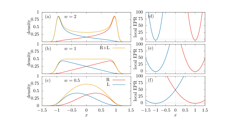
which shows that the local entropy production rate [29, 47] for right-moving particles is

$$\sigma_{\phi}(x)=\frac{1}{D}(w-kx)^{2}-k\,,$$ (22ak)

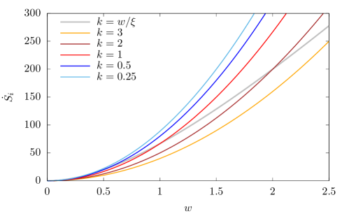
and $\sigma_{\psi}(x)=\sigma_{\phi}(-x)$ for left-moving particles, see figure 3. The local entropy production rate $\sigma_{\phi}$ is minimal at the characteristic point $\xi=w/k$, where a right-moving particle has a zero expected velocity because the self-propulsion equals the force exerted by the potential, and its motion is entirely due to the thermal noise. We can calculate (22aj) using the moments derived in Sec. 2.3. On the basis of Eqs. (22aa), the total stationary internal entropy production is

$$\dot{S}_{i}=\frac{\alpha w^{2}}{D(k+\alpha)}\,,$$ (22al)

see figure 4.

Figure 4: Stationary internal entropy production rate of an RnT particle in a harmonic potential as a function of $w$, Equation (22al), with $\alpha=2$, $D=0.01$, $\xi=1$ and varying $k$. The points where the grey line crosses the lines with $k=0.5$, $k=1$ and $k=2$ give $\dot{S}_{i}$ in the examples shown in figure 3.

4 Discussion and conclusions

In this paper we have used the Doi-Peliti framework to describe an RnT particle in a harmonic potential and calculate its entropy production (22al) and other observables (such as (22x), (22aa), (22bb), (22be), (22bg), (22bj), (22bm) and (22bq)) in closed form. The key result in Equation (22al) shows that the stationary internal entropy production of an RnT particle is proportional to that of a drift-diffusive particle in free space, where $\dot{S}_{i}=w^{2}/D$ [40]. In the presence of an external harmonic potential ($k>0$), the entropy production is always smaller than that of a free particle. If there is no tumbling ($\alpha=0$), then the system is an Ornstein-Uhlenbeck process, which is at equilibrium and therefore produces no entropy.

The positive entropy production rate implies the breaking of time symmetry whereby forward and backward trajectories are distinguishable [40]. This is visible in the trajectory of an RnT particle, such as in figure 1, where we can see that the particle runs fast when "going down" the potential and it slows down as it moves up the steep slope of the potential.

The present example of an RnT particle illustrates the power of field theories that capture the microscopic dynamics to deal with active systems. Since the large scale behaviour of an RnT particle is that of a diffusive particle, by studying an effective theory that captures the large scale only, we would obtain that the entropy production is zero, in contradiction with our result (22al).

Finally, deriving the Doi-Peliti field theory presents an important technical challenge. Due to the external harmonic potential, the action functional is semi-local both in real space and in Fourier space. Instead, to diagonalise the action we decomposed the fields in a basis of Hermite polynomials following the spirit of the harmonic oscillator [37].

Appendix A Hermite polynomials

The definition of Hermite polynomials [48] we use in this paper is

$$H_{n}\left(x\right)=(-1)^{n}\,\mathchoice{e^{\frac{x^{2}}{2}}}{\operatorname{exp}\!\left(\frac{x^{2}}{2}\right)}{\operatorname{exp}\!\left(\frac{x^{2}}{2}\right)}{\operatorname{exp}\!\left(\frac{x^{2}}{2}\right)}\,\frac{\text{d}^{n}}{\text{d}x^{n}}\left(\mathchoice{e^{-\frac{x^{2}}{2}}}{\operatorname{exp}\!\left(-\frac{x^{2}}{2}\right)}{\operatorname{exp}\!\left(-\frac{x^{2}}{2}\right)}{\operatorname{exp}\!\left(-\frac{x^{2}}{2}\right)}\right)\,,$$ (22am)

where $x\in\mathbb{R}$, $n\in\mathbb{N}\cup\{0\}$. Some of the properties of Hermite polynomials that we use are listed in the following [48].

Orthogonality:

Hermite polynomials are orthogonal with respect to the weight function $f(x)=\mathchoice{e^{-{x^{2}}/{2}}}{\operatorname{exp}\!\left(-{x^{2}}/{2}\right)}{\operatorname{exp}\!\left(-{x^{2}}/{2}\right)}{\operatorname{exp}\!\left(-{x^{2}}/{2}\right)}$,

$$\int_{-\infty}^{\infty}\mathchoice{\!\text{d}x\,}{\!\text{d}x\,}{\!\text{d}x\,}{\!\text{d}x\,}\mathchoice{e^{-\frac{x^{2}}{2}}}{\operatorname{exp}\!\left(-\frac{x^{2}}{2}\right)}{\operatorname{exp}\!\left(-\frac{x^{2}}{2}\right)}{\operatorname{exp}\!\left(-\frac{x^{2}}{2}\right)}H_{n}\left(x\right)H_{m}\left(x\right)=\sqrt{2\pi}\,n!\,\delta_{n,m}\,,$$ (22an)

where $\delta_{n,m}$ is the Kronecker delta.

Hermite’s differential equation:

Hermite polynomials $H_{n}\left(x\right)$ are eigenfunctions of the differential operator

$$H^{\prime\prime}-xH^{\prime}=-\mu H\,,$$ (22ao)

for non-negative integer eigenvalues $\mu_{n}=n$. Using this equation, we can show that the Hermite functions $u_{n}(x)=f(x/L)H_{n}\left(x/L\right)$ are solution to the eigenvalue problem $\mathcal{L}[u]=u^{\prime\prime}+(x\,u)^{\prime}/L^{2}=\lambda u$ in Sec. 2, Equation (7), with eigenvalues $\lambda_{n}=-n/L^{2}$ [49].

Recurrence relation:

Hermite polynomials satisfy the recurrence relation

$$H_{n+1}\left(x\right)=xH_{n}\left(x\right)-H_{n}^{\prime}(x)\,.$$ (22ap)

Mehler’s formula:

Hermite polynomials satisfy the following identity [48, 37],

$$\mathchoice{e^{-\frac{x^{2}}{2}}}{\operatorname{exp}\!\left(-\frac{x^{2}}{2}\right)}{\operatorname{exp}\!\left(-\frac{x^{2}}{2}\right)}{\operatorname{exp}\!\left(-\frac{x^{2}}{2}\right)}\sum_{n=0}^{\infty}\frac{s^{n}}{n!}H_{n}\left(x\right)H_{n}\left(y\right)=\frac{1}{\sqrt{1-s^{2}}}\mathchoice{e^{-\frac{(x-ys)^{2}}{2\left(1-s^{2}\right)}}}{\operatorname{exp}\!\left(-\frac{(x-ys)^{2}}{2\left(1-s^{2}\right)}\right)}{\operatorname{exp}\!\left(-\frac{(x-ys)^{2}}{2\left(1-s^{2}\right)}\right)}{\operatorname{exp}\!\left(-\frac{(x-ys)^{2}}{2\left(1-s^{2}\right)}\right)}\,.$$ (22aq)

Appendix B Some propagators in closed form

We list the propagators that we have used to calculate in the observables. Using the bare propagators in (15) and the interaction part of the action in (12b), we obtain the following propagators in real time,

$$\leavevmode\hbox to51.64pt{\vbox to17.32pt{\pgfpicture\makeatletter\hbox{\hskip 25.0461pt\lower-0.5pt\hbox to0.0pt{\pgfsys@beginscope\pgfsys@invoke{ }\definecolor{pgfstrokecolor}{rgb}{0,0,0}\pgfsys@color@rgb@stroke{0}{0}{0}\pgfsys@invoke{ }\pgfsys@color@rgb@fill{0}{0}{0}\pgfsys@invoke{ }\pgfsys@setlinewidth{0.4pt}\pgfsys@invoke{ }\nullfont\pgfsys@beginscope\pgfsys@invoke{ }\pgfsys@invoke{\lxSVG@closescope }\pgfsys@endscope\hbox to0.0pt{\pgfsys@beginscope\pgfsys@invoke{ }{{}}{ {}{{}}{} {}{}{}{}{{{}{}}}{}{}{{{}{}}}\pgfsys@beginscope\pgfsys@invoke{ }\pgfsys@setlinewidth{1.0pt}\pgfsys@invoke{ }\definecolor[named]{pgfstrokecolor}{rgb}{0,0,0}\pgfsys@color@gray@stroke{0}\pgfsys@invoke{ }{}\pgfsys@moveto{16.00467pt}{0.0pt}\pgfsys@lineto{-16.00467pt}{0.0pt}\pgfsys@stroke\pgfsys@invoke{ }\hbox{\hbox{\hbox{{\pgfsys@beginscope\pgfsys@invoke{ }{{}{}{{ {}{}}}{ {}{}} {{}{{}}}{{}{}}{}{{}{}} { }{{{{}}\pgfsys@beginscope\pgfsys@invoke{ }\pgfsys@transformcm{1.0}{0.0}{0.0}{1.0}{8.74847pt}{5.77745pt}\pgfsys@invoke{ }\hbox{{\definecolor{pgfstrokecolor}{rgb}{0,0,0}\pgfsys@color@rgb@stroke{0}{0}{0}\pgfsys@invoke{ }\pgfsys@color@rgb@fill{0}{0}{0}\pgfsys@invoke{ }\hbox{{${}_{m},t^{\prime}$}} }}\pgfsys@invoke{\lxSVG@closescope }\pgfsys@endscope}}} \pgfsys@invoke{\lxSVG@closescope }\pgfsys@endscope}}}\hbox{{\pgfsys@beginscope\pgfsys@invoke{ }{{}{}{{ {}{}}}{ {}{}} {{}{{}}}{{}{}}{}{{}{}} { }{{{{}}\pgfsys@beginscope\pgfsys@invoke{ }\pgfsys@transformcm{1.0}{0.0}{0.0}{1.0}{-21.71309pt}{5.77744pt}\pgfsys@invoke{ }\hbox{{\definecolor{pgfstrokecolor}{rgb}{0,0,0}\pgfsys@color@rgb@stroke{0}{0}{0}\pgfsys@invoke{ }\pgfsys@color@rgb@fill{0}{0}{0}\pgfsys@invoke{ }\hbox{{${}_{n},t$}} }}\pgfsys@invoke{\lxSVG@closescope }\pgfsys@endscope}}} \pgfsys@invoke{\lxSVG@closescope }\pgfsys@endscope}}} \pgfsys@invoke{\lxSVG@closescope }\pgfsys@endscope} \pgfsys@invoke{\lxSVG@closescope }\pgfsys@endscope{}{}{}\hss}\pgfsys@discardpath\pgfsys@invoke{\lxSVG@closescope }\pgfsys@endscope\hss}}\lxSVG@closescope\endpgfpicture}}\,\hat{=}\left\langle{\rho_{n}(t)\tilde{\rho}_{m}(t^{\prime})}\right\rangle_{0}=\delta_{n,m}L\mathchoice{e^{-mk(t-t^{\prime})}}{\operatorname{exp}\!\left(-mk(t-t^{\prime})\right)}{\operatorname{exp}\!\left(-mk(t-t^{\prime})\right)}{\operatorname{exp}\!\left(-mk(t-t^{\prime})\right)}\,, {}_{m},t^{\prime} {}_{n},t {}_{m},t^{\prime} {}_{n},t$$ (22ar)

$$\leavevmode\hbox to51.64pt{\vbox to18.74pt{\pgfpicture\makeatletter\hbox{\hskip 25.0461pt\lower-1.92264pt\hbox to0.0pt{\pgfsys@beginscope\pgfsys@invoke{ }\definecolor{pgfstrokecolor}{rgb}{0,0,0}\pgfsys@color@rgb@stroke{0}{0}{0}\pgfsys@invoke{ }\pgfsys@color@rgb@fill{0}{0}{0}\pgfsys@invoke{ }\pgfsys@setlinewidth{0.4pt}\pgfsys@invoke{ }\nullfont\pgfsys@beginscope\pgfsys@invoke{ }\pgfsys@invoke{\lxSVG@closescope }\pgfsys@endscope\hbox to0.0pt{\pgfsys@beginscope\pgfsys@invoke{ }{{}}{ {}{{}}{} {}{}{}{}{{{}{}}}{}{}{{{}{}}} {}{{}{}}{}{}{}{{}}{{}}{{}{}}{{}{}}{{{{}{}{{}} }}{{}} {}{}{} }{{{{}{}{{}} }}{{}} {{}{}{}{}} {{}{}{}{}} }{{{{}{}{{}} }}{{}} {{}{}{}{}} {{}{}{}{}} }{{{{}{}{{}} }}{{}} {{}{}{}{}} {{}{}{}{}} }{{{{}{}{{}} }}{{}} {{}{}{}{}} {{}{}{}{}} }{{{{}{}{{}} }}{{}} {{}{}{}{}} {{}{}{}{}} }{{{{}{}{{}} }}{{}} {{}{}{}{}} {{}{}{}{}} }{{{{}{}{{}} }}{{}} {{}{}{}{}} {{}{}{}{}} }{{{{}{}{{}} }}{{}} {{}{}{}{}} {{}{}{}{}} }{{{{}{}{{}} }}{{}} {{}{}{}{}} {{}{}{}{}} }{{{{}{}{{}} }}{{}} {{}{}{}{}} {{}{}{}{}} }{{{{}{}{{}} }}{{}} {{}{}{}{}} {{}{}{}{}} }{{{{}{}{{}} }}{{}} {{}} } \pgfsys@beginscope\pgfsys@invoke{ }\pgfsys@setlinewidth{1.0pt}\pgfsys@invoke{ }\definecolor[named]{pgfstrokecolor}{rgb}{0,0,0}\pgfsys@color@gray@stroke{0}\pgfsys@invoke{ }{}\pgfsys@moveto{16.00467pt}{0.0pt}\pgfsys@curveto{15.37967pt}{0.0pt}{15.06717pt}{-1.42264pt}{14.44217pt}{-1.42264pt}\pgfsys@curveto{13.98967pt}{-1.42264pt}{13.59969pt}{-0.7284pt}{13.19217pt}{0.0pt}\pgfsys@curveto{12.78467pt}{0.72838pt}{12.39467pt}{1.42264pt}{11.94217pt}{1.42264pt}\pgfsys@curveto{11.48967pt}{1.42264pt}{11.09969pt}{0.7284pt}{10.69217pt}{0.0pt}\pgfsys@curveto{10.28467pt}{-0.72838pt}{9.89467pt}{-1.42264pt}{9.44217pt}{-1.42264pt}\pgfsys@curveto{8.98967pt}{-1.42264pt}{8.59969pt}{-0.7284pt}{8.19217pt}{0.0pt}\pgfsys@curveto{7.78467pt}{0.72838pt}{7.39467pt}{1.42264pt}{6.94217pt}{1.42264pt}\pgfsys@curveto{6.48967pt}{1.42264pt}{6.09969pt}{0.7284pt}{5.69217pt}{0.0pt}\pgfsys@curveto{5.28467pt}{-0.72838pt}{4.89467pt}{-1.42264pt}{4.44217pt}{-1.42264pt}\pgfsys@curveto{3.98967pt}{-1.42264pt}{3.59969pt}{-0.7284pt}{3.19217pt}{0.0pt}\pgfsys@curveto{2.78467pt}{0.72838pt}{2.39467pt}{1.42264pt}{1.94217pt}{1.42264pt}\pgfsys@curveto{1.48967pt}{1.42264pt}{1.09969pt}{0.7284pt}{0.69217pt}{0.0pt}\pgfsys@curveto{0.28467pt}{-0.72838pt}{-0.10533pt}{-1.42264pt}{-0.55783pt}{-1.42264pt}\pgfsys@curveto{-1.01033pt}{-1.42264pt}{-1.40031pt}{-0.7284pt}{-1.80783pt}{0.0pt}\pgfsys@curveto{-2.21533pt}{0.72838pt}{-2.60533pt}{1.42264pt}{-3.05783pt}{1.42264pt}\pgfsys@curveto{-3.51033pt}{1.42264pt}{-3.90031pt}{0.7284pt}{-4.30783pt}{0.0pt}\pgfsys@curveto{-4.71533pt}{-0.72838pt}{-5.10533pt}{-1.42264pt}{-5.55783pt}{-1.42264pt}\pgfsys@curveto{-6.01033pt}{-1.42264pt}{-6.40031pt}{-0.7284pt}{-6.80783pt}{0.0pt}\pgfsys@curveto{-7.21533pt}{0.72838pt}{-7.60533pt}{1.42264pt}{-8.05783pt}{1.42264pt}\pgfsys@curveto{-8.51033pt}{1.42264pt}{-8.90031pt}{0.7284pt}{-9.30783pt}{0.0pt}\pgfsys@curveto{-9.71533pt}{-0.72838pt}{-10.10533pt}{-1.42264pt}{-10.55783pt}{-1.42264pt}\pgfsys@curveto{-11.01033pt}{-1.42264pt}{-11.40031pt}{-0.7284pt}{-11.80783pt}{0.0pt}\pgfsys@curveto{-12.21533pt}{0.72838pt}{-12.60533pt}{1.42264pt}{-13.05783pt}{1.42264pt}\pgfsys@lineto{-16.00467pt}{0.0pt}\pgfsys@stroke\pgfsys@invoke{ }\hbox{\hbox{\hbox{{\pgfsys@beginscope\pgfsys@invoke{ }{{}{}{{ {}{}}}{ {}{}} {{}{{}}}{{}{}}{}{{}{}} { }{{{{}}\pgfsys@beginscope\pgfsys@invoke{ }\pgfsys@transformcm{1.0}{0.0}{0.0}{1.0}{8.74847pt}{5.77745pt}\pgfsys@invoke{ }\hbox{{\definecolor{pgfstrokecolor}{rgb}{0,0,0}\pgfsys@color@rgb@stroke{0}{0}{0}\pgfsys@invoke{ }\pgfsys@color@rgb@fill{0}{0}{0}\pgfsys@invoke{ }\hbox{{${}_{m},t^{\prime}$}} }}\pgfsys@invoke{\lxSVG@closescope }\pgfsys@endscope}}} \pgfsys@invoke{\lxSVG@closescope }\pgfsys@endscope}}}\hbox{{\pgfsys@beginscope\pgfsys@invoke{ }{{}{}{{ {}{}}}{ {}{}} {{}{{}}}{{}{}}{}{{}{}} { }{{{{}}\pgfsys@beginscope\pgfsys@invoke{ }\pgfsys@transformcm{1.0}{0.0}{0.0}{1.0}{-21.71309pt}{5.77744pt}\pgfsys@invoke{ }\hbox{{\definecolor{pgfstrokecolor}{rgb}{0,0,0}\pgfsys@color@rgb@stroke{0}{0}{0}\pgfsys@invoke{ }\pgfsys@color@rgb@fill{0}{0}{0}\pgfsys@invoke{ }\hbox{{${}_{n},t$}} }}\pgfsys@invoke{\lxSVG@closescope }\pgfsys@endscope}}} \pgfsys@invoke{\lxSVG@closescope }\pgfsys@endscope}}} \pgfsys@invoke{\lxSVG@closescope }\pgfsys@endscope} \pgfsys@invoke{\lxSVG@closescope }\pgfsys@endscope{}{}{}\hss}\pgfsys@discardpath\pgfsys@invoke{\lxSVG@closescope }\pgfsys@endscope\hss}}\lxSVG@closescope\endpgfpicture}}\,\hat{=}\left\langle{\nu_{n}(t)\tilde{\nu}_{m}(t^{\prime})}\right\rangle_{0}=\delta_{n,m}L\mathchoice{e^{-\left(mk+\alpha\right)(t-t^{\prime})}}{\operatorname{exp}\!\left(-\left(mk+\alpha\right)(t-t^{\prime})\right)}{\operatorname{exp}\!\left(-\left(mk+\alpha\right)(t-t^{\prime})\right)}{\operatorname{exp}\!\left(-\left(mk+\alpha\right)(t-t^{\prime})\right)}\,, {}_{m},t^{\prime} {}_{n},t {}_{m},t^{\prime} {}_{n},t$$ (22as)

$$\leavevmode\hbox to51.64pt{\vbox to18.74pt{\pgfpicture\makeatletter\hbox{\hskip 25.0461pt\lower-1.92264pt\hbox to0.0pt{\pgfsys@beginscope\pgfsys@invoke{ }\definecolor{pgfstrokecolor}{rgb}{0,0,0}\pgfsys@color@rgb@stroke{0}{0}{0}\pgfsys@invoke{ }\pgfsys@color@rgb@fill{0}{0}{0}\pgfsys@invoke{ }\pgfsys@setlinewidth{0.4pt}\pgfsys@invoke{ }\nullfont\pgfsys@beginscope\pgfsys@invoke{ }\pgfsys@invoke{\lxSVG@closescope }\pgfsys@endscope\hbox to0.0pt{\pgfsys@beginscope\pgfsys@invoke{ }{{}}{ {}{{}}{} {}{}{}{}{{{}{}}}\pgfsys@beginscope\pgfsys@invoke{ }\pgfsys@setlinewidth{1.0pt}\pgfsys@invoke{ }\definecolor[named]{pgfstrokecolor}{rgb}{0,0,0}\pgfsys@color@gray@stroke{0}\pgfsys@invoke{ }{}\pgfsys@moveto{0.0pt}{0.0pt}\pgfsys@lineto{-16.00467pt}{0.0pt}\pgfsys@stroke\pgfsys@invoke{ }\hbox{\hbox{{\pgfsys@beginscope\pgfsys@invoke{ }{{}{}{{ {}{}}}{ {}{}} {{}{{}}}{{}{}}{}{{}{}} { }{{{{}}\pgfsys@beginscope\pgfsys@invoke{ }\pgfsys@transformcm{1.0}{0.0}{0.0}{1.0}{-21.71309pt}{5.77744pt}\pgfsys@invoke{ }\hbox{{\definecolor{pgfstrokecolor}{rgb}{0,0,0}\pgfsys@color@rgb@stroke{0}{0}{0}\pgfsys@invoke{ }\pgfsys@color@rgb@fill{0}{0}{0}\pgfsys@invoke{ }\hbox{{${}_{n},t$}} }}\pgfsys@invoke{\lxSVG@closescope }\pgfsys@endscope}}} \pgfsys@invoke{\lxSVG@closescope }\pgfsys@endscope}}} \pgfsys@invoke{\lxSVG@closescope }\pgfsys@endscope{}{{}}{} {}{}{}{}{{{}{}}} {}{{}{}}{}{}{}{{}}{{}}{{}{}}{{}{}}{{{{}{}{{}} }}{{}} {}{}{} }{{{{}{}{{}} }}{{}} {}{}{} }{{{{}{}{{}} }}{{}} {{}} } \pgfsys@beginscope\pgfsys@invoke{ }\pgfsys@setlinewidth{1.0pt}\pgfsys@invoke{ }\definecolor[named]{pgfstrokecolor}{rgb}{0,0,0}\pgfsys@color@gray@stroke{0}\pgfsys@invoke{ }{}\pgfsys@moveto{16.00467pt}{0.0pt}\pgfsys@curveto{15.37967pt}{0.0pt}{15.06717pt}{-1.42264pt}{14.44217pt}{-1.42264pt}\pgfsys@curveto{13.81717pt}{-1.42264pt}{13.50467pt}{0.0pt}{12.87967pt}{0.0pt}\pgfsys@lineto{0.0pt}{0.0pt}\pgfsys@stroke\pgfsys@invoke{ }\hbox{\hbox{{\pgfsys@beginscope\pgfsys@invoke{ }{{}{}{{ {}{}}}{ {}{}} {{}{{}}}{{}{}}{}{{}{}} { }{{{{}}\pgfsys@beginscope\pgfsys@invoke{ }\pgfsys@transformcm{1.0}{0.0}{0.0}{1.0}{8.74847pt}{5.77745pt}\pgfsys@invoke{ }\hbox{{\definecolor{pgfstrokecolor}{rgb}{0,0,0}\pgfsys@color@rgb@stroke{0}{0}{0}\pgfsys@invoke{ }\pgfsys@color@rgb@fill{0}{0}{0}\pgfsys@invoke{ }\hbox{{${}_{m},t^{\prime}$}} }}\pgfsys@invoke{\lxSVG@closescope }\pgfsys@endscope}}} \pgfsys@invoke{\lxSVG@closescope }\pgfsys@endscope}}} \pgfsys@invoke{\lxSVG@closescope }\pgfsys@endscope} \pgfsys@invoke{\lxSVG@closescope }\pgfsys@endscope{}{}{}\hss}\pgfsys@discardpath\pgfsys@invoke{\lxSVG@closescope }\pgfsys@endscope\hss}}\lxSVG@closescope\endpgfpicture}}\,\hat{=}\left\langle{\rho_{n}(t)\tilde{\nu}_{m}(t^{\prime})(-\mathcal{A}_{1})}\right\rangle_{0}=\delta_{n,m+1}\frac{w}{k-\alpha}\mathchoice{e^{-mk(t^{\prime}-t^{\prime})}}{\operatorname{exp}\!\left(-mk(t^{\prime}-t^{\prime})\right)}{\operatorname{exp}\!\left(-mk(t^{\prime}-t^{\prime})\right)}{\operatorname{exp}\!\left(-mk(t^{\prime}-t^{\prime})\right)}\left(\mathchoice{e^{-\alpha(t-t^{\prime})}}{\operatorname{exp}\!\left(-\alpha(t-t^{\prime})\right)}{\operatorname{exp}\!\left(-\alpha(t-t^{\prime})\right)}{\operatorname{exp}\!\left(-\alpha(t-t^{\prime})\right)}-\mathchoice{e^{-k(t-t^{\prime})}}{\operatorname{exp}\!\left(-k(t-t^{\prime})\right)}{\operatorname{exp}\!\left(-k(t-t^{\prime})\right)}{\operatorname{exp}\!\left(-k(t-t^{\prime})\right)}\right)\,, {}_{n},t {}_{m},t^{\prime} {}_{n},t {}_{m},t^{\prime}$$ (22at)

$$\leavevmode\hbox to51.64pt{\vbox to18.74pt{\pgfpicture\makeatletter\hbox{\hskip 25.0461pt\lower-1.92264pt\hbox to0.0pt{\pgfsys@beginscope\pgfsys@invoke{ }\definecolor{pgfstrokecolor}{rgb}{0,0,0}\pgfsys@color@rgb@stroke{0}{0}{0}\pgfsys@invoke{ }\pgfsys@color@rgb@fill{0}{0}{0}\pgfsys@invoke{ }\pgfsys@setlinewidth{0.4pt}\pgfsys@invoke{ }\nullfont\pgfsys@beginscope\pgfsys@invoke{ }\pgfsys@invoke{\lxSVG@closescope }\pgfsys@endscope\hbox to0.0pt{\pgfsys@beginscope\pgfsys@invoke{ }{{}}{ {}{{}}{} {}{}{}{}{{{}{}}} {}{{}{}}{}{}{}{{}}{{}}{{}{}}{{}{}}{{{{}{}{{}} }}{{}} {}{}{} }{{{{}{}{{}} }}{{}} {{}{}{}{}} {{}{}{}{}} }{{{{}{}{{}} }}{{}} {{}{}{}{}} {{}{}{}{}} }{{{{}{}{{}} }}{{}} {{}{}{}{}} {{}{}{}{}} }{{{{}{}{{}} }}{{}} {{}{}{}{}} {{}{}{}{}} }{{{{}{}{{}} }}{{}} {{}{}{}{}} {{}{}{}{}} }{{{{}{}{{}} }}{{}} {{}} } \pgfsys@beginscope\pgfsys@invoke{ }\pgfsys@setlinewidth{1.0pt}\pgfsys@invoke{ }\definecolor[named]{pgfstrokecolor}{rgb}{0,0,0}\pgfsys@color@gray@stroke{0}\pgfsys@invoke{ }{}\pgfsys@moveto{0.0pt}{0.0pt}\pgfsys@curveto{-0.625pt}{0.0pt}{-0.9375pt}{-1.42264pt}{-1.5625pt}{-1.42264pt}\pgfsys@curveto{-2.015pt}{-1.42264pt}{-2.40498pt}{-0.7284pt}{-2.8125pt}{0.0pt}\pgfsys@curveto{-3.22pt}{0.72838pt}{-3.61pt}{1.42264pt}{-4.0625pt}{1.42264pt}\pgfsys@curveto{-4.515pt}{1.42264pt}{-4.90498pt}{0.7284pt}{-5.3125pt}{0.0pt}\pgfsys@curveto{-5.72pt}{-0.72838pt}{-6.11pt}{-1.42264pt}{-6.5625pt}{-1.42264pt}\pgfsys@curveto{-7.015pt}{-1.42264pt}{-7.40498pt}{-0.7284pt}{-7.8125pt}{0.0pt}\pgfsys@curveto{-8.22pt}{0.72838pt}{-8.61pt}{1.42264pt}{-9.0625pt}{1.42264pt}\pgfsys@curveto{-9.515pt}{1.42264pt}{-9.90498pt}{0.7284pt}{-10.3125pt}{0.0pt}\pgfsys@curveto{-10.72pt}{-0.72838pt}{-11.11pt}{-1.42264pt}{-11.5625pt}{-1.42264pt}\pgfsys@curveto{-12.015pt}{-1.42264pt}{-12.40498pt}{-0.7284pt}{-12.8125pt}{0.0pt}\pgfsys@curveto{-13.22pt}{0.72838pt}{-13.61pt}{1.42264pt}{-14.0625pt}{1.42264pt}\pgfsys@lineto{-16.00467pt}{0.0pt}\pgfsys@stroke\pgfsys@invoke{ }\hbox{\hbox{{\pgfsys@beginscope\pgfsys@invoke{ }{{}{}{{ {}{}}}{ {}{}} {{}{{}}}{{}{}}{}{{}{}} { }{{{{}}\pgfsys@beginscope\pgfsys@invoke{ }\pgfsys@transformcm{1.0}{0.0}{0.0}{1.0}{-21.71309pt}{5.77744pt}\pgfsys@invoke{ }\hbox{{\definecolor{pgfstrokecolor}{rgb}{0,0,0}\pgfsys@color@rgb@stroke{0}{0}{0}\pgfsys@invoke{ }\pgfsys@color@rgb@fill{0}{0}{0}\pgfsys@invoke{ }\hbox{{${}_{n},t$}} }}\pgfsys@invoke{\lxSVG@closescope }\pgfsys@endscope}}} \pgfsys@invoke{\lxSVG@closescope }\pgfsys@endscope}}} \pgfsys@invoke{\lxSVG@closescope }\pgfsys@endscope{}{{}}{} {}{}{}{}{{{}{}}}\pgfsys@beginscope\pgfsys@invoke{ }\pgfsys@setlinewidth{1.0pt}\pgfsys@invoke{ }\definecolor[named]{pgfstrokecolor}{rgb}{0,0,0}\pgfsys@color@gray@stroke{0}\pgfsys@invoke{ }{}\pgfsys@moveto{16.00467pt}{0.0pt}\pgfsys@lineto{0.0pt}{0.0pt}\pgfsys@stroke\pgfsys@invoke{ }\hbox{\hbox{{\pgfsys@beginscope\pgfsys@invoke{ }{{}{}{{ {}{}}}{ {}{}} {{}{{}}}{{}{}}{}{{}{}} { }{{{{}}\pgfsys@beginscope\pgfsys@invoke{ }\pgfsys@transformcm{1.0}{0.0}{0.0}{1.0}{8.74847pt}{5.77745pt}\pgfsys@invoke{ }\hbox{{\definecolor{pgfstrokecolor}{rgb}{0,0,0}\pgfsys@color@rgb@stroke{0}{0}{0}\pgfsys@invoke{ }\pgfsys@color@rgb@fill{0}{0}{0}\pgfsys@invoke{ }\hbox{{${}_{m},t^{\prime}$}} }}\pgfsys@invoke{\lxSVG@closescope }\pgfsys@endscope}}} \pgfsys@invoke{\lxSVG@closescope }\pgfsys@endscope}}} \pgfsys@invoke{\lxSVG@closescope }\pgfsys@endscope} \pgfsys@invoke{\lxSVG@closescope }\pgfsys@endscope{}{}{}\hss}\pgfsys@discardpath\pgfsys@invoke{\lxSVG@closescope }\pgfsys@endscope\hss}}\lxSVG@closescope\endpgfpicture}}\,\hat{=}\left\langle{\nu_{n}(t)\tilde{\rho}_{m}(t^{\prime})(-\mathcal{A}_{1})}\right\rangle_{0}=\delta_{n,m+1}\frac{w}{k+\alpha}\mathchoice{e^{-mk(t^{\prime}-t^{\prime})}}{\operatorname{exp}\!\left(-mk(t^{\prime}-t^{\prime})\right)}{\operatorname{exp}\!\left(-mk(t^{\prime}-t^{\prime})\right)}{\operatorname{exp}\!\left(-mk(t^{\prime}-t^{\prime})\right)}\left(1-\mathchoice{e^{-(k+\alpha)(t^{\prime}-t^{\prime})}}{\operatorname{exp}\!\left(-(k+\alpha)(t^{\prime}-t^{\prime})\right)}{\operatorname{exp}\!\left(-(k+\alpha)(t^{\prime}-t^{\prime})\right)}{\operatorname{exp}\!\left(-(k+\alpha)(t^{\prime}-t^{\prime})\right)}\right)\,, {}_{n},t {}_{m},t^{\prime} {}_{n},t {}_{m},t^{\prime}$$ (22au)

$$\leavevmode\hbox to51.64pt{\vbox to18.74pt{\pgfpicture\makeatletter\hbox{\hskip 25.0461pt\lower-1.92264pt\hbox to0.0pt{\pgfsys@beginscope\pgfsys@invoke{ }\definecolor{pgfstrokecolor}{rgb}{0,0,0}\pgfsys@color@rgb@stroke{0}{0}{0}\pgfsys@invoke{ }\pgfsys@color@rgb@fill{0}{0}{0}\pgfsys@invoke{ }\pgfsys@setlinewidth{0.4pt}\pgfsys@invoke{ }\nullfont\pgfsys@beginscope\pgfsys@invoke{ }\pgfsys@invoke{\lxSVG@closescope }\pgfsys@endscope\hbox to0.0pt{\pgfsys@beginscope\pgfsys@invoke{ }{{}}{ {}{{}}{} {}{}{}{}{{{}{}}}\pgfsys@beginscope\pgfsys@invoke{ }\pgfsys@setlinewidth{1.0pt}\pgfsys@invoke{ }\definecolor[named]{pgfstrokecolor}{rgb}{0,0,0}\pgfsys@color@gray@stroke{0}\pgfsys@invoke{ }{}\pgfsys@moveto{-6.40192pt}{0.0pt}\pgfsys@lineto{-16.00467pt}{0.0pt}\pgfsys@stroke\pgfsys@invoke{ }\hbox{\hbox{{\pgfsys@beginscope\pgfsys@invoke{ }{{}{}{{ {}{}}}{ {}{}} {{}{{}}}{{}{}}{}{{}{}} { }{{{{}}\pgfsys@beginscope\pgfsys@invoke{ }\pgfsys@transformcm{1.0}{0.0}{0.0}{1.0}{-21.71309pt}{5.77744pt}\pgfsys@invoke{ }\hbox{{\definecolor{pgfstrokecolor}{rgb}{0,0,0}\pgfsys@color@rgb@stroke{0}{0}{0}\pgfsys@invoke{ }\pgfsys@color@rgb@fill{0}{0}{0}\pgfsys@invoke{ }\hbox{{${}_{n},t$}} }}\pgfsys@invoke{\lxSVG@closescope }\pgfsys@endscope}}} \pgfsys@invoke{\lxSVG@closescope }\pgfsys@endscope}}} \pgfsys@invoke{\lxSVG@closescope }\pgfsys@endscope{}{{}}{} {}{} {}{{}{}}{}{}{}{{}}{{}}{{}{}}{{}{}}{{{{}{}{{}} }}{{}} {}{}{} }{{{{}{}{{}} }}{{}} {{}{}{}{}} {{}{}{}{}} }{{{{}{}{{}} }}{{}} {{}{}{}{}} {{}{}{}{}} }{{{{}{}{{}} }}{{}} {{}{}{}{}} {{}{}{}{}} }{{{{}{}{{}} }}{{}} {{}} } \pgfsys@beginscope\pgfsys@invoke{ }\pgfsys@setlinewidth{1.0pt}\pgfsys@invoke{ }\definecolor[named]{pgfstrokecolor}{rgb}{0,0,0}\pgfsys@color@gray@stroke{0}\pgfsys@invoke{ }{}\pgfsys@moveto{6.40192pt}{0.0pt}\pgfsys@curveto{5.77692pt}{0.0pt}{5.46442pt}{-1.42264pt}{4.83942pt}{-1.42264pt}\pgfsys@curveto{4.38692pt}{-1.42264pt}{3.99693pt}{-0.7284pt}{3.58942pt}{0.0pt}\pgfsys@curveto{3.18192pt}{0.72838pt}{2.79192pt}{1.42264pt}{2.33942pt}{1.42264pt}\pgfsys@curveto{1.88692pt}{1.42264pt}{1.49693pt}{0.7284pt}{1.08942pt}{0.0pt}\pgfsys@curveto{0.68192pt}{-0.72838pt}{0.29192pt}{-1.42264pt}{-0.16058pt}{-1.42264pt}\pgfsys@curveto{-0.61308pt}{-1.42264pt}{-1.00307pt}{-0.7284pt}{-1.41058pt}{0.0pt}\pgfsys@curveto{-1.81808pt}{0.72838pt}{-2.20808pt}{1.42264pt}{-2.66058pt}{1.42264pt}\pgfsys@lineto{-6.40192pt}{0.0pt}\pgfsys@stroke\pgfsys@invoke{ } \pgfsys@invoke{\lxSVG@closescope }\pgfsys@endscope{}{{}}{} {}{}{}{}{{{}{}}}\pgfsys@beginscope\pgfsys@invoke{ }\pgfsys@setlinewidth{1.0pt}\pgfsys@invoke{ }\definecolor[named]{pgfstrokecolor}{rgb}{0,0,0}\pgfsys@color@gray@stroke{0}\pgfsys@invoke{ }{}\pgfsys@moveto{16.00467pt}{0.0pt}\pgfsys@lineto{6.40192pt}{0.0pt}\pgfsys@stroke\pgfsys@invoke{ }\hbox{\hbox{{\pgfsys@beginscope\pgfsys@invoke{ }{{}{}{{ {}{}}}{ {}{}} {{}{{}}}{{}{}}{}{{}{}} { }{{{{}}\pgfsys@beginscope\pgfsys@invoke{ }\pgfsys@transformcm{1.0}{0.0}{0.0}{1.0}{8.74847pt}{5.77745pt}\pgfsys@invoke{ }\hbox{{\definecolor{pgfstrokecolor}{rgb}{0,0,0}\pgfsys@color@rgb@stroke{0}{0}{0}\pgfsys@invoke{ }\pgfsys@color@rgb@fill{0}{0}{0}\pgfsys@invoke{ }\hbox{{${}_{m},t^{\prime}$}} }}\pgfsys@invoke{\lxSVG@closescope }\pgfsys@endscope}}} \pgfsys@invoke{\lxSVG@closescope }\pgfsys@endscope}}} \pgfsys@invoke{\lxSVG@closescope }\pgfsys@endscope} \pgfsys@invoke{\lxSVG@closescope }\pgfsys@endscope{}{}{}\hss}\pgfsys@discardpath\pgfsys@invoke{\lxSVG@closescope }\pgfsys@endscope\hss}}\lxSVG@closescope\endpgfpicture}}\,\hat{=}\left\langle{\rho_{n}(t)\tilde{\rho}_{m}(t^{\prime})(-\mathcal{A}_{1})^{2}}\right\rangle_{0} {}_{n},t {}_{m},t^{\prime} {}_{n},t {}_{m},t^{\prime}$$

$$=\delta_{n,m+2}\frac{w^{2}}{L}\mathchoice{e^{-mk(t-t^{\prime})}}{\operatorname{exp}\!\left(-mk(t-t^{\prime})\right)}{\operatorname{exp}\!\left(-mk(t-t^{\prime})\right)}{\operatorname{exp}\!\left(-mk(t-t^{\prime})\right)}\left(\frac{e^{-2k(t-t^{\prime})}}{2k(k-\alpha)}+\frac{e^{-(k+\alpha)(t-t^{\prime})}}{(k+\alpha)(\alpha-k)}+\frac{1}{2k(k+\alpha)}\right)\,,$$ (22av)

$$\leavevmode\hbox to51.64pt{\vbox to18.74pt{\pgfpicture\makeatletter\hbox{\hskip 25.0461pt\lower-1.92264pt\hbox to0.0pt{\pgfsys@beginscope\pgfsys@invoke{ }\definecolor{pgfstrokecolor}{rgb}{0,0,0}\pgfsys@color@rgb@stroke{0}{0}{0}\pgfsys@invoke{ }\pgfsys@color@rgb@fill{0}{0}{0}\pgfsys@invoke{ }\pgfsys@setlinewidth{0.4pt}\pgfsys@invoke{ }\nullfont\pgfsys@beginscope\pgfsys@invoke{ }\pgfsys@invoke{\lxSVG@closescope }\pgfsys@endscope\hbox to0.0pt{\pgfsys@beginscope\pgfsys@invoke{ }{{}}{ {}{{}}{} {}{}{}{}{{{}{}}} {}{{}{}}{}{}{}{{}}{{}}{{}{}}{{}{}}{{{{}{}{{}} }}{{}} {}{}{} }{{{{}{}{{}} }}{{}} {{}{}{}{}} {{}{}{}{}} }{{{{}{}{{}} }}{{}} {{}{}{}{}} {{}{}{}{}} }{{{{}{}{{}} }}{{}} {{}{}{}{}} {{}{}{}{}} }{{{{}{}{{}} }}{{}} {{}} } \pgfsys@beginscope\pgfsys@invoke{ }\pgfsys@setlinewidth{1.0pt}\pgfsys@invoke{ }\definecolor[named]{pgfstrokecolor}{rgb}{0,0,0}\pgfsys@color@gray@stroke{0}\pgfsys@invoke{ }{}\pgfsys@moveto{-3.20079pt}{0.0pt}\pgfsys@curveto{-3.82579pt}{0.0pt}{-4.13829pt}{-1.42264pt}{-4.76329pt}{-1.42264pt}\pgfsys@curveto{-5.21579pt}{-1.42264pt}{-5.60577pt}{-0.7284pt}{-6.01329pt}{0.0pt}\pgfsys@curveto{-6.42079pt}{0.72838pt}{-6.81079pt}{1.42264pt}{-7.26329pt}{1.42264pt}\pgfsys@curveto{-7.71579pt}{1.42264pt}{-8.10577pt}{0.7284pt}{-8.51329pt}{0.0pt}\pgfsys@curveto{-8.92079pt}{-0.72838pt}{-9.31079pt}{-1.42264pt}{-9.76329pt}{-1.42264pt}\pgfsys@curveto{-10.21579pt}{-1.42264pt}{-10.60577pt}{-0.7284pt}{-11.01329pt}{0.0pt}\pgfsys@curveto{-11.42079pt}{0.72838pt}{-11.81079pt}{1.42264pt}{-12.26329pt}{1.42264pt}\pgfsys@lineto{-16.00467pt}{0.0pt}\pgfsys@stroke\pgfsys@invoke{ }\hbox{\hbox{{\pgfsys@beginscope\pgfsys@invoke{ }{{}{}{{ {}{}}}{ {}{}} {{}{{}}}{{}{}}{}{{}{}} { }{{{{}}\pgfsys@beginscope\pgfsys@invoke{ }\pgfsys@transformcm{1.0}{0.0}{0.0}{1.0}{-21.71309pt}{5.77744pt}\pgfsys@invoke{ }\hbox{{\definecolor{pgfstrokecolor}{rgb}{0,0,0}\pgfsys@color@rgb@stroke{0}{0}{0}\pgfsys@invoke{ }\pgfsys@color@rgb@fill{0}{0}{0}\pgfsys@invoke{ }\hbox{{${}_{n},t$}} }}\pgfsys@invoke{\lxSVG@closescope }\pgfsys@endscope}}} \pgfsys@invoke{\lxSVG@closescope }\pgfsys@endscope}}} \pgfsys@invoke{\lxSVG@closescope }\pgfsys@endscope{}{{}}{} {}{}\pgfsys@beginscope\pgfsys@invoke{ }\pgfsys@setlinewidth{1.0pt}\pgfsys@invoke{ }\definecolor[named]{pgfstrokecolor}{rgb}{0,0,0}\pgfsys@color@gray@stroke{0}\pgfsys@invoke{ }{}\pgfsys@moveto{3.20079pt}{0.0pt}\pgfsys@lineto{-3.20079pt}{0.0pt}\pgfsys@stroke\pgfsys@invoke{ } \pgfsys@invoke{\lxSVG@closescope }\pgfsys@endscope{}{{}}{} {}{}{}{}{{{}{}}} {}{{}{}}{}{}{}{{}}{{}}{{}{}}{{}{}}{{{{}{}{{}} }}{{}} {}{}{} }{{{{}{}{{}} }}{{}} {}{}{} }{{{{}{}{{}} }}{{}} {{}} } \pgfsys@beginscope\pgfsys@invoke{ }\pgfsys@setlinewidth{1.0pt}\pgfsys@invoke{ }\definecolor[named]{pgfstrokecolor}{rgb}{0,0,0}\pgfsys@color@gray@stroke{0}\pgfsys@invoke{ }{}\pgfsys@moveto{16.00467pt}{0.0pt}\pgfsys@curveto{15.37967pt}{0.0pt}{15.06717pt}{-1.42264pt}{14.44217pt}{-1.42264pt}\pgfsys@curveto{13.81717pt}{-1.42264pt}{13.50467pt}{0.0pt}{12.87967pt}{0.0pt}\pgfsys@lineto{3.20079pt}{0.0pt}\pgfsys@stroke\pgfsys@invoke{ }\hbox{\hbox{{\pgfsys@beginscope\pgfsys@invoke{ }{{}{}{{ {}{}}}{ {}{}} {{}{{}}}{{}{}}{}{{}{}} { }{{{{}}\pgfsys@beginscope\pgfsys@invoke{ }\pgfsys@transformcm{1.0}{0.0}{0.0}{1.0}{8.74847pt}{5.77745pt}\pgfsys@invoke{ }\hbox{{\definecolor{pgfstrokecolor}{rgb}{0,0,0}\pgfsys@color@rgb@stroke{0}{0}{0}\pgfsys@invoke{ }\pgfsys@color@rgb@fill{0}{0}{0}\pgfsys@invoke{ }\hbox{{${}_{m},t^{\prime}$}} }}\pgfsys@invoke{\lxSVG@closescope }\pgfsys@endscope}}} \pgfsys@invoke{\lxSVG@closescope }\pgfsys@endscope}}} \pgfsys@invoke{\lxSVG@closescope }\pgfsys@endscope} \pgfsys@invoke{\lxSVG@closescope }\pgfsys@endscope{}{}{}\hss}\pgfsys@discardpath\pgfsys@invoke{\lxSVG@closescope }\pgfsys@endscope\hss}}\lxSVG@closescope\endpgfpicture}}\,\hat{=}\left\langle{\nu_{n}(t)\tilde{\nu}_{m}(t^{\prime})(-\mathcal{A}_{1})^{2}}\right\rangle_{0} {}_{n},t {}_{m},t^{\prime} {}_{n},t {}_{m},t^{\prime}$$

$$=\delta_{n,m+2}\frac{w^{2}}{L}\mathchoice{e^{-mk(t-t^{\prime})}}{\operatorname{exp}\!\left(-mk(t-t^{\prime})\right)}{\operatorname{exp}\!\left(-mk(t-t^{\prime})\right)}{\operatorname{exp}\!\left(-mk(t-t^{\prime})\right)}\left(\frac{e^{-(2k+\alpha)(t-t^{\prime})}}{2k(k+\alpha)}+\frac{e^{-k(t-t^{\prime})}}{(k+\alpha)(\alpha-k)}+\frac{e^{-\alpha(t-t^{\prime})}}{2k(k-\alpha)}\right)\,,$$ (22aw)

after letting $r\to 0$. These propagators are then used to calculate the full propagator in real space via

$$\langle{\rho(x,t)\widetilde{\rho}(x^{\prime},t^{\prime})}\rangle=\frac{1}{L^{2}}\sum_{n,m,N}u_{n}(x)\widetilde{u}_{m}(x^{\prime})\frac{1}{N!}\left\langle{\rho_{n}(t)\widetilde{\rho}_{m}(t^{\prime})(-\mathcal{A}_{1})^{N}}\right\rangle_{0}\,,$$ (22ax)

where $\mathord{\mathop{\rho}\limits^{\scriptscriptstyle(\sim)}}$ may be replaced by $\mathord{\mathop{\nu}\limits^{\scriptscriptstyle(\sim)}}$. The stationary distribution is derived from this expression in G.

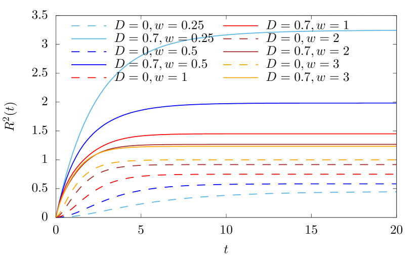
Appendix C Mean square displacement

The mean square displacement is defined as

$$R^{2}(t)=\left\langle{\left(x(t)-x_{0}\right)^{2}}\right\rangle\,.$$ (22ay)

Assuming that the system is initialised with a right-moving particle, the propagator that probes for any particle at a later time is $\big{\langle}{\big{(}\phi(x,t)+\psi(x,t)\big{)}\widetilde{\phi}(x_{0},0)}\big{\rangle}$. Following the same scheme as in Sec. 2.3, the first and second moments of the position of an RnT particle are

$$\left\langle{x(t)}\right\rangle=x_{0}\mathchoice{e^{-kt}}{\operatorname{exp}\!\left(-kt\right)}{\operatorname{exp}\!\left(-kt\right)}{\operatorname{exp}\!\left(-kt\right)}+\frac{w}{k-\alpha}\left(\mathchoice{e^{-\alpha t}}{\operatorname{exp}\!\left(-\alpha t\right)}{\operatorname{exp}\!\left(-\alpha t\right)}{\operatorname{exp}\!\left(-\alpha t\right)}-\mathchoice{e^{-kt}}{\operatorname{exp}\!\left(-kt\right)}{\operatorname{exp}\!\left(-kt\right)}{\operatorname{exp}\!\left(-kt\right)}\right)\,,$$ (22az)

$$\left\langle{x^{2}(t)}\right\rangle=x_{0}^{2}\mathchoice{e^{-2kt}}{\operatorname{exp}\!\left(-2kt\right)}{\operatorname{exp}\!\left(-2kt\right)}{\operatorname{exp}\!\left(-2kt\right)}+\frac{D}{k}\left(1-\mathchoice{e^{-2kt}}{\operatorname{exp}\!\left(-2kt\right)}{\operatorname{exp}\!\left(-2kt\right)}{\operatorname{exp}\!\left(-2kt\right)}\right)+2\frac{x_{0}w}{k-\alpha}\left(\mathchoice{e^{-(k+\alpha)t}}{\operatorname{exp}\!\left(-(k+\alpha)t\right)}{\operatorname{exp}\!\left(-(k+\alpha)t\right)}{\operatorname{exp}\!\left(-(k+\alpha)t\right)}-\mathchoice{e^{-2kt}}{\operatorname{exp}\!\left(-2kt\right)}{\operatorname{exp}\!\left(-2kt\right)}{\operatorname{exp}\!\left(-2kt\right)}\right)$$

$$\qquad+2w^{2}\left(\frac{\mathchoice{e^{-2kt}}{\operatorname{exp}\!\left(-2kt\right)}{\operatorname{exp}\!\left(-2kt\right)}{\operatorname{exp}\!\left(-2kt\right)}}{2k(k-\alpha)}+\frac{\mathchoice{e^{-(k+\alpha)t}}{\operatorname{exp}\!\left(-(k+\alpha)t\right)}{\operatorname{exp}\!\left(-(k+\alpha)t\right)}{\operatorname{exp}\!\left(-(k+\alpha)t\right)}}{(k+\alpha)(\alpha-k)}+\frac{1}{2k(k+\alpha)}\right)\,.$$ (22ba)

Then, the mean square displacement at stationarity is

$$\lim_{t\to\infty}R^{2}(t)=x_{0}^{2}+\frac{D}{k}+\frac{w^{2}}{k(k+\alpha)}\,,$$ (22bb)

see figure 5(a).

(a)

(b)

Figure 5: (5(a)) Mean square displacement $R^{2}(t)$ and (5(b)) expected velocity $\left\langle{\mathcal{W}_{\phi}(t)}\right\rangle$ of an RnT particle in a harmonic potential. In (5(a)), $x_{0}=0.5$, $\alpha=1$, $k=w/\xi$ with $\xi=1$, and a range of $D$, using Eqs. (22ay), (22az) and (22ba). In (5(b)), $k=0.5$, $\alpha=1$ and a range of $x_{0}$ and $w$, using Eqs. (22bd), (22za) and (22zb). The dotted lines show the particle’s self-propulsion speeds $w$, which are the instantaneous velocities at the origin.

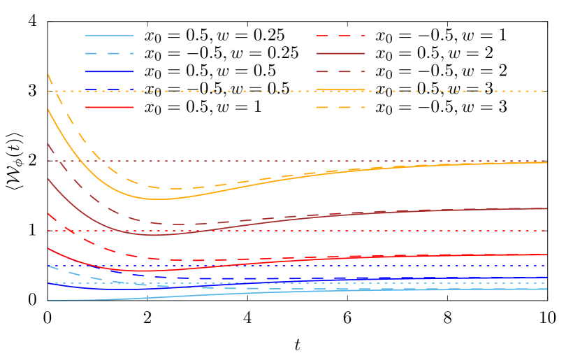
Appendix D Expected velocity

To calculate the expected velocity of a right-moving particle, one could naïvely differentiate the expected position $\left\langle{x_{\phi}(t)}\right\rangle$ in Equation (22zb) with respect to time,

$$\partial_{t}\left\langle{x_{\phi}(t)}\right\rangle=\int\mathchoice{\!\text{d}x\,}{\!\text{d}x\,}{\!\text{d}x\,}{\!\text{d}x\,}x\,\partial_{t}P_{\phi}(x,t)\,.$$ (22bc)

However, this expression fails to capture the expected velocity because in the limit $t\to\infty$, the stationary distribution satisfies $\partial_{t}P_{\phi}(x,t)=0$, implying that the result in (22bc) is zero. This is in contradiction with the nature of an RnT particle, which has a perpetual non-zero drift. Ultimately, the ambiguity in the definition of the velocity is a matter of Ito versus Stratonovich, namely to consider a particle’s displacement conditional to its point of departure (Ito), its point of arrival or the average of the two (Stratonovich).

Instead, to calculate the expected velocity of a right-moving particle $\left\langle{\mathcal{W}_{\phi}(t)}\right\rangle$ we draw on its local velocity, which is $w-kx$ given its position $x$ prior to its instantaneous departure, as captured by the Fokker-Planck Equation (3a). The expected velocity is then the conditional expectation

$$\left\langle{\mathcal{W}_{\phi}(t)}\right\rangle=\frac{\int\mathchoice{\!\text{d}x\,}{\!\text{d}x\,}{\!\text{d}x\,}{\!\text{d}x\,}(w-kx)\langle{\phi(x,t)\widetilde{\phi}(x_{0},t_{0})}\rangle}{\int\mathchoice{\!\text{d}x^{\prime}\,}{\!\text{d}x^{\prime}\,}{\!\text{d}x^{\prime}\,}{\!\text{d}x^{\prime}\,}\langle{\phi(x^{\prime},t)\widetilde{\phi}(x_{0},t_{0})}\rangle}\,,$$ (22bd)

which, using Eqs. (22za) and (22zb), is, at stationarity

$$\lim_{t\to\infty}\left\langle{\mathcal{W}_{\phi}(t)}\right\rangle=\frac{\alpha w}{k+\alpha}\,,$$ (22be)

see figure 5(b).

Appendix E Two-point correlation function

The two-point correlation function $\mathcal{F}(x,y;t)$ is the observable

$$\mathcal{F}(x,y;t)=\big{\langle}{\big{(}\phi(x,t)+\psi(x,t)\big{)}\big{(}\phi(y,t)+\psi(y,t)\big{)}\widetilde{\phi}(x_{0},0)}\big{\rangle}+\big{\langle}{\big{(}\phi(x,t)+\psi(x,t)\big{)}\widetilde{\phi}(x_{0},0)}\big{\rangle}\delta(x-y)\,,$$ (22bf)

where, after placing a right-moving particle at $x_{0}$ at time $t_{0}$, the system is probed for any particle at positions $x$ and $y$ simultaneously. The second term contributing only when $x=y$ has its origin in the commutation relation of the creation and annihilation operators [33]. Since there is exactly one RnT particle in the system, it cannot be in two different positions at the same time and therefore $\mathcal{F}(x,y;t)=0$ for all $t$ when $x\neq y$. Diagrammatically, (22bf) may be written as

$$\mathcal{F}(x,y;t)\hat{=}\sqrt{2}\left(\leavevmode\hbox to43.68pt{\vbox to14.63pt{\pgfpicture\makeatletter\hbox{\hskip 21.83957pt\lower-7.31319pt\hbox to0.0pt{\pgfsys@beginscope\pgfsys@invoke{ }\definecolor{pgfstrokecolor}{rgb}{0,0,0}\pgfsys@color@rgb@stroke{0}{0}{0}\pgfsys@invoke{ }\pgfsys@color@rgb@fill{0}{0}{0}\pgfsys@invoke{ }\pgfsys@setlinewidth{0.4pt}\pgfsys@invoke{ }\nullfont\pgfsys@beginscope\pgfsys@invoke{ }\pgfsys@invoke{\lxSVG@closescope }\pgfsys@endscope\hbox to0.0pt{\pgfsys@beginscope\pgfsys@invoke{ }{ {}{{}}{} {}{}\pgfsys@beginscope\pgfsys@invoke{ }\pgfsys@setlinewidth{1.0pt}\pgfsys@invoke{ }\definecolor[named]{pgfstrokecolor}{rgb}{0,0,0}\pgfsys@color@gray@stroke{0}\pgfsys@invoke{ }{}\pgfsys@moveto{-5.69046pt}{4.26773pt}\pgfsys@lineto{-21.33957pt}{4.26773pt}\pgfsys@stroke\pgfsys@invoke{ } \pgfsys@invoke{\lxSVG@closescope }\pgfsys@endscope{}{{}}{} {}{}\pgfsys@beginscope\pgfsys@invoke{ }\pgfsys@setlinewidth{1.0pt}\pgfsys@invoke{ }\definecolor[named]{pgfstrokecolor}{rgb}{0,0,0}\pgfsys@color@gray@stroke{0}\pgfsys@invoke{ }{}\pgfsys@moveto{-5.69046pt}{-4.26773pt}\pgfsys@lineto{-21.33957pt}{-4.26773pt}\pgfsys@stroke\pgfsys@invoke{ } \pgfsys@invoke{\lxSVG@closescope }\pgfsys@endscope{}{{}}{} {}{}\pgfsys@beginscope\pgfsys@invoke{ }\pgfsys@setlinewidth{1.0pt}\pgfsys@invoke{ }\definecolor[named]{pgfstrokecolor}{rgb}{0,0,0}\pgfsys@color@gray@stroke{0}\pgfsys@invoke{ }{}\pgfsys@moveto{21.33957pt}{0.0pt}\pgfsys@lineto{5.69046pt}{0.0pt}\pgfsys@stroke\pgfsys@invoke{ } \pgfsys@invoke{\lxSVG@closescope }\pgfsys@endscope{}{{}}{}{{{}} {}{}{}{}{}{}{}{} }\pgfsys@beginscope\pgfsys@invoke{ }\definecolor[named]{pgffillcolor}{rgb}{1,1,1}\pgfsys@color@gray@fill{1}\pgfsys@invoke{ }{}\pgfsys@moveto{0.0pt}{0.0pt}\pgfsys@moveto{7.11319pt}{0.0pt}\pgfsys@curveto{7.11319pt}{3.92854pt}{3.92854pt}{7.11319pt}{0.0pt}{7.11319pt}\pgfsys@curveto{-3.92854pt}{7.11319pt}{-7.11319pt}{3.92854pt}{-7.11319pt}{0.0pt}\pgfsys@curveto{-7.11319pt}{-3.92854pt}{-3.92854pt}{-7.11319pt}{0.0pt}{-7.11319pt}\pgfsys@curveto{3.92854pt}{-7.11319pt}{7.11319pt}{-3.92854pt}{7.11319pt}{0.0pt}\pgfsys@closepath\pgfsys@moveto{0.0pt}{0.0pt}\pgfsys@fillstroke\pgfsys@invoke{ } \pgfsys@invoke{\lxSVG@closescope }\pgfsys@endscope{}{{}}{}{{{}} {}{}{}{}{}{}{}{} }\pgfsys@beginscope\pgfsys@invoke{ }\pgfsys@invoke{ }{0.0}{1.0}{0.0pt}{0.0pt}{ \lxSVG@closescope }{0}\definecolor[named]{pgf@tempcolor}{rgb}{0,0,0}\pgfsys@invoke{\lxSVG@setpatternuncolored@{3}{0}{0}{0} }{}\pgfsys@moveto{0.0pt}{0.0pt}\pgfsys@moveto{7.11319pt}{0.0pt}\pgfsys@curveto{7.11319pt}{3.92854pt}{3.92854pt}{7.11319pt}{0.0pt}{7.11319pt}\pgfsys@curveto{-3.92854pt}{7.11319pt}{-7.11319pt}{3.92854pt}{-7.11319pt}{0.0pt}\pgfsys@curveto{-7.11319pt}{-3.92854pt}{-3.92854pt}{-7.11319pt}{0.0pt}{-7.11319pt}\pgfsys@curveto{3.92854pt}{-7.11319pt}{7.11319pt}{-3.92854pt}{7.11319pt}{0.0pt}\pgfsys@closepath\pgfsys@moveto{0.0pt}{0.0pt}\pgfsys@fillstroke\pgfsys@invoke{ } \pgfsys@invoke{\lxSVG@closescope }\pgfsys@endscope} \pgfsys@invoke{\lxSVG@closescope }\pgfsys@endscope{}{}{}\hss}\pgfsys@discardpath\pgfsys@invoke{\lxSVG@closescope }\pgfsys@endscope\hss}}\lxSVG@closescope\endpgfpicture}}+\leavevmode\hbox to43.68pt{\vbox to14.63pt{\pgfpicture\makeatletter\hbox{\hskip 21.83957pt\lower-7.31319pt\hbox to0.0pt{\pgfsys@beginscope\pgfsys@invoke{ }\definecolor{pgfstrokecolor}{rgb}{0,0,0}\pgfsys@color@rgb@stroke{0}{0}{0}\pgfsys@invoke{ }\pgfsys@color@rgb@fill{0}{0}{0}\pgfsys@invoke{ }\pgfsys@setlinewidth{0.4pt}\pgfsys@invoke{ }\nullfont\pgfsys@beginscope\pgfsys@invoke{ }\pgfsys@invoke{\lxSVG@closescope }\pgfsys@endscope\hbox to0.0pt{\pgfsys@beginscope\pgfsys@invoke{ }{ {}{{}}{} {}{}\pgfsys@beginscope\pgfsys@invoke{ }\pgfsys@setlinewidth{1.0pt}\pgfsys@invoke{ }\definecolor[named]{pgfstrokecolor}{rgb}{0,0,0}\pgfsys@color@gray@stroke{0}\pgfsys@invoke{ }{}\pgfsys@moveto{-2.84544pt}{4.26773pt}\pgfsys@lineto{-21.33957pt}{4.26773pt}\pgfsys@stroke\pgfsys@invoke{ } \pgfsys@invoke{\lxSVG@closescope }\pgfsys@endscope{}{{}}{} {}{}\pgfsys@beginscope\pgfsys@invoke{ }\pgfsys@setlinewidth{1.0pt}\pgfsys@invoke{ }\definecolor[named]{pgfstrokecolor}{rgb}{0,0,0}\pgfsys@color@gray@stroke{0}\pgfsys@invoke{ }{}\pgfsys@moveto{-2.84544pt}{-4.26773pt}\pgfsys@lineto{-21.33957pt}{-4.26773pt}\pgfsys@stroke\pgfsys@invoke{ } \pgfsys@invoke{\lxSVG@closescope }\pgfsys@endscope{}{{}}{} {}{} {}{{}{}}{}{}{}{{}}{{}}{{}{}}{{}{}}{{{{}{}{{}} }}{{}} {}{}{} }{{{{}{}{{}} }}{{}} {}{}{} }{{{{}{}{{}} }}{{}} {{}} } \pgfsys@beginscope\pgfsys@invoke{ }\pgfsys@setlinewidth{1.0pt}\pgfsys@invoke{ }\definecolor[named]{pgfstrokecolor}{rgb}{0,0,0}\pgfsys@color@gray@stroke{0}\pgfsys@invoke{ }{}\pgfsys@moveto{21.33957pt}{0.0pt}\pgfsys@curveto{20.71457pt}{0.0pt}{20.40207pt}{-1.42264pt}{19.77707pt}{-1.42264pt}\pgfsys@curveto{19.15207pt}{-1.42264pt}{18.83957pt}{0.0pt}{18.21457pt}{0.0pt}\pgfsys@lineto{5.69046pt}{0.0pt}\pgfsys@stroke\pgfsys@invoke{ } \pgfsys@invoke{\lxSVG@closescope }\pgfsys@endscope{}{{}}{}{{{}} {}{}{}{}{}{}{}{} }\pgfsys@beginscope\pgfsys@invoke{ }\definecolor[named]{pgffillcolor}{rgb}{1,1,1}\pgfsys@color@gray@fill{1}\pgfsys@invoke{ }{}\pgfsys@moveto{0.0pt}{0.0pt}\pgfsys@moveto{7.11319pt}{0.0pt}\pgfsys@curveto{7.11319pt}{3.92854pt}{3.92854pt}{7.11319pt}{0.0pt}{7.11319pt}\pgfsys@curveto{-3.92854pt}{7.11319pt}{-7.11319pt}{3.92854pt}{-7.11319pt}{0.0pt}\pgfsys@curveto{-7.11319pt}{-3.92854pt}{-3.92854pt}{-7.11319pt}{0.0pt}{-7.11319pt}\pgfsys@curveto{3.92854pt}{-7.11319pt}{7.11319pt}{-3.92854pt}{7.11319pt}{0.0pt}\pgfsys@closepath\pgfsys@moveto{0.0pt}{0.0pt}\pgfsys@fillstroke\pgfsys@invoke{ } \pgfsys@invoke{\lxSVG@closescope }\pgfsys@endscope{}{{}}{}{{{}} {}{}{}{}{}{}{}{} }\pgfsys@beginscope\pgfsys@invoke{ }\definecolor[named]{pgf@tempcolor}{rgb}{0,0,0}\pgfsys@invoke{\lxSVG@setpatternuncolored@{3}{0}{0}{0} }{}\pgfsys@moveto{0.0pt}{0.0pt}\pgfsys@moveto{7.11319pt}{0.0pt}\pgfsys@curveto{7.11319pt}{3.92854pt}{3.92854pt}{7.11319pt}{0.0pt}{7.11319pt}\pgfsys@curveto{-3.92854pt}{7.11319pt}{-7.11319pt}{3.92854pt}{-7.11319pt}{0.0pt}\pgfsys@curveto{-7.11319pt}{-3.92854pt}{-3.92854pt}{-7.11319pt}{0.0pt}{-7.11319pt}\pgfsys@curveto{3.92854pt}{-7.11319pt}{7.11319pt}{-3.92854pt}{7.11319pt}{0.0pt}\pgfsys@closepath\pgfsys@moveto{0.0pt}{0.0pt}\pgfsys@fillstroke\pgfsys@invoke{ } \pgfsys@invoke{\lxSVG@closescope }\pgfsys@endscope} \pgfsys@invoke{\lxSVG@closescope }\pgfsys@endscope{}{}{}\hss}\pgfsys@discardpath\pgfsys@invoke{\lxSVG@closescope }\pgfsys@endscope\hss}}\lxSVG@closescope\endpgfpicture}}\right)+\left(\leavevmode\hbox to43.68pt{\vbox to6.09pt{\pgfpicture\makeatletter\hbox{\hskip 21.83957pt\lower-3.04544pt\hbox to0.0pt{\pgfsys@beginscope\pgfsys@invoke{ }\definecolor{pgfstrokecolor}{rgb}{0,0,0}\pgfsys@color@rgb@stroke{0}{0}{0}\pgfsys@invoke{ }\pgfsys@color@rgb@fill{0}{0}{0}\pgfsys@invoke{ }\pgfsys@setlinewidth{0.4pt}\pgfsys@invoke{ }\nullfont\pgfsys@beginscope\pgfsys@invoke{ }\pgfsys@invoke{\lxSVG@closescope }\pgfsys@endscope\hbox to0.0pt{\pgfsys@beginscope\pgfsys@invoke{ }{ {}{{}}{} {}{}\pgfsys@beginscope\pgfsys@invoke{ }\pgfsys@setlinewidth{1.0pt}\pgfsys@invoke{ }\definecolor[named]{pgfstrokecolor}{rgb}{0,0,0}\pgfsys@color@gray@stroke{0}\pgfsys@invoke{ }{}\pgfsys@moveto{21.33957pt}{0.0pt}\pgfsys@lineto{-21.33957pt}{0.0pt}\pgfsys@stroke\pgfsys@invoke{ } \pgfsys@invoke{\lxSVG@closescope }\pgfsys@endscope{}{{}}{}{{{}}{}{}{}{}{}{}{}{}}\pgfsys@beginscope\pgfsys@invoke{ }\color[rgb]{0,0,0}\definecolor[named]{pgfstrokecolor}{rgb}{0,0,0}\pgfsys@color@gray@stroke{0}\pgfsys@invoke{ }\pgfsys@color@gray@fill{0}\pgfsys@invoke{ }\definecolor[named]{pgffillcolor}{rgb}{0,0,0}\definecolor[named]{pgffillcolor}{rgb}{0,0,0}\pgfsys@color@gray@fill{0}\pgfsys@invoke{ }{}\pgfsys@moveto{0.0pt}{0.0pt}\pgfsys@moveto{2.84544pt}{0.0pt}\pgfsys@curveto{2.84544pt}{1.5715pt}{1.5715pt}{2.84544pt}{0.0pt}{2.84544pt}\pgfsys@curveto{-1.5715pt}{2.84544pt}{-2.84544pt}{1.5715pt}{-2.84544pt}{0.0pt}\pgfsys@curveto{-2.84544pt}{-1.5715pt}{-1.5715pt}{-2.84544pt}{0.0pt}{-2.84544pt}\pgfsys@curveto{1.5715pt}{-2.84544pt}{2.84544pt}{-1.5715pt}{2.84544pt}{0.0pt}\pgfsys@closepath\pgfsys@moveto{0.0pt}{0.0pt}\pgfsys@fillstroke\pgfsys@invoke{ } \pgfsys@invoke{\lxSVG@closescope }\pgfsys@endscope} \pgfsys@invoke{\lxSVG@closescope }\pgfsys@endscope{}{}{}\hss}\pgfsys@discardpath\pgfsys@invoke{\lxSVG@closescope }\pgfsys@endscope\hss}}\lxSVG@closescope\endpgfpicture}}+\leavevmode\hbox to43.68pt{\vbox to6.09pt{\pgfpicture\makeatletter\hbox{\hskip 21.83957pt\lower-3.04544pt\hbox to0.0pt{\pgfsys@beginscope\pgfsys@invoke{ }\definecolor{pgfstrokecolor}{rgb}{0,0,0}\pgfsys@color@rgb@stroke{0}{0}{0}\pgfsys@invoke{ }\pgfsys@color@rgb@fill{0}{0}{0}\pgfsys@invoke{ }\pgfsys@setlinewidth{0.4pt}\pgfsys@invoke{ }\nullfont\pgfsys@beginscope\pgfsys@invoke{ }\pgfsys@invoke{\lxSVG@closescope }\pgfsys@endscope\hbox to0.0pt{\pgfsys@beginscope\pgfsys@invoke{ }{ {}{{}}{} {}{}\pgfsys@beginscope\pgfsys@invoke{ }\pgfsys@setlinewidth{1.0pt}\pgfsys@invoke{ }\definecolor[named]{pgfstrokecolor}{rgb}{0,0,0}\pgfsys@color@gray@stroke{0}\pgfsys@invoke{ }{}\pgfsys@moveto{0.0pt}{0.0pt}\pgfsys@lineto{-21.33957pt}{0.0pt}\pgfsys@stroke\pgfsys@invoke{ } \pgfsys@invoke{\lxSVG@closescope }\pgfsys@endscope{}{{}}{} {}{} {}{{}{}}{}{}{}{{}}{{}}{{}{}}{{}{}}{{{{}{}{{}} }}{{}} {}{}{} }{{{{}{}{{}} }}{{}} {}{}{} }{{{{}{}{{}} }}{{}} {{}} } \pgfsys@beginscope\pgfsys@invoke{ }\pgfsys@setlinewidth{1.0pt}\pgfsys@invoke{ }\definecolor[named]{pgfstrokecolor}{rgb}{0,0,0}\pgfsys@color@gray@stroke{0}\pgfsys@invoke{ }{}\pgfsys@moveto{21.33957pt}{0.0pt}\pgfsys@curveto{20.71457pt}{0.0pt}{20.40207pt}{-1.42264pt}{19.77707pt}{-1.42264pt}\pgfsys@curveto{19.15207pt}{-1.42264pt}{18.83957pt}{0.0pt}{18.21457pt}{0.0pt}\pgfsys@lineto{0.0pt}{0.0pt}\pgfsys@stroke\pgfsys@invoke{ } \pgfsys@invoke{\lxSVG@closescope }\pgfsys@endscope{}{{}}{}{{{}}{}{}{}{}{}{}{}{}}\pgfsys@beginscope\pgfsys@invoke{ }\color[rgb]{0,0,0}\definecolor[named]{pgfstrokecolor}{rgb}{0,0,0}\pgfsys@color@gray@stroke{0}\pgfsys@invoke{ }\pgfsys@color@gray@fill{0}\pgfsys@invoke{ }\definecolor[named]{pgffillcolor}{rgb}{0,0,0}\definecolor[named]{pgffillcolor}{rgb}{0,0,0}\pgfsys@color@gray@fill{0}\pgfsys@invoke{ }{}\pgfsys@moveto{0.0pt}{0.0pt}\pgfsys@moveto{2.84544pt}{0.0pt}\pgfsys@curveto{2.84544pt}{1.5715pt}{1.5715pt}{2.84544pt}{0.0pt}{2.84544pt}\pgfsys@curveto{-1.5715pt}{2.84544pt}{-2.84544pt}{1.5715pt}{-2.84544pt}{0.0pt}\pgfsys@curveto{-2.84544pt}{-1.5715pt}{-1.5715pt}{-2.84544pt}{0.0pt}{-2.84544pt}\pgfsys@curveto{1.5715pt}{-2.84544pt}{2.84544pt}{-1.5715pt}{2.84544pt}{0.0pt}\pgfsys@closepath\pgfsys@moveto{0.0pt}{0.0pt}\pgfsys@fillstroke\pgfsys@invoke{ } \pgfsys@invoke{\lxSVG@closescope }\pgfsys@endscope} \pgfsys@invoke{\lxSVG@closescope }\pgfsys@endscope{}{}{}\hss}\pgfsys@discardpath\pgfsys@invoke{\lxSVG@closescope }\pgfsys@endscope\hss}}\lxSVG@closescope\endpgfpicture}}\right)\delta(x-y)\,,$$ (22bg)

which is zero at $x\neq y$ due to a lack of a vertex , i.e. due to the impossibility of joining a single incoming leg with two out-going legs because there is no suitable vertex available. This is an example of how a Doi-Peliti field theory retains the particle entity. At $x=y$ the two-point correlation function reduces to the propagators Eqs. (22wa) and (22wc).

Appendix F Two-time correlation function

The correlation function $\left\langle{x(t)x(t^{\prime})}\right\rangle$, with $t_{0}<t^{\prime}<t$, is given by the observable

$$\left\langle{x(t)x(t^{\prime})}\right\rangle=\int\mathchoice{\!\text{d}x\,}{\!\text{d}x\,}{\!\text{d}x\,}{\!\text{d}x\,}\mathchoice{\!\text{d}x^{\prime}\,}{\!\text{d}x^{\prime}\,}{\!\text{d}x^{\prime}\,}{\!\text{d}x^{\prime}\,}x\,x^{\prime}\mathcal{G}(x,x^{\prime},x_{0};t,t^{\prime},t_{0})\,,$$ (22bh)

where the "propagator" is now

$$\mathcal{G}(x,x^{\prime},x_{0};t,t^{\prime},t_{0})=\big{\langle}\big{[}\phi(x,t)+\psi(x,t)\big{]}\big{[}\widetilde{\phi}(x^{\prime},t^{\prime})\phi(x^{\prime},t^{\prime})+\widetilde{\psi}(x^{\prime},t^{\prime})\psi(x^{\prime},t^{\prime})\big{]}\widetilde{\phi}(x_{0},t_{0})\big{\rangle}\,.$$ (22bi)

This propagator indicates that the system is initialised with a right-moving particle at $x_{0}$ at time $t_{0}=0$, and it is let to evolve by an interval of time $t^{\prime}-t_{0}$. At time $t^{\prime}$, the propagator probes for the presence of a particle at $x^{\prime}$, which involves its annihilation and immediate re-creation. The system is then let to evolve a further interval of time $t-t^{\prime}$, at which point the presence of either species is measured again at position $x$. Following the same procedure as in Sec. 2.3, the two-time correlation function reads

$$\left\langle{x(t)x(t^{\prime})}\right\rangle=\,\mathchoice{e^{-k(t-t^{\prime})}}{\operatorname{exp}\!\left(-k(t-t^{\prime})\right)}{\operatorname{exp}\!\left(-k(t-t^{\prime})\right)}{\operatorname{exp}\!\left(-k(t-t^{\prime})\right)}\left[x_{0}^{2}\mathchoice{e^{-2kt^{\prime}}}{\operatorname{exp}\!\left(-2kt^{\prime}\right)}{\operatorname{exp}\!\left(-2kt^{\prime}\right)}{\operatorname{exp}\!\left(-2kt^{\prime}\right)}+\frac{D}{k}\left(1-\mathchoice{e^{-2kt^{\prime}}}{\operatorname{exp}\!\left(-2kt^{\prime}\right)}{\operatorname{exp}\!\left(-2kt^{\prime}\right)}{\operatorname{exp}\!\left(-2kt^{\prime}\right)}\right)+2\frac{x_{0}w}{k-\alpha}\left(\mathchoice{e^{-(k+\alpha)t^{\prime}}}{\operatorname{exp}\!\left(-(k+\alpha)t^{\prime}\right)}{\operatorname{exp}\!\left(-(k+\alpha)t^{\prime}\right)}{\operatorname{exp}\!\left(-(k+\alpha)t^{\prime}\right)}-\mathchoice{e^{-2kt^{\prime}}}{\operatorname{exp}\!\left(-2kt^{\prime}\right)}{\operatorname{exp}\!\left(-2kt^{\prime}\right)}{\operatorname{exp}\!\left(-2kt^{\prime}\right)}\right)\right.$$

$$\left.+2w^{2}\left(\mathchoice{e^{-2kt^{\prime}}}{\operatorname{exp}\!\left(-2kt^{\prime}\right)}{\operatorname{exp}\!\left(-2kt^{\prime}\right)}{\operatorname{exp}\!\left(-2kt^{\prime}\right)}\frac{1}{2k(k-\alpha)}+\mathchoice{e^{-(k+\alpha)t^{\prime}}}{\operatorname{exp}\!\left(-(k+\alpha)t^{\prime}\right)}{\operatorname{exp}\!\left(-(k+\alpha)t^{\prime}\right)}{\operatorname{exp}\!\left(-(k+\alpha)t^{\prime}\right)}\frac{1}{(k+\alpha)(\alpha-k)}+\frac{1}{2k(k+\alpha)}\right)\right]$$

$$+\frac{w}{k+\alpha}\left(1-\mathchoice{e^{-(k+\alpha)(t-t^{\prime})}}{\operatorname{exp}\!\left(-(k+\alpha)(t-t^{\prime})\right)}{\operatorname{exp}\!\left(-(k+\alpha)(t-t^{\prime})\right)}{\operatorname{exp}\!\left(-(k+\alpha)(t-t^{\prime})\right)}\right)\left[\frac{w}{k+\alpha}\left(1-\mathchoice{e^{-(k+\alpha)t^{\prime}}}{\operatorname{exp}\!\left(-(k+\alpha)t^{\prime}\right)}{\operatorname{exp}\!\left(-(k+\alpha)t^{\prime}\right)}{\operatorname{exp}\!\left(-(k+\alpha)t^{\prime}\right)}\right)+x_{0}\mathchoice{e^{-(k+\alpha)t^{\prime}}}{\operatorname{exp}\!\left(-(k+\alpha)t^{\prime}\right)}{\operatorname{exp}\!\left(-(k+\alpha)t^{\prime}\right)}{\operatorname{exp}\!\left(-(k+\alpha)t^{\prime}\right)}\right]\,,$$ (22bj)

see [22] for details.

Appendix G Stationary distribution

The distribution of an RnT particle is captured by the propagator $P(x,t)=\langle{(\phi(x,t)+\psi(x,t))\widetilde{\phi}(x_{0},0)}\rangle$, where the system is initialised at $t_{0}=0$ with a right-moving particle at $x_{0}$ [50, 27]. Diagrammatically, the particle distribution is

$$P(x,t)\hat{=}\quad\leavevmode\hbox to43.68pt{\vbox to6.09pt{\pgfpicture\makeatletter\hbox{\hskip 21.83957pt\lower-3.04544pt\hbox to0.0pt{\pgfsys@beginscope\pgfsys@invoke{ }\definecolor{pgfstrokecolor}{rgb}{0,0,0}\pgfsys@color@rgb@stroke{0}{0}{0}\pgfsys@invoke{ }\pgfsys@color@rgb@fill{0}{0}{0}\pgfsys@invoke{ }\pgfsys@setlinewidth{0.4pt}\pgfsys@invoke{ }\nullfont\pgfsys@beginscope\pgfsys@invoke{ }\pgfsys@invoke{\lxSVG@closescope }\pgfsys@endscope\hbox to0.0pt{\pgfsys@beginscope\pgfsys@invoke{ }{ {}{{}}{} {}{}\pgfsys@beginscope\pgfsys@invoke{ }\pgfsys@setlinewidth{1.0pt}\pgfsys@invoke{ }\definecolor[named]{pgfstrokecolor}{rgb}{0,0,0}\pgfsys@color@gray@stroke{0}\pgfsys@invoke{ }{}\pgfsys@moveto{21.33957pt}{0.0pt}\pgfsys@lineto{-21.33957pt}{0.0pt}\pgfsys@stroke\pgfsys@invoke{ } \pgfsys@invoke{\lxSVG@closescope }\pgfsys@endscope{}{{}}{}{{{}}{}{}{}{}{}{}{}{}}\pgfsys@beginscope\pgfsys@invoke{ }\color[rgb]{0,0,0}\definecolor[named]{pgfstrokecolor}{rgb}{0,0,0}\pgfsys@color@gray@stroke{0}\pgfsys@invoke{ }\pgfsys@color@gray@fill{0}\pgfsys@invoke{ }\definecolor[named]{pgffillcolor}{rgb}{0,0,0}\definecolor[named]{pgffillcolor}{rgb}{0,0,0}\pgfsys@color@gray@fill{0}\pgfsys@invoke{ }{}\pgfsys@moveto{0.0pt}{0.0pt}\pgfsys@moveto{2.84544pt}{0.0pt}\pgfsys@curveto{2.84544pt}{1.5715pt}{1.5715pt}{2.84544pt}{0.0pt}{2.84544pt}\pgfsys@curveto{-1.5715pt}{2.84544pt}{-2.84544pt}{1.5715pt}{-2.84544pt}{0.0pt}\pgfsys@curveto{-2.84544pt}{-1.5715pt}{-1.5715pt}{-2.84544pt}{0.0pt}{-2.84544pt}\pgfsys@curveto{1.5715pt}{-2.84544pt}{2.84544pt}{-1.5715pt}{2.84544pt}{0.0pt}\pgfsys@closepath\pgfsys@moveto{0.0pt}{0.0pt}\pgfsys@fillstroke\pgfsys@invoke{ } \pgfsys@invoke{\lxSVG@closescope }\pgfsys@endscope} \pgfsys@invoke{\lxSVG@closescope }\pgfsys@endscope{}{}{}\hss}\pgfsys@discardpath\pgfsys@invoke{\lxSVG@closescope }\pgfsys@endscope\hss}}\lxSVG@closescope\endpgfpicture}}+\leavevmode\hbox to43.68pt{\vbox to6.09pt{\pgfpicture\makeatletter\hbox{\hskip 21.83957pt\lower-3.04544pt\hbox to0.0pt{\pgfsys@beginscope\pgfsys@invoke{ }\definecolor{pgfstrokecolor}{rgb}{0,0,0}\pgfsys@color@rgb@stroke{0}{0}{0}\pgfsys@invoke{ }\pgfsys@color@rgb@fill{0}{0}{0}\pgfsys@invoke{ }\pgfsys@setlinewidth{0.4pt}\pgfsys@invoke{ }\nullfont\pgfsys@beginscope\pgfsys@invoke{ }\pgfsys@invoke{\lxSVG@closescope }\pgfsys@endscope\hbox to0.0pt{\pgfsys@beginscope\pgfsys@invoke{ }{ {}{{}}{} {}{}\pgfsys@beginscope\pgfsys@invoke{ }\pgfsys@setlinewidth{1.0pt}\pgfsys@invoke{ }\definecolor[named]{pgfstrokecolor}{rgb}{0,0,0}\pgfsys@color@gray@stroke{0}\pgfsys@invoke{ }{}\pgfsys@moveto{0.0pt}{0.0pt}\pgfsys@lineto{-21.33957pt}{0.0pt}\pgfsys@stroke\pgfsys@invoke{ } \pgfsys@invoke{\lxSVG@closescope }\pgfsys@endscope{}{{}}{} {}{} {}{{}{}}{}{}{}{{}}{{}}{{}{}}{{}{}}{{{{}{}{{}} }}{{}} {}{}{} }{{{{}{}{{}} }}{{}} {}{}{} }{{{{}{}{{}} }}{{}} {{}} } \pgfsys@beginscope\pgfsys@invoke{ }\pgfsys@setlinewidth{1.0pt}\pgfsys@invoke{ }\definecolor[named]{pgfstrokecolor}{rgb}{0,0,0}\pgfsys@color@gray@stroke{0}\pgfsys@invoke{ }{}\pgfsys@moveto{21.33957pt}{0.0pt}\pgfsys@curveto{20.71457pt}{0.0pt}{20.40207pt}{-1.42264pt}{19.77707pt}{-1.42264pt}\pgfsys@curveto{19.15207pt}{-1.42264pt}{18.83957pt}{0.0pt}{18.21457pt}{0.0pt}\pgfsys@lineto{0.0pt}{0.0pt}\pgfsys@stroke\pgfsys@invoke{ } \pgfsys@invoke{\lxSVG@closescope }\pgfsys@endscope{}{{}}{}{{{}}{}{}{}{}{}{}{}{}}\pgfsys@beginscope\pgfsys@invoke{ }\color[rgb]{0,0,0}\definecolor[named]{pgfstrokecolor}{rgb}{0,0,0}\pgfsys@color@gray@stroke{0}\pgfsys@invoke{ }\pgfsys@color@gray@fill{0}\pgfsys@invoke{ }\definecolor[named]{pgffillcolor}{rgb}{0,0,0}\definecolor[named]{pgffillcolor}{rgb}{0,0,0}\pgfsys@color@gray@fill{0}\pgfsys@invoke{ }{}\pgfsys@moveto{0.0pt}{0.0pt}\pgfsys@moveto{2.84544pt}{0.0pt}\pgfsys@curveto{2.84544pt}{1.5715pt}{1.5715pt}{2.84544pt}{0.0pt}{2.84544pt}\pgfsys@curveto{-1.5715pt}{2.84544pt}{-2.84544pt}{1.5715pt}{-2.84544pt}{0.0pt}\pgfsys@curveto{-2.84544pt}{-1.5715pt}{-1.5715pt}{-2.84544pt}{0.0pt}{-2.84544pt}\pgfsys@curveto{1.5715pt}{-2.84544pt}{2.84544pt}{-1.5715pt}{2.84544pt}{0.0pt}\pgfsys@closepath\pgfsys@moveto{0.0pt}{0.0pt}\pgfsys@fillstroke\pgfsys@invoke{ } \pgfsys@invoke{\lxSVG@closescope }\pgfsys@endscope} \pgfsys@invoke{\lxSVG@closescope }\pgfsys@endscope{}{}{}\hss}\pgfsys@discardpath\pgfsys@invoke{\lxSVG@closescope }\pgfsys@endscope\hss}}\lxSVG@closescope\endpgfpicture}}\,.$$ (22bk)

When Fourier transforming back into direct time, all poles $-\mathring{\imath}p$ of all bare propagators of the form $(-\mathring{\imath}\omega+p)^{-1}$, Equation (15), eventually feature in the form $\mathchoice{e^{-pt}}{\operatorname{exp}\!\left(-pt\right)}{\operatorname{exp}\!\left(-pt\right)}{\operatorname{exp}\!\left(-pt\right)}$. In the limit $t\to\infty$, from Eqs. (21) and (22f), we have that any diagram containing $\widetilde{\nu}$ as the right, incoming leg , decays exponentially in time $t$ (see for instance (22as), (22at) and (22aw)). Moreover, the diagrams that have as their right, incoming leg decay exponentially with rate $mk$, so only those with $m=0$ remain in the limit $t\to\infty$. Then, the distribution in (22bk) reduces to

$$\lim_{t\to\infty}P(x,t)\hat{=}\lim_{t\to\infty}\frac{k}{D}\sum_{n\geq 0}\leavevmode\hbox to61.88pt{\vbox to18.31pt{\pgfpicture\makeatletter\hbox{\hskip 30.381pt\lower-3.04544pt\hbox to0.0pt{\pgfsys@beginscope\pgfsys@invoke{ }\definecolor{pgfstrokecolor}{rgb}{0,0,0}\pgfsys@color@rgb@stroke{0}{0}{0}\pgfsys@invoke{ }\pgfsys@color@rgb@fill{0}{0}{0}\pgfsys@invoke{ }\pgfsys@setlinewidth{0.4pt}\pgfsys@invoke{ }\nullfont\pgfsys@beginscope\pgfsys@invoke{ }\pgfsys@invoke{\lxSVG@closescope }\pgfsys@endscope\hbox to0.0pt{\pgfsys@beginscope\pgfsys@invoke{ }{ {}{{}}{} {}{}{}{}{{{}{}}}{}{}{{{}{}}}\pgfsys@beginscope\pgfsys@invoke{ }\pgfsys@setlinewidth{1.0pt}\pgfsys@invoke{ }\definecolor[named]{pgfstrokecolor}{rgb}{0,0,0}\pgfsys@color@gray@stroke{0}\pgfsys@invoke{ }{}\pgfsys@moveto{21.33957pt}{0.0pt}\pgfsys@lineto{-21.33957pt}{0.0pt}\pgfsys@stroke\pgfsys@invoke{ }\hbox{\hbox{\hbox{{\pgfsys@beginscope\pgfsys@invoke{ }{{}{}{{ {}{}}}{ {}{}} {{}{{}}}{{}{}}{}{{}{}} { }{{{{}}\pgfsys@beginscope\pgfsys@invoke{ }\pgfsys@transformcm{1.0}{0.0}{0.0}{1.0}{14.51181pt}{5.77744pt}\pgfsys@invoke{ }\hbox{{\definecolor{pgfstrokecolor}{rgb}{0,0,0}\pgfsys@color@rgb@stroke{0}{0}{0}\pgfsys@invoke{ }\pgfsys@color@rgb@fill{0}{0}{0}\pgfsys@invoke{ }\hbox{{${}_{0},t_{0}$}} }}\pgfsys@invoke{\lxSVG@closescope }\pgfsys@endscope}}} \pgfsys@invoke{\lxSVG@closescope }\pgfsys@endscope}}}\hbox{{\pgfsys@beginscope\pgfsys@invoke{ }{{}{}{{ {}{}}}{ {}{}} {{}{{}}}{{}{}}{}{{}{}} { }{{{{}}\pgfsys@beginscope\pgfsys@invoke{ }\pgfsys@transformcm{1.0}{0.0}{0.0}{1.0}{-27.04799pt}{5.77744pt}\pgfsys@invoke{ }\hbox{{\definecolor{pgfstrokecolor}{rgb}{0,0,0}\pgfsys@color@rgb@stroke{0}{0}{0}\pgfsys@invoke{ }\pgfsys@color@rgb@fill{0}{0}{0}\pgfsys@invoke{ }\hbox{{${}_{n},t$}} }}\pgfsys@invoke{\lxSVG@closescope }\pgfsys@endscope}}} \pgfsys@invoke{\lxSVG@closescope }\pgfsys@endscope}}} \pgfsys@invoke{\lxSVG@closescope }\pgfsys@endscope{}{{}}{}{{{}}{}{}{}{}{}{}{}{}}\pgfsys@beginscope\pgfsys@invoke{ }\color[rgb]{0,0,0}\definecolor[named]{pgfstrokecolor}{rgb}{0,0,0}\pgfsys@color@gray@stroke{0}\pgfsys@invoke{ }\pgfsys@color@gray@fill{0}\pgfsys@invoke{ }\definecolor[named]{pgffillcolor}{rgb}{0,0,0}\definecolor[named]{pgffillcolor}{rgb}{0,0,0}\pgfsys@color@gray@fill{0}\pgfsys@invoke{ }{}\pgfsys@moveto{0.0pt}{0.0pt}\pgfsys@moveto{2.84544pt}{0.0pt}\pgfsys@curveto{2.84544pt}{1.5715pt}{1.5715pt}{2.84544pt}{0.0pt}{2.84544pt}\pgfsys@curveto{-1.5715pt}{2.84544pt}{-2.84544pt}{1.5715pt}{-2.84544pt}{0.0pt}\pgfsys@curveto{-2.84544pt}{-1.5715pt}{-1.5715pt}{-2.84544pt}{0.0pt}{-2.84544pt}\pgfsys@curveto{1.5715pt}{-2.84544pt}{2.84544pt}{-1.5715pt}{2.84544pt}{0.0pt}\pgfsys@closepath\pgfsys@moveto{0.0pt}{0.0pt}\pgfsys@fillstroke\pgfsys@invoke{ } \pgfsys@invoke{\lxSVG@closescope }\pgfsys@endscope} \pgfsys@invoke{\lxSVG@closescope }\pgfsys@endscope{}{}{}\hss}\pgfsys@discardpath\pgfsys@invoke{\lxSVG@closescope }\pgfsys@endscope\hss}}\lxSVG@closescope\endpgfpicture}}u_{n}(x)\widetilde{u}_{0}(x_{0})\,, {}_{0},t_{0} {}_{n},t {}_{0},t_{0} {}_{n},t$$ (22bl)

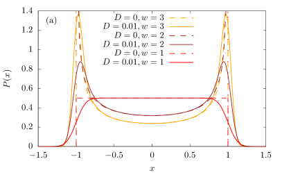
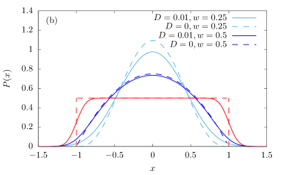
where the sum has contributions only from even $n$ (see Eqs. (21) and (22wa)). The stationary distribution then reads

$$\lim_{t\to\infty}{P(x,t)}=\sqrt{\frac{k}{{2\pi}D}}\mathchoice{e^{-\frac{kx^{2}}{2D}}}{\operatorname{exp}\!\left(-\frac{kx^{2}}{2D}\right)}{\operatorname{exp}\!\left(-\frac{kx^{2}}{2D}\right)}{\operatorname{exp}\!\left(-\frac{kx^{2}}{2D}\right)}\left(1+\sum_{\begin{subarray}{c}n=2\\ n\text{ even}\end{subarray}}^{\infty}\left(\frac{w}{\sqrt{kD}}\right)^{n}H_{n}\left(\sqrt{\frac{k}{D}}x\right)\prod_{j=1}^{n}\frac{1}{j+p_{j}/k}\right)\,,$$ (22bm)

where $p_{j}=\alpha$ if $j$ odd and $p_{j}=r\to 0$ otherwise, see figure 3 and figure 6 .

Figure 6: Stationary distribution $P(x)$ of an RnT particle in a harmonic potential for a range of values of $w$, $k$ and $D$ according to (22bm) for $D>0$ and (22bn) for $D=0$. To ease comparison, we let $\alpha=2$ and $w=\xi k$ so that the limits of the space explored by the confined particle in the diffusionless case are $\xi=\pm 1$. In (a), where $k\geq\alpha/2$, the active behaviour of the particle is manifested by the pronounced presence of the particle around $\xi$ for increasing velocity $w$. In (b), where $k\leq\alpha/2$, the self-propulsion of the particle is less prominent and its behaviour resembles that of a passive particle as the velocity $w$ decreases. In fact, for $w=0$, the particle is simply a diffusive particle confined in a harmonic potential, which is the Ornstein-Uhlenbeck process [55]. We used multiple-precision floating-point arithmetic [45] to implement Hermite polynomials up to $H_{10^{4}}\left(x\right)$ based on the GNU Scientific Library implementation [46], which are needed when the perturbative prefactor $w/\sqrt{kD}$ in Equation (22bm) is large.

Similarly, the stationary distribution of a right-moving particle is

$$\lim_{t\to\infty}P_{\phi}(x,t)\hat{=}\lim_{t\to\infty}\frac{1}{2}\Big{(}\leavevmode\hbox to43.68pt{\vbox to6.09pt{\pgfpicture\makeatletter\hbox{\hskip 21.83957pt\lower-3.04544pt\hbox to0.0pt{\pgfsys@beginscope\pgfsys@invoke{ }\definecolor{pgfstrokecolor}{rgb}{0,0,0}\pgfsys@color@rgb@stroke{0}{0}{0}\pgfsys@invoke{ }\pgfsys@color@rgb@fill{0}{0}{0}\pgfsys@invoke{ }\pgfsys@setlinewidth{0.4pt}\pgfsys@invoke{ }\nullfont\pgfsys@beginscope\pgfsys@invoke{ }\pgfsys@invoke{\lxSVG@closescope }\pgfsys@endscope\hbox to0.0pt{\pgfsys@beginscope\pgfsys@invoke{ }{ {}{{}}{} {}{}\pgfsys@beginscope\pgfsys@invoke{ }\pgfsys@setlinewidth{1.0pt}\pgfsys@invoke{ }\definecolor[named]{pgfstrokecolor}{rgb}{0,0,0}\pgfsys@color@gray@stroke{0}\pgfsys@invoke{ }{}\pgfsys@moveto{21.33957pt}{0.0pt}\pgfsys@lineto{-21.33957pt}{0.0pt}\pgfsys@stroke\pgfsys@invoke{ } \pgfsys@invoke{\lxSVG@closescope }\pgfsys@endscope{}{{}}{}{{{}}{}{}{}{}{}{}{}{}}\pgfsys@beginscope\pgfsys@invoke{ }\color[rgb]{0,0,0}\definecolor[named]{pgfstrokecolor}{rgb}{0,0,0}\pgfsys@color@gray@stroke{0}\pgfsys@invoke{ }\pgfsys@color@gray@fill{0}\pgfsys@invoke{ }\definecolor[named]{pgffillcolor}{rgb}{0,0,0}\definecolor[named]{pgffillcolor}{rgb}{0,0,0}\pgfsys@color@gray@fill{0}\pgfsys@invoke{ }{}\pgfsys@moveto{0.0pt}{0.0pt}\pgfsys@moveto{2.84544pt}{0.0pt}\pgfsys@curveto{2.84544pt}{1.5715pt}{1.5715pt}{2.84544pt}{0.0pt}{2.84544pt}\pgfsys@curveto{-1.5715pt}{2.84544pt}{-2.84544pt}{1.5715pt}{-2.84544pt}{0.0pt}\pgfsys@curveto{-2.84544pt}{-1.5715pt}{-1.5715pt}{-2.84544pt}{0.0pt}{-2.84544pt}\pgfsys@curveto{1.5715pt}{-2.84544pt}{2.84544pt}{-1.5715pt}{2.84544pt}{0.0pt}\pgfsys@closepath\pgfsys@moveto{0.0pt}{0.0pt}\pgfsys@fillstroke\pgfsys@invoke{ } \pgfsys@invoke{\lxSVG@closescope }\pgfsys@endscope} \pgfsys@invoke{\lxSVG@closescope }\pgfsys@endscope{}{}{}\hss}\pgfsys@discardpath\pgfsys@invoke{\lxSVG@closescope }\pgfsys@endscope\hss}}\lxSVG@closescope\endpgfpicture}}+\leavevmode\hbox to43.68pt{\vbox to6.09pt{\pgfpicture\makeatletter\hbox{\hskip 21.83957pt\lower-3.04544pt\hbox to0.0pt{\pgfsys@beginscope\pgfsys@invoke{ }\definecolor{pgfstrokecolor}{rgb}{0,0,0}\pgfsys@color@rgb@stroke{0}{0}{0}\pgfsys@invoke{ }\pgfsys@color@rgb@fill{0}{0}{0}\pgfsys@invoke{ }\pgfsys@setlinewidth{0.4pt}\pgfsys@invoke{ }\nullfont\pgfsys@beginscope\pgfsys@invoke{ }\pgfsys@invoke{\lxSVG@closescope }\pgfsys@endscope\hbox to0.0pt{\pgfsys@beginscope\pgfsys@invoke{ }{ {}{{}}{} {}{} {}{{}{}}{}{}{}{{}}{{}}{{}{}}{{}{}}{{{{}{}{{}} }}{{}} {}{}{} }{{{{}{}{{}} }}{{}} {{}{}{}{}} {{}{}{}{}} }{{{{}{}{{}} }}{{}} {{}{}{}{}} {{}{}{}{}} }{{{{}{}{{}} }}{{}} {{}{}{}{}} {{}{}{}{}} }{{{{}{}{{}} }}{{}} {{}{}{}{}} {{}{}{}{}} }{{{{}{}{{}} }}{{}} {{}{}{}{}} {{}{}{}{}} }{{{{}{}{{}} }}{{}} {{}{}{}{}} {{}{}{}{}} }{{{{}{}{{}} }}{{}} {{}{}{}{}} {{}{}{}{}} }{{{{}{}{{}} }}{{}} {{}{}{}{}} {{}{}{}{}} }{{{{}{}{{}} }}{{}} {{}{}{}{}} {{}{}{}{}} }{{{{}{}{{}} }}{{}} {{}{}{}{}} {{}{}{}{}} }{{{{}{}{{}} }}{{}} {{}{}{}{}} {{}{}{}{}} }{{{{}{}{{}} }}{{}} {{}{}{}{}} {{}{}{}{}} }{{{{}{}{{}} }}{{}} {{}{}{}{}} {{}{}{}{}} }{{{{}{}{{}} }}{{}} {{}{}{}{}} {{}{}{}{}} }{{{{}{}{{}} }}{{}} {{}{}{}{}} {{}{}{}{}} }{{{{}{}{{}} }}{{}} {{}} } \pgfsys@beginscope\pgfsys@invoke{ }\pgfsys@setlinewidth{1.0pt}\pgfsys@invoke{ }\definecolor[named]{pgfstrokecolor}{rgb}{0,0,0}\pgfsys@color@gray@stroke{0}\pgfsys@invoke{ }{}\pgfsys@moveto{21.33957pt}{0.0pt}\pgfsys@curveto{20.71457pt}{0.0pt}{20.40207pt}{-1.42264pt}{19.77707pt}{-1.42264pt}\pgfsys@curveto{19.32457pt}{-1.42264pt}{18.93459pt}{-0.7284pt}{18.52707pt}{0.0pt}\pgfsys@curveto{18.11957pt}{0.72838pt}{17.72957pt}{1.42264pt}{17.27707pt}{1.42264pt}\pgfsys@curveto{16.82457pt}{1.42264pt}{16.43459pt}{0.7284pt}{16.02707pt}{0.0pt}\pgfsys@curveto{15.61957pt}{-0.72838pt}{15.22957pt}{-1.42264pt}{14.77707pt}{-1.42264pt}\pgfsys@curveto{14.32457pt}{-1.42264pt}{13.93459pt}{-0.7284pt}{13.52707pt}{0.0pt}\pgfsys@curveto{13.11957pt}{0.72838pt}{12.72957pt}{1.42264pt}{12.27707pt}{1.42264pt}\pgfsys@curveto{11.82457pt}{1.42264pt}{11.43459pt}{0.7284pt}{11.02707pt}{0.0pt}\pgfsys@curveto{10.61957pt}{-0.72838pt}{10.22957pt}{-1.42264pt}{9.77707pt}{-1.42264pt}\pgfsys@curveto{9.32457pt}{-1.42264pt}{8.93459pt}{-0.7284pt}{8.52707pt}{0.0pt}\pgfsys@curveto{8.11957pt}{0.72838pt}{7.72957pt}{1.42264pt}{7.27707pt}{1.42264pt}\pgfsys@curveto{6.82457pt}{1.42264pt}{6.43459pt}{0.7284pt}{6.02707pt}{0.0pt}\pgfsys@curveto{5.61957pt}{-0.72838pt}{5.22957pt}{-1.42264pt}{4.77707pt}{-1.42264pt}\pgfsys@curveto{4.32457pt}{-1.42264pt}{3.93459pt}{-0.7284pt}{3.52707pt}{0.0pt}\pgfsys@curveto{3.11957pt}{0.72838pt}{2.72957pt}{1.42264pt}{2.27707pt}{1.42264pt}\pgfsys@curveto{1.82457pt}{1.42264pt}{1.43459pt}{0.7284pt}{1.02707pt}{0.0pt}\pgfsys@curveto{0.61957pt}{-0.72838pt}{0.22957pt}{-1.42264pt}{-0.22293pt}{-1.42264pt}\pgfsys@curveto{-0.67543pt}{-1.42264pt}{-1.06541pt}{-0.7284pt}{-1.47293pt}{0.0pt}\pgfsys@curveto{-1.88043pt}{0.72838pt}{-2.27043pt}{1.42264pt}{-2.72293pt}{1.42264pt}\pgfsys@curveto{-3.17543pt}{1.42264pt}{-3.56541pt}{0.7284pt}{-3.97293pt}{0.0pt}\pgfsys@curveto{-4.38043pt}{-0.72838pt}{-4.77043pt}{-1.42264pt}{-5.22293pt}{-1.42264pt}\pgfsys@curveto{-5.67543pt}{-1.42264pt}{-6.06541pt}{-0.7284pt}{-6.47293pt}{0.0pt}\pgfsys@curveto{-6.88043pt}{0.72838pt}{-7.27043pt}{1.42264pt}{-7.72293pt}{1.42264pt}\pgfsys@curveto{-8.17543pt}{1.42264pt}{-8.56541pt}{0.7284pt}{-8.97293pt}{0.0pt}\pgfsys@curveto{-9.38043pt}{-0.72838pt}{-9.77043pt}{-1.42264pt}{-10.22293pt}{-1.42264pt}\pgfsys@curveto{-10.67543pt}{-1.42264pt}{-11.06541pt}{-0.7284pt}{-11.47293pt}{0.0pt}\pgfsys@curveto{-11.88043pt}{0.72838pt}{-12.27043pt}{1.42264pt}{-12.72293pt}{1.42264pt}\pgfsys@curveto{-13.17543pt}{1.42264pt}{-13.56541pt}{0.7284pt}{-13.97293pt}{0.0pt}\pgfsys@curveto{-14.38043pt}{-0.72838pt}{-14.77043pt}{-1.42264pt}{-15.22293pt}{-1.42264pt}\pgfsys@curveto{-15.67543pt}{-1.42264pt}{-16.06541pt}{-0.7284pt}{-16.47293pt}{0.0pt}\pgfsys@curveto{-16.88043pt}{0.72838pt}{-17.27043pt}{1.42264pt}{-17.72293pt}{1.42264pt}\pgfsys@lineto{-21.33957pt}{0.0pt}\pgfsys@stroke\pgfsys@invoke{ } \pgfsys@invoke{\lxSVG@closescope }\pgfsys@endscope{}{{}}{}{{{}}{}{}{}{}{}{}{}{}}\pgfsys@beginscope\pgfsys@invoke{ }\color[rgb]{0,0,0}\definecolor[named]{pgfstrokecolor}{rgb}{0,0,0}\pgfsys@color@gray@stroke{0}\pgfsys@invoke{ }\pgfsys@color@gray@fill{0}\pgfsys@invoke{ }\definecolor[named]{pgffillcolor}{rgb}{0,0,0}\definecolor[named]{pgffillcolor}{rgb}{0,0,0}\pgfsys@color@gray@fill{0}\pgfsys@invoke{ }{}\pgfsys@moveto{0.0pt}{0.0pt}\pgfsys@moveto{2.84544pt}{0.0pt}\pgfsys@curveto{2.84544pt}{1.5715pt}{1.5715pt}{2.84544pt}{0.0pt}{2.84544pt}\pgfsys@curveto{-1.5715pt}{2.84544pt}{-2.84544pt}{1.5715pt}{-2.84544pt}{0.0pt}\pgfsys@curveto{-2.84544pt}{-1.5715pt}{-1.5715pt}{-2.84544pt}{0.0pt}{-2.84544pt}\pgfsys@curveto{1.5715pt}{-2.84544pt}{2.84544pt}{-1.5715pt}{2.84544pt}{0.0pt}\pgfsys@closepath\pgfsys@moveto{0.0pt}{0.0pt}\pgfsys@fillstroke\pgfsys@invoke{ } \pgfsys@invoke{\lxSVG@closescope }\pgfsys@endscope} \pgfsys@invoke{\lxSVG@closescope }\pgfsys@endscope{}{}{}\hss}\pgfsys@discardpath\pgfsys@invoke{\lxSVG@closescope }\pgfsys@endscope\hss}}\lxSVG@closescope\endpgfpicture}}+\leavevmode\hbox to43.68pt{\vbox to6.09pt{\pgfpicture\makeatletter\hbox{\hskip 21.83957pt\lower-3.04544pt\hbox to0.0pt{\pgfsys@beginscope\pgfsys@invoke{ }\definecolor{pgfstrokecolor}{rgb}{0,0,0}\pgfsys@color@rgb@stroke{0}{0}{0}\pgfsys@invoke{ }\pgfsys@color@rgb@fill{0}{0}{0}\pgfsys@invoke{ }\pgfsys@setlinewidth{0.4pt}\pgfsys@invoke{ }\nullfont\pgfsys@beginscope\pgfsys@invoke{ }\pgfsys@invoke{\lxSVG@closescope }\pgfsys@endscope\hbox to0.0pt{\pgfsys@beginscope\pgfsys@invoke{ }{ {}{{}}{} {}{}\pgfsys@beginscope\pgfsys@invoke{ }\pgfsys@setlinewidth{1.0pt}\pgfsys@invoke{ }\definecolor[named]{pgfstrokecolor}{rgb}{0,0,0}\pgfsys@color@gray@stroke{0}\pgfsys@invoke{ }{}\pgfsys@moveto{0.0pt}{0.0pt}\pgfsys@lineto{-21.33957pt}{0.0pt}\pgfsys@stroke\pgfsys@invoke{ } \pgfsys@invoke{\lxSVG@closescope }\pgfsys@endscope{}{{}}{} {}{} {}{{}{}}{}{}{}{{}}{{}}{{}{}}{{}{}}{{{{}{}{{}} }}{{}} {}{}{} }{{{{}{}{{}} }}{{}} {}{}{} }{{{{}{}{{}} }}{{}} {{}} } \pgfsys@beginscope\pgfsys@invoke{ }\pgfsys@setlinewidth{1.0pt}\pgfsys@invoke{ }\definecolor[named]{pgfstrokecolor}{rgb}{0,0,0}\pgfsys@color@gray@stroke{0}\pgfsys@invoke{ }{}\pgfsys@moveto{21.33957pt}{0.0pt}\pgfsys@curveto{20.71457pt}{0.0pt}{20.40207pt}{-1.42264pt}{19.77707pt}{-1.42264pt}\pgfsys@curveto{19.15207pt}{-1.42264pt}{18.83957pt}{0.0pt}{18.21457pt}{0.0pt}\pgfsys@lineto{0.0pt}{0.0pt}\pgfsys@stroke\pgfsys@invoke{ } \pgfsys@invoke{\lxSVG@closescope }\pgfsys@endscope{}{{}}{}{{{}}{}{}{}{}{}{}{}{}}\pgfsys@beginscope\pgfsys@invoke{ }\color[rgb]{0,0,0}\definecolor[named]{pgfstrokecolor}{rgb}{0,0,0}\pgfsys@color@gray@stroke{0}\pgfsys@invoke{ }\pgfsys@color@gray@fill{0}\pgfsys@invoke{ }\definecolor[named]{pgffillcolor}{rgb}{0,0,0}\definecolor[named]{pgffillcolor}{rgb}{0,0,0}\pgfsys@color@gray@fill{0}\pgfsys@invoke{ }{}\pgfsys@moveto{0.0pt}{0.0pt}\pgfsys@moveto{2.84544pt}{0.0pt}\pgfsys@curveto{2.84544pt}{1.5715pt}{1.5715pt}{2.84544pt}{0.0pt}{2.84544pt}\pgfsys@curveto{-1.5715pt}{2.84544pt}{-2.84544pt}{1.5715pt}{-2.84544pt}{0.0pt}\pgfsys@curveto{-2.84544pt}{-1.5715pt}{-1.5715pt}{-2.84544pt}{0.0pt}{-2.84544pt}\pgfsys@curveto{1.5715pt}{-2.84544pt}{2.84544pt}{-1.5715pt}{2.84544pt}{0.0pt}\pgfsys@closepath\pgfsys@moveto{0.0pt}{0.0pt}\pgfsys@fillstroke\pgfsys@invoke{ } \pgfsys@invoke{\lxSVG@closescope }\pgfsys@endscope} \pgfsys@invoke{\lxSVG@closescope }\pgfsys@endscope{}{}{}\hss}\pgfsys@discardpath\pgfsys@invoke{\lxSVG@closescope }\pgfsys@endscope\hss}}\lxSVG@closescope\endpgfpicture}}+\leavevmode\hbox to43.68pt{\vbox to6.09pt{\pgfpicture\makeatletter\hbox{\hskip 21.83957pt\lower-3.04544pt\hbox to0.0pt{\pgfsys@beginscope\pgfsys@invoke{ }\definecolor{pgfstrokecolor}{rgb}{0,0,0}\pgfsys@color@rgb@stroke{0}{0}{0}\pgfsys@invoke{ }\pgfsys@color@rgb@fill{0}{0}{0}\pgfsys@invoke{ }\pgfsys@setlinewidth{0.4pt}\pgfsys@invoke{ }\nullfont\pgfsys@beginscope\pgfsys@invoke{ }\pgfsys@invoke{\lxSVG@closescope }\pgfsys@endscope\hbox to0.0pt{\pgfsys@beginscope\pgfsys@invoke{ }{ {}{{}}{} {}{}\pgfsys@beginscope\pgfsys@invoke{ }\pgfsys@setlinewidth{1.0pt}\pgfsys@invoke{ }\definecolor[named]{pgfstrokecolor}{rgb}{0,0,0}\pgfsys@color@gray@stroke{0}\pgfsys@invoke{ }{}\pgfsys@moveto{21.33957pt}{0.0pt}\pgfsys@lineto{0.0pt}{0.0pt}\pgfsys@stroke\pgfsys@invoke{ } \pgfsys@invoke{\lxSVG@closescope }\pgfsys@endscope{}{{}}{} {}{} {}{{}{}}{}{}{}{{}}{{}}{{}{}}{{}{}}{{{{}{}{{}} }}{{}} {}{}{} }{{{{}{}{{}} }}{{}} {{}{}{}{}} {{}{}{}{}} }{{{{}{}{{}} }}{{}} {{}{}{}{}} {{}{}{}{}} }{{{{}{}{{}} }}{{}} {{}{}{}{}} {{}{}{}{}} }{{{{}{}{{}} }}{{}} {{}{}{}{}} {{}{}{}{}} }{{{{}{}{{}} }}{{}} {{}{}{}{}} {{}{}{}{}} }{{{{}{}{{}} }}{{}} {{}{}{}{}} {{}{}{}{}} }{{{{}{}{{}} }}{{}} {{}{}{}{}} {{}{}{}{}} }{{{{}{}{{}} }}{{}} {{}} } \pgfsys@beginscope\pgfsys@invoke{ }\pgfsys@setlinewidth{1.0pt}\pgfsys@invoke{ }\definecolor[named]{pgfstrokecolor}{rgb}{0,0,0}\pgfsys@color@gray@stroke{0}\pgfsys@invoke{ }{}\pgfsys@moveto{0.0pt}{0.0pt}\pgfsys@curveto{-0.625pt}{0.0pt}{-0.9375pt}{-1.42264pt}{-1.5625pt}{-1.42264pt}\pgfsys@curveto{-2.015pt}{-1.42264pt}{-2.40498pt}{-0.7284pt}{-2.8125pt}{0.0pt}\pgfsys@curveto{-3.22pt}{0.72838pt}{-3.61pt}{1.42264pt}{-4.0625pt}{1.42264pt}\pgfsys@curveto{-4.515pt}{1.42264pt}{-4.90498pt}{0.7284pt}{-5.3125pt}{0.0pt}\pgfsys@curveto{-5.72pt}{-0.72838pt}{-6.11pt}{-1.42264pt}{-6.5625pt}{-1.42264pt}\pgfsys@curveto{-7.015pt}{-1.42264pt}{-7.40498pt}{-0.7284pt}{-7.8125pt}{0.0pt}\pgfsys@curveto{-8.22pt}{0.72838pt}{-8.61pt}{1.42264pt}{-9.0625pt}{1.42264pt}\pgfsys@curveto{-9.515pt}{1.42264pt}{-9.90498pt}{0.7284pt}{-10.3125pt}{0.0pt}\pgfsys@curveto{-10.72pt}{-0.72838pt}{-11.11pt}{-1.42264pt}{-11.5625pt}{-1.42264pt}\pgfsys@curveto{-12.015pt}{-1.42264pt}{-12.40498pt}{-0.7284pt}{-12.8125pt}{0.0pt}\pgfsys@curveto{-13.22pt}{0.72838pt}{-13.61pt}{1.42264pt}{-14.0625pt}{1.42264pt}\pgfsys@curveto{-14.515pt}{1.42264pt}{-14.90498pt}{0.7284pt}{-15.3125pt}{0.0pt}\pgfsys@curveto{-15.72pt}{-0.72838pt}{-16.11pt}{-1.42264pt}{-16.5625pt}{-1.42264pt}\pgfsys@curveto{-17.015pt}{-1.42264pt}{-17.40498pt}{-0.7284pt}{-17.8125pt}{0.0pt}\pgfsys@curveto{-18.22pt}{0.72838pt}{-18.61pt}{1.42264pt}{-19.0625pt}{1.42264pt}\pgfsys@lineto{-21.33957pt}{0.0pt}\pgfsys@stroke\pgfsys@invoke{ } \pgfsys@invoke{\lxSVG@closescope }\pgfsys@endscope{}{{}}{}{{{}}{}{}{}{}{}{}{}{}}\pgfsys@beginscope\pgfsys@invoke{ }\color[rgb]{0,0,0}\definecolor[named]{pgfstrokecolor}{rgb}{0,0,0}\pgfsys@color@gray@stroke{0}\pgfsys@invoke{ }\pgfsys@color@gray@fill{0}\pgfsys@invoke{ }\definecolor[named]{pgffillcolor}{rgb}{0,0,0}\definecolor[named]{pgffillcolor}{rgb}{0,0,0}\pgfsys@color@gray@fill{0}\pgfsys@invoke{ }{}\pgfsys@moveto{0.0pt}{0.0pt}\pgfsys@moveto{2.84544pt}{0.0pt}\pgfsys@curveto{2.84544pt}{1.5715pt}{1.5715pt}{2.84544pt}{0.0pt}{2.84544pt}\pgfsys@curveto{-1.5715pt}{2.84544pt}{-2.84544pt}{1.5715pt}{-2.84544pt}{0.0pt}\pgfsys@curveto{-2.84544pt}{-1.5715pt}{-1.5715pt}{-2.84544pt}{0.0pt}{-2.84544pt}\pgfsys@curveto{1.5715pt}{-2.84544pt}{2.84544pt}{-1.5715pt}{2.84544pt}{0.0pt}\pgfsys@closepath\pgfsys@moveto{0.0pt}{0.0pt}\pgfsys@fillstroke\pgfsys@invoke{ } \pgfsys@invoke{\lxSVG@closescope }\pgfsys@endscope} \pgfsys@invoke{\lxSVG@closescope }\pgfsys@endscope{}{}{}\hss}\pgfsys@discardpath\pgfsys@invoke{\lxSVG@closescope }\pgfsys@endscope\hss}}\lxSVG@closescope\endpgfpicture}}\Big{)}$$

$$=\lim_{t\to\infty}\frac{1}{2}\Big{(}\leavevmode\hbox to43.68pt{\vbox to6.09pt{\pgfpicture\makeatletter\hbox{\hskip 21.83957pt\lower-3.04544pt\hbox to0.0pt{\pgfsys@beginscope\pgfsys@invoke{ }\definecolor{pgfstrokecolor}{rgb}{0,0,0}\pgfsys@color@rgb@stroke{0}{0}{0}\pgfsys@invoke{ }\pgfsys@color@rgb@fill{0}{0}{0}\pgfsys@invoke{ }\pgfsys@setlinewidth{0.4pt}\pgfsys@invoke{ }\nullfont\pgfsys@beginscope\pgfsys@invoke{ }\pgfsys@invoke{\lxSVG@closescope }\pgfsys@endscope\hbox to0.0pt{\pgfsys@beginscope\pgfsys@invoke{ }{ {}{{}}{} {}{}\pgfsys@beginscope\pgfsys@invoke{ }\pgfsys@setlinewidth{1.0pt}\pgfsys@invoke{ }\definecolor[named]{pgfstrokecolor}{rgb}{0,0,0}\pgfsys@color@gray@stroke{0}\pgfsys@invoke{ }{}\pgfsys@moveto{21.33957pt}{0.0pt}\pgfsys@lineto{-21.33957pt}{0.0pt}\pgfsys@stroke\pgfsys@invoke{ } \pgfsys@invoke{\lxSVG@closescope }\pgfsys@endscope{}{{}}{}{{{}}{}{}{}{}{}{}{}{}}\pgfsys@beginscope\pgfsys@invoke{ }\color[rgb]{0,0,0}\definecolor[named]{pgfstrokecolor}{rgb}{0,0,0}\pgfsys@color@gray@stroke{0}\pgfsys@invoke{ }\pgfsys@color@gray@fill{0}\pgfsys@invoke{ }\definecolor[named]{pgffillcolor}{rgb}{0,0,0}\definecolor[named]{pgffillcolor}{rgb}{0,0,0}\pgfsys@color@gray@fill{0}\pgfsys@invoke{ }{}\pgfsys@moveto{0.0pt}{0.0pt}\pgfsys@moveto{2.84544pt}{0.0pt}\pgfsys@curveto{2.84544pt}{1.5715pt}{1.5715pt}{2.84544pt}{0.0pt}{2.84544pt}\pgfsys@curveto{-1.5715pt}{2.84544pt}{-2.84544pt}{1.5715pt}{-2.84544pt}{0.0pt}\pgfsys@curveto{-2.84544pt}{-1.5715pt}{-1.5715pt}{-2.84544pt}{0.0pt}{-2.84544pt}\pgfsys@curveto{1.5715pt}{-2.84544pt}{2.84544pt}{-1.5715pt}{2.84544pt}{0.0pt}\pgfsys@closepath\pgfsys@moveto{0.0pt}{0.0pt}\pgfsys@fillstroke\pgfsys@invoke{ } \pgfsys@invoke{\lxSVG@closescope }\pgfsys@endscope} \pgfsys@invoke{\lxSVG@closescope }\pgfsys@endscope{}{}{}\hss}\pgfsys@discardpath\pgfsys@invoke{\lxSVG@closescope }\pgfsys@endscope\hss}}\lxSVG@closescope\endpgfpicture}}+\leavevmode\hbox to43.68pt{\vbox to6.09pt{\pgfpicture\makeatletter\hbox{\hskip 21.83957pt\lower-3.04544pt\hbox to0.0pt{\pgfsys@beginscope\pgfsys@invoke{ }\definecolor{pgfstrokecolor}{rgb}{0,0,0}\pgfsys@color@rgb@stroke{0}{0}{0}\pgfsys@invoke{ }\pgfsys@color@rgb@fill{0}{0}{0}\pgfsys@invoke{ }\pgfsys@setlinewidth{0.4pt}\pgfsys@invoke{ }\nullfont\pgfsys@beginscope\pgfsys@invoke{ }\pgfsys@invoke{\lxSVG@closescope }\pgfsys@endscope\hbox to0.0pt{\pgfsys@beginscope\pgfsys@invoke{ }{ {}{{}}{} {}{}\pgfsys@beginscope\pgfsys@invoke{ }\pgfsys@setlinewidth{1.0pt}\pgfsys@invoke{ }\definecolor[named]{pgfstrokecolor}{rgb}{0,0,0}\pgfsys@color@gray@stroke{0}\pgfsys@invoke{ }{}\pgfsys@moveto{21.33957pt}{0.0pt}\pgfsys@lineto{0.0pt}{0.0pt}\pgfsys@stroke\pgfsys@invoke{ } \pgfsys@invoke{\lxSVG@closescope }\pgfsys@endscope{}{{}}{} {}{} {}{{}{}}{}{}{}{{}}{{}}{{}{}}{{}{}}{{{{}{}{{}} }}{{}} {}{}{} }{{{{}{}{{}} }}{{}} {{}{}{}{}} {{}{}{}{}} }{{{{}{}{{}} }}{{}} {{}{}{}{}} {{}{}{}{}} }{{{{}{}{{}} }}{{}} {{}{}{}{}} {{}{}{}{}} }{{{{}{}{{}} }}{{}} {{}{}{}{}} {{}{}{}{}} }{{{{}{}{{}} }}{{}} {{}{}{}{}} {{}{}{}{}} }{{{{}{}{{}} }}{{}} {{}{}{}{}} {{}{}{}{}} }{{{{}{}{{}} }}{{}} {{}{}{}{}} {{}{}{}{}} }{{{{}{}{{}} }}{{}} {{}} } \pgfsys@beginscope\pgfsys@invoke{ }\pgfsys@setlinewidth{1.0pt}\pgfsys@invoke{ }\definecolor[named]{pgfstrokecolor}{rgb}{0,0,0}\pgfsys@color@gray@stroke{0}\pgfsys@invoke{ }{}\pgfsys@moveto{0.0pt}{0.0pt}\pgfsys@curveto{-0.625pt}{0.0pt}{-0.9375pt}{-1.42264pt}{-1.5625pt}{-1.42264pt}\pgfsys@curveto{-2.015pt}{-1.42264pt}{-2.40498pt}{-0.7284pt}{-2.8125pt}{0.0pt}\pgfsys@curveto{-3.22pt}{0.72838pt}{-3.61pt}{1.42264pt}{-4.0625pt}{1.42264pt}\pgfsys@curveto{-4.515pt}{1.42264pt}{-4.90498pt}{0.7284pt}{-5.3125pt}{0.0pt}\pgfsys@curveto{-5.72pt}{-0.72838pt}{-6.11pt}{-1.42264pt}{-6.5625pt}{-1.42264pt}\pgfsys@curveto{-7.015pt}{-1.42264pt}{-7.40498pt}{-0.7284pt}{-7.8125pt}{0.0pt}\pgfsys@curveto{-8.22pt}{0.72838pt}{-8.61pt}{1.42264pt}{-9.0625pt}{1.42264pt}\pgfsys@curveto{-9.515pt}{1.42264pt}{-9.90498pt}{0.7284pt}{-10.3125pt}{0.0pt}\pgfsys@curveto{-10.72pt}{-0.72838pt}{-11.11pt}{-1.42264pt}{-11.5625pt}{-1.42264pt}\pgfsys@curveto{-12.015pt}{-1.42264pt}{-12.40498pt}{-0.7284pt}{-12.8125pt}{0.0pt}\pgfsys@curveto{-13.22pt}{0.72838pt}{-13.61pt}{1.42264pt}{-14.0625pt}{1.42264pt}\pgfsys@curveto{-14.515pt}{1.42264pt}{-14.90498pt}{0.7284pt}{-15.3125pt}{0.0pt}\pgfsys@curveto{-15.72pt}{-0.72838pt}{-16.11pt}{-1.42264pt}{-16.5625pt}{-1.42264pt}\pgfsys@curveto{-17.015pt}{-1.42264pt}{-17.40498pt}{-0.7284pt}{-17.8125pt}{0.0pt}\pgfsys@curveto{-18.22pt}{0.72838pt}{-18.61pt}{1.42264pt}{-19.0625pt}{1.42264pt}\pgfsys@lineto{-21.33957pt}{0.0pt}\pgfsys@stroke\pgfsys@invoke{ } \pgfsys@invoke{\lxSVG@closescope }\pgfsys@endscope{}{{}}{}{{{}}{}{}{}{}{}{}{}{}}\pgfsys@beginscope\pgfsys@invoke{ }\color[rgb]{0,0,0}\definecolor[named]{pgfstrokecolor}{rgb}{0,0,0}\pgfsys@color@gray@stroke{0}\pgfsys@invoke{ }\pgfsys@color@gray@fill{0}\pgfsys@invoke{ }\definecolor[named]{pgffillcolor}{rgb}{0,0,0}\definecolor[named]{pgffillcolor}{rgb}{0,0,0}\pgfsys@color@gray@fill{0}\pgfsys@invoke{ }{}\pgfsys@moveto{0.0pt}{0.0pt}\pgfsys@moveto{2.84544pt}{0.0pt}\pgfsys@curveto{2.84544pt}{1.5715pt}{1.5715pt}{2.84544pt}{0.0pt}{2.84544pt}\pgfsys@curveto{-1.5715pt}{2.84544pt}{-2.84544pt}{1.5715pt}{-2.84544pt}{0.0pt}\pgfsys@curveto{-2.84544pt}{-1.5715pt}{-1.5715pt}{-2.84544pt}{0.0pt}{-2.84544pt}\pgfsys@curveto{1.5715pt}{-2.84544pt}{2.84544pt}{-1.5715pt}{2.84544pt}{0.0pt}\pgfsys@closepath\pgfsys@moveto{0.0pt}{0.0pt}\pgfsys@fillstroke\pgfsys@invoke{ } \pgfsys@invoke{\lxSVG@closescope }\pgfsys@endscope} \pgfsys@invoke{\lxSVG@closescope }\pgfsys@endscope{}{}{}\hss}\pgfsys@discardpath\pgfsys@invoke{\lxSVG@closescope }\pgfsys@endscope\hss}}\lxSVG@closescope\endpgfpicture}}\Big{)}\,,$$ (22bo)

whose contribution $\lim_{t\to\infty}\leavevmode\hbox to22.34pt{\vbox to3.25pt{\pgfpicture\makeatletter\hbox{\hskip 11.16978pt\lower-1.62271pt\hbox to0.0pt{\pgfsys@beginscope\pgfsys@invoke{ }\definecolor{pgfstrokecolor}{rgb}{0,0,0}\pgfsys@color@rgb@stroke{0}{0}{0}\pgfsys@invoke{ }\pgfsys@color@rgb@fill{0}{0}{0}\pgfsys@invoke{ }\pgfsys@setlinewidth{0.4pt}\pgfsys@invoke{ }\nullfont\pgfsys@beginscope\pgfsys@invoke{ }\pgfsys@invoke{\lxSVG@closescope }\pgfsys@endscope\hbox to0.0pt{\pgfsys@beginscope\pgfsys@invoke{ }{{}}{ {}{{}}{} {}{}\pgfsys@beginscope\pgfsys@invoke{ }\pgfsys@setlinewidth{1.0pt}\pgfsys@invoke{ }\definecolor[named]{pgfstrokecolor}{rgb}{0,0,0}\pgfsys@color@gray@stroke{0}\pgfsys@invoke{ }{}\pgfsys@moveto{10.66978pt}{0.0pt}\pgfsys@lineto{-10.66978pt}{0.0pt}\pgfsys@stroke\pgfsys@invoke{ } \pgfsys@invoke{\lxSVG@closescope }\pgfsys@endscope{}{{}}{}{{{}}{}{}{}{}{}{}{}{}}\pgfsys@beginscope\pgfsys@invoke{ }\color[rgb]{0,0,0}\definecolor[named]{pgfstrokecolor}{rgb}{0,0,0}\pgfsys@color@gray@stroke{0}\pgfsys@invoke{ }\pgfsys@color@gray@fill{0}\pgfsys@invoke{ }\definecolor[named]{pgffillcolor}{rgb}{0,0,0}\definecolor[named]{pgffillcolor}{rgb}{0,0,0}\pgfsys@color@gray@fill{0}\pgfsys@invoke{ }{}\pgfsys@moveto{0.0pt}{0.0pt}\pgfsys@moveto{1.42271pt}{0.0pt}\pgfsys@curveto{1.42271pt}{0.78575pt}{0.78575pt}{1.42271pt}{0.0pt}{1.42271pt}\pgfsys@curveto{-0.78575pt}{1.42271pt}{-1.42271pt}{0.78575pt}{-1.42271pt}{0.0pt}\pgfsys@curveto{-1.42271pt}{-0.78575pt}{-0.78575pt}{-1.42271pt}{0.0pt}{-1.42271pt}\pgfsys@curveto{0.78575pt}{-1.42271pt}{1.42271pt}{-0.78575pt}{1.42271pt}{0.0pt}\pgfsys@closepath\pgfsys@moveto{0.0pt}{0.0pt}\pgfsys@fillstroke\pgfsys@invoke{ } \pgfsys@invoke{\lxSVG@closescope }\pgfsys@endscope} \pgfsys@invoke{\lxSVG@closescope }\pgfsys@endscope{}{}{}\hss}\pgfsys@discardpath\pgfsys@invoke{\lxSVG@closescope }\pgfsys@endscope\hss}}\lxSVG@closescope\endpgfpicture}}$ is known from (22bm). As above, only diagrams that have index $m=0$ remain in the limit $t\to\infty$, so that

$$\lim_{t\to\infty}\leavevmode\hbox to43.68pt{\vbox to6.09pt{\pgfpicture\makeatletter\hbox{\hskip 21.83957pt\lower-3.04544pt\hbox to0.0pt{\pgfsys@beginscope\pgfsys@invoke{ }\definecolor{pgfstrokecolor}{rgb}{0,0,0}\pgfsys@color@rgb@stroke{0}{0}{0}\pgfsys@invoke{ }\pgfsys@color@rgb@fill{0}{0}{0}\pgfsys@invoke{ }\pgfsys@setlinewidth{0.4pt}\pgfsys@invoke{ }\nullfont\pgfsys@beginscope\pgfsys@invoke{ }\pgfsys@invoke{\lxSVG@closescope }\pgfsys@endscope\hbox to0.0pt{\pgfsys@beginscope\pgfsys@invoke{ }{ {}{{}}{} {}{}\pgfsys@beginscope\pgfsys@invoke{ }\pgfsys@setlinewidth{1.0pt}\pgfsys@invoke{ }\definecolor[named]{pgfstrokecolor}{rgb}{0,0,0}\pgfsys@color@gray@stroke{0}\pgfsys@invoke{ }{}\pgfsys@moveto{21.33957pt}{0.0pt}\pgfsys@lineto{0.0pt}{0.0pt}\pgfsys@stroke\pgfsys@invoke{ } \pgfsys@invoke{\lxSVG@closescope }\pgfsys@endscope{}{{}}{} {}{} {}{{}{}}{}{}{}{{}}{{}}{{}{}}{{}{}}{{{{}{}{{}} }}{{}} {}{}{} }{{{{}{}{{}} }}{{}} {{}{}{}{}} {{}{}{}{}} }{{{{}{}{{}} }}{{}} {{}{}{}{}} {{}{}{}{}} }{{{{}{}{{}} }}{{}} {{}{}{}{}} {{}{}{}{}} }{{{{}{}{{}} }}{{}} {{}{}{}{}} {{}{}{}{}} }{{{{}{}{{}} }}{{}} {{}{}{}{}} {{}{}{}{}} }{{{{}{}{{}} }}{{}} {{}{}{}{}} {{}{}{}{}} }{{{{}{}{{}} }}{{}} {{}{}{}{}} {{}{}{}{}} }{{{{}{}{{}} }}{{}} {{}} } \pgfsys@beginscope\pgfsys@invoke{ }\pgfsys@setlinewidth{1.0pt}\pgfsys@invoke{ }\definecolor[named]{pgfstrokecolor}{rgb}{0,0,0}\pgfsys@color@gray@stroke{0}\pgfsys@invoke{ }{}\pgfsys@moveto{0.0pt}{0.0pt}\pgfsys@curveto{-0.625pt}{0.0pt}{-0.9375pt}{-1.42264pt}{-1.5625pt}{-1.42264pt}\pgfsys@curveto{-2.015pt}{-1.42264pt}{-2.40498pt}{-0.7284pt}{-2.8125pt}{0.0pt}\pgfsys@curveto{-3.22pt}{0.72838pt}{-3.61pt}{1.42264pt}{-4.0625pt}{1.42264pt}\pgfsys@curveto{-4.515pt}{1.42264pt}{-4.90498pt}{0.7284pt}{-5.3125pt}{0.0pt}\pgfsys@curveto{-5.72pt}{-0.72838pt}{-6.11pt}{-1.42264pt}{-6.5625pt}{-1.42264pt}\pgfsys@curveto{-7.015pt}{-1.42264pt}{-7.40498pt}{-0.7284pt}{-7.8125pt}{0.0pt}\pgfsys@curveto{-8.22pt}{0.72838pt}{-8.61pt}{1.42264pt}{-9.0625pt}{1.42264pt}\pgfsys@curveto{-9.515pt}{1.42264pt}{-9.90498pt}{0.7284pt}{-10.3125pt}{0.0pt}\pgfsys@curveto{-10.72pt}{-0.72838pt}{-11.11pt}{-1.42264pt}{-11.5625pt}{-1.42264pt}\pgfsys@curveto{-12.015pt}{-1.42264pt}{-12.40498pt}{-0.7284pt}{-12.8125pt}{0.0pt}\pgfsys@curveto{-13.22pt}{0.72838pt}{-13.61pt}{1.42264pt}{-14.0625pt}{1.42264pt}\pgfsys@curveto{-14.515pt}{1.42264pt}{-14.90498pt}{0.7284pt}{-15.3125pt}{0.0pt}\pgfsys@curveto{-15.72pt}{-0.72838pt}{-16.11pt}{-1.42264pt}{-16.5625pt}{-1.42264pt}\pgfsys@curveto{-17.015pt}{-1.42264pt}{-17.40498pt}{-0.7284pt}{-17.8125pt}{0.0pt}\pgfsys@curveto{-18.22pt}{0.72838pt}{-18.61pt}{1.42264pt}{-19.0625pt}{1.42264pt}\pgfsys@lineto{-21.33957pt}{0.0pt}\pgfsys@stroke\pgfsys@invoke{ } \pgfsys@invoke{\lxSVG@closescope }\pgfsys@endscope{}{{}}{}{{{}}{}{}{}{}{}{}{}{}}\pgfsys@beginscope\pgfsys@invoke{ }\color[rgb]{0,0,0}\definecolor[named]{pgfstrokecolor}{rgb}{0,0,0}\pgfsys@color@gray@stroke{0}\pgfsys@invoke{ }\pgfsys@color@gray@fill{0}\pgfsys@invoke{ }\definecolor[named]{pgffillcolor}{rgb}{0,0,0}\definecolor[named]{pgffillcolor}{rgb}{0,0,0}\pgfsys@color@gray@fill{0}\pgfsys@invoke{ }{}\pgfsys@moveto{0.0pt}{0.0pt}\pgfsys@moveto{2.84544pt}{0.0pt}\pgfsys@curveto{2.84544pt}{1.5715pt}{1.5715pt}{2.84544pt}{0.0pt}{2.84544pt}\pgfsys@curveto{-1.5715pt}{2.84544pt}{-2.84544pt}{1.5715pt}{-2.84544pt}{0.0pt}\pgfsys@curveto{-2.84544pt}{-1.5715pt}{-1.5715pt}{-2.84544pt}{0.0pt}{-2.84544pt}\pgfsys@curveto{1.5715pt}{-2.84544pt}{2.84544pt}{-1.5715pt}{2.84544pt}{0.0pt}\pgfsys@closepath\pgfsys@moveto{0.0pt}{0.0pt}\pgfsys@fillstroke\pgfsys@invoke{ } \pgfsys@invoke{\lxSVG@closescope }\pgfsys@endscope} \pgfsys@invoke{\lxSVG@closescope }\pgfsys@endscope{}{}{}\hss}\pgfsys@discardpath\pgfsys@invoke{\lxSVG@closescope }\pgfsys@endscope\hss}}\lxSVG@closescope\endpgfpicture}}=\lim_{t\to\infty}\frac{k}{D}\sum_{n\geq 1}\leavevmode\hbox to61.88pt{\vbox to18.31pt{\pgfpicture\makeatletter\hbox{\hskip 30.381pt\lower-3.04544pt\hbox to0.0pt{\pgfsys@beginscope\pgfsys@invoke{ }\definecolor{pgfstrokecolor}{rgb}{0,0,0}\pgfsys@color@rgb@stroke{0}{0}{0}\pgfsys@invoke{ }\pgfsys@color@rgb@fill{0}{0}{0}\pgfsys@invoke{ }\pgfsys@setlinewidth{0.4pt}\pgfsys@invoke{ }\nullfont\pgfsys@beginscope\pgfsys@invoke{ }\pgfsys@invoke{\lxSVG@closescope }\pgfsys@endscope\hbox to0.0pt{\pgfsys@beginscope\pgfsys@invoke{ }{ {}{{}}{} {}{}{}{}{{{}{}}}\pgfsys@beginscope\pgfsys@invoke{ }\pgfsys@setlinewidth{1.0pt}\pgfsys@invoke{ }\definecolor[named]{pgfstrokecolor}{rgb}{0,0,0}\pgfsys@color@gray@stroke{0}\pgfsys@invoke{ }{}\pgfsys@moveto{21.33957pt}{0.0pt}\pgfsys@lineto{0.0pt}{0.0pt}\pgfsys@stroke\pgfsys@invoke{ }\hbox{\hbox{{\pgfsys@beginscope\pgfsys@invoke{ }{{}{}{{ {}{}}}{ {}{}} {{}{{}}}{{}{}}{}{{}{}} { }{{{{}}\pgfsys@beginscope\pgfsys@invoke{ }\pgfsys@transformcm{1.0}{0.0}{0.0}{1.0}{14.51181pt}{5.77744pt}\pgfsys@invoke{ }\hbox{{\definecolor{pgfstrokecolor}{rgb}{0,0,0}\pgfsys@color@rgb@stroke{0}{0}{0}\pgfsys@invoke{ }\pgfsys@color@rgb@fill{0}{0}{0}\pgfsys@invoke{ }\hbox{{${}_{0},t_{0}$}} }}\pgfsys@invoke{\lxSVG@closescope }\pgfsys@endscope}}} \pgfsys@invoke{\lxSVG@closescope }\pgfsys@endscope}}} \pgfsys@invoke{\lxSVG@closescope }\pgfsys@endscope{}{{}}{} {}{}{}{}{{{}{}}} {}{{}{}}{}{}{}{{}}{{}}{{}{}}{{}{}}{{{{}{}{{}} }}{{}} {}{}{} }{{{{}{}{{}} }}{{}} {{}{}{}{}} {{}{}{}{}} }{{{{}{}{{}} }}{{}} {{}{}{}{}} {{}{}{}{}} }{{{{}{}{{}} }}{{}} {{}{}{}{}} {{}{}{}{}} }{{{{}{}{{}} }}{{}} {{}{}{}{}} {{}{}{}{}} }{{{{}{}{{}} }}{{}} {{}{}{}{}} {{}{}{}{}} }{{{{}{}{{}} }}{{}} {{}{}{}{}} {{}{}{}{}} }{{{{}{}{{}} }}{{}} {{}{}{}{}} {{}{}{}{}} }{{{{}{}{{}} }}{{}} {{}} } \pgfsys@beginscope\pgfsys@invoke{ }\pgfsys@setlinewidth{1.0pt}\pgfsys@invoke{ }\definecolor[named]{pgfstrokecolor}{rgb}{0,0,0}\pgfsys@color@gray@stroke{0}\pgfsys@invoke{ }{}\pgfsys@moveto{0.0pt}{0.0pt}\pgfsys@curveto{-0.625pt}{0.0pt}{-0.9375pt}{-1.42264pt}{-1.5625pt}{-1.42264pt}\pgfsys@curveto{-2.015pt}{-1.42264pt}{-2.40498pt}{-0.7284pt}{-2.8125pt}{0.0pt}\pgfsys@curveto{-3.22pt}{0.72838pt}{-3.61pt}{1.42264pt}{-4.0625pt}{1.42264pt}\pgfsys@curveto{-4.515pt}{1.42264pt}{-4.90498pt}{0.7284pt}{-5.3125pt}{0.0pt}\pgfsys@curveto{-5.72pt}{-0.72838pt}{-6.11pt}{-1.42264pt}{-6.5625pt}{-1.42264pt}\pgfsys@curveto{-7.015pt}{-1.42264pt}{-7.40498pt}{-0.7284pt}{-7.8125pt}{0.0pt}\pgfsys@curveto{-8.22pt}{0.72838pt}{-8.61pt}{1.42264pt}{-9.0625pt}{1.42264pt}\pgfsys@curveto{-9.515pt}{1.42264pt}{-9.90498pt}{0.7284pt}{-10.3125pt}{0.0pt}\pgfsys@curveto{-10.72pt}{-0.72838pt}{-11.11pt}{-1.42264pt}{-11.5625pt}{-1.42264pt}\pgfsys@curveto{-12.015pt}{-1.42264pt}{-12.40498pt}{-0.7284pt}{-12.8125pt}{0.0pt}\pgfsys@curveto{-13.22pt}{0.72838pt}{-13.61pt}{1.42264pt}{-14.0625pt}{1.42264pt}\pgfsys@curveto{-14.515pt}{1.42264pt}{-14.90498pt}{0.7284pt}{-15.3125pt}{0.0pt}\pgfsys@curveto{-15.72pt}{-0.72838pt}{-16.11pt}{-1.42264pt}{-16.5625pt}{-1.42264pt}\pgfsys@curveto{-17.015pt}{-1.42264pt}{-17.40498pt}{-0.7284pt}{-17.8125pt}{0.0pt}\pgfsys@curveto{-18.22pt}{0.72838pt}{-18.61pt}{1.42264pt}{-19.0625pt}{1.42264pt}\pgfsys@lineto{-21.33957pt}{0.0pt}\pgfsys@stroke\pgfsys@invoke{ }\hbox{\hbox{{\pgfsys@beginscope\pgfsys@invoke{ }{{}{}{{ {}{}}}{ {}{}} {{}{{}}}{{}{}}{}{{}{}} { }{{{{}}\pgfsys@beginscope\pgfsys@invoke{ }\pgfsys@transformcm{1.0}{0.0}{0.0}{1.0}{-27.04799pt}{5.77744pt}\pgfsys@invoke{ }\hbox{{\definecolor{pgfstrokecolor}{rgb}{0,0,0}\pgfsys@color@rgb@stroke{0}{0}{0}\pgfsys@invoke{ }\pgfsys@color@rgb@fill{0}{0}{0}\pgfsys@invoke{ }\hbox{{${}_{n},t$}} }}\pgfsys@invoke{\lxSVG@closescope }\pgfsys@endscope}}} \pgfsys@invoke{\lxSVG@closescope }\pgfsys@endscope}}} \pgfsys@invoke{\lxSVG@closescope }\pgfsys@endscope{}{{}}{}{{{}}{}{}{}{}{}{}{}{}}\pgfsys@beginscope\pgfsys@invoke{ }\color[rgb]{0,0,0}\definecolor[named]{pgfstrokecolor}{rgb}{0,0,0}\pgfsys@color@gray@stroke{0}\pgfsys@invoke{ }\pgfsys@color@gray@fill{0}\pgfsys@invoke{ }\definecolor[named]{pgffillcolor}{rgb}{0,0,0}\definecolor[named]{pgffillcolor}{rgb}{0,0,0}\pgfsys@color@gray@fill{0}\pgfsys@invoke{ }{}\pgfsys@moveto{0.0pt}{0.0pt}\pgfsys@moveto{2.84544pt}{0.0pt}\pgfsys@curveto{2.84544pt}{1.5715pt}{1.5715pt}{2.84544pt}{0.0pt}{2.84544pt}\pgfsys@curveto{-1.5715pt}{2.84544pt}{-2.84544pt}{1.5715pt}{-2.84544pt}{0.0pt}\pgfsys@curveto{-2.84544pt}{-1.5715pt}{-1.5715pt}{-2.84544pt}{0.0pt}{-2.84544pt}\pgfsys@curveto{1.5715pt}{-2.84544pt}{2.84544pt}{-1.5715pt}{2.84544pt}{0.0pt}\pgfsys@closepath\pgfsys@moveto{0.0pt}{0.0pt}\pgfsys@fillstroke\pgfsys@invoke{ } \pgfsys@invoke{\lxSVG@closescope }\pgfsys@endscope} \pgfsys@invoke{\lxSVG@closescope }\pgfsys@endscope{}{}{}\hss}\pgfsys@discardpath\pgfsys@invoke{\lxSVG@closescope }\pgfsys@endscope\hss}}\lxSVG@closescope\endpgfpicture}}u_{n}(x)\widetilde{u}_{0}(x_{0})\,, {}_{0},t_{0} {}_{n},t {}_{0},t_{0} {}_{n},t$$ (22bp)

which has contributions only from odd $n$, see Eqs. (22i) and (22wd). Equation (22bp) has the same form as (22bm) except that the dummy variable $n$ is odd. Therefore, the probability distribution in (22bo) contains the sum over both even and odd indices $n\geq 0$,

$$\lim_{t\to\infty}{P_{\phi}(x,t)}=\sqrt{\frac{k}{{2\pi}D}}\mathchoice{e^{-\frac{kx^{2}}{2D}}}{\operatorname{exp}\!\left(-\frac{kx^{2}}{2D}\right)}{\operatorname{exp}\!\left(-\frac{kx^{2}}{2D}\right)}{\operatorname{exp}\!\left(-\frac{kx^{2}}{2D}\right)}\left(1+\sum_{n=1}^{\infty}\left(\frac{w}{\sqrt{kD}}\right)^{n}H_{n}\left(\sqrt{\frac{k}{D}}x\right)\prod_{j=1}^{n}\frac{1}{j+p_{j}/k}\right)\,,$$ (22bq)

see figure 3.

References

- [1] Étienne Fodor, Cesare Nardini, Michael E Cates, Julien Tailleur, Paolo Visco, and Frédéric van Wijland. How far from equilibrium is active matter? Phys. Rev. Lett., 117(3):038103, 2016.
- [2] Berta Martínez-Prat, Jordi Ignés-Mullol, Jaume Casademunt, and Francesc Sagués. Selection mechanism at the onset of active turbulence. Nat. Phys., 15(4):362–366, 2019.
- [3] Tobias Strübing, Amir Khosravanizadeh, Andrej Vilfan, Eberhard Bodenschatz, Ramin Golestanian, and Isabella Guido. Wrinkling instability in 3d active nematics. Nano letters, 20(9):6281–6288, 2020.
- [4] Farzan Vafa, Mark J Bowick, M Cristina Marchetti, and Boris I Shraiman. Multi-defect dynamics in active nematics. preprint arXiv:2007.02947 [cond-mat.soft], 2020.
- [5] Chiu Fan Lee and Jean David Wurtz. Novel physics arising from phase transitions in biology. J. Phys. D Appl. Phys., 52(2):023001, 2018.
- [6] Olivier Dauchot and Vincent Démery. Dynamics of a self-propelled particle in a harmonic trap. Phys. Rev. Lett., 122(6):068002, 2019.
- [7] Thibault Bertrand, Pierre Illien, Olivier Bénichou, and Raphaël Voituriez. Dynamics of run-and-tumble particles in dense single-file systems. New Journal of Physics, 20(11):113045, 2018.
- [8] Roberto Di Leonardo, Luca Angelani, Dario Dell’Arciprete, Giancarlo Ruocco, Valerio Iebba, Serena Schippa, Maria Pia Conte, Francesco Mecarini, Francesco De Angelis, and Enzo Di Fabrizio. Bacterial ratchet motors. Proceedings of the National Academy of Sciences, 107(21):9541–9545, 2010.
- [9] Timothy Ekeh, Michael E Cates, and Étienne Fodor. Thermodynamic cycles with active matter. preprint arXiv:2002.05932 [cond-mat.soft], 2020.
- [10] Patrick Pietzonka, Étienne Fodor, Christoph Lohrmann, Michael E. Cates, and Udo Seifert. Autonomous engines driven by active matter: Energetics and design principles. Phys. Rev. X, 9:041032, Nov 2019.
- [11] Tomer Markovich, Étienne Fodor, Elsen Tjhung, and Michael E Cates. Thermodynamics of active field theories: Energetic cost of coupling to reservoirs. preprint arXiv:2008.06735 [cond-mat.stat-mech], 2020.
- [12] J Tailleur and ME Cates. Statistical mechanics of interacting run-and-tumble bacteria. Phys. Rev. Lett., 100(21):218103, 2008.
- [13] Jens Elgeti, Roland G Winkler, and Gerhard Gompper. Physics of microswimmers–single particle motion and collective behavior: a review. Rep. Prog. Phys., 78(5):056601, 2015.
- [14] AB Slowman, MR Evans, and RA Blythe. Exact solution of two interacting run-and-tumble random walkers with finite tumble duration. J. Phys. A: Math. Theor., 50(37):375601, 2017.
- [15] CS Renadheer, Ushasi Roy, and Manoj Gopalakrishnan. A path-integral characterization of run and tumble motion and chemotaxis of bacteria. J. Phys. A: Math. Theor., 52(50):505601, 2019.
- [16] Francisco J Sevilla, Alejandro V Arzola, and Enrique Puga Cital. Stationary superstatistics distributions of trapped run-and-tumble particles. Phys. Rev. E, 99(1):012145, 2019.
- [17] Alexandre P Solon, ME Cates, and Julien Tailleur. Active Brownian particles and run-and-tumble particles: A comparative study. Eur. Phys. J. Spec. Top., 224(7):1231–1262, 2015.
- [18] Emil Mallmin, Richard A Blythe, and Martin R Evans. Exact spectral solution of two interacting run-and-tumble particles on a ring lattice. J. Stat. Mech., 2019(1):013204, 2019.
- [19] Mayank Shreshtha and Rosemary J Harris. Thermodynamic uncertainty for run-and-tumble–type processes. Europhys. Lett., 126(4):40007, 2019.
- [20] Urna Basu, Satya N Majumdar, Alberto Rosso, Sanjib Sabhapandit, and Gregory Schehr. Exact stationary state of a run-and-tumble particle with three internal states in a harmonic trap. J. Phys. A: Math. Theor., 2020.
- [21] Bertrand Lacroix-A-Chez-Toine and Asaf Miron. Extreme value statistics for branching run-and-tumble particles. preprint arXiv:2006.04841 [cond-mat.stat-mech], 2020.
- [22] Rosalba Garcia-Millan. Interactions, correlations and collective behaviour in non-equilibrium systems. PhD thesis, Imperial College London, 2020.
- [23] Kanaya Malakar, V Jemseena, Anupam Kundu, K Vijay Kumar, Sanjib Sabhapandit, Satya N Majumdar, S Redner, and Abhishek Dhar. Steady state, relaxation and first-passage properties of a run-and-tumble particle in one-dimension. J. Stat. Mech., 2018(4):043215, 2018.
- [24] Michael E Cates and Julien Tailleur. When are active brownian particles and run-and-tumble particles equivalent? consequences for motility-induced phase separation. Europhys. Lett., 101(2):20010, 2013.
- [25] Andrea Villa-Torrealba, Cristóbal Chávez Raby, Pablo de Castro, and Rodrigo Soto. How slowly do run-and-tumble bacteria approach the diffusive regime? preprint arXiv:2002.02872v3 [cond-mat.stat-mech], 2020.
- [26] Ion Santra, Urna Basu, and Sanjib Sabhapandit. Run-and-tumble particles in two-dimensions under stochastic resetting. preprint arXiv:2009.09891 [cond-mat.stat-mech], 2020.
- [27] David S Dean, Satya N Majumdar, and Hendrik Schawe. Position distribution in a generalised run and tumble process. preprint arXiv:2009.01487 [cond-mat.stat-mech], 2020.
- [28] Uwe Claus Täuber. Critical dynamics. Cambridge University Press, Cambridge, UK, 2014.
- [29] Nitzan Razin. Entropy production of an active particle in a box. Physical Review E, 102(3):030103, 2020.
- [30] Samuel D Lindenbaum. Lecture notes on quantum mechanics. World Scientific Publishing Company, 1999.
- [31] Uwe C. Täuber, Martin Howard, and Benjamin P. Vollmayr-Lee. Applications of field-theoretic renormalization group methods to reaction-diffusion problems. J. Phys. A: Math. Gen., 38(17):R79–R131, Apr 2005.
- [32] Markus F Weber and Erwin Frey. Master equations and the theory of stochastic path integrals. Rep. Progr. Phys., 80(4):046601, 2017.
- [33] John Cardy. Reaction-diffusion processes. In Sergey Nazarenko and Oleg V. Zaboronski, editors, Non-equilibrium Statistical Mechanics and Turbulence, pages 108–161. Cambridge University Press, Cambridge, UK, 2008. London Mathematical Society Lecture Note Series: 355, preprint available from http://www-thphys.physics.ox.ac.uk/people/JohnCardy/warwick.pdf.
- [34] Bram Bijnens and Christian Maes. Pushing run-and-tumble particles through a rugged channel. preprint arXiv:2010.16286 [cond-mat.stat-mech], 2020.
- [35] Alex Kamenev. Field theory of non-equilibrium systems. Cambridge University Press, 2011.
- [36] Benjamin Walter, Gunnar Pruessner, and Guillaume Salbreux. First passage time distribution of active thermal particles in potentials. preprint arXiv:2006.00116 [cond-mat.stat-mech], 2020.
- [37] Hannes Risken and Till Frank. The Fokker-Planck Equation - Methods of Solution and Applications. Springer-Verlag Berlin Heidelberg, 1996.
- [38] Michel Le Bellac. Quantum and Statistical Field Theory [Phenomenes critiques aux champs de jauge, English]. Oxford University Press, New York, NY, USA, 1991. translated by G. Barton.
- [39] Rosalba Garcia-Millan and Gunnar Pruessner. Field theory of active particle systems and their entropy production. To be published.
- [40] Luca Cocconi, Rosalba Garcia-Millan, Zigan Zhen, Bianca Buturca, and Gunnar Pruessner. Entropy production in exactly solvable systems. Entropy, 22(11):1252, 2020.
- [41] Christian Van den Broeck and Massimiliano Esposito. Three faces of the second law. ii. fokker-planck formulation. Phys. Rev. E, 82(1):011144, 2010.
- [42] Christian Maes, Frank Redig, and Annelies Van Moffaert. On the definition of entropy production, via examples. J. Math. Phys., 41(3):1528–1554, 2000.
- [43] Richard E Spinney and Ian J Ford. Entropy production in full phase space for continuous stochastic dynamics. Phys. Rev. E, 85(5):051113, 2012.
- [44] Pierre Gaspard. Time-reversed dynamical entropy and irreversibility in Markovian random processes. J. Stat. Phys., 117(3-4):599–615, 2004.
- [45] Laurent Fousse, Guillaume Hanrot, Vincent Lefèvre, Patrick Pélissier, and Paul Zimmermann. Mpfr: A multiple-precision binary floating-point library with correct rounding. ACM Trans. Math. Softw, 33(2):13–es, 2007.
- [46] M. Galassi, J. Davies, J. Theiler, B. Gough, G. Jungman, P. Alken, M. Booth, and F. Rossi. GNU Scientific Library Reference Manual. Network Theory Ltd., 3rd edition, 2009. https://www.gnu.org/software/gsl/, accessed 29 Mar 2020.
- [47] Cesare Nardini, Étienne Fodor, Elsen Tjhung, Frédéric Van Wijland, Julien Tailleur, and Michael E Cates. Entropy production in field theories without time-reversal symmetry: quantifying the non-equilibrium character of active matter. Phys. Rev. X, 7(2):021007, 2017.
- [48] Wilhelm Magnus, Fritz Oberhettinger, and Raj Pal Soni. Formulas and Theorems for the Special Functions of Mathematical Physics. Springer-Verlag, Berlin, Germany, 1966.
- [49] Katy J Rubin, Gunnar Pruessner, and Grigorios A Pavliotis. Mapping multiplicative to additive noise. J. Phys. A, 47(19):195001, 2014.
- [50] Prashant Singh, Sanjib Sabhapandit, and Anupam Kundu. Run-and-tumble particle in inhomogeneous media in one dimension. preprint arXiv:2004.11041 [cond-mat.stat-mech], 2020.
- [51] J Tailleur and ME Cates. Sedimentation, trapping, and rectification of dilute bacteria. Europhys. Lett., 86(6):60002, 2009.
- [52] Michael E Cates. Diffusive transport without detailed balance in motile bacteria: does microbiology need statistical physics? Rep. Progr. Phys., 75(4):042601, 2012.
- [53] Thibaut Demaerel and Christian Maes. Active processes in one dimension. Phys. Rev. E, 97(3):032604, 2018.
- [54] Abhishek Dhar, Anupam Kundu, Satya N Majumdar, Sanjib Sabhapandit, and Grégory Schehr. Run-and-tumble particle in one-dimensional confining potentials: Steady-state, relaxation, and first-passage properties. Phys. Rev. E, 99(3):032132, 2019.
- [55] G. E. Uhlenbeck and L. S. Ornstein. On the theory of the Brownian motion. Phys. Rev., 36:823–841, Sep 1930.