Local Extreme Learning Machines and Domain Decomposition for Solving Linear and Nonlinear Partial Differential Equations

Abstract

We present a neural network-based method for solving linear and nonlinear partial differential equations, by combining the ideas of extreme learning machines (ELM), domain decomposition and local neural networks. The field solution on each sub-domain is represented by a local feed-forward neural network, and $C^{k}$ continuity with an appropriate integer $k$ is imposed on the sub-domain boundaries. Each local neural network consists of a small number (one or more) of hidden layers, while its last hidden layer can be wide. The weight/bias coefficients in all the hidden layers of the local neural networks are pre-set to random values and fixed throughout the computation, and only the weight coefficients in the output layers of the local neural networks are adjustable training parameters. The overall neural network is trained by a linear or nonlinear least squares computation, not by the back-propagation type algorithms. We introduce a block time-marching scheme together with the presented method for long-time simulations of time-dependent linear/nonlinear partial differential equations. The current method exhibits a clear sense of convergence with respect to the degrees of freedom in the neural network. Its numerical errors typically decrease exponentially or nearly exponentially as the number of degrees of freedom (e.g. the number of training parameters, number of training data points, number of sub-domains) in the system increases. Extensive numerical experiments have been performed to demonstrate the computational performance of the current method and to study the effects of the simulation parameters. We also present results to demonstrate its capability for long-time dynamic simulations with certain test problems. We compare the presented method with the deep Galerkin method (DGM) and the physics-informed neural network (PINN) method in terms of the accuracy and computational cost. The current method exhibits a clear superiority, with its numerical errors and network training time considerably smaller (typically by orders of magnitude) than those of DGM and PINN. We also compare the current method with the classical finite element method (FEM). The computational performance of the current method is on par with, and often exceeds, the FEM performance in terms of the accuracy and computational cost. To achieve the same accuracy, the network training time of the current method is comparable to, and oftentimes less than, the FEM computation time. Under the same computational cost (training/computation time), the numerical errors of the current method are comparable to, and oftentimes markedly smaller than, the FEM errors.

Keywords: local extreme learning machine, extreme learning machine, neural network, least squares, nonlinear least squares, domain decomposition

1 Introduction

Neural network based numerical methods, especially those based on deep learning GoodfellowBC2016 , have attracted a significant amount of research in the past few years for simulating the governing partial differential equations (PDE) of physical phenomena. These methods provide a new way for approximating the field solutions, in the form of deep neural networks (DNN), which is different from the ansatz space with traditional numerical methods such as finite difference or finite element techniques. This can be a promising approach, potentially more effective and more efficient than the traditional methods, for solving the governing PDEs of scientific and engineering importance. DNN-based methods solve the PDE by transforming the solution finding problem into an optimization problem. They typically parameterize the PDE solution by the training parameters in a deep neural network, in light of the universal approximation property of DNNs HornikSW1989 ; HornikSW1990 ; Cotter1990 ; Li1996 . Then these methods attempt to minimize a loss function that consists of the residual norms of the governing equations and also the associated boundary and initial conditions, typically by some flavor of gradient descent type techniques (i.e. back propagation algorithm Werbos1974 ; Haykin1999 ). This process constitutes the predominant computations in the DNN-based PDE solvers, commonly known as the training of the neural network. Upon convergence of the training process, the solution is represented by the neural network, with the training parameters set according to their converged values. Several successful DNN-based PDE solvers have emerged in the past years, such as the deep Galerkin method (DGM) SirignanoS2018 , the physics-informed neural network (PINN) RaissiPK2019 , and related approaches (see e.g. LagarisLF1998 ; LagarisLP2000 ; RuddF2015 ; EY2018 ; HeX2019 ; ZangBYZ2020 ; Samaniegoetal2020 ; Xu2020 , among others). Neural network-based PDE solutions are smooth analytical functions, depending on the activation functions used therein. The solution and its derivatives can be computed exactly, by evaluation of the neural network or by auto-differentiation BaydinPRS2018 .

While their computational performance is promising, DNN-based PDE solvers, in their current state, suffer from a number of limitations that make them numerically less than satisfactory and computationally uncompetitive. The first limitation is the solution accuracy of DNN-based methods JagtapKK2020 . A survey of related literature indicates that the absolute error of the current DNN-based methods is generally on, and rarely goes below, the level of $10^{-3}\sim 10^{-4}$. Increasing the resolution or the number of training epochs/iterations does not notably improve this error level. The accuracy of such levels is less than satisfactory for scientific computing, especially considering that the classical numerical methods can achieve the machine accuracy given sufficient mesh resolution and computation time. Perhaps because of such limited accuracy levels, a sense of convergence with a certain convergence rate is generally lacking with the DNN-based PDE solvers. For example, when the number of layers, or the number of nodes within the layers, or the number of training data points is varied systematically, one can hardly observe a consistent improvement in the accuracy of the obtained simulation results. Another limitation concerns the computational cost. The computational cost of DNN-based PDE solvers is extremely high. The neural network of these solvers takes a considerable amount of time to train, in order to reach a reasonable level of accuracy. For example, a DNN-based PDE solver can take hours to train to reach a certain accuracy, while with a traditional numerical method such as the finite element method it may take only a few seconds to produce a solution with the same or better accuracy. Because of their limited accuracy and large computational cost, there seems to be a general sense that the DNN-based PDE solvers, at least in their current state, cannot compete with classical numerical methods, except perhaps for certain problems such as high-dimensional PDEs which can be challenging to classical methods due to the so-called curse of dimensionality.

In the current work we concentrate on the accuracy and the computational cost of neural network-based numerical methods. We introduce a neural network-based method for solving linear and nonlinear PDEs that exhibits a disparate computational performance from the above DNN-based PDE solvers. The current method exhibits a clear sense of convergence with respect to the degrees of freedom in the system. Its numerical errors typically decrease exponentially or nearly exponentially as the number of degrees of freedom (e.g. the number of training parameters, number of training data points) in the network increases. In terms of the accuracy and computational cost, it exhibits a clear superiority to the often-used DNN-based PDE solvers. Extensive comparisons with the deep Galerkin method SirignanoS2018 and the physics-informed neural network RaissiPK2019 are presented in this paper. The numerical errors, and the network training time, of the current method are typically orders of magnitude smaller than those of DGM and PINN. The computational performance of the current method is competitive compared with traditional numerical methods. Extensive comparisons with the classical finite element method (FEM) are provided. The performance of the current method is on par with, and often exceeds, the performance of FEM with regard to the accuracy and computational cost. For example, to achieve the same accuracy, the network training time of the current method is comparable to, and oftentimes smaller than, the FEM computation time. With the same computational cost (training/computation time), the numerical errors of the current method are comparable to, and oftentimes markedly smaller than, those of the FEM.

The superior computational performance of the current method can be attributed to several of its algorithmic characteristics:

• Network architecture and training parameters. The current method is based on shallow feed-forward neural networks. Here “shallow” refers to the configuration that the network contains only a small number (e.g. one, two or three) of hidden layers, while the last hidden layer can be wide. The weight/bias coefficients in all the hidden layers are pre-set to random values and are fixed, and they are not training parameters. The training parameters consist of the weight coefficients of the output layer.

• Training method. The network is trained and the values for the training parameters are determined by a least squares computation, not by the back propagation (gradient descent-type) algorithm. For linear PDEs, training the neural network involves a linear least squares computation. For nonlinear PDEs, the network training involves a nonlinear least squares computation.

• Domain decomposition and local neural networks. We partition the overall domain into sub-domains, and represent the solution on each sub-domain locally by a shallow feed-forward neural network. $C^{k}$ continuity conditions, where $k\geqslant 0$ is an integer related to the PDE order, are enforced across sub-domain boundaries. The local neural networks collectively form a multi-input multi-output logical network model, and are trained in a coupled way with the linear or nonlinear least squares computation.

• Block time marching. For long-time simulations of time-dependent PDEs, the current method adopts a block time-marching strategy. The overall spatial-temporal domain is first divided into a number of windows in time, referred to as time blocks. The PDE is then solved on the spatial-temporal domain of each time block, individually and successively. Block time marching is crucial to long-time simulations, especially for nonlinear time-dependent PDEs.

The idea of random weight/bias coefficients in the network and the use of linear least squares method for network training stem from the so-called extreme learning machines (ELM) HuangZS2006 ; HuangWL2011 . ELM was developed for single-hidden layer feed-forward neural networks (SLFN), and for linear problems. It transforms the linear classification or regression problem into a system of linear algebraic equations, which is then solved by a linear least squares method or by using the pseudo-inverse (Moore-Penrose inverse) of the coefficient matrix GolubL1996 . ELM is one example of the so-called randomized neural networks (see e.g. PaoPS1994 ; IgelnikP1995 ; MaassM2004 ; JaegerLPS2007 ; ZhangS2016 ), which can be traced to Turing’s unorganized machine and Rosenblatt’s perceptron Webster2012 ; Rosenblatt1958 and have witnessed a revival in neuro-computations in recent years. The application of ELM to function approximations and linear differential equations have been considered in several recent works BalasundaramK2011 ; YangHL2018 ; Sunetal2019 ; PanghalK2020 ; LiuXWL2020 ; DwivediS2020 . Domain decomposition has found widespread applications in classical numerical methods SmithBG1996 ; ToselliW2005 ; Dong2010 ; DongS2015 ; Dong2018 . Its use in neural network-based methods, however, has been very limited and is very recent (see e.g. LiTWL2020 ; JagtapKK2020 ; DwivediS2020 ).

The contribution of the current work lies in several aspects. A main contribution of this work is the introduction of an ELM-like method for nonlinear differential equations, based on domain decomposition and local neural networks. In contrast, existing ELM-based methods for differential equations have been confined to linear problems, and the neural network is limited to a single hidden layer. For nonlinear problems, to solve the resultant nonlinear algebraic system about the training parameters, we have adopted two methods: (i) a nonlinear least squares method with perturbations (referred to as NLSQ-perturb), and (ii) a combined Newton/linear least squares method (referred to as Newton-LLSQ). We find that the random perturbation in the NLSQ-perturb method is crucial to preventing the method from being trapped to local minima with cost values exceeding some given tolerance, especially in under-resolved cases and in long-time simulations. We present an algorithm for effective generation of the random perturbations for the nonlinear least squares method.

Another contribution of the current work is the afore-mentioned block time-marching scheme for long-time simulations of time-dependent linear/nonlinear PDEs. When the temporal dimension of the spatial-temporal domain is large, if the PDE is solved on the entire domain all at once, we find that the neural network becomes very hard to train with the ELM algorithm (and also with the back propagation-based algorithms), in the sense that the obtained solution can contain pronounced errors, especially toward later time instants in the spatial-temporal domain. On the other hand, by using the block time-marching strategy and with a moderate time block size, the problem becomes much easier to solve and the neural network is much easier to train with the ELM algorithm. Accurate results can be attained with the block time-marching scheme for very long-time simulations. The block time marching strategy is often crucial to the simulations of nonlinear time-dependent PDEs when the temporal dimension becomes even moderately large.

We would also like to emphasize that, with the current method, each local neural network is not limited to a single hidden layer, which is another notable difference from existing ELM-type methods. Up to three hidden layers in the local neural networks have been tested in the current paper. We observe that with one or a small number (more than one) of hidden layers in the local neural networks, the current method can produce accurate simulation results.

Since the current method is a combination of the ideas of ELM, domain decomposition, and local neural networks, we refer to this method as locELM (local extreme learning machines) in the current paper.

We have performed extensive numerical experiments with linear and nonlinear, stationary and time-dependent, partial differential equations to test the performance of the locELM method, and to study the effects of the simulation parameters involved therein. For certain test problems (e.g. the advection equation) we present very long-time simulations to demonstrate the capability and accuracy of the locELM method together with the block time-marching scheme. We compare extensively the current locELM method with the deep Galerkin method SirignanoS2018 and the physics-informed neural network method RaissiPK2019 , and demonstrate the superiority of the current method in terms of both accuracy and the computational cost. We also compare the current method with the classical finite element method, and show that the computational performance of the locELM method is comparable to, and often exceeds, the FEM performance. The current locELM method, DGM and PINN have all been implemented in Python, using the Tensorflow (www.tensorflow.org) and Keras (keras.io) libraries. The finite element method is also implemented in Python, by using the FEniCS library (fenicsproject.org).

The rest of this paper is structured as follows. In Section 2 we outline the locELM representation of field functions based on domain decomposition and local extreme learning machines, and then discuss how to solve linear and nonlinear differential equations using the locELM representation and how to train the overall neural network by the linear or nonlinear least squares method. For nonlinear differential equations we present the NLSQ-perturb method and the Newton-LLSQ method for solving the resultant nonlinear algebraic system. For time-dependent PDEs, we present the block time-marching scheme, and discuss how to employ the locELM method together with block time marching for long-time simulations. We primarily use second-order differential equations in two spatial dimensions, and also plus time if the problem is time-dependent, as examples in the presentation of the locELM method. In Section 3 we present extensive numerical experiments with the linear and nonlinear Helmholtz equations, the advection equation, the diffusion equation, nonlinear spring equation, and the viscous Burger’s equation to test the performance of the locELM method. We compare the locELM method with DGM and PINN, and demonstrate the superiority of locELM in terms of the accuracy and computational cost. We also compare locELM with the classical finite element method, and show that locELM is on par with, and often exceeds, the FEM in computational performance. Section 4 concludes the main presentation with a number of comments on the characteristics and properties of the current method. The Appendix summarizes some additional numerical tests not included in the main text.

2 Domain Decomposition and Local Extreme Learning Machines

2.1 Local Extreme Learning Machines (locELM) for Representing Functions

Consider the domain $\Omega$ in $d$ ($d=1$, $2$ or $3$) dimensions, where one of the dimensions may denote time and so $\Omega$ in general can be a spatial-temporal domain. We consider a function $f(\mathbf{x})$ ($\mathbf{x}\in\Omega$) defined on this domain, and would like to represent this function using neural networks.

We partition $\Omega$ into $N_{e}$ ($N_{e}\geqslant 1$) non-overlapping sub-domains,

$$\Omega=\Omega_{1}\cup\Omega_{2}\cup\dots\cup\Omega_{N_{e}},$$

where $\Omega_{i}$ denotes the $i$-th sub-domain. If $\Omega_{i}$ and $\Omega_{j}$ ($1\leqslant i,j\leqslant N_{e}$) share a common boundary, we will denote this common boundary by $\Gamma_{ij}$.

We will represent $f(\mathbf{x})$, in a spirit analogous to the finite elements or spectral elements KarniadakisS2005 ; ZhengD2011 ; DongY2009 ; DongS2012 , locally on the sub-domains by local neural networks. More specifically, on each sub-domain $\Omega_{i}$ ($1\leqslant i\leqslant N_{e}$) we represent $f(\mathbf{x})$ by a shallow feed-forward neural network GoodfellowBC2016 . Here “shallow” refers to the configuration that each local neural network has only a small number (e.g. one, two or perhaps three) of hidden layers, apart from the input layer (representing $\mathbf{x}$) and the output layer (representing $f(\mathbf{x})$, restricted to $\Omega_{i}$).

Let $f_{i}(\mathbf{x})$ ($1\leqslant i\leqslant N_{e}$) denote the function $f(\mathbf{x})$ restricted to $\Omega_{i}$. On any common boundary $\Gamma_{ij}$ between $\Omega_{i}$ and $\Omega_{j}$ (for all $1\leqslant i,j\leqslant N_{e}$), we impose the requirement that $f_{i}(\mathbf{x})$ and $f_{j}(\mathbf{x})$ satisfy the $C^{\mathbf{k}}$ continuity conditions with an appropriate $\mathbf{k}=(k_{1},k_{2},\dots,k_{d})$. In other words, their function values and partial derivatives up to the order $k_{s}$ ($1\leqslant s\leqslant d$) should be continuous across the sub-domain boundary in the $s$-th direction. The order $\mathbf{k}$ in the $C^{\mathbf{k}}$ continuity is a user-defined parameter. When solving differential equations, one can determine $\mathbf{k}$ for a specific coordinate direction based on the order of the differential equation along that direction. For example, if the highest derivative with respect to the coordinate $x_{s}$ ($1\leqslant s\leqslant d$) involved in the equation is $m$, one would typically impose $C^{m-1}$ continuity to the solution on the sub-domain boundary along the $s$-th direction. Thanks to these $C^{\mathbf{k}}$ continuity conditions, the local neural networks for the sub-domains, while physically separated, are coupled with one another logically, and need to be trained together in a coupled fashion. The local neural networks collectively constitute the representation of the function $f(\mathbf{x})$ on the overall domain $\Omega$.

We impose further requirements on the local neural networks. Suppose a particular layer in the local neural network contains $n$ nodes, and the previous layer contains $m$ nodes. Let $\phi_{i}(\mathbf{x})$ ($1\leqslant i\leqslant m$) denote the output of the previous layer, and $\varphi_{i}(\mathbf{x})$ ($1\leqslant i\leqslant n$) denote the output of this layer. Then the logic of this layer is represented by GoodfellowBC2016 ,

$$\varphi_{i}(\mathbf{x})=\sigma\left(\sum_{j=1}^{m}\phi_{j}(\mathbf{x})w_{ji}+b_{i}\right),\quad 1\leqslant i\leqslant n,$$ (1)

where the constants $w_{ji}$ and $b_{i}$ ($1\leqslant i\leqslant n$, $1\leqslant j\leqslant m$) are the weight and bias coefficients associated with this layer, and $\sigma(\cdot)$ is the activation function of this layer and is in general nonlinear. We assume the following for the local neural networks:

• The weight and bias coefficients for all the hidden layers are pre-set to uniform random values generated on the interval $[-R_{m},R_{m}]$, where $R_{m}>0$ is a user-defined constant parameter. Once these coefficients are set randomly, they are fixed throughout the training and computation. These weight/bias coefficients are not adjustable, and they are not training parameters of the neural network. We hereafter refer to $R_{m}$ as the maximum magnitude of the random coefficients of the neural network.

• The last hidden layer, i.e. the layer before the output layer, can be wide. In other words, this layer may contain a large number of nodes. We use $M$ to denote the number of nodes in the last hidden layer of each local neural network.

• The output layer contains no bias (i.e. $b_{i}=0$) and no activation function. In other words, the output layer is linear, i.e. $\sigma(x)=x$. The weight coefficients in the output layers of the local neural networks are adjustable. The collection of these weight coefficients constitutes the training parameters of the overall neural network. Therefore, the number of training parameters in each local neural network equals $M$, the number of nodes in the last hidden layer of the local neural network.

• The set of training parameters for the overall neural network is to be determined and set by a linear or nonlinear least squares computation, not by the back propagation-type algorithm.

Remark 2.1.

When a subset of the above requirements is imposed on a single global neural network, containing a single hidden layer, for the entire domain, the resultant network, when trained with a linear least squares method, is known as an extreme learning machine (ELM) HuangZS2006 . In the current work we follow this terminology, and will refer to the local neural networks presented here as local extreme learning machines (or locELM).

Let $N$ ($N\geqslant 1$) denote the number of nodes in the output layer of the local neural networks. Based on the above assumptions, on the sub-domain $\Omega_{s}$ ($1\leqslant s\leqslant N_{e}$) we have the relation,

$$u_{i}^{s}(\mathbf{x})=\sum_{j=1}^{M}V_{j}^{s}(\mathbf{x})w^{s}_{ji},\quad\mathbf{x}\in\Omega_{s},\ \ 1\leqslant i\leqslant N,$$ (2)

where $V_{j}^{s}(\mathbf{x})$ ($1\leqslant j\leqslant M$) denote the output of the last hidden layer, $u_{i}^{s}(\mathbf{x})$ denote the the components of output function of the network, $w_{ji}^{s}$ are the training parameters on $\Omega_{s}$, and $M$ denotes the number of nodes in the last hidden layer. The function

$$f_{s}(\mathbf{x})=(u_{1}^{s},u_{2}^{s},\dots,u_{N}^{s})$$ (3)

is the local representation of $f(\mathbf{x})$ on the sub-domain $\Omega_{s}$.

It should be noted that the set of output functions of the last hidden layer, $V_{j}^{s}(\mathbf{x})$ ($1\leqslant j\leqslant M$), are known functions and they are fixed throughout the computation. Let $R_{m}>0$ denote a user-defined constant parameter. For each local neural network, in the pre-processing stage we generate a set of random numbers on $[-R_{m},R_{m}]$, and assign these random values to the weight and bias coefficients in the hidden layers of local neural network. Once the weight/bias coefficients in the hidden layers of the local neural networks have been randomly set, they will be fixed throughout the computation. So the parameter $R_{m}$ represents the maximum magnitude of the random weight/bias coefficients in the hidden layers of the local neural networks. Since the weight/bias coefficients in the hidden layers are pre-set to random values on $[-R_{m},R_{m}]$ and are fixed, $V_{j}^{s}(\mathbf{x})$ can be pre-computed by a forward evaluation of the local neural network (up to the last hidden layer) against the input $\mathbf{x}$ data. The first, second, and higher-order derivatives of $V_{j}^{s}(\mathbf{x})$ with respect to the input $\mathbf{x}$ can then be computed by auto-differentiations.

The collection of local representations $f_{s}(\mathbf{x})$ ($1\leqslant s\leqslant N_{e}$), with $C^{\mathbf{k}}$ continuity imposed on the sub-domain boundaries and with $w_{ij}^{s}$ ($1\leqslant i\leqslant M$, $1\leqslant j\leqslant N$, $1\leqslant s\leqslant N_{e}$) as the training parameters, form the set of trial functions for representing the function $f(\mathbf{x})$. Hereafter, we will refer to this representation as the locELM representation of a function. Once the data for $f(\mathbf{x})$ or the data for the governing equations that describe $f(\mathbf{x})$ are given, the adjustable parameters $w_{ij}^{s}$ can be trained and determined by a linear or nonlinear least squares computation.

Remark 2.2.

In the locELM representation, the hyper-parameters for the local neural networks associated with different sub-domains (e.g. depths, widths and activation functions of the hidden layers) can in principle assume different values. This can allow one to place more degrees of freedom locally in regions where the field function may be more complicated and thus require more resolution. For simplicity of implementation, however, in the current work we will employ the same hyper-parameters for all the local neural networks for different sub-domains.

In the following sub-sections we focus on how to use local extreme learning machines to represent the solutions to ordinary or partial differential equations (ODE/PDE), and discuss how to train the overall neural network by least squares computations. We consider two cases: (i) linear differential equations, and (ii) nonlinear differential equations, and discuss how to treat them individually. Apart from the basic algorithm, we develop a block time-marching scheme for long-time simulations of time-dependent linear/nonlinear PDEs. In the presentations we use two spatial dimensions, and plus time if the problem is time-dependent, as examples. The formulations can be reduced to one spatial dimension or extended to higher spatial dimensions in a straightforward fashion. For simplicity we concentrate on rectangular spatial-temporal domains in the current work.

2.2 Linear Differential Equations

2.2.1 Time-Independent Linear Differential Equations

Let us first consider the boundary value problem involving linear partial differential equations together with Dirichlet boundary conditions, and discuss how to solve the problem by using the locELM representation for the solution. To make the discussion concrete, we concentrate on two dimensions ($d=2$, with the coordinates $x$ and $y$), and consider second-order partial differential equations with respect to both $x$ and $y$ (i.e. highest partial derivatives with respect to $x$ and to $y$ are both two). The procedure outlined below can be extended to higher dimensions or to higher-order differential equations, with appropriate boundary conditions and $C^{\mathbf{k}}$ continuity conditions taken into account.

Let us consider the following generic second-order linear partial differential equation

$$Lu=f(x,y),$$ (4a)

$$u(x,y)=g(x,y),\quad\text{on}\ \partial\Omega,$$ (4b)

where $L$ is a linear second-order operator with respect to both $x$ and $y$, $u(x,y)$ is the scalar unknown field function to be solved for, $f(x,y)$ and $g(x,y)$ are prescribed source terms for the equation and the Dirichlet boundary condition, and $\partial\Omega$ denotes the boundary of $\Omega$. We assume that this boundary value problem is well-posed. Our goal here is to illustrate the procedure for numerically solving this problem by approximating its solution using local extreme learning machines.

Here is the general idea for the solution process. We partition the overall domain into a number of sub-domains, and represent the field solution using the locELM representation described in Section 2.1. We next choose a set of points (collocation points) within each sub-domain, which can have a regular or random distribution. We enforce the governing equations on the collocation points within each sub-domain, and enforce the boundary conditions on those collocation points in those sub-domains that reside on $\partial\Omega$. We further enforce the $C^{\mathbf{k}}$ continuity conditions on those collocation points that reside on the sub-domain boundaries. Auto-differentiations are employed to compute the first or higher-order derivatives involved in the above operations. These operations result in a system of algebraic equations, which may be linear or nonlinear depending on the boundary value problem, about the training parameters in the locELM representation. We seek a least squares solution to this algebraic system, and compute the solution by either a linear least squares method or a nonlinear least squares method. The training parameters of the local neural networks are then determined by the least squares computation.

For simplicity of implementation, we concentrate on the case with $\Omega$ being a rectangular domain, i.e. $\Omega=[a_{1},b_{1}]\times[a_{2},b_{2}]$. Let $N_{x}$ ($N_{x}\geqslant 1$) and $N_{y}$ ($N_{y}\geqslant 1$) denote the number of sub-domains along the $x$ and $y$ directions, respectively, with a total number of $N_{e}=N_{x}N_{y}$ sub-domains in $\Omega$. Let the two vectors $[X_{0},X_{1},\dots,X_{N_{x}}]$ and $[Y_{0},Y_{1},\dots,Y_{N_{y}}]$ denote the coordinates of the sub-domain boundaries along the $x$ and $y$ directions, where $(X_{0},Y_{0})=(a_{1},a_{2})$ and $(X_{N_{x}},Y_{N_{y}})=(b_{1},b_{2})$. Let $\Omega_{e_{mn}}=[X_{m},X_{m+1}]\times[Y_{n},Y_{n+1}]$ denote the region occupied by the sub-domain $e_{mn}$, for $0\leqslant m\leqslant N_{x}-1$ and $0\leqslant n\leqslant N_{y}-1$. Here $e_{mn}$ represents the linear index of the sub-domain associated with the 2D index $(m,n)$, with $e_{mn}=mN_{y}+n+1$, and so $1\leqslant e_{mn}\leqslant N_{e}$.

We approximate the unknown field function $u(x,y)$ using the locELM representation as discussed in Section 2.1. On each sub-domain $e_{mn}$ we represent the solution by a shallow neural network, which consists of an input layer with two nodes (representing the coordinates $x$ and $y$), one or a small number of hidden layers, and an output layer with one node (representing the solution $u^{e_{mn}}$). Let $V_{j}^{e_{mn}}(x,y)$ ($1\leqslant j\leqslant M$) denote the output of the last hidden layer, where $M$ is the number of nodes in this layer. Then equation (2) becomes

$$u^{e_{mn}}(x,y)=\sum_{j=1}^{M}V_{j}^{e_{mn}}(x,y)w_{j}^{e_{mn}},\quad(x,y)\in\Omega_{e_{mn}},\quad 0\leqslant m\leqslant N_{x}-1,\ \ 0\leqslant n\leqslant N_{y}-1,$$ (5)

where $w_{j}^{e_{mn}}$ ($1\leqslant j\leqslant M$) are the training parameters in the sub-domain $e_{mn}$. Again note that $V_{j}^{e_{mn}}(x,y)$ is known, once the weight/bias coefficients in the hidden layers have been pre-set to random values on $[-R_{m},R_{m}]$.

Remark 2.3.

Apart from the above logical operations, in the implementation we incorporate an additional normalization layer immediately behind the input layer in each of the local neural networks. For each sub-domain $e_{mn}$, the normalization layer performs an affine mapping and normalizes the input data, $(x,y)\in\Omega_{e_{mn}}=[X_{m},X_{m+1}]\times[Y_{n},Y_{n+1}]$, such that the output data of the normalization layer fall into the domain $[-1,1]\times[-1,1]$. This extra normalization layer contains no adjustable (training) parameters.

On the sub-domain $e_{mn}$ ($0\leqslant m\leqslant N_{x}-1$, $0\leqslant n\leqslant N_{y}-1$), let $(x_{p}^{e_{mn}},y_{q}^{e_{mn}})$ ($0\leqslant p\leqslant Q_{x}-1$, $0\leqslant q\leqslant Q_{y}-1$) denote a set of distinct collocation points, where $x_{p}^{e_{mn}}$ ($0\leqslant p\leqslant Q_{x}-1$) denote a set of $Q_{x}$ collocation points on the interval $[X_{m},X_{m+1}]$ and $y_{q}^{e_{mn}}$ denote a set of $Q_{y}$ collocation points on the interval $[Y_{n},Y_{n+1}]$. The total number of collocation points is $Q=Q_{x}Q_{y}$ within each sub-domain $e_{mn}$. In the current work we primarily consider the following uniform distribution for the collocation points:

• Uniform distribution: $x_{p}^{e_{mn}}$ forms a set of $Q_{x}$ uniform grid points on $[X_{m},X_{m+1}]$, with both end points included, i.e. $x_{0}^{e_{mn}}=X_{m}$ and $x_{Q_{x}-1}^{e_{mn}}=X_{m+1}$. $y_{q}^{e_{mn}}$ forms a set of $Q_{y}$ uniform grid points on $[Y_{n},Y_{n+1}]$, with both end points included, i.e. $y_{0}^{e_{mn}}=Y_{n}$ and $y_{Q_{y}-1}^{e_{mn}}=Y_{n+1}$.

Remark 2.4.

Besides the uniform distribution, we also consider a quadrature-point distribution and a random distribution for the collocation points. With the quadrature-point distribution, $x_{p}^{e_{mn}}$ are taken to be a set of $Q_{x}$ Gauss-Lobatto-Legendre quadrature points on the interval $[X_{m},X_{m+1}]$, and $y_{q}^{e_{mn}}$ are taken to be a set of $Q_{y}$ Gauss-Lobatto-Legendre quadrature points on the interval $[Y_{n},Y_{n+1}]$. With the random distribution, the collocation points in the sub-domain $e_{mn}$ are taken to be uniformly generated random points $(x_{l}^{e_{mn}},y_{l}^{e_{mn}})\in\Omega_{e_{mn}}$ ($0\leqslant l\leqslant Q-1$), where $Q$ is the total number of collocation points in the sub-domain, among which a certain number of points are generated on the sub-domain boundaries and the rest are located inside the sub-domain. Numerical experiments indicate that, with the same number of collocation points, the result with the quadrature-point distribution is generally more accurate than that with the uniform distribution, which in turn is more accurate than that with the random distribution of collocation points. The quadrature-point distribution however poses some practical issues in the current implementation. When the number of quadrature points exceeds $100$, the library on which the current implementation is based cannot compute the Gaussian quadrature points accurately. This is the reason why in the current work we predominantly employ the uniform distribution of collocation points in the numerical tests of Section 3.

With the above setup, we solve the boundary value problem consisting of equations (4a) and (4b) as follows. On each sub-domain $e_{mn}$ we enforce the equation (4a) on all the collocation points $(x_{p}^{e_{mn}},y_{q}^{e_{mn}})$,

$$\begin{split}&\sum_{j=1}^{M}\left[LV_{j}^{e_{mn}}\left(x_{p}^{e_{mn}},y_{q}^{e_{mn}}\right)\right]w_{j}^{e_{mn}}=f(x_{p}^{e_{mn}},y_{q}^{e_{mn}}),\\ &\text{for}\ 0\leqslant m\leqslant N_{x}-1,\ 0\leqslant n\leqslant N_{y}-1,\ 0\leqslant p\leqslant Q_{x}-1,\ 0\leqslant q\leqslant Q_{y}-1,\end{split}$$ (6)

where we have used equation (5). We enforce equation (4b) on the four boundaries of the domain $\Omega$,

$$\sum_{j=1}^{M}V_{j}^{e_{0n}}\left(a_{1},y_{q}^{e_{0n}}\right)w_{j}^{e_{0n}}=g\left(a_{1},y_{q}^{e_{0n}}\right),\ \ 0\leqslant n\leqslant N_{y}-1,\ 0\leqslant q\leqslant Q_{y}-1;$$ (7a)

$$\sum_{j=1}^{M}V_{j}^{e_{mn}}\left(b_{1},y_{q}^{e_{mn}}\right)w_{j}^{e_{mn}}=g\left(b_{1},y_{q}^{e_{mn}}\right),\ \ m=N_{x}-1,\ 0\leqslant n\leqslant N_{y}-1,\ 0\leqslant q\leqslant Q_{y}-1;$$ (7b)

$$\sum_{j=1}^{M}V_{j}^{e_{m0}}\left(x_{p}^{e_{m0}},a_{2}\right)w_{j}^{e_{m0}}=g\left(x_{p}^{e_{m0}},a_{2}\right),\ \ 0\leqslant m\leqslant N_{x}-1,\ 0\leqslant p\leqslant Q_{x}-1;$$ (7c)

$$\sum_{j=1}^{M}V_{j}^{e_{mn}}\left(x_{p}^{e_{mn}},b_{2}\right)w_{j}^{e_{mn}}=g\left(x_{p}^{e_{mn}},b_{2}\right),\ \ n=N_{y}-1,\ 0\leqslant m\leqslant N_{x}-1,\ 0\leqslant p\leqslant Q_{x}-1,$$ (7d)

where equation (5) has again been used.

The local representations of the field solution are coupled together by the $C^{\mathbf{k}}$ continuity conditions. Since the equation (4a) is assumed to be of second order with respect to both $x$ and $y$, we impose $C^{1}$ continuity conditions across the sub-domain boundaries in both the $x$ and $y$ directions. On the vertical sub-domain boundaries $x=X_{m+1}$ ($0\leqslant m\leqslant N_{x}-2$), the $C^{1}$ conditions are reduced to,

$$\sum_{j=1}^{M}V_{j}^{e_{mn}}\left(X_{m+1},y_{q}^{e_{mn}}\right)w_{j}^{e_{mn}}-\sum_{j=1}^{M}V_{j}^{e_{m+1,n}}\left(X_{m+1},y_{q}^{e_{m+1,n}}\right)w_{j}^{e_{m+1,n}}=0,$$ (8a)

$$\sum_{j=1}^{M}\left.\frac{\partial V_{j}^{e_{mn}}}{\partial x}\right|_{\left(X_{m+1},y_{q}^{e_{mn}}\right)}w_{j}^{e_{mn}}-\sum_{j=1}^{M}\left.\frac{\partial V_{j}^{e_{m+1,n}}}{\partial x}\right|_{\left(X_{m+1},y_{q}^{e_{m+1,n}}\right)}w_{j}^{e_{m+1,n}}=0,$$ (8b)

$$\text{for}\ 0\leqslant m\leqslant N_{x}-2,\ 0\leqslant n\leqslant N_{y}-1,\ 0\leqslant q\leqslant Q_{y}-1,$$

where it should be noted that $y_{q}^{e_{mn}}=y_{q}^{e_{m+1,n}}$. On the horizontal sub-domain boundaries $y=Y_{n+1}$ ($0\leqslant n\leqslant N_{y}-2$), the $C^{1}$ continuity conditions are reduced to,

$$\sum_{j=1}^{M}V_{j}^{e_{mn}}\left(x_{p}^{e_{mn}},Y_{n+1}\right)w_{j}^{e_{mn}}-\sum_{j=1}^{M}V_{j}^{e_{m,n+1}}\left(x_{p}^{e_{m,n+1}},Y_{n+1}\right)w_{j}^{e_{m,n+1}}=0,$$ (9a)

$$\sum_{j=1}^{M}\left.\frac{\partial V_{j}^{e_{mn}}}{\partial y}\right|_{\left(x_{p}^{e_{mn}},Y_{n+1}\right)}w_{j}^{e_{mn}}-\sum_{j=1}^{M}\left.\frac{\partial V_{j}^{e_{m,n+1}}}{\partial y}\right|_{\left(x_{p}^{e_{mn+1}},Y_{n+1}\right)}w_{j}^{e_{m,n+1}}=0,$$ (9b)

$$\text{for}\ 0\leqslant m\leqslant N_{x}-1,\ 0\leqslant n\leqslant N_{y}-2,\ 0\leqslant p\leqslant Q_{x}-1,$$

where it should be noted that $x_{p}^{e_{mn}}=x_{p}^{e_{m,n+1}}$.

The set of equations consisting of (6)–(9b) is a system of linear algebraic equations about the training parameters $w_{j}^{e_{mn}}$ ($0\leqslant m\leqslant N_{x}-1$, $0\leqslant n\leqslant N_{y}-1$, $1\leqslant j\leqslant M$). In these equations, $V_{j}^{e_{mn}}(x,y)$, $LV_{j}^{e_{mn}}(x,y)$, $\frac{\partial V_{j}^{e_{mn}}}{\partial x}$ and $\frac{\partial V_{j}^{e_{mn}}}{\partial y}$ are all known functions, once the weight/bias coefficients in the hidden layers are randomly set. These functions can be evaluated on the collocation points, including those on the domain boundaries and the sub-domain boundaries. The derivatives involved in these functions can be computed by auto-differentiation.

This linear algebraic system consists of $N_{x}N_{y}(Q_{x}Q_{y}+2Q_{x}+2Q_{y})$ equations, and $N_{x}N_{y}M$ unknown variables of $w_{j}^{e_{mn}}$. We seek the least squares solution to this system with the minimum norm. Linear least squares routines are available in a number of scientific libraries, and we take advantage of these numerical libraries in our implementation. In the current work we employ the linear least squares routine from LAPACK, available through wrapper functions in the scipy package in Python. Therefore, the adjustable parameters $w_{j}^{e_{mn}}$ in the neural network are trained by this linear least squares computation.

In the current work we have employed Tensorflow and Keras to implement the neural network architecture as outlined above. Each local neural network consists of several “dense” Keras layers. The set of $N_{e}=N_{x}N_{y}$ local neural networks collectively forms an overall logical neural network, in the form of a multi-input multi-output Keras model. The input data to the model consist of the coordinates of the collocation points for all sub-domains, $(x_{p}^{e_{mn}},y_{q}^{e_{mn}})$, for $0\leqslant m\leqslant N_{x}-1$, $0\leqslant n\leqslant N_{y}-1$, $0\leqslant p\leqslant Q_{x}-1$ and $0\leqslant q\leqslant Q_{y}-1$. The output of the Keras model consists of the solution $u^{e_{mn}}(x,y)$ on the collocation points for all the sub-domains. The output of the last hidden layer of each sub-domain, $V_{j}^{e_{mn}}(x,y)$, are obtained by creating a Keras sub-model using the Keras functional APIs (application programming interface). The derivatives of $V_{j}^{e_{mn}}(x,y)$, and those involved in $LV_{j}^{e_{mn}}(x,y)$, are computed using auto-differentiation with these Keras sub-models. After the parameters $w_{j}^{e_{mn}}$ are obtained by the linear least squares computation, the weight coefficients in the output layer of the Keras model are then set based on these parameter values.

Remark 2.5.

We observe from numerical experiments that the simulation result obtained using the current method is considerably more accurate, typically by orders of magnitude, than those obtained using DNN-based PDE solvers, trained using gradient descent-type algorithms. Furthermore, the current method is computationally fast. Its computational cost is essentially the cost of the linear least squares computation. We observe that the network training time of the current method is considerably lower, typically by orders of magnitude, than those of the DNN-based PDE solvers trained with gradient descent-type algorithms. These points will be demonstrated by extensive numerical experiments in Section 3, in which we compare the current method with the deep Galerkin method SirignanoS2018 and the Physics-Informed Neural Network RaissiPK2019 .

Remark 2.6.

The computational performance of the current locELM method, in terms of the accuracy and the computational cost, is comparable to, and oftentimes exceeds, that of the classical finite element method. These points will be demonstrated by extensive numerical experiments in Section 3 with time-independent and time-dependent problems. We observe that, with the same training/computation time, the accuracy of the current method is comparable, and oftentimes considerably superior, to that of the finite element method. To achieve the same accuracy, the training time of the current method is comparable to, and oftentimes markedly smaller than, the computation time of the classical finite element method.

2.2.2 Time-Dependent Linear Differential Equations

We next consider initial-boundary value problems involving time-dependent linear differential equations together with Dirichlet boundary conditions, and discuss how to solve such problems using the locELM method. We again concentrate on two spatial dimensions (with coordinates $x$ and $y$) plus time ($t$), and assume second spatial orders in the differential equation with respect to both $x$ and $y$.

Basic Method

We consider the following generic time-dependent second-order linear PDE, together with the Dirichlet boundary condition and the initial condition,

$$\frac{\partial u}{\partial t}=Lu+f(x,y,t),$$ (10a)

$$u(x,y,t)=g(x,y,t),\quad\text{for}\ (x,y)\ \text{on spatial domain boundary},$$ (10b)

$$u(x,y,0)=h(x,y),$$ (10c)

where $u(x,y,t)$ is the unknown field function to be solved for, $L$ is a second-order linear differential operator with respect to both $x$ and $y$, $f(x,y,t)$ is a prescribed source term, $g(x,y,t)$ is the Dirichlet boundary data, and $h(x,y)$ denotes the initial field distribution. We assume that this initial-boundary value problem is well posed, and would like to solve this problem by approximating $u(x,y,t)$ using the locELM representation.

We seek the solution on a rectangular spatial-temporal domain, $\Omega=\{(x,y,t)\ |\ x\in[a_{1},b_{1}],\ y\in[a_{2},b_{2}],\ t\in[0,\Gamma]\},$ where $a_{i}$, $b_{i}$ ($i=1,2$) and $\Gamma$ are prescribed constants. The solution procedure is analogous to that discussed in Section 2.2.1. We partition $\Omega$ into $N_{x}$ ($N_{x}\geqslant 1$) sub-domains along the $x$ direction, $N_{y}$ ($N_{y}\geqslant 1$) sub-domains along the $y$ direction, and $N_{t}$ ($N_{t}\geqslant 1$) sub-domains in time, leading to a total of $N_{e}=N_{x}N_{y}N_{t}$ sub-domains in $\Omega$. Let the vectors $[X_{0},X_{1},\dots,X_{N_{x}}]$, $[Y_{0},Y_{1},\dots,Y_{N_{y}}]$ and $[T_{0},T_{1},\dots,T_{N_{t}}]$ denote the coordinates of the sub-domain boundaries along the $x$, $y$ and temporal directions, respectively, where $(X_{0},Y_{0},T_{0})=(a_{1},a_{2},0)$ and $(X_{N_{x}},Y_{N_{y}},T_{N_{t}})=(b_{1},b_{2},\Gamma)$. We use $\Omega_{e_{mnl}}=[X_{m},X_{m+1}]\times[Y_{n},Y_{n+1}]\times[T_{l},T_{l+1}]$ to denote the spatial-temporal region occupied by the sub-domain with the index $e_{mnl}=mN_{y}N_{t}+nN_{t}+l+1,$ for $0\leqslant m\leqslant N_{x}-1$, $0\leqslant n\leqslant N_{y}-1$ and $0\leqslant l\leqslant N_{t}-1$.

We approximate $u(x,y,t)$ using the locELM representation from Section 2.1. More specifically, we employ a local shallow feed-forward neural network for the solution on each sub-domain $e_{mnl}$. The local neural network consists of an input layer with three nodes, representing the coordinates $x$, $y$ and $t$, respectively, a small number of hidden layers, and an output layer consisting of one node, representing the solution $u^{e_{mnl}}(x,y,t)$ on this sub-domain. The output layer is linear and contains no bias. The weight/bias coefficients in all the hidden layers are pre-set to uniform random values generated on $[-R_{m},R_{m}]$ and are fixed, as discussed in Section 2.1. Additionally, in the implementation, we incorporate an affine mapping operation right behind the input layer to normalize the input data, $(x,y,t)\in\Omega_{e_{mnl}}$, to the interval $[-1,1]\times[-1,1]\times[-1,1]$. Let $V_{j}^{e_{mnl}}$ ($1\leqslant j\leqslant M$) denote the output of the last hidden layer, where $M$ denotes the number of nodes in this layer. Then we have, in accordance with equation (5),

$$\begin{split}&u^{e_{mnl}}(x,y,t)=\sum_{j=1}^{M}V_{j}^{e_{mnl}}(x,y,t)w_{j}^{e_{mnl}},\\ &\text{for}\ 0\leqslant m\leqslant N_{x}-1,\ 0\leqslant n\leqslant N_{y}-1,\ 0\leqslant l\leqslant N_{t}-1,\end{split}$$ (11)

where the coefficients $w_{j}^{e_{mnl}}$ ($1\leqslant j\leqslant M$) are the training parameters of the local neural network. Note that $V_{j}^{e_{mnl}}(x,y,t)$ and its derivatives are all known functions, since the weight/bias coefficients of all the hidden layers are pre-set and fixed.

On each sub-domain $e_{mnl}$, let $(x_{p}^{e_{mnl}},y_{q}^{e_{mnl}},t_{r}^{e_{mnl}})$ ($0\leqslant p\leqslant Q_{x}-1$, $0\leqslant q\leqslant Q_{y}-1$, and $0\leqslant r\leqslant Q_{t}-1$) denote a set of distinct collocation points, where $x_{p}^{e_{mnl}}$ ($0\leqslant p\leqslant Q_{x}-1$) denotes a set of $Q_{x}$ collocation points on $[X_{m},X_{m+1}]$ with $x_{0}^{e_{mnl}}=X_{m}$ and $x_{Q_{x}-1}^{e_{mnl}}=X_{m+1}$, $y_{q}^{e_{mnl}}$ ($0\leqslant q\leqslant Q_{y}-1$) denotes a set of $Q_{y}$ collocation points on $[Y_{n},Y_{n+1}]$ with $y_{0}^{e_{mnl}}=Y_{n}$ and $y_{Q_{y}-1}^{e_{mnl}}=Y_{n+1}$, and $t_{r}^{e_{mnl}}$ ($0\leqslant r\leqslant Q_{t}-1$) denotes a set of $Q_{t}$ collocation points on $[T_{l},T_{l+1}]$ with $t_{0}^{e_{mnl}}=T_{l}$ and $t_{Q_{t}-1}^{e_{mnl}}=T_{l+1}$. We primarily consider the uniform distribution of regular grid points as the collocation points, analogous to that in Section 2.2.1.

With these setup, we next enforce the equations (10a)–(10c) on the collocation points inside each sub-domain and on the domain boundaries. On the sub-domain $e_{mnl}$, equation (10a) is reduced to

$$\begin{split}&\sum_{j=1}^{M}\left.\left(\frac{\partial V_{j}^{e_{mnl}}}{\partial t}-LV_{j}^{e_{mnl}}\right)\right|_{(x_{p}^{e_{mnl}},y_{q}^{e_{mnl}},t_{r}^{e_{mnl}})}w_{j}^{e_{mnl}}=f\left(x_{p}^{e_{mnl}},y_{q}^{e_{mnl}},t_{r}^{e_{mnl}}\right),\\ &\quad\text{for}\ 0\leqslant m\leqslant N_{x}-1,\ 0\leqslant n\leqslant N_{y}-1,\ 0\leqslant l\leqslant N_{t}-1,\\ &\quad\quad\ \ 0\leqslant p\leqslant Q_{x}-1,\ 0\leqslant q\leqslant Q_{y}-1,\ 0\leqslant r\leqslant Q_{t}-1,\end{split}$$ (12)

where $\left(x_{p}^{e_{mnl}},y_{q}^{e_{mnl}},t_{r}^{e_{mnl}}\right)$ are the collocation points. The boundary condition (10b), when enforced on the spatial domain boundaries corresponding to $x=a_{1}$ or $b_{1}$ and $y=a_{2}$ or $b_{2}$, is reduced to

$$\begin{split}&\sum_{j=1}^{M}V_{j}^{e_{0nl}}(a_{1},y_{q}^{e_{0nl}},t_{r}^{e_{0nl}})w_{j}^{e_{0nl}}-g(a_{1},y_{q}^{e_{0nl}},t_{r}^{e_{0nl}})=0,\\ &\qquad\qquad\text{for}\ 0\leqslant n\leqslant N_{y}-1,\ 0\leqslant l\leqslant N_{t}-1,\ 0\leqslant q\leqslant Q_{y}-1,\ 0\leqslant r\leqslant Q_{t}-1;\end{split}$$ (13a)

$$\begin{split}&\sum_{j=1}^{M}V_{j}^{e_{mnl}}(b_{1},y_{q}^{e_{mnl}},t_{r}^{e_{mnl}})w_{j}^{e_{mnl}}-g(b_{1},y_{q}^{e_{mnl}},t_{r}^{e_{mnl}})=0,\\ &\qquad\qquad\text{for}\ m=N_{x}-1,\ 0\leqslant n\leqslant N_{y}-1,\ 0\leqslant l\leqslant N_{t}-1,\ 0\leqslant q\leqslant Q_{y}-1,\ 0\leqslant r\leqslant Q_{t}-1;\end{split}$$ (13b)

$$\begin{split}&\sum_{j=1}^{M}V_{j}^{e_{m0l}}(x_{p}^{e_{m0l}},a_{2},t_{r}^{e_{m0l}})w_{j}^{e_{m0l}}-g(x_{p}^{e_{m0l}},a_{2},t_{r}^{e_{m0l}})=0,\\ &\qquad\qquad\text{for}\ 0\leqslant m\leqslant N_{x}-1,\ 0\leqslant l\leqslant N_{t}-1,\ 0\leqslant p\leqslant Q_{x}-1,\ 0\leqslant r\leqslant Q_{t}-1;\end{split}$$ (13c)

$$\begin{split}&\sum_{j=1}^{M}V_{j}^{e_{mnl}}(x_{p}^{e_{mnl}},b_{2},t_{r}^{e_{mnl}})w_{j}^{e_{mnl}}-g(x_{p}^{e_{mnl}},b_{2},t_{r}^{e_{mnl}})=0,\\ &\qquad\qquad\text{for}\ n=N_{y}-1,\ 0\leqslant m\leqslant N_{x}-1,\ 0\leqslant l\leqslant N_{t}-1,\ 0\leqslant p\leqslant Q_{x}-1,\ 0\leqslant r\leqslant Q_{t}-1.\end{split}$$ (13d)

On the boundary $t=0$ of the spatial-temporal domain, the initial condition (10c) is reduced to

$$\begin{split}&\sum_{j=1}^{M}V_{j}^{e_{mn0}}(x_{p}^{e_{mn0}},y_{q}^{e_{mn0}},0)w_{j}^{e_{mn0}}-h(x_{p}^{e_{mn0}},y_{q}^{e_{mn0}})=0,\\ &\qquad\qquad\text{for}\ 0\leqslant m\leqslant N_{x}-1,\ 0\leqslant n\leqslant N_{y}-1,\ 0\leqslant p\leqslant Q_{x}-1,\ 0\leqslant q\leqslant Q_{y}-1.\end{split}$$ (14)

Since $L$ is assumed to be a second-order operator with respect to both $x$ and $y$, we impose $C^{1}$ continuity conditions across the sub-domain boundaries in both the $x$ and $y$ directions. Because equation (10a) is of first order in time, we impose the $C^{0}$ continuity condition across the sub-domain boundaries along the temporal direction. On the sub-domain boundaries $x=X_{m+1}$ ($0\leqslant m\leqslant N_{x}-2$), the $C^{1}$ conditions become,

$$\begin{split}&\sum_{j=1}^{M}V_{j}^{e_{mnl}}(X_{m+1},y_{q}^{e_{mnl}},t_{r}^{e_{mnl}})w_{j}^{e_{mnl}}-\sum_{j=1}^{M}V_{j}^{e_{m+1,nl}}(X_{m+1},y_{q}^{e_{m+1,nl}},t_{r}^{e_{m+1,nl}})w_{j}^{e_{m+1,nl}}=0,\\ &\qquad 0\leqslant m\leqslant N_{x}-2,\ 0\leqslant n\leqslant N_{y}-1,\ 0\leqslant l\leqslant N_{t}-1,\ 0\leqslant q\leqslant Q_{y}-1,\ 0\leqslant r\leqslant Q_{t}-1;\end{split}$$ (15a)

$$\begin{split}&\sum_{j=1}^{M}\left.\frac{\partial V_{j}^{e_{mnl}}}{\partial x}\right|_{(X_{m+1},y_{q}^{e_{mnl}},t_{r}^{e_{mnl}})}w_{j}^{e_{mnl}}-\sum_{j=1}^{M}\left.\frac{\partial V_{j}^{e_{m+1,nl}}}{\partial x}\right|_{(X_{m+1},y_{q}^{e_{m+1,nl}},t_{r}^{e_{m+1,nl}})}w_{j}^{e_{m+1,nl}}=0,\\ &\qquad 0\leqslant m\leqslant N_{x}-2,\ 0\leqslant n\leqslant N_{y}-1,\ 0\leqslant l\leqslant N_{t}-1,\ 0\leqslant q\leqslant Q_{y}-1,\ 0\leqslant r\leqslant Q_{t}-1.\end{split}$$ (15b)

On the sub-domain boundaries $y=Y_{n+1}$ ($0\leqslant n\leqslant N_{y}-2$) the $C^{1}$ continuity conditions become,

$$\begin{split}&\sum_{j=1}^{M}V_{j}^{e_{mnl}}(x_{p}^{e_{mnl}},Y_{n+1},t_{r}^{e_{mnl}})w_{j}^{e_{mnl}}-\sum_{j=1}^{M}V_{j}^{e_{m,n+1,l}}(x_{p}^{e_{m,n+1,l}},Y_{n+1},t_{r}^{e_{m,n+1,l}})w_{j}^{e_{m,n+1,l}}=0,\\ &\qquad 0\leqslant m\leqslant N_{x}-1,\ 0\leqslant n\leqslant N_{y}-2,\ 0\leqslant l\leqslant N_{t}-1,\ 0\leqslant p\leqslant Q_{x}-1,\ 0\leqslant r\leqslant Q_{t}-1;\end{split}$$ (16a)

$$\begin{split}&\sum_{j=1}^{M}\left.\frac{\partial V_{j}^{e_{mnl}}}{\partial y}\right|_{(x_{p}^{e_{mnl}},Y_{n+1},t_{r}^{e_{mnl}})}w_{j}^{e_{mnl}}-\sum_{j=1}^{M}\left.\frac{\partial V_{j}^{e_{m,n+1,l}}}{\partial y}\right|_{(x_{p}^{e_{m,n+1,l}},Y_{n+1},t_{r}^{e_{m,n+1,l}})}w_{j}^{e_{m,n+1,l}}=0,\\ &\qquad 0\leqslant m\leqslant N_{x}-1,\ 0\leqslant n\leqslant N_{y}-2,\ 0\leqslant l\leqslant N_{t}-1,\ 0\leqslant p\leqslant Q_{x}-1,\ 0\leqslant r\leqslant Q_{t}-1.\end{split}$$ (16b)

On the sub-domain boundaries $t=T_{l+1}$ ($0\leqslant l\leqslant N_{t}-2$), the $C^{0}$ continuity conditions become,

$$\begin{split}&\sum_{j=1}^{M}V_{j}^{e_{mnl}}(x_{p}^{e_{mnl}},y_{q}^{e_{mnl}},T_{l+1})w_{j}^{e_{mnl}}-\sum_{j=1}^{M}V_{j}^{e_{mn,l+1}}(x_{p}^{e_{mn,l+1}},y_{q}^{e_{mn,l+1}},T_{l+1})w_{j}^{e_{mn,l+1}}=0,\\ &\qquad 0\leqslant m\leqslant N_{x}-1,\ 0\leqslant n\leqslant N_{y}-1,\ 0\leqslant l\leqslant N_{t}-2,\ 0\leqslant p\leqslant Q_{x}-1,\ 0\leqslant q\leqslant Q_{y}-1.\end{split}$$ (17)

The equations consisting of (12)–(17) form a system of linear algebraic equations about the training parameters $w_{j}^{e_{mnl}}$ ($1\leqslant j\leqslant M$, $0\leqslant m\leqslant N_{x}-1$, $0\leqslant n\leqslant N_{y}-1$ and $0\leqslant l\leqslant N_{t}-1$). In these equations, $V_{j}^{e_{mnl}}$, $\frac{\partial V_{j}^{e_{mnl}}}{\partial t}$, $\frac{\partial V_{j}^{e_{mnl}}}{\partial x}$, $\frac{\partial V_{j}^{e_{mnl}}}{\partial y}$ and $LV_{j}^{e_{mnl}}$ are all known functions and can be evaluated on the collocation points by the local neural networks. In particular, the partial derivatives therein can be computed based on auto-differentiation.

This linear system consists of $N_{equ}=N_{x}N_{y}N_{t}\left[Q_{x}Q_{y}Q_{t}+2(Q_{x}+Q_{y})Q_{t}+Q_{x}Q_{y}\right]$ equations, and is about $N_{x}N_{y}N_{t}M$ unknown variables $w_{j}^{e_{mnl}}$. We seek a least squares solution to this system with minimum norm, and compute this solution by the linear least squares method. In the implementation we employ the linear least squares routine from LAPACK to compute the least squares solution. The weight coefficients in the output layers of the local neural networks are then determined by the least squares solution to the above system. Training the neural network basically consists of computing the least squares solution.

Block Time-Marching for Long-Time Simulations

Since the linear least squares computation, and hence the neural network training, is computationally fast, longer-time dynamic simulations of time-dependent PDEs become feasible using the current method. With the basic method, we observe that as the temporal dimension of the spatial-temporal domain (i.e. $\Gamma$) increases, the network training generally becomes more difficult, in the sense that the obtained solution tends to become less accurate corresponding to the later time instants in the domain. When $\Gamma$ is large, the solution can contain pronounced errors. Therefore, using a large dimension in time (i.e. large $\Gamma$) with the basic method is generally not advisable.

To perform long-time simulations, we will employ the following block time-marching strategy. Given a spatial-temporal domain with a large dimension in time, we divide the domain into a number of windows, referred to as time blocks, along the temporal direction, so that the temporal dimension of each time block has a moderate size. We then solve the initial-boundary value problem using the basic method as discussed above on the spatial-temporal domain of each time block, individually and successively. We use the solution from the previous time block evaluated at the last time instant as the initial condition for the computations of the current time block. We start with the first time block, and march in time block by block, until the last time block is completed.

Specifically, let $\Omega=\{(x,y,t)\ |\ x\in[a_{1},b_{1}],\ y\in[a_{2},b_{2}],\ t\in[0,t_{f}]\}$ denote the spatial-temporal domain on which the initial-boundary value problem (10a)–(10c) is to be solved, where $t_{f}$ can be large. We divide the domain into $N_{b}$ ($N_{b}\geqslant 1$) uniform blocks in time, with each block the size of $\Gamma=\frac{t_{f}}{N_{b}}$. We choose $N_{b}$ such that the block size $\Gamma$ is a moderate value.

On the $k$-th ($0\leqslant k\leqslant N_{b}-1$) time block, we introduce a time shift and a new dependent variable as a function of the shifted time based on the following transform:

$$\xi=t-k\Gamma,\ \ U(x,y,\xi)=u(x,y,t),\quad t\in[k\Gamma,(k+1)\Gamma],\ \ \xi\in[0,\Gamma],$$ (18)

where $\xi$ denotes the shifted time and $U(x,y,\xi)$ denotes the new dependent variable. The equations (10a) and (10b) are then transformed into,

$$\frac{\partial U}{\partial\xi}=LU+f(x,y,\xi+k\Gamma),$$ (19a)

$$U(x,y,\xi)=g(x,y,\xi+k\Gamma),\quad\text{for}\ (x,y)\ \text{on spatial domain boundary}.$$ (19b)

This is supplemented by the initial condition,

$$U(x,y,0)=U_{0}(x,y),$$ (20)

where $U_{0}(x,y)$ denotes the initial distribution on the time block $k$, given by

$$U_{0}(x,y)=\left\{\begin{array}[]{ll}u(x,y,0)=h(x,y),&\text{if}\ k=0,\\ u(x,y,k\Gamma)\ \text{computed on time block}\ (k-1),&\text{if}\ k>0.\end{array}\right.$$ (21)

Note that $h(x,y)$ is the initial condition for the problem.

The initial-boundary value problem on time block $k$ now consists of equations (19a), (19b) and (20), to be solved on the spatial-temporal domain $\Omega^{st}=\{(x,y,\xi)\ |\ x\in[a_{1},b_{1}],\ y\in[a_{2},b_{2}],\ \xi\in[0,\Gamma]\}$ for the function $U(x,y,\xi)$. This is the same problem we have considered previously, and it can be solved using the basic method discussed before. With $U(x,y,\xi)$ obtained, the function $u(x,y,t)$ on time block $k$ is recovered by the transform (18). By solving the initial-boundary value problem on successive time blocks, we can attain the solution $u(x,y,t)$ on the entire spatial-temporal domain $\Omega$. This is the block time-marching scheme for potentially long-time simulations of time-dependent linear PDEs.

2.3 Nonlinear Differential Equations

In this section we look into how to solve the initial/boundary value problems involving nonlinear differential equations using domain decomposition and the locELM representation for the solutions. The overall procedure is analogous to that for linear differential equations. The main difference lies in that here the set of local neural networks needs to be trained by a nonlinear least squares computation.

2.3.1 Time-Independent Nonlinear Differential Equations

We first consider the boundary value problems involving nonlinear differential equations together with Dirichlet boundary conditions, and discuss how to solve such problems using the locELM method. We assume that the highest-orer terms in the equation are linear, and that the nonlinear terms involve the unknown function and also possibly its derivatives of lower orders. To make the discussions more concrete, we again focus on two dimensions (with coordinates $x$ and $y$), and assume that the highest partial derivatives with respect to both $x$ and $y$ are of second order in the equation.

Let us consider the following generic second-order nonlinear differential equation of such a form on domain $\Omega$, together with the Dirichlet boundary condition on $\partial\Omega$,

$$Lu+F\left(u,u_{x},u_{y}\right)=f(x,y),$$ (22a)

$$u(x,y)=g(x,y),\quad\text{on}\ \partial\Omega,$$ (22b)

where $u(x,y)$ is the field function to be solved for, $u_{x}=\frac{\partial u}{\partial x}$, $u_{y}=\frac{\partial u}{\partial y}$, $L$ is a second-order linear differential operator with respect to both $x$ and $y$, $F$ denotes the nonlinear term, $f(x,y)$ is a prescribed source term, and $g(x,y)$ denotes the Dirichlet boundary data.

The overall procedure for solving equations (22a)–(22b) using the locELM method is analogous to that in Section 2.2.1. We focus on a rectangular domain, $\Omega=\{(x,y)\ |\ x\in[a_{1},b_{1}],\ y\in[a_{2},b_{2}]\},$ and partition this domain into $N_{x}$ and $N_{y}$ sub-domains along the $x$ and $y$ directions, respectively, thus leading to a total of $N_{e}=N_{x}N_{y}$ sub-domains in $\Omega$. Following the notation of Section 2.2.1, we denote the sub-domain boundary coordinates along the $x$ and $y$ directions by two vectors $[X_{0},X_{1},\dots,X_{N_{x}}]$ and $[Y_{0},Y_{1},\dots,Y_{N_{y}}]$, respectively. Let $\Omega_{e_{mn}}=[X_{m},X_{m+1}]\times[Y_{n},Y_{n+1}]$ denote the sub-domain with index $e_{mn}$ for $0\leqslant m\leqslant N_{x}-1$ and $0\leqslant n\leqslant N_{y}-1$. We use $(x_{p}^{e_{mn}},y_{q}^{e_{mn}})$ ($0\leqslant p\leqslant Q_{x}-1$, $0\leqslant q\leqslant Q_{y}-1$) to denote a set of uniform collocation points in the sub-domain $e_{mn}$, where $Q_{x}$ and $Q_{y}$ are the number of collocation points in the $x$ and $y$ directions on the sub-domain. The input layer of the local neural network consists of two nodes ($x$ and $y$), and the output layer consists of one node (representing $u$). Let $u^{e_{mn}}(x,y)$ denote the output of the local neural network on the sub-domain $e_{mn}$, and $V_{j}^{e_{mn}}(x,y)$ ($1\leqslant j\leqslant M$) denote the output of the last hidden layer of the local neural network, where $M$ is the number of nodes in the last hidden layer. We have the following relations,

$$\begin{split}&u^{e_{mn}}(x,y)=\sum_{j=1}^{M}V_{j}^{e_{mn}}(x,y)w_{j}^{e_{mn}},\quad\frac{\partial u^{e_{mn}}}{\partial x}=\sum_{j=1}^{M}\frac{\partial V_{j}^{e_{mn}}}{\partial x}w_{j}^{e_{mn}},\quad\frac{\partial u^{e_{mn}}}{\partial y}=\sum_{j=1}^{M}\frac{\partial V_{j}^{e_{mn}}}{\partial y}w_{j}^{e_{mn}},\\ &\qquad\text{for}\ 0\leqslant m\leqslant N_{x}-1,\ 0\leqslant n\leqslant N_{y}-1,\end{split}$$ (23)

where the constants $w_{j}^{e_{mn}}$ ($1\leqslant j\leqslant M$) denote the weight coefficients in the output layer of the local neural network on sub-domain $e_{mn}$, and they constitute the training parameters of the neural network.

Enforcing equation (22a) on the collocation points $(x_{p}^{e_{mn}},y_{q}^{e_{mn}})$ for each sub-domain leads to

$$\begin{split}&\sum_{j=1}^{M}\left[LV_{j}^{e_{mn}}(x_{p}^{e_{mn}},y_{q}^{e_{mn}})\right]w_{j}^{e_{mn}}+F\left.\left(u^{e_{mn}},u_{x}^{e_{mn}},u_{y}^{e_{mn}}\right)\right|_{(x_{p}^{e_{mn}},y_{q}^{e_{mn}})}-f(x_{p}^{e_{mn}},y_{q}^{e_{mn}})=0,\\ &\qquad\text{for}\ 0\leqslant m\leqslant N_{x}-1,\ 0\leqslant n\leqslant N_{y}-1,\ 0\leqslant p\leqslant Q_{x}-1,\ 0\leqslant q\leqslant Q_{y}-1,\end{split}$$ (24)

where $u^{e_{mn}}$, $u_{x}^{e_{mn}}$ and $u_{y}^{e_{mn}}$ are given by (23) in terms of the training parameters $w_{j}^{e_{mn}}$. Enforcing the boundary condition (22b) on the collocation points of the four domain boundaries $x=a_{1}$ or $b_{1}$ and $y=a_{2}$ or $b_{2}$ leads to the equations (7a), (7b), (7c) and (7d). Since equation (22a) is of second-order with respect to both $x$ and $y$, we impose $C^{1}$ continuity conditions across the sub-domain boundaries along both the $x$ and $y$ directions. Enforcing the $C^{1}$ continuity conditions on the collocation points of the sub-domain boundaries $x=X_{m+1}$ ($0\leqslant m\leqslant N_{x}-2$) and $y=Y_{n+1}$ ($0\leqslant n\leqslant N_{y}-2$) leads to the equations (8a)–(8b) and (9a)–(9b).

The set of equations consisting of (24), (7a)–(7d), (8a)–(8b) and (9a)–(9b) is a system of nonlinear algebraic equations about the training parameters $w_{j}^{e_{mn}}$ ($1\leqslant j\leqslant M$, $0\leqslant m\leqslant N_{x}-1$, $0\leqslant n\leqslant N_{y}-1$). In these equations the functions $V_{j}^{e_{mn}}(x,y)$ are all known and their partial derivatives can be computed by auto-differentiation. This nonlinear algebraic system consists of $N_{x}N_{y}(Q_{x}Q_{y}+2Q_{x}+2Q_{y})$ equations with $N_{x}N_{y}M$ unknowns.

This system is to be solved for the determination of the training parameters. In this paper we consider two methods for solving this system. In the first method we seek a least squares solution to this system for the training parameters $w_{j}^{e_{mn}}$, thus leading to a nonlinear least squares problem. In the second method we adopt a simple Newton’s method combined with a linear least squares computation for solving this system.

1

input : constant $\delta>0$, initial guess $\mathbf{x}_{0}$

output : solution vector $\mathbf{x}$, associated cost $c$

2 call scipy.optimize.least_squares routine using $\mathbf{x}_{0}$ as the initial guess

3 set $\mathbf{x}\leftarrow$ returned solution

4 set $c\leftarrow$ returned cost

5 if c is below a threshold then

6      return

7 end if

8for $i\leftarrow 0$ to maximum number of sub-iterations do

9       generate a random number $\xi_{1}$ on the interval $[0,1]$

10       set $\delta_{1}\leftarrow\xi_{1}\delta$

11       generate a uniform random vector $\Delta\mathbf{x}$ of the same shape as $\mathbf{x}$ on the interval [$-\delta_{1}$, $\delta_{1}$]

12       generate a random number $\xi_{2}$ on the interval $[0,1]$

13       set $\mathbf{y}_{0}\leftarrow\xi_{2}\mathbf{x}+\Delta\mathbf{x}$

14       call scipy.optimize.least_squares routine using $\mathbf{y}_{0}$ as the initial guess

15       if the returned cost is less than $c$ then

16             set $\mathbf{x}\leftarrow$ the returned solution

17             set $c\leftarrow$ the returned cost

18            

19       end if

20      if the returned cost is below a threshold then

21             return

22            

23       end if

24      

25 end for

Algorithm 1 NLSQ-perturb (nonlinear least squares with perturbations)

With the first method, to solve the nonlinear least squares problem, we take advantage of the nonlinear least squares implementations from the scientific libraries. In the current implementation, we employ the nonlinear least squares routine “least_squares” from the scipy.optimize package. This method typically works quite well, and exhibits a smooth convergence behavior. However, we observe that in certain cases, e.g. when the simulation resolution is not sufficient or sometimes in longer-time simulations with time-dependent nonlinear equations, this method at times can be attracted to and trapped in a local minimum solution. While the method indicates that the nonlinear iterations have converged, the norm of the converged equation residuals can turn out to be quite pronounced in magnitude. In the event this takes place, the obtained solution can contain significant errors and the simulation loses accuracy from that point onward. This issue is typically encountered when the resolution of the computation (e.g. the number of collocation points in the domain or the number of training parameters in the neural network) decreases to a certain point. This has been a main issue with the nonlinear least squares computation using this method.

To alleviate this problem and make the nonlinear least squares computation more robust, we find it necessary to incorporate a sub-iteration procedure with random perturbations to the initial guess when invoking the nonlinear least squares routine. The basic idea is as follows. If the nonlinear least squares routine converges with the converged cost (i.e. norm of the equation residual) exceeding a threshold, the sub-iteration procedure will be triggered. Within each sub-iteration a random initial guess for the solution is generated, based on e.g. a perturbation to the current approximation of the solution vector, and is fed to the nonlinear least squares routine.

Algorithm 1 illustrates the nonlinear least squares computation combined with the sub-iteration procedure, which will be referred to as the NLSQ-perturb (Nonlinear Least SQuares with perturbations) method hereafter. In this algorithm the parameter $\delta$ controls the maximum range on which the random perturbation vector is generated. Numerical experiments indicate that the method works better if $\delta$ is not large. A typical value is $\delta=0.5$, which is observed to work well in numerical simulations. Combined with an appropriate resolution (the number of collocation points in domain, and the number of training parameters in the neural network) for a given problem, the NLSQ-perturb method turns out to be very effective. The solution can typically be attained with only a few (e.g. around $4$ or $5$) sub-iterations if such an iteration is triggered. For the numerical tests reported in Section 3, we employ a threshold value $10^{-3}$ in the lines $4$ and $18$ of Algorithm 1. The final converged cost value is typically on the order $10^{-13}$.

Remark 2.7.

In Algorithm 1 the value $\xi_{2}$ controls around which point the random perturbation will be generated. In Algorithm 1, $\xi_{2}$ is taken to be a random value from $[0,1]$. An alternative to this is to fix this value at $\xi_{2}=0$ or $\xi_{2}=1$, which has been observed to work well in actual simulations. By using $\xi_{2}=0$, one is effectively generating a random perturbation around the origin and use it as the initial guess. By using $\xi_{2}=1$, one is effectively setting the initial guess as a random perturbation to the best approximation obtained so far.

The second method for solving the nonlinear algebraic system is a combination of Newton iterations with linear least squares computations, which we will refer to as the Newton-LLSQ (Newton-Linear Least SQuares) method hereafter. The convergence behavior of this method is not as regular as the first method, but it appears less likely to be trapped to local minimum solutions. To outline the idea of the method, let

$${\mathbf{G}}(\mathbf{W})=0,\quad\text{where}\ \mathbf{G}=(G_{1},G_{2},\dots,G_{m}),\ \mathbf{W}=(w_{1},w_{2},\dots,w_{n})$$ (25)

denote a system of $m$ nonlinear algebraic equations about $n$ variables $\mathbf{W}$. Let the superscript in ${\mathbf{W}}^{(k)}$ denote the approximation of the solution at the $k$-th iteration, and $\Delta\mathbf{W}$ denote the solution increment. We update the solution iteratively as follows in a way similar to the Newton’s method,

$$\mathbf{J}(\mathbf{W}^{(k)})\Delta\mathbf{W}=-\mathbf{G}(\mathbf{W}^{(k)}),$$ (26)

$$\mathbf{W}^{(k+1)}=\mathbf{W}^{(k)}+\Delta\mathbf{W},$$ (27)

where $\mathbf{J}(\mathbf{W}^{(k)})$ is the Jacobian matrix given by $J_{ij}=\frac{\partial G_{i}}{\partial w_{j}}$ ($1\leqslant i\leqslant m$, $1\leqslant j\leqslant n$) and evaluated at $\mathbf{W}^{(k)}$. The departure point from the standard Newton method lies in that the linear algebraic system (26) involves a non-square coefficient matrix (Jacobian matrix). We seek a least squares solution to the linear system (26), and solve this system for the increment $\Delta\mathbf{W}$ using the linear least squares routine from LAPACK.

Remark 2.8.

It is observed that the computational cost of the Newton-LLSQ method is typically considerably smaller than that of the NLSQ-perturb method in training the locELM neural networks. On the other hand, the locELM solutions obtained with the Newton-LLSQ method are in general markedly less accurate than those obtained using the NLSQ-perturb method.

In the current work, we implement the local neural networks for each sub-domain $e_{mn}$ using one or several dense Keras layers, with the collocation points $(x_{p}^{e_{mn}},y_{q}^{e_{mn}})$ as the input data and $u^{e_{mn}}$ as the output. In the implementation, an affine mapping is incorporated into each local neural network behind the input layer to normalize the input $(x,y)$ data to the interval $[-1,1]\times[-1,1]$ for each sub-domain. The set of local neural networks logically forms a multiple-input multiple-output Keras model. The weight/bias coefficients in all the hidden layers are set to uniform random values generated on $[-R_{m},R_{m}]$. The weight coefficients of the output layers ($w_{j}^{e_{mn}}$) of the local neural networks are determined and set by the solution to the nonlinear algebraic system obtained using the NLSQ-perturb or Newton-LLSQ methods. The partial derivatives involved in the formulation are computed by auto-differentiation from the Tensorflow package.

2.3.2 Time-Dependent Nonlinear Differential Equations

We next consider the initial-boundary value problems involving time-dependent nonlinear different equations together with Dirichlet boundary conditions, and discuss how to solve such problems using the locELM method. We make the same assumptions about the differential equation as in Section 2.3.1: The highest-order terms are assumed to be linear, and the nonlinear terms may involve the unknown function or its partial derivatives of lower orders. We again focus on two spatial dimensions, plus time $t$, and assume that the equation is of second order with respect to both spatial coordinates ($x$ and $y$).

Consider the following generic nonlinear partial differential equation of such a form on a spatial-temporal domain $\Omega$, supplemented by the Dirichlet boundary condition and an initial condition,

$$\frac{\partial u}{\partial t}=Lu+F(u,u_{x},u_{y})+f(x,y,t),$$ (28a)

$$u(x,y,t)=g(x,y,t),\quad\text{for}\ (x,y)\ \text{on the spatial domain boundary},$$ (28b)

$$u(x,y,0)=h(x,y),$$ (28c)

where $u(x,y,t)$ is the unknown field function to be solved for, $L$ is a second-order linear differential operator with respect to both $x$ and $y$, $F$ denotes the nonlinear term, $f(x,y,t)$ is a prescribed source term, $g(x,y,t)$ denotes the Dirichlet boundary data, and $h(x,y)$ is the initial field distribution.

Our discussion below largely parallels that of Section 2.2.2. We first discuss the basic method on a spatial-temporal domain, and then develop the block time-marching idea for longer-time simulations of the nonlinear partial differential equations.

Basic Method

We focus on a rectangular spatial-temporal domain $\Omega=\{(x,y,t)\ |\ x\in[a_{1},b_{1}],\ y\in[a_{2},b_{2}],\ t\in[0,\Gamma]\},$ and solve the initial-boundary value problem consisting of equations (28a)–(28c) on this domain.

Following the notation of Section 2.2.2, we use $N_{x}$, $N_{y}$ and $N_{t}$ to denote the number of sub-domains along the $x$, $y$ and $t$ directions, where the locations of the sub-domain boundaries along the three directions are given by the vectors $[X_{0},X_{1},\dots,X_{N_{x}}]$, $[Y_{0},Y_{1},\dots,Y_{N_{y}}]$ and $[T_{0},T_{1},\dots,T_{N_{t}}]$, respectively. A sub-domain with the index $e_{mnl}$ corresponds to the spatial-temporal region $\Omega_{e_{mnl}}=[X_{m},X_{m+1}]\times[Y_{n},Y_{n+1}]\times[T_{l},T_{l+1}],$ for $0\leqslant m\leqslant N_{x}-1$, $0\leqslant n\leqslant N_{y}-1$ and $0\leqslant l\leqslant N_{t}-1$. Let $(x_{p}^{e_{mnl}},y_{q}^{e_{mnl}},t_{r}^{e_{mnl}})$ ($0\leqslant p\leqslant Q_{x}-1$, $0\leqslant q\leqslant Q_{y}-1$, $0\leqslant r\leqslant Q_{t}-1$) denote the set of $Q=Q_{x}Q_{y}Q_{t}$ collocation points on each sub-domain $e_{mnl}$. Let $u^{e_{mnl}}(x,y,t)$ denote the output of the local neural network corresponding to the sub-domain $e_{mnl}$, and $V_{j}^{e_{mnl}}(x,y,t)$ ($1\leqslant j\leqslant M$) denote the output of the last hidden layer of the local neural network, where $M$ is the number of nodes in the last hidden layer. The following relations hold,

$$\left\{\begin{split}&u^{e_{mnl}}(x,y,t)=\sum_{j=1}^{M}V_{j}^{e_{mnl}}(x,y,t)w_{j}^{e_{mnl}},\quad u_{x}^{e_{mnl}}(x,y,t)=\sum_{j=1}^{M}\frac{\partial V_{j}^{e_{mnl}}}{\partial x}w_{j}^{e_{mnl}},\\ &u_{y}^{e_{mnl}}(x,y,t)=\sum_{j=1}^{M}\frac{\partial V_{j}^{e_{mnl}}}{\partial y}w_{j}^{e_{mnl}},\quad\frac{\partial u^{e_{mnl}}}{\partial t}=\sum_{j=1}^{M}\frac{\partial V_{j}^{e_{mnl}}}{\partial t}w_{j}^{e_{mnl}},\\ &\text{for}\ 0\leqslant m\leqslant N_{x}-1,\ 0\leqslant n\leqslant N_{y}-1,\ 0\leqslant l\leqslant N_{t}-1,\end{split}\right.$$ (29)

where $w_{j}^{e_{mnl}}$ denote the weight coefficients in the output layers of the local neural networks and they constitute the training parameters of the network.

Enforcing equation (28a) on the collocation points $(x_{p}^{e_{mnl}},y_{q}^{e_{mnl}},t_{r}^{e_{mnl}})$ of each sub-domain $e_{mnl}$ leads to

$$\begin{split}&\sum_{j=1}^{M}\left.\left[\frac{\partial V_{j}^{e_{mnl}}}{\partial t}-LV_{j}^{e_{mnl}}\right]\right|_{(x_{p}^{e_{mnl}},y_{q}^{e_{mnl}},t_{r}^{e_{mnl}})}w_{j}^{e_{mnl}}-\left.F(u^{e_{mnl}},u_{x}^{e_{mnl}},u_{y}^{e_{mnl}})\right|_{(x_{p}^{e_{mnl}},y_{q}^{e_{mnl}},t_{r}^{e_{mnl}})}\\ &\qquad-f(x_{p}^{e_{mnl}},y_{q}^{e_{mnl}},t_{r}^{e_{mnl}})=0,\\ &\text{for}\ 0\leqslant m\leqslant N_{x}-1,\ 0\leqslant n\leqslant N_{y}-1,\ 0\leqslant l\leqslant N_{t}-1,\ 0\leqslant p\leqslant Q_{x}-1,\ 0\leqslant q\leqslant Q_{y}-1,\\ &\quad\ \ 0\leqslant r\leqslant Q_{t}-1,\end{split}$$ (30)

where $u^{e_{mnl}}$, $u_{x}^{e_{mnl}}$ and $u_{y}^{e_{mnl}}$ are given by (29) in terms of the known function $V_{j}^{e_{mnl}}$ and its partial derivatives. This is a set of nonlinear algebraic equations about the training parameters $w_{j}^{e_{mnl}}$. Enforcing the boundary condition (28b) on the collocation points of the four spatial boundaries at $x=a_{1}$ or $b_{1}$ and $y=a_{2}$ or $b_{2}$ leads to the equations (13a)–(13d). Enforcing the initial condition (28c) on the spatial collocation points at $t=0$ results in equation (14). We impose the $C^{1}$ continuity conditions on the unknown field $u(x,y,t)$ across the sub-domain boundaries along the $x$ and $y$ directions, since $L$ is assumed to be a second-order operator with respect to both $x$ and $y$. We impose the $C^{0}$ continuity condition across the sub-domain boundaries in the temporal direction, since equation (28a) is first-order with respect to time. Enforcing the $C^{1}$ continuity conditions on the collocation points on the sub-domain boundaries $x=X_{m+1}$ ($0\leqslant m\leqslant N_{x}-2$) and $y=Y_{n+1}$ ($0\leqslant n\leqslant N_{y}-2$) leads to the equations (15a)–(16b). Enforcing the $C^{0}$ continuity condition on the collocation points on the sub-domain boundaries $t=T_{l+1}$ ($0\leqslant l\leqslant N_{t}-2$) leads to the equation (17).

The set of equations consisting of (30) and (13a)–(17) is a nonlinear algebraic system of equations about the training parameters $w_{j}^{e_{mnl}}$. This system consists of $N_{x}N_{y}N_{t}[Q_{x}Q_{y}Q_{t}+2(Q_{x}+Q_{y})Q_{t}+Q_{x}Q_{y}]$ coupled nonlinear algebraic equations with $N_{x}N_{y}N_{t}M$ unknowns. This system can be solved using the NLSQ-perturb or Newton-LLSQ methods from Section 2.3.1 to determine the training parameters $w_{j}^{e_{mnl}}$.

Block Time-Marching

For longer-time simulations of time-dependent nonlinear differential equations, we employ a block time-marching strategy analogous to that of Section 2.2.2. Let $\Omega=\{(x,y,t)|x\in[a_{1},b_{1}],\ y\in[a_{2},b_{2}],\ t\in[0,t_{f}]\}$ denote the spatial-temporal domain on which the problem is to be solved, where $t_{f}$ can be large. We divide the temporal dimension into $N_{b}$ uniform time blocks, with the block size $\Gamma=\frac{t_{f}}{N_{b}}$ being a moderate value, and solve the problem on each time block separately and successively. On the $k$-th ($0\leqslant k\leqslant N_{b}-1$) time block, we introduce a shifted time $\xi$ and a new dependent variable $U(x,y,\xi)$ as given by equation (18). Then equation (28a) is transformed into

$$\frac{\partial U}{\partial\xi}=LU+F(U,U_{x},U_{y})+f(x,y,\xi+k\Gamma),$$ (31)

where $U_{x}=\frac{\partial U}{\partial x}$ and $U_{y}=\frac{\partial U}{\partial y}$. Equation (28b) is transformed into (19b). The initial condition for time block $k$ is given by (20), in which the initial distribution data is given by (21).

The initial-boundary value problem consisting of equations (31), (19b) and (20), on the spatial-temporal domain $\Omega^{st}=[a_{1},b_{1}]\times[a_{2},b_{2}]\times[0,\Gamma],$ is the same problem we have considered before, and can be solved for $U(x,y,\xi)$ using the basic method. The solution $u(x,y,t)$ on time block $k$ can then be recovered by the transform (18).

Starting with the first time block, we can solve the initial-boundary value problem on each time block successively. After the problem on the $k$-th block is solved, the obtained solution can be evaluated at $t=(k+1)\Gamma$ and used as the initial condition for the computation on the subsequent time block.

Remark 2.9.

We observe from numerical experiments that the time block size $\Gamma$ can play a crucial role in long-time simulations of time-dependent nonlinear differential equations. In general, reducing $\Gamma$ can improve the convergence of the nonlinear iterations on the time blocks. If $\Gamma$ is too large, the nonlinear iterations can become hard to converge. With the other simulation parameters (such as the number of collocation points in the time block and the number of training parameters in the neural network) fixed, reducing the time block size effectively amounts to an increase in the resolution of the data on each time block.

Remark 2.10.

We will present numerical experiments with nonlinear PDEs in Section 3 to compare the current locELM method with the deep Galerkin method (DGM) and the physics-informed neural network (PINN), and also compare the current method with the classical finite element method (FEM). We observe that for these problems the locELM method is considerably superior to DGM and PINN, with regard to both the accuracy and the computational cost. In terms of the computational performance, the locELM method is on par with the finite element method, and oftentimes the locELM performance exceeds the FEM performance.

3 Numerical Examples

In the forthcoming section we provide a number of numerical examples to test the locELM method developed here. These examples pertain to stationary and time-dependent, linear and nonlinear differential equations. They are in general one- or two-dimensional (1D/2D) in space, and also plus time if time-dependent. For certain problems (e.g. the advection equation) we provide results from long-time simulations, to demonstrate the capability of the locELM method combined with the block time-marching scheme. We employ $\tanh$ as the activation function in all the local neural networks of this section.

In our discussion we focus on the accuracy and the computational cost. For locELM, the computational cost here refers to the total training time of the overall neural network, which includes the computation time for the output functions of the last hidden layer and its derivatives (e.g. $V_{j}^{e_{mnl}}$, $\frac{\partial V_{j}^{e_{mnl}}}{\partial x}$, etc), the computation time for the coefficient matrix and the right hand side of the least squares problem, and the solution time for the linear/nonlinear squares problem. It does not include, after the training is over, the evaluation of the neural network on a set of given points for the output of the solution data. The timing data is collected using the “timeit” module in Python.

We compare the current locELM method with the deep Galerkin method (DGM) SirignanoS2018 and the physics-informed neural network (PINN) method RaissiPK2019 , which are both based on deep neural networks (DNN), in terms of the accuracy and the neural-network training time. The DGM and PINN are trained using both the Adam KingmaB2014 and the L-BFGS NocedalW2006 optimizers. For L-BFGS, we have employed the routine available from the Tensorflow-Probability library (www.tensorflow.org/probability). For DGM and PINN, the training time refers to the time interval between the start and the end of the Adam or L-BFGS training loop for a given number of epochs/iterations. The locELM, the DGM and the PINN methods are all implemented in Python with the Tensorflow (www.tensorflow.org) and Keras (keras.io) libraries.

Additionally, we compare the locELM method with the classical finite element method (linear elements, second-order), in terms of the accuracy and computational cost. For the numerical tests reported below, the finite element method (FEM) is implemented also in Python, using the FEniCS library (fenicsproject.org). When the FEM code is run for the first time, the FEniCS library uses Just-In-Time (JIT) compilers to compile certain key finite element operations in the Python code into C++ code, which is in turn compiled by the C++ compiler and then cached. This is done only once. So the FEM code is slower as JIT compilation occurs when run for the first time, but it is much faster in subsequent runs. For FEM, the computational cost here refers to the computation time collected using the “timeit” module after the code has been compiled by the JIT compilers. All the timing data with the locELM, DGM, PINN and FEM methods is collected on a MAC computer ($3.2$GHz Intel Core i5 CPU, $24$GB memory) at the authors’ institution.

3.1 One-Dimensional Helmholtz Equation

In the first test we consider the boundary value problem with the one-dimensional (1D) Helmholtz equation on the domain $x\in[a,b]$,

$$\frac{d^{2}u}{dx^{2}}-\lambda u=f(x),$$ (32a)

$$u(a)=h_{1},$$ (32b)

$$u(b)=h_{2},$$ (32c)

where $u(x)$ is the field function to be solved for, $f(x)$ is a prescribed source term, $h_{1}$ and $h_{2}$ are the boundary values, and the other constants in the above equations and the domain specification are

$$\lambda=10,\quad a=0,\quad b=8.$$

We choose the source term $f(x)$ such that the equation (32a) has the following solution,

$$u(x)=\sin\left(3\pi x+\frac{3\pi}{20}\right)\cos\left(2\pi x+\frac{\pi}{10}\right)+2.$$ (33)

We choose $h_{1}$ and $h_{2}$ according to this analytic solution by setting $x=a$ and $x=b$ in (33), respectively. Under these settings the boundary value problem (32a)–(32c) has the analytic solution (33).

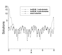
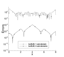
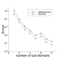
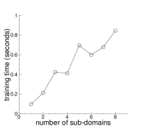
(a) (b) (c) (d)

Figure 1: Effect of the number of sub-domains, with fixed degrees of freedom per sub-domain (1D Helmholtz equation): Profiles of (a) the locELM solutions and (b) their absolute errors, computed using one sub-domain and four sub-domains. (c) The maximum and rms errors in the domain, and (d) the neural-network training time, as a function of the number of sub-domains.

We solve this problem using the locELM method presented in Section 2.2.1, by restricting the scheme to one spatial dimension. We partition $[a,b]$ into $N_{e}$ uniform sub-domains (sub-intervals), and impose the $C^{1}$ continuity conditions across the sub-domain boundaries. Let $Q$ denote the number of collocation points within each sub-domain, and consider three types of collocation points: uniform grid points, the Gauss-Lobatto-Legendre quadrature points, and random points. The majority of tests reported below are performed with uniform collocation points in each sub-domain.

For the majority of tests in this subsection, each local neural network consists of an input layer with one node (representing $x$), an output layer with one node (representing the solution $u$), and one hidden layer in between. We have also considered local neural networks with two or three hidden layers between the input and the output layers. We employ $\tanh$ as the activation function for all the hidden layers. The output layer contains no bias and no activation function, as discussed in Section 2.1. Additionally, an affine mapping operation that normalizes the input $x$ data on each sub-domain to the interval $[-1,1]$ is incorporated into the local neural networks right behind the input layer. This operation is implemented using the “lambda” layer in Keras, which contains no adjustable parameters and we do not count it toward the number of hidden layers. Following Section 2, let $M$ denote the number of nodes in the last hidden layer, which is also the number of training parameters for each sub-domain. As discussed in Section 2.1, the weight and bias coefficients in the hidden layers are pre-set to uniform random values generated on the interval $[-R_{m},R_{m}]$ and are fixed in the computation.

The main simulation parameters with locELM include the number of sub-domains ($N_{e}$), the number of collocation points per sub-domain ($Q$), the number of training parameters per sub-domain ($M$), the maximum magnitude of the random coefficients ($R_{m}$), the number of hidden layers in the local neural network, and the type of collocation points in each sub-domain. We will use the total number of collocation points ($N_{e}Q$) and the total number of training parameters ($N_{e}M$) to characterize the total degrees of freedom in the simulation. The effects of the above parameters on the simulation results will be investigated. To make the numerical tests repeatable, all the random numbers are generated by the Tensorflow library, and we employ a fixed seed value $1$ for the random number generator with all the tests in this sub-section.

Figure 1 illustrates the effect of the number of sub-domains in the locELM simulation, with the degrees of freedom per sub-domain (i.e. the number of collocation points and the number of training parameters per sub-domain) fixed. Figures 1(a) and (b) show the solution and error profiles obtained with one sub-domain and $4$ sub-domains in the locELM simulation. Figure 1(c) shows the maximum ($L^{\infty}$) and the rms ($L^{2}$) errors of the locELM solution in the overall domain as a function of the number of sub-domains. Figure 1(d) shows the training time of the overall neural network as a function of the number of sub-domains. Here the error refers to the absolute value of the difference between the locELM solution and the exact solution give by equation (33). As discussed before, the training time refers to the total computation time of the locELM method, and includes the time for computing the output of the last hidden layer $V_{j}^{s}(x)$ ($1\leqslant s\leqslant N_{e}$, $1\leqslant j\leqslant M$) and its derivatives, the coefficient matrix and the right hand side, and for solving the linear least squares problem. In this set of tests, we have employed $Q=50$ uniform collocation points per sub-domain and $M=50$ training parameters per sub-domain. Each local neural network contains a single hidden layer, and we have employed $R_{m}=3.0$ when generating the random weight/bias coefficients for the hidden layers of the local neural networks. It can be observed that the locELM method produces dramatically (nearly exponentially) more accurate results with increasing number of sub-domains, with the maximum error in the domain reduced from around $10^{1}$ for a single sub-domain to about $10^{-7}$ for $8$ sub-domains. The training time for the neural network, on the other hand, increases approximately linearly with increasing sub-domains, with the training time from about $0.1$ seconds for a single sub-domain to about $0.8$ seconds for 8 sub-domains.

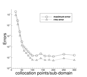
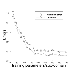
(a) (b)

Figure 2: Effect of the number of collocation points and training parameters (1D Helmholtz equation): the maximum and rms errors as a function of (a) the number of collocation points/sub-domain, and (b) the number of training parameters/sub-domain. Two uniform sub-domains are used.

Figure 2 illustrates the effects of the number of collocation points and the number of training parameters per sub-domain on the simulation accuracy. Figure 2(a) depicts the maximum and rms errors in the domain versus the number of collocation points/sub-domain. Figure 2(b) depicts the maximum and rms errors in the domain versus the number of training parameters/sub-domain. In these tests we have employed $N_{e}=2$ uniform sub-domains, uniform collocation points in each sub-domain, one hidden layer in each local neural network, and $R_{m}=3.0$ when generating the random weight/bias coefficients for the hidden layer. For the tests in plot (a) the number of training parameters/sub-domain is fixed at $M=200$, and for the tests in plot (b) the number of collocation points/sub-domain is fixed at $Q=100$. Increasing the collocation points per sub-domain causes an exponential decrease in the numerical errors initially. The errors then stagnate as the number of collocation points/sub-domain exceeds a certain point ($Q\sim 100$ in this case). The error stagnation is due to the fixed number of training parameters/sub-domain ($M=200$) here. The number of training parameters/sub-domain appears to have a similar effect on the errors. Increasing the training parameters per sub-domain also causes a nearly exponential decrease in the errors initially. The errors then stagnate as the number of training parameters increases beyond a certain point ($M\sim 175$ in this case).

The results in Figures 1 and 2 show that the current locELM method exhibits a clear sense of convergence with respect to the degrees of freedom. The numerical errors decrease exponentially or nearly exponentially, as the number of sub-domains, or the number of collocation points per sub-domain, or the number of training parameters per sub-domain increases.

Figure 3: Effect of the collocation-point distribution (1D Helmholtz equation): the maximum error in the domain versus the number of collocation points/sub-domain, obtained with three collocation-point distributions: uniform points, quadrature points, and random points.

Figure 3 illustrates the effect of the collocation-point distribution on the simulation accuracy. It shows the maximum error in the domain versus the number of collocation points/sub-domain in the locELM simulation using three types of collocation points: uniform regular points, Gauss-Lobatto-Legendre quadrature points, and random points (see Remark 2.4). In this group of tests we have employed two sub-domains ($N_{e}=2$) with $M=200$ training parameters/sub-domain, and the local neural networks each contains a single hidden layer with $R_{m}=3.0$ when generating the random weight/bias coefficients. With the same number of collocation points, we observe that the results corresponding to the random collocation points are the least accurate. The results obtained with the quadrature points are the most accurate among the three, whose errors can be orders of magnitude smaller than those with the random collocation points. The accuracy corresponding to the uniform regular collocation points lies between the other two. With the quadrature points, however, we have encountered practical difficulties in our implementation when the number of quadrature points becomes larger (above $100$), because the library our implementation is based on is unable to compute the quadrature points accurately when the number of quadrature points exceeds $100$ due to an inherent limitation. Consequently, we are unable to obtain results with more than $100$ collocation points/sub-domain when quadrature points are used, which hampers our ability to perform certain types of tests. Therefore, the majority of locELM simulations in the current work are conducted with uniform collocation points.

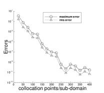
(a) (b) (c)

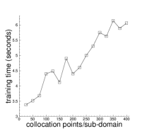
Figure 4: locELM simulations with 2 hidden layers in local neural networks (1D Helmholtz equation): profiles of (a) the locELM solutions and (b) their absolute errors, computed with $30$ and $200$ uniform collocation points per sub-domain. (c) the maximum and rms errors in the domain, and (d) the training time, as a function of the number of uniform collocation points per sub-domain.

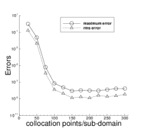
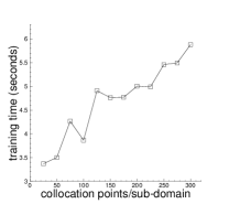
(a) (b) (c) (d)

Figure 5: locELM simulations with 3 hidden layers in local neural networks (1D Helmholtz equation): profiles of (a) the locELM solutions and (b) their absolute errors, computed with $30$ and $200$ uniform collocation points per sub-domain. (c) the maximum and rms errors in the domain, and (d) the training time, as a function of the number of uniform collocation points per sub-domain.

The test results discussed so far are obtained using a single hidden layer in the local neural networks. Traditional studies of global extreme learning machines are confined to such a configuration, using a single hidden layer in the neural network HuangZS2006 . With the current locELM method, it is observed that using more than one hidden layer in the local neural networks one can also obtain accurate results. This is demonstrated by the results in Figures 4 and 5. Figure 4 shows locELM simulation results obtained with 2 hidden layers in each of the local neural networks, and Figure 5 shows locELM results obtained with 3 hidden layers in the local neural networks. In these tests two uniform sub-domains ($N_{e}=2$) have been used. The local neural networks corresponding to Figure 4 each contains 2 hidden layers with $20$ and $300$ nodes, respectively, and $R_{m}=3.0$ is employed when the random weight/bias coefficients for the hidden layers are generated. The local neural networks corresponding to Figure 5 each contains 3 hidden layers with $20$, $20$ and $300$ nodes, respectively, and $R_{m}=1.0$ is employed when the random weight/bias coefficients are generated for the hidden layers. The number of training parameters per sub-domain in these tests is therefore fixed at $M=300$, which corresponds to the number of nodes in the last hidden layer. We have used $\tanh$ as the activation function for all the hidden layers. Uniform collocation points have been used in each sub-domain, and the number of collocation points is varied in the tests. In each of these two figures, the plots (a) and (b) are profiles of the locELM solutions and their absolute errors computed with $30$ and $200$ uniform collocation points per sub-domain, respectively. The plots (c) and (d) show the maximum/rms errors in the domain and the training time as a function of the number of collocation points per sub-domain, respectively. It is evident that the numerical errors decrease exponentially with increasing collocation points/sub-domain, similar to what has been observed with a single hidden layer from Figure 2(a), until the errors saturate as the number of collocation points increases beyond a certain point. With more than one hidden layer, the locELM method can similarly produce accurate results with a sufficient number of collocation points per sub-domain. The training time is also observed to increase essentially linearly with respect to the number of collocation points per sub-domain. Numerical experiments with even more hidden layers in the local neural networks suggest that the simulation tends to be not as accurate as those corresponding to one, two or three hidden layers. It appears to be harder to obtain accurate or more accurate results with even more hidden layers.

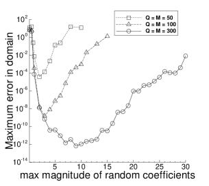
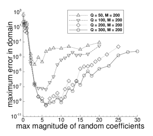
(a) (b)

Figure 6: Effect of random weight/bias coefficients in hidden layers (1D Helmholtz equation): (a) The maximum error in the domain versus $R_{m}$, for several cases with the number of collocation points/sub-domain ($Q$) and the number of training parameters/sub-domain ($M$) kept identical. (b) The maximum error in the domain versus $R_{m}$, for several cases with the number of training parameters/sub-domain fixed and the number of collocation points/sub-domain varied. Four uniform sub-domains are used in (a), and two uniform sub-domains are used in (b).

Apart from the number of collocation points and the number of training parameters in each sub-domain, we observe that the random weight/bias coefficients in the hidden layers can influence the accuracy of the locELM simulation results. As discussed in Section 2.1, the weight/bias coefficients in the hidden layers of the local neural networks are pre-set to uniform random values generated on the interval $[-R_{m},R_{m}]$, and they are fixed throughout the computation. It is observed that $R_{m}$, the maximum magnitude of the random coefficients, can influence significantly the simulation accuracy. Figure 6 demonstrates this effect with two groups of tests. In the first group, four uniform sub-domains ($N_{e}=4$) are used. The number of (uniform) collocation points per sub-domain (Q) and the number of training parameters per sub-domain ($M$) are kept to be the same, and several of these values have been considered ($Q=M=50$, $100$, $300$). Then for each of these cases we vary $R_{m}$ systematically and record the errors of the simulation results. Figure 6(a) shows the maximum error in the domain as a function $R_{m}$ for this group of tests. In the second group of tests, two uniform sub-domains ($N_{e}=2$) are used. The number of training parameters per sub-domain is fixed at $M=200$, and several values for the number of (uniform) collocation points are considered ($Q=50$, $100$, $200$, $300$). For each of these cases, $R_{m}$ is varied systematically and the corresponding errors of the simulation results are recorded. Figure 6(b) shows the maximum error in the domain as a function of $R_{m}$ for this group of tests. In both groups of tests, the local neural networks each contains a single hidden layer. These results indicate that, for a fixed simulation resolution (i.e. fixed $Q$ and $M$), the error tends be worse as $R_{m}$ becomes very large or very small. The simulation tends to produce more accurate results for a range of moderate $R_{m}$ values, which is typically around $R_{m}\approx 1\sim 10$. As the simulation resolution increases, the optimal range of $R_{m}$ values tends to expand and shift rightward (toward larger values) on the $R_{m}$ axis. Further tests also suggest that with increasing number of sub-domains the optimal range of $R_{m}$ values tends to shift leftward (toward smaller values) along the $R_{m}$ axis.

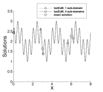
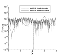
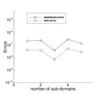
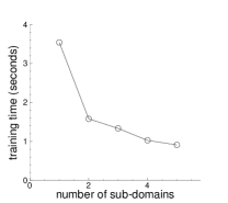
(a) (b) (c) (c)

Figure 7: Effect of the number of sub-domains, with fixed total degrees of freedom in the domain (1D Helmholtz equation): profiles of (a) the locELM solutions and (b) their absolute errors, computed using one and four uniform sub-domains in the simulation. (c) The maximum and rms errors in the domain, and (d) the training time, as a function of the number of uniform sub-domains.

We observe that the use of multiple sub-domains and local extreme learning machines can significantly accelerate the computation and reduce the network training time, without seriously compromising the accuracy, when compared with global extreme learning machines. This point is demonstrated by Figure 7. Here we fix the total degrees of freedom in the domain, i.e. the total number of collocation points and the total number of training parameters in the domain, and vary the number of sub-domains in the locELM simulation. The locELM case with a single sub-domain is equivalent to a global ELM. The total number of collocation points in the domain is fixed at $N_{e}Q=200$, and the total number of training parameters is fixed at $N_{e}M=400$. Uniform sub-domains are employed in these tests, with uniform collocation points in each sub-domain. So with multiple sub-domains the total degrees of freedom are evenly distributed to different sub-domains and local neural networks. The local neural networks each contains a single hidden layer, and the maximum magnitudes of the random coefficients ($R_{m}$) employed in the tests here are approximately in their optimal range of values. Figures 7(a) and (b) illustrates profiles of the localELM solutions and their absolute errors obtained using a single sub-domain ($Q=200$, $M=400$, $R_{m}=6.0$) and using four sub-domains ($Q=50$, $M=100$, $R_{m}=3.0$) in the locELM simulations. Both simulations have produced accurate results, with comparable error levels. Figure 7(c) shows the maximum and rms errors in the domain versus the number of sub-domains in the simulations, and Figure 7(d) shows the training time as a function of the number of sub-domains. It can be observed that the error levels corresponding to multiple sub-domains are comparable to, or in certain cases maybe slightly better or worse than, those of a single sub-domain. But the training time of the neural network is dramatically reduced with multiple sub-domains, when compared with a single sub-domain. The reduction in the training time is due to the fact that, with multiple sub-domains, the coefficient matrix in the linear least squares problem becomes very sparse, because only neighboring sub-domains are coupled through the $C^{k}$ continuity conditions while those sub-domains that are not adjacent to each other are not coupled. On the other hand, with a single sub-domain, all the degrees of freedom in the domain are coupled with one another, leading to a dense coefficient matrix in the linear least squares problem and larger computation time. These results suggest that, when compared with global ELM, the use of domain decomposition and local neural networks can reduce the coupling among the degrees of freedom in different sub-domains without seriously compromising the accuracy, and this can significantly reduce the computation time for the least squares problem, and hence the network training time.

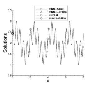
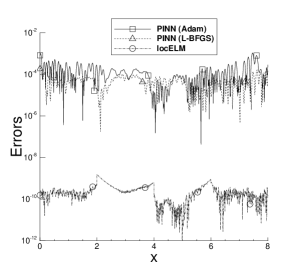
(a) (b)

Figure 8: Comparison between locELM and PINN (1D Helmholtz equation): profiles of (a) the solutions and (b) their absolute errors, obtained using PINN RaissiPK2019 with the Adam and L-BFGS optimizers, and using the current locELM method.

method	maximum error	rms error	epochs/iterations	training time (seconds)
PINN (Adam)	$1.06e-3$	$1.57e-4$	$45,000$	$507.7$
PINN (L-BFGS)	$1.98e-4$	$3.15e-5$	$22,500$	$1035.8$
locELM	$1.56e-9$	$2.25e-10$	$0$	$1.1$

Table 1: 1D Helmholtz equation: Comparison between the current locELM method and PINN, in terms of the maximum/rms errors in the domain, the number of epochs or iterations in the training of neural networks, and the training time. The problem settings correspond to those of Figures 8.

We next compare the the current locELM method with the physics-informed neural network (PINN) RaissiPK2019 method, an often-used PDE solver based on deep neural networks. Figure 8 compares profiles of the solutions (plot (a)) and their absolute errors (plot (b)) obtained using PINN with the Adam and the L-BFGS optimizers, and using the current locELM method. In the PINN simulations, the neural network contains $6$ hidden layers with $50$ nodes and the $\tanh$ activation function in each layer, and the output layer contains no activation function. The input data consist of $300$ uniform collocation points in the domain. In the PINN/Adam simulation, the network has been trained on the input data for $45,000$ epochs, with the learning rate gradually decreasing from $0.001$ at the beginning to $2.5\times 10^{-5}$ at the end. In the PINN/L-BFGS simulation, the network has been trained for $22,500$ L-BFGS iterations. In the locELM simulation, four uniform sub-domains ($N_{e}=4$) have been used, with $M=100$ training parameters per sub-domain and $Q=100$ uniform collocation points per sub-domain. The four local neural networks each consists of one hidden layer with $M=100$ nodes and the $\tanh$ activation function, and we have employed $R_{m}=3.0$ for generating random weight/bias coefficients in the hidden layer. Figure 8 shows that both PINN and the current locELM method have captured the solution quite accurately. But the current method is considerably more accurate than PINN, by a factor of nearly five orders of magnitude in terms of the errors.

Table 1 is a further comparison of PINN and locELM in terms of the maximum/rms errors in the domain, and the computational cost (the network training time and the number of epochs or iterations). The problem setting corresponds to that of Figure 8. The current method is not only much more accurate than PINN, but also considerably cheaper in terms of the computational cost. The training time with the current locELM method is on the order of a second. In contrast, it takes over $500$ seconds to train PINN with Adam and over $1000$ seconds to train it with L-BFGS. We observe a clear superiority of the current locELM method to the PINN solver in terms of both accuracy and computational cost. These observations will be confirmed and reinforced with other problems in subsequent sections.

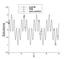
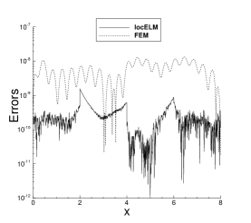
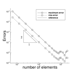
(a) (b) (c)

Figure 9: Comparison between locELM and FEM (1D Helmholtz equation): Profiles of (a) the solutions and (b) their absolute errors, computed using the finite element method (FEM) and the current locELM method. (c) The maximum and rms errors in the domain versus the number of elements from the FEM simulations, showing its second-order convergence rate.

method	elements	sub-domains	$Q$	$M$	maximum error	rms error	wall time (seconds)
locELM	–	$4$	$100$	$75$	$4.02e-8$	$5.71e-9$	$0.67$
	–	$4$	$100$	$100$	$1.56e-9$	$2.25e-10$	$1.1$
	–	$4$	$100$	$125$	$1.42e-10$	$2.55e-11$	$1.3$
FEM	$25,000$	–	–	–	$6.82e-8$	$1.74e-8$	$0.32$
	$50,000$	–	–	–	$1.67e-8$	$4.35e-9$	$0.62$
	$100,000$	–	–	–	$1.33e-8$	$3.30e-9$	$1.24$

Table 2: 1D Helmholtz equation: Comparison between the current locELM method and the finite element method (FEM), in terms of the maximum/rms errors in the domain and the training or computation time. The problem settings correspond to those of Figure 9.

Finally we compare the current locELM method with the classical finite element method (FEM). We observe that the computational performance of locELM is comparable to that of FEM, and oftentimes the locELM performance surpasses that of FEM, in terms of the accuracy and computational cost. Figures 9(a) and (b) are comparisons of the solution profiles and the error profiles obtained using locELM and FEM. Figure 9(c) shows the maximum and rms errors as a function of the number of elements obtained using FEM, demonstrating its second-order convergence rate. As mentioned before, the finite element method is implemented in Python using the FEniCS library. In these tests uniform linear elements have been used. For the plots (a) and (b), $100,000$ elements are used in the FEM simulation. In the locELM simulation, we have employed $N_{e}=4$ uniform sub-domains, $Q=100$ uniform collocation points per sub-domain, $M=100$ training parameters per sub-domain, a single hidden layer in the local neural networks, and $R_{m}=3.0$ when generating the random coefficients. It is evident that both FEM and locELM produce accurate solutions.

Table 2 provides a more comprehensive comparison between locELM and FEM for the 1D Helmholtz equation, with regard to the accuracy and computational cost. Here we list the maximum and rms errors in the domain, and the training or computation time, obtained using locELM and FEM corresponding to several numerical resolutions. The data show that the current locELM method is very competitive compared with FEM. For example, the locELM case with $M=75$ training parameters/sub-domain is similar in performance to the FEM case with $50,000$ elements, with comparable values for the numerical errors and the wall time. The locELM cases with $M=100$ and $M=125$ training parameters/sub-domain have wall time values comparable to the FEM case with $100,000$ elements, but the numerical errors of these locELM cases are considerably smaller than those of the FEM case.

3.2 Advection Equation

We next test the locELM method using the advection equation in one spatial dimension plus time, and we will demonstrate the capability of the method, when combined with the block time-marching strategy, for long-time simulations. Consider the spatial-temporal domain, $\Omega=\{(x,t)\ |\ x\in[a_{1},b_{1}],\ t\in[0,t_{f}]\}$, and the initial/boundary-value problem with the advection equation on this domain,

$$\frac{\partial u}{\partial t}-c\frac{\partial u}{\partial x}=0,$$ (34a)

$$u(a_{1},t)=u(b_{1},t),$$ (34b)

$$u(x,0)=h(x)$$ (34c)

where $u(x,t)$ is the field function to be solved for, the constant $c$ denotes the wave speed, and we impose the periodic boundary condition on the spatial domain boundaries $x=a_{1}$ and $b_{1}$. $h(x)$ denotes the initial wave profile given by

$$h(x)=2\operatorname{sech}\left[\frac{3}{\delta_{0}}\left(x-x_{0}\right)\right],$$ (35)

where $x_{0}$ is the peak location of the wave and $\delta_{0}$ is a constant that controls the width of the wave profile. The above equations and the domain specification contain several constant parameters, and we employ the following values in this problem,

$$a_{1}=0,\quad b_{1}=5,\quad c=-2,\quad\delta_{0}=1,\quad x_{0}=2.5,\quad t_{f}=2,\ \text{or}\ 10,\ \text{or}\ 100.$$ (36)

The temporal domain size $t_{f}$ is varied in different tests and will be specified in the discussions below. This problem has the following solution

$$u(x,t)=2\operatorname{sech}\left[\frac{3}{\delta_{0}}\left(-\frac{L_{1}}{2}+\xi\right)\right],\quad\xi=\bmod\left(x-x_{0}+ct+\frac{L_{1}}{2},L_{1}\right),\quad L_{1}=b_{1}-a_{1},$$ (37)

where $\bmod$ denotes the modulo operation.

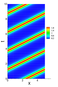
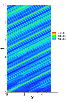
(a) (b)

Figure 10: Advection equation: Distributions of (a) the locELM solution and (b) its absolute error in the spatial-temporal plane. The temporal domain size is $t_{f}=10$, and $10$ time blocks are used in the simulation.

We simulate this problem using the locELM method together with the block time-marching strategy from Section 2.2.2, by restricting the method to one spatial dimension. We divide the overall spatial-temporal domain into $N_{b}$ uniform blocks along the temporal direction, with a time block size $\Gamma=\frac{t_{f}}{N_{b}}$. The spatial-temporal domain of each time block is then partitioned into $N_{x}$ uniform sub-domains along the $x$ direction and $N_{t}$ uniform sub-domains in time, leading to $N_{e}=N_{x}N_{t}$ uniform sub-domains in each time block. $C^{0}$ continuity is imposed on the sub-domain boundaries in both the $x$ and $t$ directions. Within each sub-domain, let $Q_{x}$ denote the number of uniform collocation points along the $x$ direction and $Q_{t}$ denote the number of uniform collocation points in time, leading to $Q=Q_{x}Q_{t}$ uniform collocation points in each sub-domain.

The local neural network corresponding to each sub-domain contains an input layer of two nodes (representing $x$ and $t$), a single hidden layer with $M$ nodes and the $\tanh$ activation function, and an output layer (representing the solution $u$) of a single node. The output layer is linear and contains no bias. An additional affine mapping normalizing the input $x$ and $t$ data to the interval $[-1,1]\times[-1,1]$ has been incorporated into the local neural networks right behind the input layer for each sub-domain. The number of training parameters per sub-domain corresponds to $M$, the width of the hidden layer. The weight and bias coefficients in the hidden layer are pre-set to uniform random values generated on $[-R_{m},R_{m}]$, as in the previous section.

The locELM simulation parameters include the number of sub-domains ($N_{x}$, $N_{t}$, $N_{e}$), the number of collocation points per sub-domain ($Q_{x}$, $Q_{t}$, $Q$), the number of training parameters per sub-domain ($M$), and the maximum magnitude of the random coefficients ($R_{m}$). The degrees of freedom within a sub-domain are characterized by ($Q,M$). The degrees of freedom in each time block are characterized by ($N_{e}Q$, $N_{e}M$). We use a fixed seed value $1$ for the Tensorflow random number generators in all the tests of this sub-section, so that all the numerical tests here are repeatable.

Figure 10 illustrates the solution from the locELM simulation. Plotted here are the distributions of the locELM solution and its absolute error in the spatial-temporal plane. In this test, the temporal domain size is $t_{f}=10$, and we employ $10$ uniform time blocks ($N_{b}=10$) in this domain. Within each time block, we have employed $N_{e}=8$ uniform sub-domains (with $N_{x}=4$ and $N_{t}=2$), and $Q=20\times 20$ uniform collocation points ($Q_{x}=Q_{t}=20$) in each sub-domain. We employ $M=300$ training parameters per sub-domain, and $R_{m}=1.0$ when generating the random weight/bias coefficients. It is evident that the current method has captured the wave solution accurately.

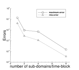
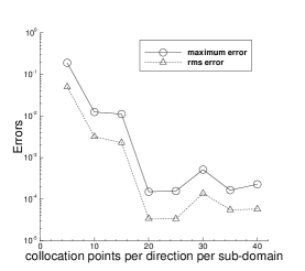
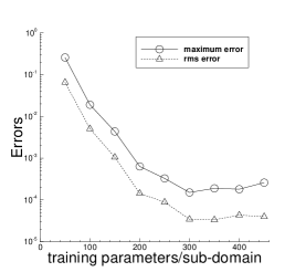
(a) (b) (c)

Figure 11: Effect of the degrees of freedom (advection equation): the maximum and rms errors in the overall domain as a function of (a) the number of sub-domains, (b) the number of collocation points in each direction per sub-domain, and (c) the number of training parameters per sub-domain. Temporal domain size is $t_{f}=10$, and $10$ time blocks have been used. In (a), the degrees of freedom per sub-domain are fixed. In (b) and (c), $N_{e}=8$ sub-domains per time block are used.

The effect of the degrees of freedom on the simulation accuracy is illustrated by Figure 11. In this group of tests, the temporal domain size is fixed at $t_{f}=10$. We have employed $N_{b}=10$ uniform time blocks within the domain, one hidden layer in each local nueral network, and $R_{m}=1.0$ when generating the random weight/bias coefficients for the hidden layers. Figure 11(a) illustrates the effect of the number of sub-domains per time block, when the degrees of freedom per sub-domain are fixed. Here the number of sub-domains within each time block is varied systematically. We employ a fixed set of $Q=20\times 20$ uniform collocation points per sub-domain ($Q_{x}=Q_{t}=20$), and fix the number of training parameters per sub-domain at $M=300$. This plot shows the maximum and rms errors in the domain as a function of the number of sub-domains per time block. Here the case with $N_{e}=2$ sub-domains/time-block corresponds to $(N_{x},N_{t})=(2,1)$. The case with $N_{e}=4$ sub-domains corresponds to $(N_{x},N_{t})=(2,2)$, and the case with $N_{e}=8$ sub-domains corresponds to $(N_{x},N_{t})=(4,2)$. It can be observed that, with increasing sub-domains/time-block, the rate of reduction in the errors, while not very regular, is approximately exponential.

Figure 11(b) shows the maximum and rms errors in the entire spatial-temporal domain as a function of the number of collocation points in each direction (with $Q_{x}=Q_{t}$ maintained) in each sub-domain. Figure 11(c) shows the maximum and rms errors in the entire domain as a function of the number of training parameters per sub-domain. In these tests, we have employed $8$ sub-domains ($N_{x}=4$, $N_{t}=2$) per time block. For those tests of Figure 11(b), the number of training parameters/sub-domain is fixed at $M=300$. For the tests of Figure 11(c), the number of collocation points/sub-domains is fixed at $Q=20\times 20$ ($Q_{x}=Q_{t}=20$). With the increase of the collocation points in each direction, or the increase of the training parameters per sub-domain, we can observe an approximately exponential decrease in the maximum and rms errors. When the number of collocation points (or training parameters) increases above a certain point, the errors start to stagnate, apparently because of the fixed number of training parameters (or the fixed number of collocation points) in these tests. The sense of convergence exhibited by the current locELM method is unmistakable.

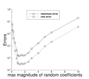
Figure 12: Effect of the random coefficients (advection equation): the maximum and rms errors in the domain as a function of $R_{m}$, the maximum magnitude of the random coefficients in hidden layer of local neural networks.

The effect of the random coefficients in the hidden layers of the local neural networks on the simulation accuracy is illustrated in Figure 12. This plot shows the maximum and rms errors in the domain as a function of $R_{m}$, the maximum magnitude of the random weight/bias coefficients. In this set of experiments, the temporal domain size is $t_{f}=10$, and $N_{b}=10$ time blocks are used in the domain. We have employed $8$ uniform sub-domains per time block ($N_{x}=4$, $N_{t}=2$), $Q=20\times 20$ uniform collocation points per sub-domain ($Q_{x}=Q_{t}=20$), and $M=300$ training parameters per sub-domain. The weight/bias coefficients in the hidden layers of the local neural networks are set to uniform random values generated on $[-R_{m},R_{m}]$, and $R_{m}$ is varied systematically in these tests. Very large or very small values of $R_{m}$ have an adverse effect on the simulation accuracy. Better accuracy generally corresponds to a range of moderate $R_{m}$ values.

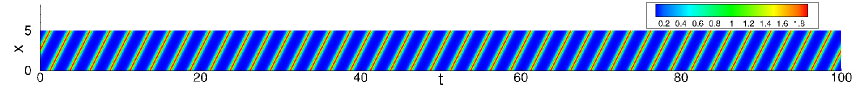
(a)

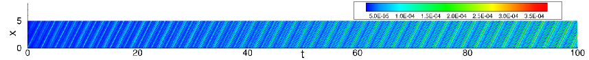
(b)

Figure 13: Long-time simulation of the advection equation: distributions of (a) the locELM solution and (b) its absolute error in the spatial-temporal plane for a long-time simulation. In these tests $100$ time blocks in the domain and $8$ sub-domains per time block are used.

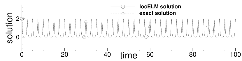
(a)

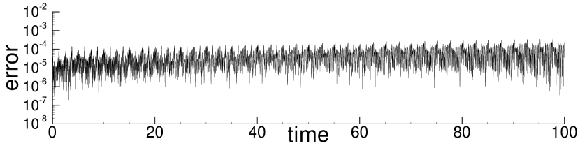
(b)

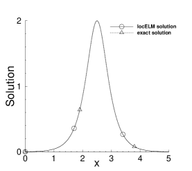
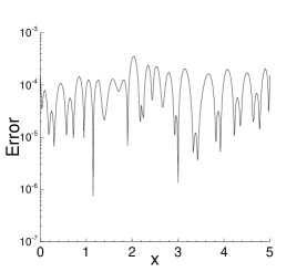
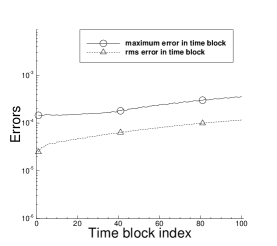
(c) (d) (e)

Figure 14: Long-time simulation of the advection equation: Time histories of the locELM solution (a) and its absolute error against the exact solution (b) at the mid-point ($x=2.5$) of the spatial domain. Profiles of the locELM solution (c) and its absolute error against the exact solution (d) at the last time instant $t=100$. (e) Time histories of the maximum and rms errors in each time block. The problem settings correspond to those of Figure 13.

Thanks to its accuracy and favorable computational cost, it is feasible to perform long-time simulations of time-dependent PDEs using the current locELM method. Figures 13 and 14 demonstrate a long-time simulation of the advection equation with the current method. In this simulation, the temporal domain size is set to $t_{f}=100$, which amounts to approximately $40$ periods of the wave propagation time. In the simulation we have employed $100$ uniform time blocks in the domain, $8$ uniform sub-domains per time block (with $N_{x}=4$ and $N_{t}=2$), $20\times 20$ uniform collocation points per sub-domain (i.e. $Q_{x}=Q_{t}=20$), $300$ training parameters per sub-domain ($M=300$), a single hidden layer in each local neural network, and $R_{m}=1.0$ when generating the random weight/bias coefficients for the hidden layers of the local neural networks. The total network training time for this locELM computation is about $892$ seconds. Figure 13 shows the distributions of the locELM solution and its absolute error in the spatial-temporal plane. Figures 14(a) and (b) are the time histories of the locELM solution and its absolute error at the mid-point ($x=2.5$) of the spatial domain. The time history of the exact solution at this point is also shown in Figure 14(a), which can be observed to overlap with that of the locELM solution. Figures 14(c) and (d) show the locELM-computed wave profile and its absolute-error profile at the last time instant $t=100$. We have also computed and monitored the maximum and rms errors of the locELM solution within each time block. Figure 14(e) shows these errors versus the time block index, which represents essentially the time histories of these block-wise maximum and rms errors. All these results show that the current method has captured the solution to the advection equation quite accurately in the long-time simulation. Accurate simulation of the advection equation in long time integration is challenging, even for classical numerical methods. The results presented here demonstrate the capability and the promise of the current method in tackling long-time dynamical simulations of these challenging problems.

(a) (b)

Figure 15: Comparison between locELM and global ELM solutions (advection equation): distributions of the absolute errors computed using the locELM method with 1 sub-domain per time block (a), which is equivalent to a global ELM, and 2 sub-domains per time block (b). Both cases have essentially the same total degrees of freedom in the domain.

In Figure 15 we compare the the solutions and their errors obtained using a single sub-domain per time block, which is equivalent to that of a global extreme learning machine, and using two sub-domains per time block in the locELM simulation. Here the temporal domain size is $t_{f}=10$, and $10$ uniform time blocks have been used in the overall domain. This figure is basically a comparison between the global ELM and locELM results. The total degrees of freedom in the overall domain are essentially the same for these two cases. In the case of 1 sub-domain/time-block, we have employed $1600$ training parameters per sub-domain and $50\times 50$ uniform collocation points per sub-domain. In the case of $2$ sub-domains/time-block we have employed $800$ training parameters per sub-domain and $35\times 35$ uniform collocation points per sub-domain. So both cases have the same total number of training parameters per time block, and also comparable total number of collocation points per time block ($2500$ for 1 sub-domain/block versus $2450$ for 2 sub-domains/block). The local neural networks contain a single hidden layer. For the case of 1 sub-domain/block we have employed $R_{m}=3.0$ when generating the random coefficients for the hidden layer of the local neural network, and for the case of $2$ sub-domains/block we have employed $R_{m}=2.0$ when generating random coefficients for the hidden layers of the local neural networks. These values are approximately in the optimal range of $R_{m}$ values for these cases. It is evident that both the locELM and the global ELM capture the wave solution quite accurately, with the locELM solution on two sub-domains/time-block better.

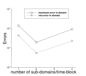
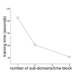
(a) (b)

Figure 16: Effect of the number of sub-domains, with fixed total degrees of freedom in the domain (advection equation): (a) the maximum and rms errors in the overall domain, and (b) the training time, as a function of the number of sub-domains per time-block. 10 time blocks are used in the domain. For all cases, the total number of training parameters per time block is fixed at $2500$, and the total number of collocation points per time block is approximately $2500$.

Figure 16 provides a comparison between the locELM and global ELM results. We fix the total degrees of freedom in each time block (temporal dimension $t_{f}=10$, $10$ time blocks, $1600$ training parameters/time-block, approximately $2500$ collocation points/time-block), and vary the number of sub-domains per time block. Figure 16(a) shows the maximum and rms errors in the overall spatial-temporal domain as a function of the number of sub-domains per time block. For the case with $4$ sub-domains per time-block, we have employed the configuration of $N_{x}=4$ and $N_{t}=1$, $M=400$ training parameters per sub-domain, $Q=25\times 25$ uniform collocation points per sub-domain, and $R_{m}=2.0$ when generating the random coefficients in the hidden layers of the local neural networks. The error levels with one sub-domain and multiple sub-domains per time block are observed to be comparable, with the results of $2$ sub-domains per time block more accurate than the others. Figure 16(b) compares the network training time corresponding to different sub-domains. The use of multiple sub-domains is observed to significantly reduce the training time of the neural network, from around $105$ seconds with a single sub-domain per time block to around $40$ seconds with $4$ sub-domains per time block. The results here confirm what has been observed in the previous section. With the same total degrees of freedom in the domain, the use of multiple sub-domains and local neural networks with the current locELM method can significantly reduce the training/computation time, while producing results with comparable accuracy when compared with the global ELM method.

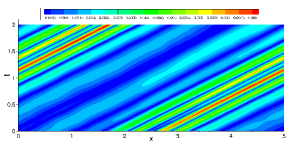
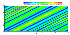
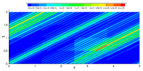
(a) (b) (c)

Figure 17: Comparison between locELM and DGM (advection equation): distributions of the absolute errors, computed using the deep Galerkin method (DGM) SirignanoS2018 with the Adam optimizer (a) and the L-BFGS optimizer (b), and computed using the current locELM method (c).

method	maximum error	rms error	epochs/iterations	training time (seconds)
DGM (Adam)	$8.37e-3$	$1.64e-3$	$60,000$	$2527.8$
DGM (L-BFGS)	$2.59e-3$	$5.37e-4$	$12,000$	$1675.9$
locELM (no block time-marching)	$2.74e-4$	$6.05e-5$	$0$	$43.4$
locELM (with block time-marching)	$1.83e-4$	$4.34e-5$	$0$	$19.3$

Table 3: Advection equation: comparison between locELM and DGM. The problem settings correspond to those of Figure 17. The two DGM cases and the locELM case with no block time-marching correspond to those of Figure 17. In the locELM case with block time-marching, two time blocks in the domain and $8$ sub-domains per time block are used. The total degrees of freedom for this case are identical to those of the locELM case with no block time marching.

Finally we compare the current locELM method with the deep Galerkin method (DGM) SirignanoS2018 , another often-used DNN-based PDE solver, for solving the advection equation. Figure 17 shows distributions of the solutions and their absolute errors obtained using DGM with the Adam and the L-BFGS optimizers and using the current locELM method. The temporal domain size is $t_{f}=2.0$ in these tests. With DGM, four hidden layers with a width of $40$ nodes and the $\tanh$ activation function in each layer have been employed in the neural networks. When computing the residual norms in the DGM loss function, we have partitioned the domain into $8$ sub-regions ($4$ in $x$ and $2$ in time) and used $30\times 30$ Gaussian quadrature points in each sub-region for calculating the integrals. The periodic boundary condition is enforced exactly using the method from DongN2020 for DGM. With the Adam optimizer, the neural network has been trained for $60,000$ epochs, with the learning rate decreasing gradually from $0.001$ at the beginning to $2.5\times 10^{-5}$ at the end of training. With the L-BFGS optimizer, the neural network has been trained for $12,000$ iterations. In the locELM simulation, a single time block has been used in the spatial-temporal domain, i.e. without block time marching. We employ $16$ sub-domains (with $4$ sub-domains in $x$ and time) per time block, $20\times 20$ uniform collocation points in each sub-domain, $250$ training parameters per sub-domain, a single hidden layer in each local neural network, and $R_{m}=2.0$ for generating the random weight/bias coefficients for the hidden layer of the local neural networks. One can observe that the current method produces considerably more accurate result than DGM for the advection equation.

Table 3 provides further comparisons between locELM and DGM. Here we list the maximum and rms errors in the overall spatial-temporal domain, the number of epochs or iterations in the network training, and the training time obtained using DGM (Adam/L-BFGS optimizers) and using locELM without block time marching, and additionally using locELM together with block time marching. The problem settings here correspond to those of Figure 17, and the DGM cases and the locELM case without block time marching correspond to those in Figure 17. In the locELM case with block time marching, we have employed $2$ uniform time blocks in the spatial-temporal domain, $8$ sub-domains ($N_{x}=4$, $N_{t}=2$) per time block, $20\times 20$ uniform collocation points per sub-domain, $250$ training parameters per sub-domain, a single hidden layer in the local neural networks, and $R_{m}=2.0$ when generating the random weight/bias coefficients. So the total degrees of freedom in this case are identical to those of the locELM case without block time marching. The data in the table shows that the current locELM method (with and without block time marching) is much more accurate than DGM (by an order of magnitude), and is dramatically faster to train than DGM (by nearly two orders of magnitude). In addition, we observe that the locELM method with block time marching and a moderate time block size can significantly reduce the training time, and simultaneously achieve the same or better accuracy, when compared with that without block time marching.

3.3 Diffusion Equation

In this subsection we the test the locELM method using the diffusion equation in one and two spatial dimensions (plus time). Let us first study the 1D diffusion equation. We consider the spatial-temporal domain, $\Omega=\{(x,t)\ |\ x\in[a_{1},b_{1}],\ t\in[0,t_{f}]\}$, and the following initial/boundary-value problem,

$$\frac{\partial u}{\partial t}-\nu\frac{\partial^{2}u}{\partial x^{2}}=f(x,t),$$ (38a)

$$u(a_{1},t)=g_{1}(t),$$ (38b)

$$u(b_{1},t)=g_{2}(t),$$ (38c)

$$u(x,0)=h(x),$$ (38d)

where $u(x,t)$ is the field function to be solved for, $f(x,t)$ is a prescribed source term, the constant $\nu$ is the diffusion coefficient, $g_{1}(t)$ and $g_{2}(t)$ are the boundary conditions, and $h(x)$ is the initial field distribution. The values for the constant parameters involved in the above equations and in the domain specification are,

$$a_{1}=0,\quad b_{1}=5,\quad\nu=0.01,\quad t_{f}=10\ \text{or}\ 1.$$

We choose the source term $f$ such that the following function satisfies equation (38a),

$$u(x,t)=\left[2\cos\left(\pi x+\frac{\pi}{5}\right)+\frac{3}{2}\cos\left(2\pi x-\frac{3\pi}{5}\right)\right]\left[2\cos\left(\pi t+\frac{\pi}{5}\right)+\frac{3}{2}\cos\left(2\pi t-\frac{3\pi}{5}\right)\right].$$ (39)

We choose the boundary conditions $g_{1}(t)$ and $g_{2}(t)$ and the initial condition $h(x)$ according to equation (39), by restricting this expression to the corresponding boundaries of the spatial-temporal domain. Therefore, the function given by (39) solves the initial/boundary value problem represented by equations (38a)–(38d).

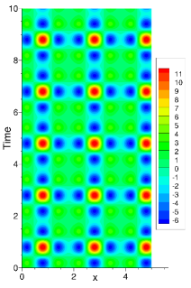
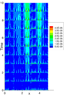
(a) (b)

Figure 18: 1D diffusion equation: distributions of the solution (a) and its absolute error (b) computed using the current locELM method. 10 time blocks and 5 sub-domains per time block are employed.

We employ the locELM method together with block time marching from Section 2.2.2 to solve this initial/boundary value problem, by restricting the method to one spatial dimension. We partition the spatial-temporal domain $\Omega$ in time into $N_{b}$ uniform blocks, and compute these time blocks individually and successively. Within each time block, we further partition its spatial-temporal domain into $N_{x}$ uniform sub-domains along the $x$ direction and $N_{t}$ uniform sub-domains in time, leading to $N_{e}=N_{x}N_{t}$ uniform sub-domains per time block. We impose $C^{1}$ continuity conditions on the sub-domain boundaries in the $x$ direction and $C^{0}$ continuity on the sub-domain boundaries in the temporal direction. Within each sub-domain we use $Q_{x}$ uniform collocation points along the $x$ direction and $Q_{t}$ uniform collocation points in time as the input training data, leading to a total of $Q=Q_{x}Q_{t}$ uniform collocation points per sub-domain.

We use one local neural network to approximate the solution on each sub-domain within the time block, thus leading to a total of $N_{e}$ local neural networks in the locELM simulation. In the majority of tests of this subsection the local neural networks each contains a single hidden layer with $M$ nodes and the $\tanh$ activation function. We also report results obtained with the local neural networks containing more than one hidden layer. The input layer of the local neural networks consists of two nodes, representing $x$ and $t$. The output layer consists of a single node, representing the solution $u$, and has no bias coefficient and no activation function. As in previous subsections, we incorporate an additional affine mapping operation right behind the input layer of the local neural network to normalize the input $x$ and $t$ data to the interval $[-1,1]\times[-1,1]$ in each sub-domain. The weight/bias coefficients in the hidden layer of each of the local neural networks are set to uniform random values generated on the interval $[-R_{m},R_{m}]$. We use a fixed seed value $22$ for the Tensorflow random number generator for all the tests in this subsection.

The locELM simulation parameters include the number of time blocks ($N_{b}$), the number of sub-domains per time block ($N_{e},N_{x},N_{t}$), the number of training parameters per sub-domain ($M$), the number of collocation points per sub-domain ($Q_{x}$, $Q_{t}$, $Q$), and the maximum magnitude of the random coefficients ($R_{m}$). In accordance with previous subsections, we use $(Q,M)$ to characterize the degrees of freedom within a sub-domain, and $(N_{e}Q,N_{e}M)$ to characterize the degrees of freedom within a time block.

Figure 18 shows distributions of the locELM solution and its absolute error in the spatial-temporal plane. In this test the temporal domain size is set to $t_{f}=10$. We have employed $N_{b}=10$ uniform time blocks in the simulation, $N_{e}=5$ uniform sub-domains per time block (with $N_{x}=5$ and $N_{t}=1$), $Q=30\times 30$ uniform collocation points in each sub-domain (with $Q_{x}=Q_{t}=30$), $M=300$ training parameters per sub-domain, a single hidden layer in the local neural networks, and $R_{m}=1.0$ when generating the random weight/bias coefficients for the hidden layers of the local neural networks. It is evident that the locELM method has captured the solution very accurately, with the absolute error on the order of $10^{-9}\sim 10^{-8}$.

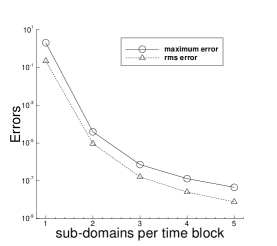
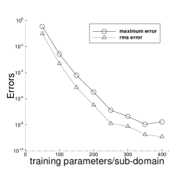
(a) (b) (c)

Figure 19: Effect of the degrees of freedom on simulation accuracy (1D diffusion equation): the maximum and rms errors in the domain as a function of (a) the number of sub-domains in each time block, (b) the number of collocation points in each direction in each sub-domain, and (c) the number of training parameters in each sub-domain. Temporal domain size is $t_{f}=10$ and $10$ uniform time blocks are used.

The effect of the degrees of freedom on the simulation accuracy is illustrated by Figure 19. In this group of tests, the temporal domain size is set to $t_{f}=10$, and we have employed $N_{b}=10$ uniform time blocks in the spatial-temporal domain, a single hidden layer in each local neural network, and $R_{m}=1.0$ when generating the random coefficients for the hidden layers of the local neural networks. The number of sub-domains in each time block, or the number of collocation points per sub-domain, or the number of training parameters per sub-domain has been varied in the tests.

Figure 19(a) illustrates the effect of the number of sub-domains within each time block, while the degrees of freedom per sub-domain are fixed. Here we fix the number of uniform collocation points per sub-domain at $Q=30\times 30$ ($Q_{x}=Q_{t}=30$) and the number of training parameters per sub-domain at $M=300$, and then vary the number of uniform sub-domains per time block systematically. This plot shows the maximum and rms errors of the locELM solution in the overall spatial-temporal domain as a function of the number of sub-domains per time block in the simulations. With increasing number of sub-domains, the numerical errors are observed to decrease dramatically, from around $10^{-1}$ with one sub-domain/time-block to around $10^{-8}$ with $5$ sub-domains/time-block.

Figure 19(b) illustrates the effect of the number of collocation points per sub-domain on the simulation accuracy. Here we use $N_{e}=5$ uniform sub-domains (with $N_{x}=5$ and $N_{t}=1$) in each time block, fix the the number of training parameters per sub-domain at $M=300$, and vary the number of collocation points per sub-domain while maintaining $Q_{x}=Q_{t}$. This plot shows the maximum and rms errors in the overall spatial-temporal domain as a function of the number of collocation points in each direction in each sub-domain. The numerical errors can be observed to initially decrease exponentially with increasing number of collocation points per direction when it is below about $20$, and then stagnate at a level around $10^{-8}\sim 10^{-7}$ as the number of collocation points per direction further increases.

Figure 19(c) illustrates the effect of the number of training parameters on the simulation accuracy. Here we use $N_{e}=5$ sub-domains (with $N_{x}=5$ and $N_{t}=1$) in each time block, fix the number of collocation points per sub-domain at $Q=30\times 30$ ($Q_{x}=Q_{t}=30$), and vary the number of training parameters per sub-domain. The plot shows the maximum/rms errors in the overall domain as a function of the number of training parameters per sub-domain. One can observe that the errors initially decrease exponentially with increasing number of training parameters/sub-domain when it is below about $250$, and then the error reduction slows down as the number of training parameters/sub-domain further increases. These behaviors are consistent with what have been observed with other problems in previous subsections.

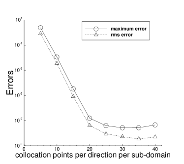
(b)

Figure 20: Results obtained with two hidden layers in local neural networks (1D diffusion equation): The maximum/rms errors in the domain versus the number of collocation points in each direction per sub-domain.

In Figure 20 we show results obtained with local neural networks containing more than one hidden layer. In this group of simulations, each local neural network contains two hidden layers, with $30$ and $300$ nodes in these two layers, respectively. The activation function is $\tanh$ in both hidden layers. The temporal domain size is $t_{f}=10$, and $10$ uniform time blocks have been used. We employ $N_{e}=5$ sub-domains per time block ($N_{x}=5$ and $N_{t}=1$), $M=300$ training parameters per sub-domain (width of the last hidden layer), and $R_{m}=0.5$ when generating the random weight/bias coefficients for the hidden layers of the local neural networks. The number of collocation points per sub-domain ($Q$) is varied systematically while $Q_{x}=Q_{t}$ is maintained. Figure 20(a) shows the distribution of the absolute error of the locELM solution in the spatial-temporal plane, obtained with $Q=30\times 30$ uniform collocation points per sub-domain. This figure can be compared with Figure 18(b), which corresponds to the same simulation resolution but is obtained with local neural networks containing a single hidden layer. Figure 20(b) shows the maximum and rms errors in the overall domain as a function of the number of collocation points in each direction per sub-domain. This figure can be compared with Figure 19(b), which corresponds to a single hidden layer in the local neural networks. It is evident that the solution has been captured accurately by the current locELM method using two hidden layers in the local neural networks. The results shown here and those results in Section 3.1 (see Figures 4 and 5) demonstrate that the current locELM method, using local neural networks with a small number of (more than one) hidden layers, is able to produce accurate simulation results.

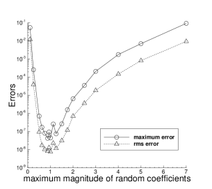
Figure 21: Effect of the random coefficients in local neural networks (1D diffusion equation): the maximum and rms errors in the domain as a function of $R_{m}$, the maximum magnitude of the random coefficients.

Figure 21 illustrates the effect of the random weight/bias coefficients in the local neural networks on the simulation accuracy. It shows the maximum and rms errors of the locELM solution in the overall domain as a function of $R_{m}$, the maximum magnitude of the random coefficients. In this group of tests, the temporal domain size is $t_{f}=10$, and we have employed $N_{b}=10$ uniform time blocks in the domain, $N_{e}=5$ uniform sub-domains per time block ($N_{x}=5$, $N_{t}=1$), $Q=30\times 30$ uniform collocation points per sub-domain, $M=300$ training parameters per sub-domain, and a single hidden layer in the local neural networks. The random coefficients in the hidden layers are generated on $[-R_{m},R_{m}]$, and $R_{m}$ is varied systematically in these tests. We observe a similar behavior to those in previous subsections. A better accuracy can be attained with a range of moderate $R_{m}$ values, while very large or very small $R_{m}$ values tend to produce less accurate results.

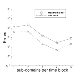
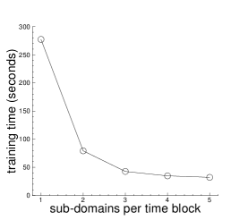
(a) (a)

Figure 22: Effect of the number of sub-domains, with fixed total degrees of freedom in the domain (1D diffusion equation): (a) the maximum and rms errors in the domain, and (b) the training time, as a function of the number of sub-domains per time block.

Figure 22 depicts a study of the effect of the number of sub-domains in the simulation on the simulation accuracy and on the network training time, while the total number of degrees of freedom in the domain is fixed. In this group of tests, the temporal domain size is $t_{f}=10$, and we have used $N_{b}=10$ time blocks in the overall spatial-temporal domain. The number of uniform sub-domains per time block is varied systematically between $N_{e}=1$ and $N_{e}=5$ in the simulations, implemented by fixing $N_{t}=1$ and varying $N_{x}$ between $1$ and $5$. We set the number of training parameters per sub-domain ($M$), and the number of uniform collocation points per sub-domain ($Q$, with $Q_{x}=Q_{t}$), in a way such that the total number of training parameters per time block is fixed at $N_{e}M=1500$ and the total number of collocation points per time block is approximately fixed at $N_{e}Q\approx 2500$. Specifically, $M$ and $Q$ in different cases are: $M=1500$ and $Q=50\times 50$ for $1$ sub-domain per time block, $M=750$ and $Q=35\times 35$ for $2$ uniform sub-domains per time block, $M=500$ and $Q=29\times 29$ for $3$ uniform sub-domains per time block, $M=375$ and $Q=25\times 25$ for $4$ uniform sub-domains per time block, and $M=300$ and $Q=22\times 22$ for $5$ uniform sub-domains per time block. We employ $R_{m}=3.0$ when generating the random coefficients for the case with one sub-domain per time block, which is approximately at the optimal range of $R_{m}$ values for this case. We employ $R_{m}=1.0$ when generating the random coefficients for the rest of the cases with $N_{e}=2\sim 5$ sub-domains per time block. Note that the case with one sub-domain per time block is equivalent to the configuration of a global ELM in the simulation. Figure 22(a) shows a comparison of the maximum and rms errors in the overall spatial-temporal domain as a function of the number of sub-domains per time block in the simulations. It can be observed that the numerical errors with $2$ or more sub-domains are comparable to or smaller than the errors corresponding to one sub-domain in the simulations. Figure 22(b) shows the neural-network training time as a function of the number of sub-domains per time block. One can observe that the training time decreases significantly with increasing number of sub-domains. Compared with the case of one sub-domain per time block, the training time corresponding to $2$ and more sub-domains in the simulations has been considerably reduced, e.g. $277$ seconds with one sub-domain versus $79$ seconds with $2$ sub-domains. These results confirm and reinforce our observations with the other problems that, compared with global ELM, the use of domain decomposition and locELM with multiple sub-domains can significantly reduce the network training time, and hence the computational cost, while attaining the same or sometimes even better accuracy in the simulation results.

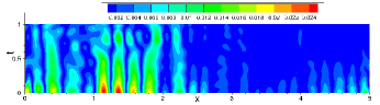
(a)

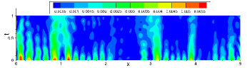
(b)

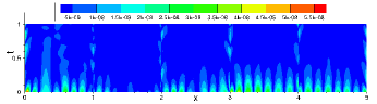
(c)

Figure 23: Comparison between locELM and DGM (1D diffusion equation): Distributions of the absolute errors computed using DGM with the Adam optimizer (a) and the L-BFGS optimizer (b) and using the current locELM method (c).

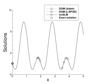
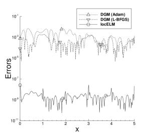
(a) (b)

Figure 24: Comparison between locELM and DGM (1D diffusion equation): Profiles of the solutions (a) and their absolute errors (b) at $t=1.0$ obtained using DGM (Adam/L-BFGS optimizers) and using the current locELM method. The problem settings and the simulation parameters correspond to those of Figure 23.

Let us now compare the current locELM method and the deep Galerkin method (DGM) for solving the 1D diffusion equation. Figure 23 compares distributions of the solutions and their absolute errors obtained using DGM with the Adam optimizer and the L-BFGS optimizer and using the current locELM method. The temporal domain size is set to $t_{f}=1$ in these tests. With DGM, the neural network consists of 4 hidden layers, with a width of $40$ nodes and the $\tanh$ activation function in each layer. When computing the loss function of the network, we have divided the domain into $5$ uniform sub-regions along the $x$ direction, and computed the residual norm integral by the Gaussian quadrature rule on $20\times 20$ Gauss-Lobatto-Legendre quadrature points in each sub-region. With the Adam optimizer, the neural network has been trained for $135,000$ epochs, with the learning rate decreasing gradually from $0.001$ at the beginning to $2.5\times 10^{-6}$ at the end of the training. With the L-BFGS optimizer, the neural network has been trained for $36,000$ L-BFGS iterations. In the simulation with the current locELM method, we employ $N_{b}=1$ time block in the spatial-temporal domain, $N_{e}=5$ sub-domains (with $N_{x}=5$, $N_{t}=1$) per time block, $Q=30\times 30$ uniform collocation points per sub-domain, $M=300$ training parameters per sub-domain, $1$ hidden layer in each of the local neural networks, and $R_{m}=1.0$ when generating the random weight/bias coefficients. The DGM has captured the solution reasonably well. But its error levels are considerably higher, by about five orders of magnitude, than that of the current locELM method ($10^{-3}$ versus $10^{-8}$).

A comparison of the solution and the error profiles between locELM and DGM is provided in Figure 24. Figure 24(a) compares the solution profiles at $t=1.0$ obtained using DGM (Adam/L-BFGS optimizers) and using the current locELM method, together with that of the exact solution. The settings and the parameters correspond to those of Figure 23. The computed profiles all agree with the exact solution quite well. Figure 24(b) compares profiles of the absolute errors at $t=1.0$ obtained with DGM and the current method. The numerical error of the current method, which is at a level around $10^{-9}$, is significantly smaller than those from DGM, which are at a level around $10^{-4}$.

method	maximum error	rms error	epochs/iterations	training time (seconds)
DGM (Adam)	$2.59e-2$	$3.84e-3$	$135,000$	$4194.5$
DGM (L-BFGS)	$5.82e-3$	$8.21e-4$	$36,000$	$3201.4$
locELM	$5.82e-8$	$6.25e-9$	$0$	$28.4$

Table 4: 1D diffusion equation: comparison between DGM (Adam/L-BFGS optimizers) and locELM. The settings and parameters correspond to those of Figure 23.

In Table 4 we provide some further comparisons between locELM and DGM in terms of the accuracy and the computational cost. Here we list the maximum and rms errors in the overall spatial-temporal domain, the number of epochs or iterations in network training, and the training time of DGM with the Adam and L-BFGS optimizers and of the current locELM method. The problem settings and the simulation parameters correspond to those of Figure 23. The data demonstrate the clear superiority of locELM to DGM, with the locELM errors five orders of magnitude smaller and the training time over two orders of magnitude less.

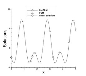
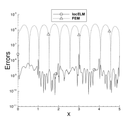
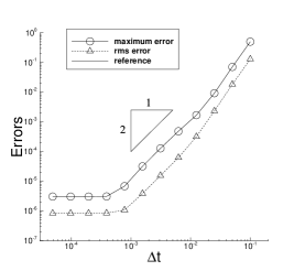
(a) (b) (c)

Figure 25: Comparison between locELM and FEM (1D diffusion equation): Profiles of (a) the solutions and (b) their absolute errors at $t=1.0$, computed using the current locELM method and using the finite element method (FEM). (c) The FEM maximum and rms errors at $t=0.5$ versus $\Delta t$, showing the temporal second-order convergence rate of FEM.

method	$\Delta t$	elements	sub-domains	$Q$	$M$	maximum	rms	wall time
						error	error	(seconds)
locELM	–	–	$5$	$20\times 20$	$200$	$2.48e-6$	$2.23e-7$	$7.9$
	–	–	$5$	$20\times 20$	$250$	$8.97e-8$	$2.25e-8$	$11.3$
	–	–	$5$	$30\times 30$	$300$	$5.82e-8$	$6.25e-9$	$28.4$
FEM	$0.002$	$2000$	–	–	–	$2.42e-4$	$4.40e-5$	$5.9$
	$0.001$	$2000$	–	–	–	$9.82e-5$	$2.01e-5$	$12.0$
	$0.0005$	$2000$	–	–	–	$1.54e-4$	$2.61e-5$	$24.0$
	$0.00025$	$2000$	–	–	–	$1.72e-4$	$2.85e-5$	$48.3$
	$0.002$	$5000$	–	–	–	$3.63e-4$	$5.98e-5$	$12.3$
	$0.001$	$5000$	–	–	–	$6.99e-5$	$1.22e-5$	$24.6$
	$0.0005$	$5000$	–	–	–	$1.69e-5$	$3.43e-6$	$48.8$
	$0.00025$	$5000$	–	–	–	$2.26e-5$	$3.91e-6$	$97.9$
	$0.002$	$10000$	–	–	–	$3.85e-4$	$6.32e-5$	$22.2$
	$0.001$	$10000$	–	–	–	$9.11e-5$	$1.49e-5$	$43.9$
	$0.0005$	$10000$	–	–	–	$1.75e-5$	$3.05e-6$	$86.9$
	$0.00025$	$10000$	–	–	–	$4.24e-6$	$8.58e-7$	$179.0$

Table 5: 1D diffusion equation: comparison between FEM and the current locELM method, in terms of the maximum/rms errors in the overall domain and the training/computation time. The temporal domain size is $t_{f}=1$. $R_{m}=1.0$ in locELM simulations.

Let us next compare the current locELM method with the classical finite element method for solving the 1D diffusion equation. In Figures 25(a) and (b) we compare profiles of the solutions and their absolute errors at $t=1.0$, obtained using the current locELM method and the finite element method. The domain and problem settings in these tests correspond to those of Figures 23(e,f), with a temporal domain size $t_{f}=1$. The simulation parameters for the locELM computation also correspond to those of Figures 23(e,f). For the FEM simulation, the diffusion equation (38a) is discretized in time by the second-order backward differentiation formula (BDF2), and the diffusion term is treated implicitly. We have employed a time step size $\Delta t=0.00025$ and $10,000$ uniform linear elements to discretize the spatial domain. It is evident from these data that both the FEM and the current method have produced accurate results. Figure 25(c) shows the maximum and rms errors at $t=0.5$ versus the time step size $\Delta t$ with FEM, showing the second-order temporal convergence rate. In these tests a fixed mesh of $10,000$ uniform linear elements has been used, which accounts for the observed error saturation in Figure 25(c) when $\Delta t$ becomes sufficiently small.

Table 5 provides a comparison of the accuracy and the computational cost of the locELM method and the finite element method. In these tests the temporal domain size is set to $t_{f}=1$. In the locELM simulations we employ a single time block in the spatial-temporal domain, $5$ uniform sub-domains in the time block, and several sets of collocation points/sub-domain and training parameters/sub-domain, a single hidden layer in the local neural networks, and $R_{m}=1.0$ when generating the random coefficients. In the FEM simulations, we employ several sets of elements and $\Delta t$ values. The maximum error and the rms error in the overall spatial-temporal domain have been computed, and the wall time for the computation or network training have been recorded. In Table 5 we list these errors and the wall time numbers corresponding to the different simulation cases with locELM and FEM. We observe that the current method performs markedly better than FEM. The current method achieves a considerably better accuracy with the same computational cost as FEM, and it incurs a lower computational cost while achieving the same accuracy as FEM. For example, the locELM case with $(Q,M)=(20\times 20,250)$ has a computational cost comparable to the FEM cases with $2000$ elements and $\Delta t=0.001$ and with $5000$ elements and $\Delta t=0.002$. But the numerical errors of locELM are considerably smaller, by around three orders of magnitude, than those of the FEM cases. The locELM case with $(Q,M)=(30\times 30,300)$ has a lower computational cost, by a factor of about three, and a considerably better accuracy, by a factor of nearly three orders of magnitude, than the FEM case with $10,000$ elements and $\Delta t=0.0005$.

3.4 Nonlinear Examples

3.4.1 Nonlinear Helmholtz Equation

As the first nonlinear example, we test the locELM method using the boundary value problem with the nonlinear Helmholtz equation in one dimension. Consider the domain $[a,b]$ and the following boundary value problem on this domain,

$$\frac{d^{2}u}{dx^{2}}-\lambda u+\beta\sin(u)=f(x),$$ (40a)

$$u(a)=h_{1},$$ (40b)

$$u(b)=h_{2},$$ (40c)

where $u(x)$ is the function to be solved for, $f(x)$ is a prescribed source term, $\lambda$ and $\beta$ are constant parameters, and $h_{1}$ and $h_{2}$ are the boundary values. We assume the following values for the constant parameters involved in these equations and domain specification,

$$a=0,\quad b=8,\quad\lambda=50,\quad\beta=10.\quad$$

We choose the source term $f(x)$ and the boundary values $h_{1}$ and $h_{2}$ such that the following function satisfies the equations (40a)–(40c),

$$u(x)=\sin\left(3\pi x+\frac{3\pi}{20}\right)\cos\left(4\pi x-\frac{2\pi}{5}\right)+\frac{3}{2}+\frac{x}{10}.$$ (41)

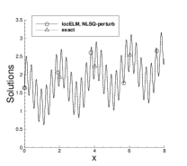
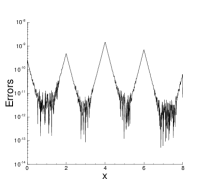
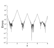
(a) (b) (c) (d)

Figure 26: Nonlinear Helmholtz equation: profiles of the locELM solutions (a,c) and their absolute errors (b,d), computed using NLSQ-perturb (a,b) and Newton-LLSQ (c,d).

We employ the locELM method discussed in Section 2.3.1 for solving this problem, by restricting the method to one dimension. We partition the domain $[a,b]$ into $N_{e}$ uniform sub-domains (sub-intervals), and impose the $C^{1}$ continuity conditions across the sub-domain boundaries. We employ $Q$ uniform collocation points within each sub-interval.

The local neural network for each sub-domain consists of an input layer with one node (representing $x$), a single hidden layer with $M$ nodes and the $\tanh$ activation function, and an output layer with one node (representing the solution $u$) and no activation function and no bias. An additional affine mapping operation normalizing the input $x$ data to the interval $[-1,1]$ is incorporated into the local neural networks right behind the input layer for each sub-domain. The weight and bias coefficients in the hidden layer of the local neural networks are set to uniform random values generated on the interval $[-R_{m},R_{m}]$. We employ a fixed seed value $12$ for the Tensorflow random generator for all the tests reported in this sub-section.

We employ the nonlinear least squared method with perturbations (NLSQ-perturb) and the combined Newton/linear least squared method (Newton-LLSQ) from Section 2.3.1 for computing the resultant nonlinear problem. The initial guess to the solution is set to zero in all the tests of this subsection. In the NLSQ-perturb method (see Algorithm 1), we have employed $\delta=0.2$, and $\xi_{2}=1$ as discussed in Remark 2.7, for generating the random perturbations in the following tests.

The locELM simulation parameters include the number of sub-domains ($N_{e}$), the number of collocation points per sub-domain ($Q$), the number of training parameters per sub-domain ($M$), and the maximum magnitude of the random coefficients of the local neural networks ($R_{m}$).

Figure 26 illustrates the profiles of the locELM solutions and their absolute errors computed using the NLSQ-perturb and Newton-LLSQ methods. In these simulations, we have employed $N_{e}=4$ uniform sub-domains, $Q=100$ uniform collocation points per sub-domain, $M=200$ training parameters per sub-domain, and $R_{m}=5.0$ for generating the random weight/bias coefficients. The profile of the exact solution given by (41) is also included in these plots. The solution profiles obtained with the current method exactly overlap with that of the exact solution. The error profiles indicate that the NLSQ-perturb method results in more accurate results than Newton-LLSQ, with error levels on the order $10^{-12}\sim 10^{-9}$ for NLSQ-perturb versus $10^{-9}\sim 10^{-5}$ for Newton-LLSQ.

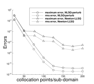
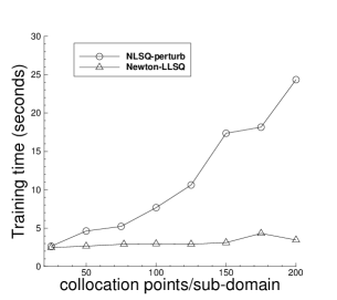
(a) (b)

Figure 27: Effect of collocation points (nonlinear Helmholtz equation): (a) the maximum and rms errors in the domain, and (b) the network training time, as a function of the number of collocation points per sub-domain, computed using the locELM method with NLSQ-perturb and Newton-LLSQ.

Figure 27 demonstrates the effect of the number of collocation points per sub-domain on the simulation accuracy and the computational cost. In this group of tests, we have employed $N_{e}=4$ sub-domains, $M=200$ training parameters per sub-domain, and $R_{m}=5.0$ when generating the random coefficients. The number of uniform collocation points per sub-domain is varied systematically between $Q=25$ and $Q=200$. Figure 27(a) shows the maximum and rms errors in the domain as a function of the number of collocation points per sub-domain, obtained with NLSQ-perturb and Newton-LLSQ. Figure 27(b) shows the corresponding training time of the overall neural network versus the number of collocation points per sub-domain. With the Newton-LLSQ method, the errors are observed to decrease gradually with increasing number of collocation points, and appear to stagnate at a level around $10^{-6}$ when the number of collocation points/sub-domain is beyond $150$. With the NLSQ-perturb method, the errors initially decrease exponentially with increasing number of collocation points (when below $125$), and then stagnate at a level around $10^{-11}$ when the number of collocation points/sub-domain increases to $150$ and beyond. The NLSQ-perturb results are in general considerably more accurate than those obtained with Newton-LLSQ. In terms of the training time, the Newton-LLSQ method is consistently faster than NLSQ-perturb, and the difference becomes larger as the number of collocation points increases. With the Newton-LLSQ method, the training time appears not sensitive to the number of collocation points, and remains nearly the same with increasing number of collocation points (Figure 27(b)). With the NLSQ-perturb method, the training time increases approximately linearly with increasing number of collocation points per sub-domain, and it becomes substantially slower than Newton-LLSQ when the number of collocation points becomes large.

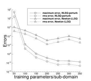
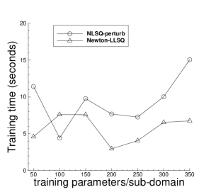
(c) (c)

Figure 28: Effect of the number of training parameters (nonlinear Helmholtz equation): (a) the maximum and rms errors in the domain, and (b) the network training time, versus the number of training parameters per sub-domain, computed using the locELM method with NLSQ-perturb and Newton-LLSQ.

Figure 28 demonstrates the effect of the number of training parameters per sub-domain on the simulation accuracy and the computational cost. In this group of tests, we have employed $N_{e}=4$ sub-domains, $Q=100$ uniform collocation points per sub-domain, and $R_{m}=5.0$ when generating the random coefficients in the hidden layers of the local neural networks. The number of training parameters per sub-domain is varied systematically between $50$ and $350$. Figure 28(a) shows the maximum and rms errors of the solutions as a function of the number of training parameters per sub-domain obtained with NLSQ-perturb and Newton-LLSQ. With NLSQ-perturb, the numerical errors decrease substantially as the number of training parameters per sub-domain increases, reaching a level around $10^{-10}$ when the number of training parameters increases beyond $200$. With Newton-LLSQ, one can also observe a decrease in the errors as the number of training parameters increases. But the error reduction is much slower. When the number of training parameters per sub-domain exceeds $200$, the errors with Newton-LLSQ no longer seem to decrease further and remain at a level around $10^{-5}$. It is evident that the results from the Newton-LLSQ method are generally much less accurate than those from the NLSQ-perturb method. Figure 28(b) shows the corresponding network training time as a function of the number of training parameters per sub-domain. In the range of training parameters tested here, the training time with both of these two methods appear to fluctuate around a certain level. But the training time with the Newton-LLSQ method is generally notably smaller than that with the NLSQ-perturb method, except for the outlier point corresponding to $100$ training parameters per sub-domain. These data suggest that Newton-LLSQ is generally faster than NLSQ-perturb.

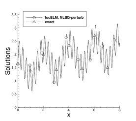
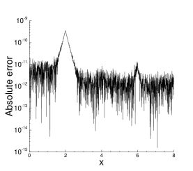
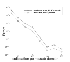
(a) (b) (c)

Figure 29: Results obtained with $2$ hidden layers in local neural networks (nonlinear Helmholtz equation): profiles of (a) the locELM (NLSQ-perturb) solution and (b) its absolute error. (c) The maximum/rms errors in the domain versus the number of collocation points per sub-domain.

With the current locELM method, the local neural network can contain more than one hidden layer. As shown in previous sub-sections, local neural networks with a small number (more than one) of hidden layers can also deliver accurate results using the current method. Figure 29 demonstrates again this point with the nonlinear Helmholtz equation. In this group of tests, we employ $N_{e}=4$ uniform sub-domains, $M=250$ training parameters per sub-domain, $2$ hidden layers (with widths $25$ and $250$, respectively, and the $\tanh$ activation function) in each local neural network, and $R_{m}=2.0$ when generating the random weight/bias coefficients for these hidden layers. The number of uniform collocation points per sub-domain is varied systematically in these tests. Figures 29(a) and (b) show the locELM solution and error profiles obtained with $Q=175$ uniform collocation points per sub-domain using the NLSQ-perturb method. Figure 29(c) shows the maximum and rms errors in the domain as a function of the number of uniform collocation points per sub-domain. We observe an essentially exponential decrease in the numerical errors with increasing number of collocation points per sub-domain.

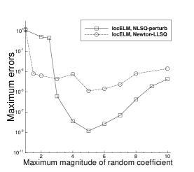
Figure 30: Effect of the random coefficients in local neural networks (nonlinear Helmholtz equation): the maximum error in the domain versus $R_{m}$, obtained with the NLSQ-perturb and Newton-LLSQ methods.

Figure 30 illustrates the effect of the random coefficients in the hidden layers of the local neural networks. In this group of tests we employ $N_{e}=4$ sub-domains, $Q=100$ uniform collocation points per sub-domain, $200$ training parameters per sub-domain, and a single hidden layer in the local neural networks. As discussed before, the weight/bias coefficients in the hidden layer of each local neural network are set to uniform random values generated on $[-R_{m},R_{m}]$. In these tests, we vary $R_{m}$ systematically and study its effect. Figure 30 shows the maximum error in the overall domain as a function of $R_{m}$, obtained with the NLSQ-perturb and the Newton-LLSQ methods. The error exhibits a behavior similar to what has been observed with the linear problems. The methods have a better accuracy with a range of moderate $R_{m}$ values, and the results are less accurate with very large or very small $R_{m}$ values. We again observe that the NLSQ-perturb result is significantly more accurate than that of Newton-LLSQ, except for a range of small $R_{m}$ values.

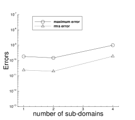
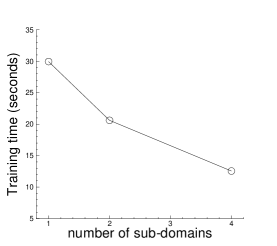
(a) (b)

Figure 31: Effect of the number of sub-domains, with fixed total degrees of freedom in the domain (nonlinear Helmholtz equation): (a) the maximum and rms errors in the domain, and (b) the training time, as a function of the number of sub-domains in the locELM simulation with NLSQ-perturb.

In Figure 31 we study the effect of the number of sub-domains on the simulation accuracy and the computational cost, while the total degrees of freedom in the domain are fixed. In these tests we vary the number of uniform sub-domains ($N_{e}$). We choose the number of uniform collocation points per sub-domain ($Q$) and the training parameters per sub-domain ($M$) such that the total number of collocation points in the domain is fixed at $N_{e}Q=400$ and the total number of training parameters in the domain is fixed at $N_{e}M=800$. We have tested three cases, corresponding to $N_{e}=1$, $2$ and $4$. As in the previous sections, the case with one sub-domain ($N_{e}=1$) corresponds to use of a global ELM. Figure 31(a) shows the maximum and rms errors in the overall domain as a function of the number of sub-domains. Figure 31(b) shows the corresponding training time versus the number of sub-domains. These results are obtained with the NLSQ-perturb method. We have employed $R_{m}=20.0$ when generating the random coefficients with one sub-domain ($N_{e}=1$), $R_{m}=10.0$ with two sub-domains ($N_{e}=10.0$) and $R_{m}=4.5$ with four sub-domains ($N_{e}=4.5$). These $R_{m}$ values approximately reside in the optimal range of $R_{m}$ values for these cases. One can observe that the numerical errors obtained with different number of sub-domains are comparable, with the errors obtained on four sub-domains a little worse than those of the other cases. On the other hand, the network training time decreases significantly with increasing number of sub-domains.

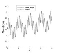
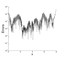
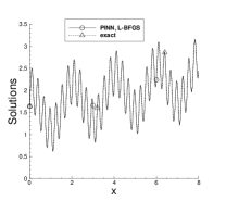
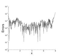
(a) (b) (c) (d)

Figure 32: Nonlinear Helmholtz equation: Distributions of the solutions (a,c) and their absolute errors (b,d) computed using PINN RaissiPK2019 with the Adam optimizer (a,b) and the L-BFGS optimizer (c,d). These can be compared with those in Figure 26 computed using locELM.

We next compare the current locELM method with the PINN method RaissiPK2019 for solving the nonlinear Helmholtz equation. Figure 32 shows distributions of the PINN solutions and their absolute errors against the exact solution given in equation (41), computed using the Adam optimizer (Figures 32(a,b)) and the L-BFGS optimizer (Figures 32(c,d)). With the Adam optimizer, the neural network consists of $7$ hidden layers, with a width of $50$ nodes in each layer and the $\tanh$ activation function, in addition to the input layer of one node (representing $x$) and the output layer of one node (representing the solution $u$). The network has been trained on the input data of $400$ uniform collocation points for $45,000$ epochs, with the learning rate gradually decreasing from $0.001$ at the beginning to $5\times 10^{-6}$ at the end of the training. With the L-BFGS optimizer, the neural network consists of $4$ hidden layers, with a width of $50$ nodes in each layer and the $\tanh$ activation function, apart from the input layer of one node and the output layer of one node. The network has been trained on the input data of $400$ uniform collocation points in the domain for $22,000$ L-BFGS iterations. The results indicate that the PINN method has captured the solution quite accurately, with the errors on the order $10^{-5}\sim 10^{-3}$ with the Adam optimizer and on the order $10^{-5}\sim 10^{-4}$ with the L-BFGS optimizer. Comparing the PINN results in this figure and the locELM results in Figure 26, we can observe that the locELM method is considerably more accurate than PINN.

method	maximum error	rms error	epochs/iterations	training time (seconds)
PINN (Adam)	$4.56e-3$	$5.04e-4$	$45,000$	$578.2$
PINN (L-BFGS)	$1.69e-3$	$1.69e-4$	$22,000$	$806.4$
locELM (NLSQ-perturb)	$1.45e-9$	$2.34e-10$	$71$	$7.7$
locELM (Newton-LLSQ)	$1.28e-5$	$1.75e-6$	$5$	$2.7$

Table 6: Nonlinear Helmholtz equation: comparison between locELM and PINN in terms of the maximum/rms errors in the domain, the number of epochs or nonlinear iterations, and the network training time. The problem settings and simulation parameters correspond to those of Figures 26 and 32.

Table 6 provides further comparisons between locELM and PINN in terms of the accuracy and the computational cost. Here we have listed the maximum and rms errors in the domain, the number of epochs or nonlinear iterations in the training, and the network training time, associated with the PINN (with Adam/L-BFGS optimizers) simulations and the current locELM simulations. The problem settings and the simulation parameters here correspond to those in Figure 26 with locELM and those in Figure 32 with PINN. It is evident that the current locELM method is much more accurate than PINN. For example, the errors obtained using locELM/NLSQ-perturb are about six orders of magnitude smaller than those obtained by PINN/L-BFGS. The errors obtained by locELM/Newton-LLSQ are about two orders of magnitude smaller than those of PINN/L-BFGS. Furthermore, the current method is computationally much cheaper than PINN, with the training time approximately two orders of magnitude smaller (e.g. about $8$ seconds with locELM/NLSQ-perturb versus around $806$ seconds with PINN/L-BFGS).

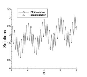
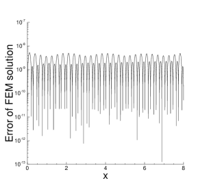
(a) (b)

Figure 33: Nonlinear Helmholtz equation: profiles of the solution (a) and its absolute error (b) computed using the finite element method (FEM) with $200,000$ uniform elements.

method	elements	sub-domains	$Q$	$M$	maximum	rms	wall-time
					error	error	(seconds)
locELM (NLSQ-perturb)	–	4	$100$	$200$	$1.45e-9$	$2.34e-10$	$7.7$
	–	4	$125$	$200$	$3.96e-11$	$7.02e-12$	$10.6$
FEM	$200,000$	–	–	–	$5.26e-9$	$1.37e-9$	$4.7$
	$400,000$	–	–	–	$1.31e-9$	$3.43e-10$	$8.8$
	$800,000$	–	–	–	$3.29e-10$	$8.57e-11$	$18.1$

Table 7: Nonlinear Helmholtz equation: comparison between locELM and FEM, in terms of the maximum/rms errors in the domain and the training/computation time. The problem settings correspond to those of Figures 26(a,b) and 33.

Let us now compare the current locELM method with the finite element method for solving the nonlinear Helmholtz equation. Figure 33 shows the profiles of the finite element solution and its absolute error against the analytic solution, computed on a mesh of $200,000$ uniform elements. The finite element method is again implemented using the FEniCS library in Python, and the nonlinear algebraic equation is solved using a Newton iteration. The FEM result is observed to be accurate, with an error level on the order $10^{-9}$. In Table 7 we compare the locELM method and the finite element method with regard to the accuracy and the computational cost. The table lists the maximum and rms errors in the domain and the wall time of the training or computation, obtained using locELM and FEM on several sets of parameters corresponding to different simulation resolutions. One can observe that locELM exhibits a comparable, and generally superior, performance to FEM. For example, the locELM case with $(Q,M)=(100,200)$ has a computational cost comparable to the FEM case with $400,000$ elements, and their error levels are also comparable. The locELM case with $(Q,M)=(125,200)$ has a lower cost ($\sim 10$ seconds) than the FEM case with $800,000$ elements ($\sim 18$ seconds), and also has considerably smaller errors, by an order of magnitude, than the latter.

3.4.2 Nonlinear Spring Equation

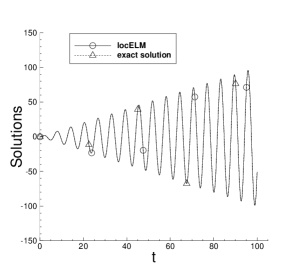
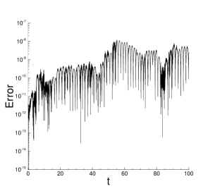
(a) (a)

Figure 34: Nonlinear spring: time histories of (a) the locELM solution and (b) its absolute error against the exact solution. $40$ uniform time blocks are used.

In the next example we test the locELM method using an initial value problem, the nonlinear spring. The goal here is to assess the performance of the locELM method together with the block time marching scheme, especially for long-time dynamic simulations.

Consider the temporal domain, $\Omega=[0,t_{f}]$, and the following initial value problem on this domain,

$$\frac{d^{2}u}{dt^{2}}+\omega^{2}u+\alpha\sin(u)=f(t),$$ (42a)

$$u(0)=u_{0},$$ (42b)

$$\left.\frac{du}{dt}\right|_{t=0}=v_{0},$$ (42c)

where $u(t)$ is the displacement, $f(t)$ is an imposed external force, $\omega$ and $\alpha$ are constant parameters, $u_{0}$ is the initial displacement, and $v_{0}$ is the initial velocity. The parameters in the above domain and problem specifications assume the following values in this subsection,

$$\omega=2,\quad\alpha=0.5,\quad t_{f}=100,\ \text{or}\ 15,\ \text{or}\ 2.5.$$

We choose the external force $f(t)$ such that the following function satisfies the equation (42a),

$$u(t)=t\sin(t).$$ (43)

We set the initial displacement and the initial velocity both to zero, i.e. $u_{0}=0$ and $v_{0}=0$. Under these settings, the initial value problem consisting of equations (42a)–(42c) has the solution given by (43).

We employ the locELM method and the block time marching scheme from Section 2.3.2 to solve this initial value problem. We partition the domain $[0,t_{f}]$ into $N_{b}$ uniform time blocks, and solve this initial value problem on each time block individually and successively. For the computation within each time block, we use a single sub-domain in the simulation, as the amount of data involved in is quite small because the function does not depend on space. We enforce the equations on $Q$ uniform collocation points within each time block. Accordingly, we employ a single neural network within each time block for this problem. The neural network consists of an input layer of one node (representing the time $t$), a single hidden layer with a width of $M$ nodes and the $\tanh$ activation function, and an output layer of one node (representing the solution $u$). The output layer is assumed to be linear (no activation function) and contains no bias. As in previous sections, we incorporate an affine mapping operation right behind the input layer to normalize the input $t$ data to the interval $[-1,1]$ for each time block. The weight and bias coefficients in the hidden layer of the neural network are pre-set to uniform random values generated on the interval $[-R_{m},R_{m}]$. A fixed seed value $1234$ is used for the random number generator. We employ the NLSQ-perturb method from Section 2.3.1 for computing the resultant nonlinear algebraic problem. The initial guess of the solution is set to zero. In the event the random perturbation is triggered, we employ $\delta=1.0$ and $\xi_{2}=1$ (see Algorithm 1 and Remark 2.7) for generating the random perturbations in the tests of this subsection.

The locELM simulation parameters include the number of time blocks $N_{b}$, the number of collocation points per time block $Q$, the number of training parameters per time block $M$ (i.e. the number of nodes in the hidden layer of the neural network), and the maximum magnitude of the random coefficients $R_{m}$.

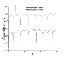
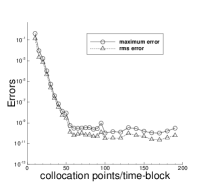
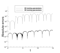
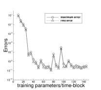
(a) (b) (c) (d)

Figure 35: Nonlinear spring: (a) Error histories obtained with $20$ and $40$ collocation points per time block. (b) The maximum/rms errors in the domain versus the number of collocation points per time block. In (a) and (b), the number of training parameters per time block is fixed at $100$. (c) Error histories obtained with $20$ and $30$ training parameters per time block. (d) The maximum/rms errors versus the number of training parameters per time block. In (c) and (d) the number of the collocation points per time block is fixed at $60$.

Figure 34 shows the time histories of the displacement and its absolute error obtained using locELM in a fairly long-time simulation. The time history of the exact solution given by (43) has also been shown in Figure 34(a) for comparison. In this test the domain size is set to $t_{f}=100$. We have employed $N_{b}=40$ uniform time blocks within the domain, $Q=60$ uniform collocation points per time block, $M=100$ training parameters per time block, and $R_{m}=5.0$ when generating the random weight/bias coefficients for the hidden layer of the neural network. It is evident that the current locELM method has captured the solution very accurately, with the maximum level of the absolute error on the order $10^{-8}$ over the entire domain.

Figure 35 illustrates the effect of the number of degrees of freedom (collocation points, training parameters) on the simulation accuracy. In this group of tests the temporal domain size is set to $t_{f}=15$, and we employ $N_{b}=6$ time blocks within the domain. Figure 35(a) shows the absolute-error histories of the locELM solution against the exact solution, obtained using $20$ and $40$ collocation points per time block. Figure 35(b) shows the maximum and rms errors in the overall domain obtained with different numbers of collocation points in the locELM simulation. The number of training parameters per time block is fixed at $M=100$ with the tests in these two plots. The errors can be observed to decrease exponentially as the number of collocation points per time block increases (when below around $60$), and then become stagnant as the number of collocation points increases further. Figure 35(c) shows time histories of the absolute errors corresponding to $20$ and $40$ training parameters per time block. Figure 35(d) shows the maximum/rms errors in the overall domain, obtained with different numbers of training parameters per time block. In the tests of these two plots, the number of collocation points per time block has been fixed at $Q=60$. The convergence with respect to the training parameters is not as regular as that for the collocation points. Nonetheless, one can see that the errors approximately decrease exponentially with increasing number of training parameters (when below $50$), and then they essentially stagnate as the number of training parameters increases further.

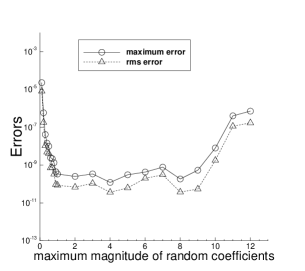
Figure 36: Nonlinear spring: The maximum and rms errors in the overall domain as a function of $R_{m}$, the maximum magnitude of the random coefficients.

Figure 36 demonstrates the effect of $R_{m}$, the maximum magnitude of the random coefficients, on the simulation accuracy. In this set of tests, the temporal domain size is $t_{f}=15$. We have employed $N_{b}=6$ uniform time blocks in the domain, $Q=60$ uniform collocation points in each time block, and $M=100$ training parameters per time block. The value of $R_{m}$ is varied systematically in the tests. In this figure we plot the maximum and rms errors in the overall domain corresponding to different $R_{m}$ values. The characteristics observed here are consistent with those from previous subsections. The locELM method has a better accuracy with $R_{m}$ in a range of moderate values, and in this case approximately $R_{m}=1\sim 9$. The results are less accurate if $R_{m}$ is very large or very small.

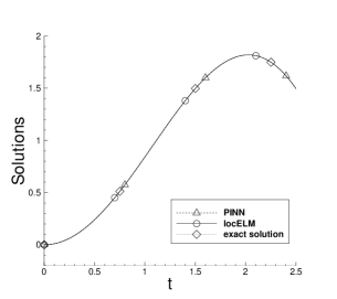
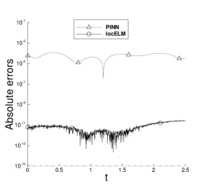
(a) (a)

Figure 37: Comparison between locELM and PINN (nonlinear spring): Time histories of (a) the solutions and (b) their absolute errors, computed using PINN RaissiPK2019 with the Adam optimizer and using locELM with the NLSQ-perturb method. The temporal domain size is $t_{f}=2.5$.

method	maximum error	rms error	epochs/iterations	training time (seconds)
PINN (Adam)	$1.21e-4$	$6.71e-5$	$20,000$	$26.3$
locELM (NLSQ-perturb)	$2.82e-11$	$1.12e-11$	$48$	$0.34$

Table 8: Nonlinear spring: Comparison between locELM and PINN in terms of the maximum/rms errors in the domain, the number of epochs or nonlinear iterations in the training, and the network training time. The problem settings and the simulation parameters correspond to those of Figure 37.

Let us next compare the current locELM method with PINN RaissiPK2019 for solving the nonlinear spring equation. Figure 37 shows a comparison of the time histories of the solutions and their absolute errors obtained using PINN with the Adam optimizer and using the current locELM method with NLSQ-perturb. In this group of tests, the temporal domain size is set to $t_{f}=2.5$. In the PINN simulation, the neural network consists of an input layer of one node (representing $t$), three hidden layers with a width of $10$ nodes and the $\tanh$ activation function in each layer, and an output layer of one node (representing the solution $u$). The input data consists of $500$ uniform collocation points from the domain $[0,t_{f}]$. The neural network has been trained using the Adam optimizer for $20,000$ epochs, with the learning rate decreasing from $0.01$ at the beginning to $1e-5$ at the end of the training. In the locELM simulation, we employ a single time block ($N_{b}=1$) in the domain, $Q=60$ uniform collocation points within the time block, $M=100$ training parameters in the time block, a single hidden layer in the neural network, and $R_{m}=5.0$ for generating the random weight/bias coefficients. Figure 37 demonstrates that both PINN and locELM have captured the solution accurately, but the error of the locELM result is considerably smaller than that of PINN.

Table 8 provides a further comparison between locELM and PINN in terms of their accuracy and computational cost. The problem settings and the simulation parameters here correspond to those of Figure 37. We have listed the maximum and rms errors of the PINN and locELM results in the overall domain, the number of epochs or nonlinear iterations in the training, and the network training time. The data demonstrate that the current locELM method is much more accurate, by six orders of magnitude, than PINN, and the network training time of locELM is much smaller, by nearly two orders of magnitude, than that of PINN.

3.4.3 Viscous Burger’s Equation

In this subsection we further test the locELM method using the viscous Burger’s equation. Consider the spatial-temporal domain $\Omega=\{(x,t)\ |\ x\in[a,b],\ t\in[0,t_{f}]\}$, and the following initial/boundary value problem with the Burger’s equation,

$$\frac{\partial u}{\partial t}+u\frac{\partial u}{\partial x}=\nu\frac{\partial^{2}u}{\partial x^{2}}+f(x,t),$$ (44a)

$$u(a,t)=g_{1}(t),$$ (44b)

$$u(b,t)=g_{2}(t),$$ (44c)

$$u(x,0)=h(x),$$ (44d)

where $u(x,t)$ is the solution to be solved for, the constant $\nu$ denotes the viscosity, $f(x,t)$ is a prescribed source term, $g_{1}(t)$ and $g_{2}(t)$ denote the boundary distributions, and $h(x)$ is the initial distribution. We employ the following values for the constant parameters,

$$\nu=0.01,\quad a=0,\quad b=5,\quad t_{f}=10,\ \text{or}\ 2.5,\ \text{or}\ 0.25.$$

We choose the source term $f(x,t)$ and the boundary/initial distributions ($g_{1}$, $g_{2}$ and $h$) such that the following function

$$\begin{split}u(x,t)=&\left(1+\frac{x}{10}\right)\left(1+\frac{t}{10}\right)\left[2\cos\left(\pi x+\frac{2\pi}{5}\right)+\frac{3}{2}\cos\left(2\pi x-\frac{3\pi}{5}\right)\right]\left[2\cos\left(\pi t+\frac{2\pi}{5}\right)\right.\\ &\left.+\frac{3}{2}\cos\left(2\pi t-\frac{3\pi}{5}\right)\right]\end{split}$$ (45)

satisfies this initial/boundary value problem.

We employ the method presented in Section 2.3.2 with block time marching to solve this problem, by restricting the method to one spatial dimension. The spatial-temporal domain $\Omega$ is partitioned into $N_{b}$ uniform blocks in time, and each time block is computed separately and successively. Within each time block, we further partition its spatial-temporal domain into $N_{x}$ uniform sub-domains in $x$ and $N_{t}$ uniform sub-domains in time, resulting in $N_{e}=N_{x}N_{t}$ uniform sub-domains per time block. $C^{1}$ continuity is imposed on the sub-domain boundaries in the $x$ direction, and $C^{0}$ continuity is imposed on the sub-domain boundaries in the temporal direction. Within each sub-domain we employ a total of $Q=Q_{x}Q_{t}$ uniform collocation points, with $Q_{x}$ uniform collocation points in the $x$ direction and $Q_{t}$ uniform collocation points in time.

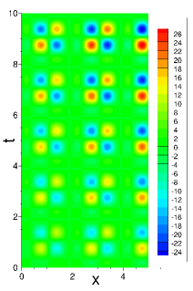
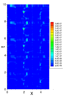
(a) (b)

Figure 38: Burgers equation: distributions of (a) the solution, and (b) its absolute error in the spatial-temporal plane, computed using the current locELM (NLSQ-perturb) method.

We employ a local neural network for each sub-domain, leading to a total of $N_{e}$ local neural networks in the simulations. Each local neural network consists of an input layer of two nodes, representing the $x$ and $t$, a single hidden layer with a width of $M$ nodes and the $\tanh$ activation function, and an output layer of a single node, representing the field solution $u$. The output layer has no bias and no activation function. Additionally, an affine mapping operation is incorporated into the network right behind the input layer to normalize the input $x$ and $t$ data to the interval $[-1,1]\times[-1,1]$ for each sub-domain. The weight/bias coefficients in the hidden layer of the local neural networks are pre-set to uniform random values generated on the interval $[-R_{m},R_{m}]$, and are fixed during the simulation. A fixed seed value $22$ is used for the Tensorflow random number generator for all the tests in this sub-section.

We employ the NLSQ-perturb method from Section 2.3.1 for computing the resultant nonlinear algebraic problem in the majority of tests presented below. The results computed using Newton-LLSQ are also provided for comparison in some cases. The initial guess of the solution is set to zero. With the NLSQ-perturb method, we employ $\delta=0.5$ and $\xi_{2}=0$ (see Algorithm 1 and Remark 2.7) for generating the random perturbations in the following tests.

The locELM simulation parameters include the number of time blocks ($N_{b}$), the number of sub-domains per time block ($N_{e}$, $N_{x}$, $N_{t}$), the number of collocation points per sub-domain ($Q$, $Q_{x}$, $Q_{t}$), the number of training parameters per sub-domain ($M$), and the maximum magnitude of the random coefficients ($R_{m}$).

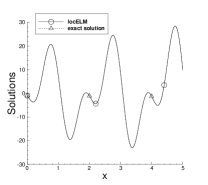
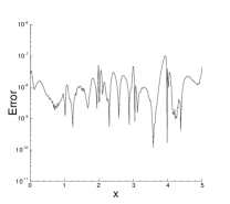
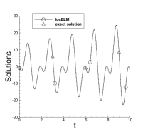
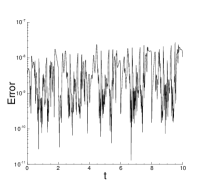
(a) (b) (c) (d)

Figure 39: Burger’s equation: Profiles of the locELM (NLSQ-perturb) solution (a) and its absolute error (b) at $t=8.75$. Time histories of the locELM (NLSQ-perturb) solution (c) and its absolute error (d) at the point $x=2.75$. The settings and simulation parameters correspond to those of Figure 38.

Figure 38 shows distributions of the solution and its absolute error in the spatial-temporal plane, computed using the current locELM method (with NLSQ-perturb). Here the temporal domain size is set to be $t_{f}=10$, and $40$ uniform time blocks ($N_{b}=40$) are used in the spatial-temporal domain. We have employed $N_{e}=5$ uniform sub-domains with $N_{x}=5$ and $N_{t}=1$ within each time block, $Q=20\times 20$ uniform collocation points per sub-domain ($Q_{x}=Q_{t}=20$), $M=200$ training parameters per sub-domain, and $R_{m}=0.75$ when generating the random coefficients. The current method has captured the solution accurately, with the absolute error on the order $10^{-8}\sim 10^{-7}$ in the overall domain.

Figure 39 further examines the accuracy of the locELM solution. The problem settings and the simulation parameters here correspond to those of Figure 38. Figures 39(a) and (b) depict the profiles of the locELM (NLSQ-perturb) solution and its absolute error at the time $t=8.75$. The exact solution profile at this time instant is also shown in Figure 39(a). The locELM solution profile exactly overlaps with that of the exact solution, and the absolute error is around the level $10^{-10}\sim 10^{-7}$. Figures 39(c) and (d) show the time histories of the locELM (NLSQ-perturb) solution and its absolute error at the point $x=2.75$. The time history of the exact solution at this point is also shown in Figure 39(c). The simulated signal overlaps with that of the exact signal, and the absolute error can be observed to fluctuate around the level $10^{-10}\sim 10^{-8}$.

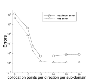
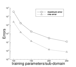
(a) (b)

Figure 40: Effect of the degrees of freedom on the accuracy (Burger’s equation): the maximum and rms errors in the domain as a function of (a) the number of collocation points in each direction per sub-domain, and (b) the number of training parameters per sub-domain.

Figure 40 demonstrates the effect of the degrees of freedom on the simulation accuracy. In this group of tests the temporal domain size is set to $t_{f}=2.5$. We have employed $N_{b}=10$ uniform time blocks in the overall spatial-temporal domain, $N_{e}=5$ uniform sub-domains per time block (with $N_{x}=5$ and $N_{t}=1$), and $R_{m}=0.5$ when generating random coefficients for the hidden layers of the local neural networks. First, we fix the number of training parameters per sub-domain to $M=200$, and vary the number of (uniform) collocation points per sub-domain systematically while maintaining $Q_{x}=Q_{t}$. Figure 40(a) shows the maximum and rms errors in the overall domain versus the number of collocation points in each direction per sub-domain. It is observed that the errors decrease essentially exponentially with increasing number of collocation points per direction (when below around $Q_{x}=Q_{t}=15$). Then the errors stagnate as the number of collocation points per direction increases beyond $15$, due to the saturation associated with the fixed number of training parameters in the test. Then, we fix the number of uniform collocation points to $Q=20\times 20$ per sub-domain, and vary the number of training parameters per sub-domain systematically in a range of values. Figure 40(b) shows the resultant maximum/rms errors in the overall domain versus the number of training parameters per sub-domain. As the number of training parameters per sub-domain increases, the locELM errors can be observed to decrease substantially.

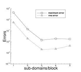
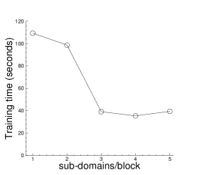
(a) (b)

Figure 41: Effect of the number of sub-domains, with fixed total degrees of freedom in the domain (Burger’s equation): (a) the maximum and rms errors in the domain, and (b) the training time, as a function of the number of uniform sub-domains per time block. Temporal domain size is $t_{f}=0.25$, and a single time block is used in the spatial-temporal domain.

Figure 41 demonstrates the effect of the number of sub-domains, with the total number of degrees of freedom in the domain (approximately) fixed. In this group of tests, the temporal domain size is set to $t_{f}=0.25$, and we employ a single time block in the spatial-temporal domain. We employ uniform sub-domains, and vary the number of sub-domains within the time block systematically between $N_{e}=1$ and $N_{e}=5$ (with fixed $N_{t}=1$ and various $N_{x}$). The number of (uniform) collocation points per sub-domain and the number of training parameters per sub-domain are both varied, but the total number of collocation points and the total number of training parameters in the time block are fixed approximately at $N_{e}Q\approx 2000$ and $N_{e}M\approx 1000$, respectively. More specifically, we employ $Q=45\times 45$ collocation points/sub-domain and $M=1000$ training parameters/sub-domain with $N_{e}=1$ sub-domain within the time block, $Q=32\times 32$ collocation points/sub-domain and $M=500$ training parameters/sub-domain with $N_{e}=2$ sub-domains, $Q=26\times 26$ collocation points/sub-domain and $M=333$ training parameters/sub-domain with $N_{e}=3$ sub-domains, $Q=22\times 22$ collocation points/sub-domain and $M=250$ training parameters/sub-domain with $N_{e}=4$ sub-domains, and $Q=20\times 20$ collocation points/sub-domain and $M=200$ training parameters/sub-domain with $N_{e}=5$ sub-domains within the time block. When generating the random weight/bias coefficients, we have employed $R_{m}=2.0$ with $N_{e}=1$ sub-domain in the time block, $R_{m}=1.0$ with $N_{e}=2$ and $3$ sub-domains, and $R_{m}=0.75$ with $N_{e}=4$ and $5$ sub-domains within the time block. These values are approximately in the optimal range of $R_{m}$ values for these cases. Figure 41(a) shows the maximum and rms errors of the locELM (NLSQ-perturb) solution in the domain as a function of the number of sub-domains within the time block. We observe that the errors decrease quite significantly, by nearly two orders of magnitude, as the number of sub-domains increases from $N_{e}=1$ to $N_{e}=3$. The errors remain approximately at the same level with three and more sub-domains. Note that the case with one sub-domain corresponds to the global ELM computation. These results indicate that the local ELM simulation with multiple sub-domains appears to achieve a better accuracy than the global ELM simulation for this problem. Figure 41(b) shows the training time of the neural network as a function of the number of sub-domains. The training time has been reduced substantially as the number of sub-domains increases from one to three sub-domains (from around $110$ seconds to about $40$ seconds), and it remains approximately the same with three and more sub-domains. These results show that, compared with the global ELM, the use of domain decomposition and multiple sub-domains in locELM can significantly reduce the computational cost for the Burger’s equation. This is consistent with the observations with the other problems in previous sections.

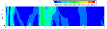
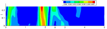
(a) (b)

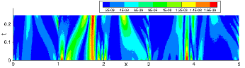
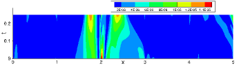
(c) (d)

Figure 42: Comparison between locELM and DGM (Burger’s equation): distributions of the absolute errors computed using DGM with the Adam optimizer (a) and L-BFGS optimizer (b), and using locELM with NLSQ-perturb (c) and with Newton-LLSQ (d).

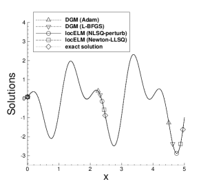
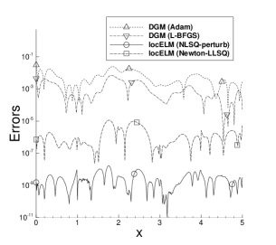
(a) (b)

Figure 43: Burger’s equation: Profiles of (a) the solutions and (b) their absolute errors at $t=0.2$ computed using DGM and locELM. The settings and simulation parameters correspond to those of Figure 42.

method	maximum error	rms error	epochs/iterations	training time (seconds)
DGM (Adam)	$4.57e-2$	$5.76e-3$	$128,000$	$1797.8$
DGM (L-BFGS)	$7.50e-3$	$1.55e-3$	$28,000$	$1813.5$
locELM (NLSQ-perturb)	$1.85e-8$	$4.44e-9$	$27$	$27.6$
locELM (Newton-LLSQ)	$1.62e-5$	$3.11e-6$	$15$	$9.1$

Table 9: Burger’s equation: comparison between locELM and DGM in terms of the maximum/rms errors in the domain, the number of epochs or nonlinear iterations, and the network training time. The problem settings and simulation parameters correspond to those of Figure 42.

We next compare the current locELM method with the deep Galerkin method (DGM) for the Burger’s equation. Figure 42 is a comparison of distributions of the solutions (left column) and their absolute errors (right column) in the spatial-temporal plane, obtained using DGM with the Adam and L-BFGS optimizers (top two rows) and using the current locELM method with NLSQ-perturb and Newton-LLSQ (bottom two rows). In these tests the temporal domain size is set to $t_{f}=0.25$. For DGM, the neural network consists of an input layer of two nodes (representing $x$ and $t$), $5$ hidden layers with a width of $40$ nodes in each layer and the $\tanh$ activation function, and an output layer of a single node (representing $u$) with no bias and no activation function. When computing the loss function, the spatial-temporal domain has been divided into $10$ uniform sub-domains along the $x$ direction, and we have used $10\times 10$ Gauss-Lobatto-Legendre quadrature points in each sub-domain for computing the residual norms. With the Adam optimizer, the neural network has been trained for $128,000$ epochs, with the learning rate gradually decreasing from $0.001$ at the beginning to $10^{-5}$ at the end of the training. With the L-BFGS optimizer, the neural network has been trained for $28,000$ iterations. For the current locELM method, we have employed a single time block in the spatial-temporal domain and $N_{e}=5$ uniform sub-domains along the $x$ direction within this time block. With NLSQ-perturb, we have employed $Q=20\times 20$ uniform collocation points per sub-domain, $M=200$ training parameters per sub-domain, and $R_{m}=0.75$ when generating the random coefficients. With Newton-LLSQ, we have employed $Q=20\times 20$ uniform collocation points per sub-domain, $M=150$ training parameters per sub-domain, and $R_{m}=1.0$ when generating the random coefficients. The results in Figure 42 indicate that the current locELM method is considerably more accurate than DGM for the Burger’s equation. The errors of the current method is generally several orders of magnitude smaller than those of DGM. The locELM method with NLSQ-perturb provides the best accuracy, with the errors on the order $10^{-9}\sim 10^{-8}$. Then it is the locELM method with Newton-LLSQ, with the errors on the level $10^{-6}\sim 10^{-5}$. In contrast, the errors of the DGM with Adam and L-BFGS are generally on the levels $10^{-3}\sim 10^{-2}$ and $10^{-3}$, respectively.

Figure 43 compares the profiles of the DGM and locELM solutions (plot (a)) and their errors (plot (b)) at the time instant $t=0.2$. The profile of the exact solution at this instant is also included in Figure 43(a) for comparison. The problem settings and the simulation parameters here correspond to those of Figure 42. The solution profiles from DGM and locELM simulations are in good agreement with that of the exact solution. The error profiles, on the other hand, reveal disperate accuracies in the results obtained using these methods. They confirm the ordering of these methods, from the most to the least accurate, to be locELM/NLSQ-perturb, locELM/Newton-LLSQ, DGM/L-BFGS, and DGM/Adam.

Table 9 provides a further comparison between locELM and DGM for the Burger’s equation, in terms of their accuracy and computational cost. We have listed the maximum and rms errors in the overall spatial-temporal domain, the number of epochs or nonlinear iterations in the training, and the training time of the neural network corresponding to DGM with the Adam/L-BFGS optimizers and the current locELM method with NLSQ-perturb and Newton-LLSQ. The observations here are consistent with those of previous sections. The locELM method is orders of magnitude more accurate than DGM (e.g. $10^{-8}$ with locELM/NLSQ-perturb versus $10^{-3}$ with DGM/L-BFGS), and its training time is orders of magnitude smaller than that of DGM (e.g. around $28$ seconds with locELM/NLSQ-perturb versus around $1800$ seconds with DGM/L-BFGS).

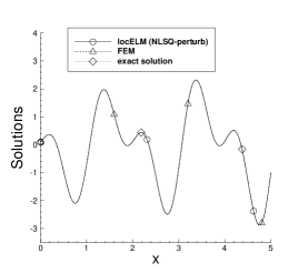
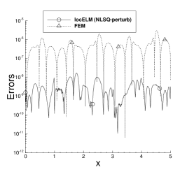
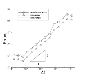
(a) (b) (c)

Figure 44: Comparison between locELM and FEM (Burger’s equation): Profiles of (a) the solutions and (b) their absolute errors at $t=0.2$, computed using locELM (with NLSQ-perturb) and using FEM. (c) The maximum and rms errors at $t=0.25$ versus $\Delta t$ computed using FEM (with a mesh of $10,000$ uniform elements), showing its second-order convergence rate in time.

method	elements	$\Delta t$	sub-	$Q$	$M$	maximum	rms	wall-time
			domains			error	error	(seconds)
locELM	–	–	$5$	$15\times 15$	$150$	$2.10e-6$	$4.35e-7$	$14.7$
(NLSQ-perturb)	–	–	$5$	$20\times 20$	$200$	$1.85e-8$	$4.44e-9$	$27.6$
locELM	–	–	$5$	$15\times 15$	$150$	$1.25e-5$	$2.71e-6$	$6.8$
(Newton-LLSQ)	–	–	$5$	$20\times 20$	$150$	$1.62e-5$	$3.11e-6$	$9.1$
FEM	2000	$0.001$	–	–	–	$2.64e-5$	$5.15e-6$	$12.5$
	2000	$0.0005$	–	–	–	$3.07e-5$	$5.76e-6$	$25.4$
	5000	$0.001$	–	–	–	$1.89e-5$	$1.74e-6$	$26.0$
	5000	$0.0005$	–	–	–	$4.13e-6$	$7.90e-7$	$50.8$
	10000	$0.001$	–	–	–	$2.22e-5$	$1.99e-6$	$47.7$
	10000	$0.0005$	–	–	–	$4.74e-6$	$4.36e-7$	$92.6$

Table 10: Burger’s equation: comparison between locELM and FEM in terms of the maximum/rms errors in the domain and the training/computation time. $Q$ and $M$ denote the number of collocation points per sub-domain and the number of training parameters per sub-domain, respectively.

Finally, we compare the current locELM method with the classical finite element method for solving the Burger’s equation. In the FEM simulation, we discretize the Burger’s equation (44a) in time using a semi-implicit scheme. We treat the nonlinear term explicitly and the viscous term implicitly, and discretize the time derivative by the second-order backward differentiation formula (BDF2). The method is again implemented using the FEniCS library in Python. Figures 44(a) and (b) show a comparison of the solution and error profiles at $t=0.2$ obtained using the current locELM (NLSQ-perturb) method and using the finite element method. Figure 44(c) shows the numerical errors at $t=0.25$ as a function of the time step size $\Delta t$ computed using the finite element method. In these simulations the temporal domain size is $t_{f}=0.25$. In Figures 44(a,b), the FEM simulation is conducted with $\Delta t=1.25e-4$ on a mesh of $10,000$ uniform elements, and the locELM simulation is conducted with a single time block in the domain and $N_{e}=5$ sub-domains in the time block, with $(Q,M)=(20\times 20,200)$ and $R_{m}=0.75$. In Figure 44(c), the simulations are performed with a fixed mesh of $10,000$ uniform elements. It can be observed that both locELM and FEM have produced accurate solutions, and that the FEM exhibits a second-order convergence rate in time before the error saturation when $\Delta t$ becomes very small.

Table 10 provides a comparison between locELM and FEM in terms of their accuracy and computational cost for the Burger’s equation. The temporal domain size is $t_{f}=0.25$ in these tests. We solve the problem using locELM and FEM on several sets of simulation parameters with different numerical resolutions. The maximum and rms errors in the spatial-temporal domain are computed, and we also record the training time of locELM and the computation time of FEM in these simulations. We list in this table the maximum and rms errors, as well as the training/computation time, corresponding to different simulation parameters for the locELM method with NLSQ-perturb and Newton-LLSQ and for the finite element method. A single time block has been used in the spatial-temporal domain for the locELM simulations, and we employ $R_{m}=0.75$ with locELM/NLSQ-perturb and $R_{m}=1.0$ with locELM/Newton-LLSQ for generating the random coefficients. It is observed that the current locELM method with both NLSQ-perturb and Newton-LLSQ shows a superior performance to the FEM. For example, the two cases with locELM/Newton-LLSQ have numerical errors comparable to the FEM cases with $2000$ elements (for both $\Delta t$), $5000$ elements ($\Delta t=0.001$) and $10000$ elements ($\Delta t=0.001$), but the computational cost of locELM/Newton-LLSQ is notably smaller than the cost of these FEM cases. The locELM/NLSQ-perturb case with $(Q,M)=(15\times 15,150)$ has numerical errors comparable to the FEM cases with $5000$ elements ($\Delta t=0.0005$) and $10000$ elements ($\Delta t=0.0005$), but the computational cost of this locELM/NLSQ-perturb case is only a fraction of those of these two FEM cases. The locELM/NLSQ-perturb case with $(Q,M)=(20\times 20,200)$ has a computational cost comparable to the FEM cases with $2000$ elements ($\Delta t=0.0005$) and $5000$ elements ($\Delta t=0.001$), but the errors of this locELM/NLSQ-perturb case are nearly three orders of magnitude smaller than those of these two FEM cases.

4 Concluding Remarks

In this paper we have developed an efficient method based on domain decomposition and local extreme learning machines (termed locELM) for solving linear and nonlinear partial differential equations. The problem domain is partitioned into sub-domains, and the field solution on each sub-domain is represented by a local shallow feed-forward neural network, consisting of a small number (one or more) of hidden layers. $C^{k}$ continuity, with $k$ determined by the order of the PDE, is imposed on the sub-domain boundaries. The overall neural network constitutes a multi-input multi-output model consisting of the local neural networks. The weight/bias coefficients in the hidden layers of all the local neural networks are pre-set to random values, and are fixed throughout the computation. The training parameters are composed of the weight coefficients in the output layers of the local neural networks.

We employ a set of collocation points within each sub-domain, the collection of which constitutes the input data to the neural network. The PDE is enforced on the collocation points in each sub-domain, and the derivatives involved therein are computed by auto-differentiation. The boundary and initial conditions are enforced on those collocation points that reside on the spatial and temporal boundaries of the spatial-temporal domain. The $C^{k}$ continuity conditions are enforced on those collocation points that reside on the corresponding sub-domain boundaries. These operations result in a system of linear or nonlinear algebraic equations about the set of training parameters. We seek a least squares solution to this system, and compute the solution by a linear least squares routine or a nonlinear least squares method. Training the overall neural network consists of the linear or nonlinear least squares computations. It should be noted that this training method is different from the back propagation-type algorithms.

For longer-time simulations of time-dependent PDEs, we have developed a block time-marching scheme together with the locELM method. The spatial-temporal domain is first divided into a number of windows in time, referred to as time blocks, and we solve the PDE on each time block separately and successively. The locELM method is then applied to the spatial-temporal domain of each time block to find the solution, as discussed in foregoing paragraphs. We observe that when the temporal dimension of the domain is large, if without block time marching, the neural network can become very difficult to train. On the other hand, with block time marching and using a moderate time block size, the problem is more manageable and much easier to solve. Block time marching requires re-training of the overall neural network on different time blocks, and so all network trainings become online operations. This is feasible with the current locELM method thanks to its high accuracy and low computational cost. We have demonstrated the capability of the current method for long-time dynamic simulations with the advection equation.

We have performed extensive numerical experiments to test the locELM method, and compared extensively the locELM method with DGM, PINN, global ELM, and the classical finite element method (FEM). We have the following observations:

• The locELM method exhibits a clear sense of convergence with increasing number of degrees of freedom. Its errors typically decrease exponentially or nearly exponentially as the number of sub-domains, or the number of collocation points/sub-domain, or the number of training parameters/sub-domain increases.

• The random weight/bias coefficients in the hidden layers of local neural networks influence the simulation accuracy. In the current work, these weight/bias coefficients are set to uniform random values generated on $[-R_{m},R_{m}]$. The simulation accuracy tends to decrease with very large or very small $R_{m}$ values. Higher accuracy is generally associated with a range of moderate $R_{m}$ values. This range of optimal $R_{m}$ values tends to expand when the number of collocation points/sub-domain or the number of training parameters/sub-domain increases.

• The network training time generally increases linearly (or super-linearly for some problems) with respect to the number of sub-domains in the simulation. It also tends to increase with respect to the number of collocation points/sub-domain and to the number of training parameters/sub-domain, but the relation is not quite regular.

• When the total degrees of freedom (total collocation points, total training parameters) in the system are fixed, increasing the number of sub-domains in the simulation, hence with the number of collocation points/training parameters per sub-domain correspondingly reduced, generally leads to simulation results with comparable accuracy, but it can dramatically reduce the network training time. Compared with global ELM, which corresponds to the locELM configuration with a single sub-domain, the use of domain decomposition and multiple sub-domains in locELM can significantly reduce the network training time, and produce results with comparable accuracy.

• The current locELM method shows a clear superiority to DGM and PINN, which are some of the commonly-used DNN-based PDE solvers, in terms of both accuracy and computational cost. The numerical errors and the network training time of locELM are considerably smaller, typically by orders of magnitude, than those of DGM and PINN.

• The current locELM method exhibits a computational performance that is comparable, and oftentimes superior, to the classical finite element method. With the same computational cost, the locELM errors are comparable to, and oftentimes considerably smaller than, the FEM errors. To achieve the same accuracy, the training time of locELM is comparable to, and oftentimes markedly smaller than, the FEM computation time.

We would like to make some further comments with regard to $R_{m}$, the maximum magnitude of the random weight/bias coefficients in the hidden layers of the local neural networks. As discussed above, the simulation results have a better accuracy if $R_{m}$ falls into a range of moderate values for a given problem. Let us consider the following question: given a new problem (e.g. a new PDE), how do we know what this range is and how do we find this range of optimal $R_{m}$ values in practice? The approximate range of these optimal $R_{m}$ values can be estimated readily by preliminary numerical experiments. Here is the basic idea. Given a new problem, one can always add some source terms to the PDE or to the boundary/initial conditions, and then manufacture a solution to the given problem, with the augmented source terms. Then one can use the manufactured solution to evaluate the accuracy of a set of preliminary simulations by varying the $R_{m}$ systematically. This will provide a reasonable estimate for the range of optimal $R_{m}$ values. After that, one can conduct actual simulations of the given problem, without the added source term, by using an $R_{m}$ value from the estimated range.

Some further comments are also in order concerning the numerical tests with fixed total degrees of freedom in the domain, while the number of sub-domains is varied. Because the total degrees of freedom in the domain is fixed, the degrees of freedom (number of collocation points, number of training parameters) per sub-domain decrease as the number of sub-domains increases. One can anticipate that, when the number of sub-domains becomes sufficiently large, the number of degrees of freedom per sub-domain can become very small. This will be bound to adversely affect the simulation accuracy, because the solution is represented locally by these degrees of freedom on each sub-domain. Therefore, if the total degrees of freedom in the domain are fixed, when the number of sub-domains in domain decomposition increases beyond a certain point, the simulation accuracy will start to deteriorate. The afore-mentioned observation about comparable accuracy with increasing number of sub-domains, with fixed total degrees of freedom in the domain, is for the cases where the number of sub-domains is below that point.

Deep neural network based PDE solvers have stimulated a great deal of interest in the past few years, as it offers a new way to parameterize and represent unknown field functions. The computational performance of these DNN-based methods so far is promising, but less than satisfying. A survey of related literature indicates that the error of these PDE solvers is generally on, and rarely goes beyond, the level of $10^{-2}\sim 10^{-3}$. The accuracy of such levels may be deemed remarkable for other application areas such as image classification. For scientific computing, however, it is less than satisfactory, especially considering that the classical numerical methods can achieve the machine accuracy given sufficient mesh resolution and computation time. Perhaps because of such poor error levels, a sense of convergence with a certain rate is generally lacking with the DNN-based PDE solvers. For example, when the number of layers or the number of nodes within the layers or the number of training data points is varied systematically, one can hardly observe an improvement or a systematic improvement in the accuracy of the obtained results. Another factor concerns the computational cost. The computational cost of DNN-based PDE solvers is very high, as demonstrated here and also by other works in the literature. The neural network of these solvers takes a considerable amount of time to train, in order to reach a reasonable level of accuracy. Because of their poorer accuracy and large computational cost, there seems to be a general sense that these DNN-based PDE solvers cannot compete with classical numerical methods, except perhaps in certain problems such as high-dimensional PDEs which can be challenging to classical methods due to the so-called curse of dimensionality.

The current locELM method developed herein, also based on neural networks, exhibits completely different performance characteristics. The current method demonstrates a clear sense of convergence, often with an exponential convergence rate, with respect to the degrees of freedom in the system such as the number of training parameters and the number of collocation points. As demonstrated by ample examples, the accuracy of the current method is far superior to, typically by orders of magnitude, and its computational cost is far less, also often by orders of magnitude, than those of the deep Galerkin method and the Physics-Informed Neural Network, which are both commonly-used DNN-based PDE solvers.

As demonstrated by ample examples in this paper, the computational performance of the current locELM method is on par with, and oftentimes exceeds, that of the classical finite element method. The importance of this point cannot be overstated. To the best of the authors’ knowledge, this seems to be the first time when a neural network-based method delivers the same performance as, or a better performance than, a traditional numerical method for the commonly-encountered computational problems in low dimensions. The current method demonstrates the great potential, and perhaps points toward a path forward, for neural network-based methods to be truly competitive, and excel, in computational science and engineering simulations.

5 Appendix. Additional Numerical Tests

5.1 Two-Dimensional Helmholtz Equation

We consider the boundary value problem with the two-dimensional (2D) Helmholtz equation on a rectangular domain, $\Omega=[a_{1},b_{1}]\times[a_{2},b_{2}]$, as follows,

$$\frac{\partial^{2}u}{\partial x^{2}}+\frac{\partial^{2}u}{\partial y^{2}}-\lambda u=f(x,y),$$ (46a)

$$u(a_{1},y)=h_{1}(y),$$ (46b)

$$u(b_{1},y)=h_{2}(y),$$ (46c)

$$u(x,a_{2})=h_{3}(x),$$ (46d)

$$u(x,b_{2})=h_{4}(x),$$ (46e)

where $u(x,y)$ is the field function to be solved for, $f(x,y)$ is a prescribed source term, and $h_{i}$ ($1\leqslant i\leqslant 4$) denote the boundary distributions. The constant parameters are given by

$$\lambda=10,\quad a_{1}=a_{2}=0,\quad b_{1}=b_{2}=3.6.$$

We choose the source term $f(x,y)$ such that the following function satisfies equation (46a),

$$u=-\left[\frac{3}{2}\cos\left(\pi x+\frac{2\pi}{5}\right)+2\cos\left(2\pi x-\frac{\pi}{5}\right)\right]\left[\frac{3}{2}\cos\left(\pi y+\frac{2\pi}{5}\right)+2\cos\left(2\pi y-\frac{\pi}{5}\right)\right].$$ (47)

We choose the boundary distributions $h_{1}(y)$, $h_{2}(y)$, $h_{3}(x)$ and $h_{4}(x)$ in accordance with (47), by setting (47) on the corresponding boundaries. Consequently, (47) provides the solution to this boundary value problem.

We employ the locELM method from Section 2.2.1 to solve this problem. $\Omega$ is partitioned into $N_{x}$ and $N_{y}$ uniform sub-domains along the $x$ and $y$ directions, respectively, leading to a total of $N_{e}=N_{x}N_{y}$ uniform sub-domains. We impose $C^{1}$ continuity conditions on the sub-domain boundaries. In each sub-domain, we employ $Q_{x}$ and $Q_{y}$ uniform collocation points in the $x$ and $y$ directions, respectively, leading to a total of $Q=Q_{x}Q_{y}$ collocation points per sub-domain.

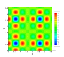
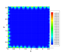
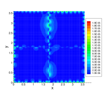
(a) (b) (d)

Figure 45: 2D Helmholtz equation: (a) Solution distribution. Distributions of the absolute error obtained using one sub-domain (b) and using $4$ sub-domains (c) in locELM simulation.

On each sub-domain, we employ a local neural network consisting of an input layer with two nodes (representing $x$ and $y$), a single hidden layer with $M$ nodes and the $\tanh$ activation function, and an output layer with one node (representing $u$). The output layer is linear, with no bias and no activation function. An additional affine mapping normalizing the input $x$ and $y$ data to the interval $[-1,1]\times[-1,1]$ has been incorporated right behind the input layer for all sub-domains. The weight and bias coefficients in the hidden layers are set to uniform random values generated on the interval $[-R_{m},R_{m}]$.

The simulation parameters include the number of sub-domains ($N_{x}$, $N_{y}$, $N_{e}$), the number of collocation points per sub-domain ($Q_{x}$, $Q_{y}$, $Q$), the number of training parameters per sub-domain ($M$), and the maximum magnitude of the random coefficients ($R_{m}$). We employ a fixed seed value $1$ for the Tensorflow random number generator for all the tests in this subsection.

Figure 45 depicts the field distributions of the locELM solution (a), and the absolute errors of the solution computed using one sub-domain (b) and $4$ uniform sub-domains (c). The case with one sub-domain in locELM computation is equivalent to the configuration of a global ELM. In this case, we have employed a total of $Q=50\times 50$ uniform collocation points in the domain, $M=1600$ training parameters in the neural network, and $R_{m}=2.0$ when generating the random weight/bias coefficients for the hidden layers. For the case with $4$ sub-domains, we have partitioned the domain into $2$ sub-domains in each direction ($N_{x}=N_{y}=2$), and employed $Q=25\times 25$ uniform collocation points in each sub-domain (i.e. $Q_{x}=Q_{y}=25$), $M=400$ training parameters per sub-domain, and $R_{m}=1.5$ when generating the random weight/bias coefficients. Therefore the total degrees of freedom for these two cases, i.e. the number of collocation points and the number of training parameters in the domain, are the same. These simulations have both captured the solution accurately. The resultant errors are also comparable, with the case of $4$ sub-domains slightly better.

Figure 46 shows the effect of the degrees of freedom on the locELM accuracy. The effect of varying the number of sub-domains, with the degrees of freedom per sub-domain fixed, is illustrated in Figure 46(a). In this group of tests, we employ $Q=25\times 25$ uniform collocation points/sub-domain ($Q_{x}=Q_{y}=25$), $M=400$ training parameters/sub-domain, and $R_{m}=1.5$ for generating the random weight/bias coefficients. The domain is partitioned into one to nine sub-domains. Figure 46(a) shows the maximum and rms errors in the domain versus the number of sub-domains in the locELM simulation. We can observe that the errors decrease essentially exponentially with increasing number of sub-domains.

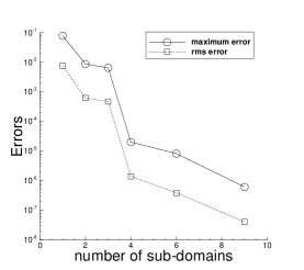
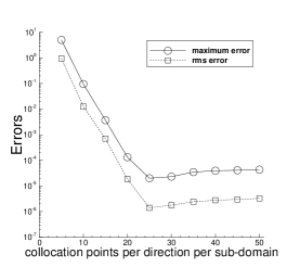
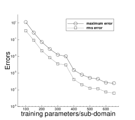
(a) (b) (c)

Figure 46: Effect of degrees of freedom (2D Helmholtz equation): the maximum/rms errors in the domain as a function of (a) the number of sub-domains, (b) the number of collocation points per direction per sub-domain, and (c) the number of training parameters per sub-domain. In (b,c) four sub-domains are used.

The effect of varying the number of collocation points or the number of training parameters per sub-domain is illustrated in Figures 46(b) and (c). In this group of tests we have employed four uniform sub-domains ($N_{x}=N_{y}=2$), and $R_{m}=1.5$ when generating the random weight/bias coefficients, while the number of collocation points/sub-domain or the number of training parameters/sub-domain is varied systematically. Figure 46(b) depicts the maximum and rms errors in the domain as a function of the number of uniform collocation points in each direction ($Q_{x}=Q_{y}$) per sub-domain, where the number of training parameters per sub-domain is fixed at $M=400$. It can be observed that the errors initially decrease exponentially with increasing collocation points, until the number of collocation points reaches a certain level. Then the errors stagnate, and remains essentially the same as the number of collocation points further increases. Figure 46(c) shows the maximum and rms errors in the domain as a function of the training parameters per sub-domain, where the number of uniform collocation points per sub-domain is fixed at $30\times 30$ ($Q_{x}=Q_{y}=30$). It is observed that the errors decrease dramatically with increasing training parameters per sub-domain. The error reduction rate is nearly exponential initially, and the reduction slows down as the number of training parameters/sub-domain becomes large. These results show that the locELM method exhibits a clear sense of convergence with increasing degrees of freedom. The locELM errors decrease essentially exponentially as the number of sub-domains, or the number of collocation points in each direction per sub-domain, or the number training parameters per sub-domain increases.

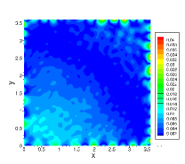
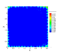
(a) (b)

Figure 47: PINN solution of 2D Helmholtz equation: Field distributions of and the absolute errors obtained using PINN RaissiPK2019 with the Adam optimizer (a) and the L-BFGS optimizer (b). This figure can be compared with Figure 45, which is obtained using the current locELM method.

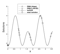
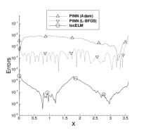
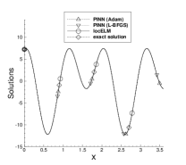
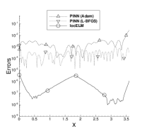
(a) (b) (c) (d)

Figure 48: Comparison between locELM and PINN (2D Helmholtz equation): profiles of the solutions (a,c) and their absolute errors (b,d) along two horizontal lines across the domain at $y=1.0$ (a,b) and $y=2.6$ (c,d), obtained using PINN RaissiPK2019 with the Adam/L-BFGS optimizers and using locELM with 4 sub-domains. The PINN results correspond to Figure 47. The locELM results correspond to Figure 45(c,d).

We next compare the locELM method with PINN RaissiPK2019 for solving the 2D Helmholtz equation. Figure 47 shows the field distributions of the solutions and their errors obtained using PINN together with the Adam and L-BFGS optimizers. The input data consist of $50\times 50$ uniform points in the domain. For the Adam optimizer, the neural network contains $5$ hidden layers, with a width of $40$ nodes for each layer and the $\tanh$ activation function. The neural network has been trained on the input data for $107,000$ epochs, with the learning rate gradually decreasing from $0.001$ at the beginning to $10^{-5}$ at the end of training. For the L-BFGS optimizer, the neural network contains $4$ hidden layers, with a width of $50$ nodes for each layer and the $\tanh$ activation function. The network has been trained on the input data for $24,500$ L-BFGS iterations. The L-BFGS result is observed to be generally more accurate than the Adam result. The results in this figure can be compared with those of Figure 45, which are obtained using the current locELM method. The field distributions indicate that the locELM results are considerably more accurate than the PINN results.

Figure 48 shows a comparison of the solution and error profiles along two horizontal lines across the domain, at $y=1.0$ and $y=2.6$, obtained using PINN and using the current locELM method (with $4$ sub-domains). The superior accuracy of the current method is evident.

method	maximum error	rms error	epochs/iterations	training time (seconds)
PINN (Adam)	$4.13e-2$	$3.91e-3$	$107,000$	$7213.7$
PINN (L-BFGS)	$1.27e-2$	$9.25e-4$	$24,500$	$5051.2$
global ELM	$4.17e-5$	$4.54e-6$	$0$	$410.6$
locELM (4 sub-domains)	$2.01e-5$	$1.41e-6$	$0$	$33.6$

Table 11: 2D Helmholtz equation: comparison between locELM and PINN in terms of the accuracy (maximum/rms errors in domain) and the computational cost (epochs/iterations and the training time). The PINN results correspond to those in Figure 47. The locELM results correspond to those in Figure 45.

Table 11 is a further comparison between the current locELM method and PINN in terms of the maximum and rms errors in the domain, the number of epochs or iterations during the training, and the network training time. The PINN results with the Adam/L-BFGS optimizers correspond to those from Figure 47. The global ELM results correspond to those in Figure 45(a,b), and the locELM results with $4$ sub-domains correspond to those in Figure 45(c,d). Note that the input data for all these cases (PINN and locELM) are the same (total $50\times 50$ uniform collocation points in the domain). It can be observed that the locELM results are two to three orders of magnitude more accurate than the PINN results. In terms of the training time, the current locELM method is much faster than PINN (by over two orders of magnitude). The global ELM method, which is equivalent to the locELM method with one sub-domain, is more than an order of magnitude faster than PINN (around $410$ seconds versus over $5000$ seconds). With $4$ sub-domains, the current locELM method is also much faster than the global ELM (around $33$ seconds versus $410$ seconds). These results clearly signify the superiority of the current method to PINN, in term of both accuracy and the computational cost.

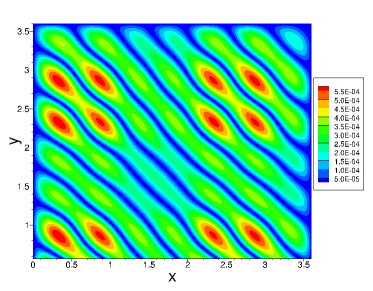
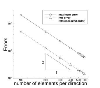
(a) (b)

Figure 49: FEM solution of the 2D Helmholtz equation: (a) FEM error distribution computed on a $590\times 590$ mesh. (b) The FEM maximum/rms errors in the domain versus the number of elements in each direction, showing the second-order convergence rate. On a $N\times N$ mesh, the number of triangular elements is $2N^{2}$.

method	mesh	sub-domains	$Q$	$M$	max-error	rms-error	wall-time (seconds)
FEM	$500\times 500$	–	–	–	$8.20e-4$	$2.00e-4$	$18.5$
	$590\times 590$	–	–	–	$5.89e-4$	$1.51e-4$	$35.4$
locELM	–	$4$	$20\times 20$	$300$	$7.28e-4$	$5.28e-5$	$17.1$
	–	$4$	$25\times 25$	$400$	$2.01e-5$	$1.41e-6$	$33.6$

Table 12: 2D Helmholtz equation: comparison between locELM and the finite element method (FEM) in terms of the maximum/rms errors in the domain and the training or computation time. The FEM results correspond to those in Figure 49. The locELM results correspond to those in Figure 45.

Finally we compare the performance of the current locELM method with the classical finite element method for the 2D Helmholtz equation. Figure 49 illustrates the FEM solution and its second-order convergence rate. Figure 49(a) shows the distribution of the absolute error of the FEM solution computed on a $590\times 590$ uniform rectangular mesh. Note that each rectangle in the mesh is further divided along its diagonal into two triangular linear elements, as stipulated by the FEniCS library. Therefore, in the current work, an $N_{1}\times N_{2}$ rectangular mesh contains a total of $2N_{1}N_{2}$ triangular elements for the FEM simulations. Figure 49(b) shows the maximum/rms errors of the FEM solution in the domain versus the number of rectangles in each direction in the rectangular mesh, demonstrating the second-order convergence rate of the method.

In Table 12 we compare the locELM method and the finite element method with regard to their accuracy and the computational cost. Here we list the maximum and rms errors in the domain, and the wall time for the training or computation, corresponding to a set of different meshes or simulation parameters obtained using locELM and FEM. We observe that the locELM performance is on par with or better than that of the FEM. For example, the FEM case with the $500\times 500$ mesh and the locELM case with $Q=20\times 20$ and $M=300$ have a comparable computational cost and also a similar accuracy. The FEM case with the $590\times 590$ mesh has a comparable computational cost to the locELM case with $Q=25\times 25$ and $M=400$, but its errors are over an order of magnitude larger than those of the latter.

References

- [1] S. Balasundaram and Kapil. Application of error minimized extreme learning machine for simultaneous learning of a function and its derivativs. Neurocomputing, 74:2511–2519, 2011.
- [2] A.G. Baydin, B.A. Pearlmutter, A.A. Radul, and J.M. Siskind. Automatic differentiation in machine learning: a survey. J. Mach. Learn. Res., 18:1–43, 2018.
- [3] N.E. Cotter. The stone-weierstrass theorem and its application to neural networks. IEEE Transactions on Neural Networks, 4:290–295, 1990.
- [4] S. Dong. BDF-like methods for nonlinear dynamic analysis. Journal of Computational Physics, 229:3019–3045, 2010.
- [5] S. Dong. Multiphase flows of N immiscible incompressible fluids: a reduction-consistent and thermodynamically-consistent formulation and associated algorithm. Journal of Computational Physics, 361:1–49, 2018.
- [6] S. Dong and N. Ni. A method for representing periodic functions and enforcing exactly periodic boundary conditions with deep neural networks. arXiv:2007.07442, 2020.
- [7] S. Dong and J. Shen. A time-stepping scheme involving constant coefficient matrices for phase field simulations of two-phase incompressible flows with large density ratios. Journal of Computational Physics, 231:5788–5804, 2012.
- [8] S. Dong and J. Shen. A pressure correction scheme for generalized form of energy-stable open boundary conditions for incompressible flows. Journal of Computational Physics, 291:254–278, 2015.
- [9] S. Dong and Z. Yosibash. A parallel spectral element method for dynamic three-dimensional nonlinear elasticity problems. Computers and Structures, 87:59–72, 2009.
- [10] V. Dwivedi and B. Srinivasan. Physics informed extreme learning machine (pielm) a rapid method for the numerical solution of partial differential equations. Neurocomputing, 391:96–118, 2020.
- [11] W. E and B. Yu. The deep Ritz method: a deep learning-based numerical algorithm for solving variational problems. Communications in Mathematics and Statistics, 6:1–12, 2018.
- [12] G.H. Golub and C.F.V. Loan. Matrix Computations, 3rd Ed. Johns Hopkins Press, MD, 1996.
- [13] I. Goodfellow, Y. Bengio, and A. Courville. Deep Learning. The MIT Press, 2016.
- [14] S. Haykin. Neural Networks: A Comprehensive Foundation. Prentice Hall, 1999.
- [15] J. He and J. Xu. MgNet: A unified framework for multigrid and convolutional neural network. Science China Mathematics, 62:1331–1354, 2019.
- [16] K. Hornik, M. Stinchcombe, and H. White. Multilayer feedforward networks are universal approximators. Neural Networks, 2:359–366, 1989.
- [17] K. Hornik, M. Stinchcombe, and H. White. Universal approximation of an unknown mapping and its derivatives using multilayer feedforward networks. Neural Networks, 3:551–560, 1990.
- [18] G.-B. Huang, D.H. Wang, and Y. Lan. Extreme learning machines: a survey. Int. J. Mach. Learn. Cybern., 2:107–122, 2011.
- [19] G.-B. Huang, Q.-Y. Zhu, and C.-K. Siew. Extreme learning machine: theory and applications. Neurocomputing, 70:489–501, 2006.
- [20] B. Igelnik and Y.H. Pao. Stochastic choice of basis functions in adaptive function approximation and the functional-link net. IEEE Transactions on Neural Networks, 6:1320–1329, 1995.
- [21] H. Jaeger, M. Lukosevicius, D. Popovici, and U. Siewert. Optimization and applications of echo state networks with leaky integrator neurons. Neural Networks, 20:335–352, 2007.
- [22] A.D. Jagtap, E. Kharazmi, and G.E. Karniadakis. Conservative physics-informed neural networks on discrete domains for conservation laws: applications to forward and inverse problems. Computer Methods in Applied Mechanics and Engineering, 365:113028, 2020.
- [23] G.E. Karniadakis and S.J. Sherwin. Spectral/hp element methods for computational fluid dynamics, 2nd edn. Oxford University Press, 2005.
- [24] D.P. Kingma and J. Ba. Adam: a method for stochastic optimization. arXiv:1412.6980, 2014.
- [25] I.E. Lagaris, A.C. Likas, and D.I. Fotiadis. Artificial neural networks for solving ordinary and partial differential equations. IEEE Transactions on Neural Networks, 9:987–1000, 1998.
- [26] I.E. Lagaris, A.C. Likas, and D.G. Papageorgiou. Neural-network methods for boundary value problems with irregular boundaries. IEEE Transactions on Neural Networks, 11:1041–1049, 2000.
- [27] K. Li, K. Tang, T. Wu, and Q. Liao. D3M: A deep domain decomposition method for partial differential equations. IEEE Access, 8:5283–5294, 2020.
- [28] X. Li. Simultaneous approximations of mulvariate functions and their derivatives by neural networks with one hidden layer. Neurocomputiing, 12:327–343, 1996.
- [29] H. Liu, B. Xing, Z. Wang, and L. Li. Legendre neural network method for several classes of singularly perturbed differential equations based on mapping and piecewise optimization technology. Neural Processing Letters, 51:2891–2913, 2020.
- [30] W. Maass and H. Markram. On the computational power of recurrent circuits of spiking neurons. J. Comput.Syst. Sci., 69:593–616, 2004.
- [31] J. Nocedal and S.J. Wright. Numerical Optimization, Second Edition. Springer, 2006.
- [32] S. Panghal and M. Kumar. Optimization free neural network approach for solving ordinary and partial differential equations. Engineering with Computers, Early Access, February 2020.
- [33] Y.H. Pao, G.H. Park, and D.J. Sobajic. Learning and generalization characteristics of the random vector functional-link net. Neurocomputing, 6:163–180, 1994.
- [34] M. Raissi, P. Perdikaris, and G.E. Karniadakis. Physics-informed neural networks: a deep learning framework for solving forward and inverse problems involving nonlinear partial differential equations. Journal of Computational Physics, 378:686–707, 2019.
- [35] F. Rosenblatt. The perceptron: a probabilistic model for information storage and organization in the brain. Psychol. Rev., 65:386–408, 1958.
- [36] K. Rudd and S. Ferrari. A constrained integration (CINT) approach to solving partial differential equations using artificial neural networks. Neurocomputing, 155:277–285, 2015.
- [37] E. Samanaiego, C. Anitescu, S. Goswami, V.M. Nguyen-Thanh, H. Guo, K. Hamdia, X. Zhuang, and T. Rabczuk. An energy approach to the solution of partial differential equations in computational mechanics via machine learning: concepts, implementation and applications. Computer Methods in Applied Mechanics and Engineering, 362:112790, 2020.
- [38] J. Sirignano and K. Spoliopoulos. DGM: A deep learning algorithm for solving partial differential equations. Journal of Computational Physics, 375:1339–1364, 2018.
- [39] Barry F. Smith, Petter E. Bjørstad, and William D. Gropp. Domain decomposition : parallel multilevel methods for elliptic partial differential equations. Cambridge University Press, 1996.
- [40] H. Sun, M. Hou, Y. Yang, T. Zhang, F. Weng, and F. Han. Solving partial differential equations based on bernsteirn neural network and extreme learning machine algorithm. Neural Processing Letters, 50:1153–1172, 2019.
- [41] A. Toselli and O. Widlund. Domain Decomposition Methods Algorithms and Theory. Springer, 2005.
- [42] C.S. Webster. Alan Turing’s unorganized machines and artificial neural networks: his remarkable early work and future possibilities. Evol. Intel., 5:35–43, 2012.
- [43] P.J. Werbos. Beyond regression: new tools for prediction and alaysis in the behavioral sciences. PhD Thesis, Harvard Univeristy, Cambridge, MA, 1974.
- [44] J. Xu. The finite neuron method and convergence analysis. arXiv:2010.01458, 2020.
- [45] Y. Yang, M. Hou, and J. Luo. A novel improved extreme learning machine algorithm in solving ordinary differential equations by legendre neural network methods. Advances in Differential Equations, 469:1–24, 2018.
- [46] Y. Zang, G. Bao, X. Ye, and H. Zhou. Weak adversarial networks for high-dimensional partial differential equations. Journal of Computational Physics, 411:109409, 2020.
- [47] L. Zhang and P.N. Suganthan. A comprehensive evaluation of random vector functional link networks. Inf. Sci., 367–368:1094–1105, 2016.
- [48] X. Zheng and S. Dong. An eigen-based high-order expansion basis for structured spectral elements. Journal of Computational Physics, 230:8573–8602, 2011.