Encoding the latent posterior of Bayesian Neural Networks for uncertainty quantification

Abstract

Bayesian Neural Networks (BNNs) have been long considered an ideal, yet unscalable solution for improving the robustness and the predictive uncertainty of deep neural networks. While they could capture more accurately the posterior distribution of the network parameters, most BNN approaches are either limited to small networks or rely on constraining assumptions, e.g., parameter independence. These drawbacks have enabled prominence of simple, but computationally heavy approaches such as Deep Ensembles, whose training and testing costs increase linearly with the number of networks. In this work we aim for efficient deep BNNs amenable to complex computer vision architectures, e.g., ResNet50 DeepLabV3+, and tasks, e.g., semantic segmentation, with fewer assumptions on the parameters. We achieve this by leveraging variational autoencoders (VAEs) to learn the interaction and the latent distribution of the parameters at each network layer. Our approach, Latent-Posterior BNN (LP-BNN), is compatible with the recent BatchEnsemble method, leading to highly efficient (in terms of computation and memory during both training and testing) ensembles. LP-BNNs attain competitive results across multiple metrics in several challenging benchmarks for image classification, semantic segmentation and out-of-distribution detection.

1 Introduction

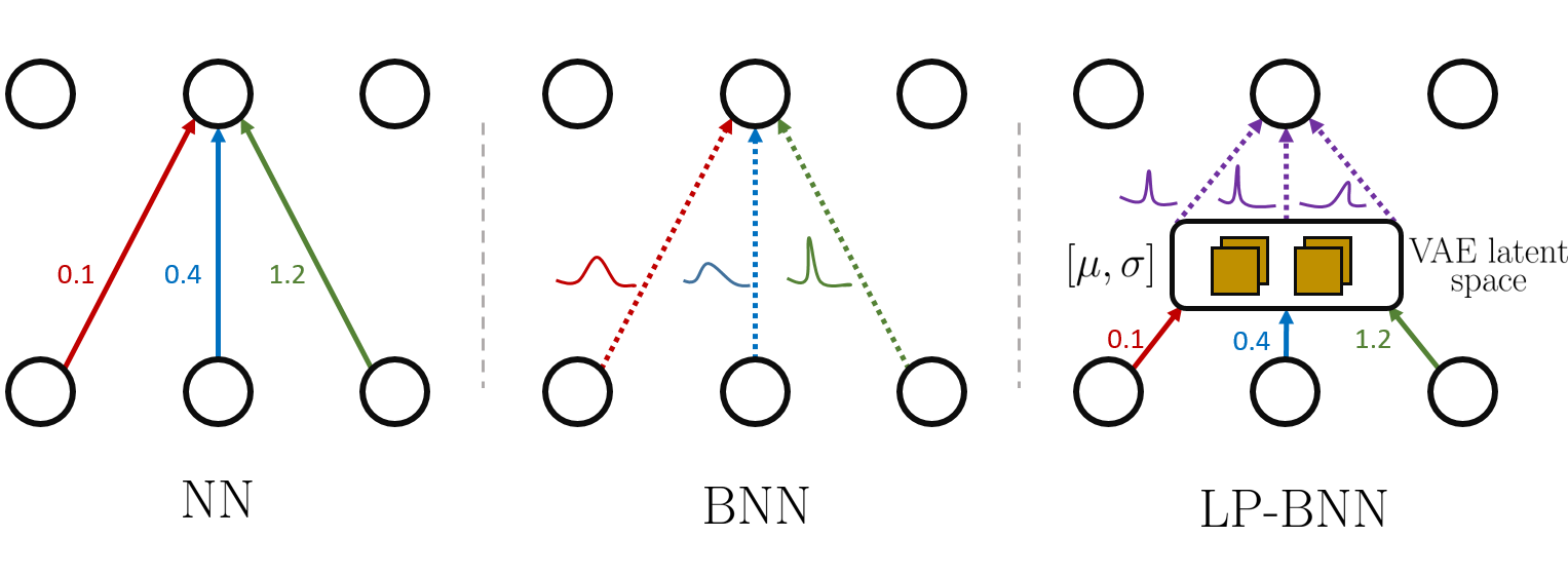
Figure 1: In a standard NN each weight has a fixed value. In most BNNs all weights follow Gaussian distributions and are assumed to be mutually independent: each weight is factorized by a Gaussian distribution. For LP-BNN in each layer, weights follow a multivariate Gaussian distribution with a latent weight space composed of independent Gaussian distributions. This enables computing expressive weight distributions in a lower dimensional space.

Most top-performing approaches for predictive uncertainty estimation with Deep Neural Networks (DNNs) [39, 2, 45, 15] are essentially based on ensembles, in particular Deep Ensembles (DE) [39], which have been shown to display many strengths: stability, mode diversity, good calibration, etc. [13]. In addition, through the Bayesian lens, ensembles enable a more straightforward separation and quantification of the sources and forms of uncertainty [16, 39, 47], which in turn allows a better communication of the decisions to humans [5, 37] or to connected modules in an autonomous system [49]. This is crucial for real-world decision making systems. Although originally introduced as simple and scalable alternative to Bayesian Neural Networks (BNNs) [44, 52], DE still have notable drawbacks in terms of computational cost for both training and testing often make them prohibitive in practical applications.

In this work we address uncertainty estimation with BNNs, the departure point of DE. BNNs propose an intuitive and elegant formalism suited for this task by estimating the posterior distribution over the parameters of a network conditioned on training data. Performing exact inference BNNs is intractable and most approaches require approximations. The most common one is the mean-field assumption [33], i.e., the weights are assumed to be independent of each other and factorized by their own distribution, usually Gaussian [27, 19, 6, 26, 17, 51]. However, this approximation can be damaging [44, 12] as a more complex organization can emerge within network layers, and that higher level correlations contribute to better performance and generalization [4, 62, 64]. Yet, even under such settings, BNNs are challenging to train at scale on modern DNN architectures [54, 10]. In response, researchers have looked into structured-covariance approximations [42, 65, 76, 51], however they further increase memory and time complexity over the original mean-field approximation.

Here, we revisit BNNs in a pragmatic manner. We propose an approach to estimate the posterior of a BNN with layer-level inter-weight correlations, in a stable and computationally efficient manner, compatible with modern DNNs and complex computer vision tasks, e.g., semantic segmentation. We advance a novel deep BNN model, dubbed Latent Posterior BNN (LP-BNN), where the posterior distribution of the weights at each layer is encoded with a variational autoencoder (VAE) [36] into a lower-dimensional latent space that follows a Gaussian distribution (see Figure 1). We switch from the inference of the posterior in the high dimensional space of the network weights to a lower dimensional space which is easier to learn and already encapsulates weight interaction information. LP-BNN is naturally compatible with the recent BatchEnsemble (BE) approach [70] that enables learning a more diverse posterior from the weights of the BE sub-networks. Their combination outperforms most of related approaches across a breadth of benchmarks and metrics. In particular, LP-BNN is competitive with DE and has significantly lower costs for training and prediction.

Contributions.   To summarize, the contributions of our work are: (1) We introduce a scalable approach for BNNs to implicitly capture layer-level weight correlations enabling more expressive posterior approximations, by foregoing the limiting mean-field assumption LP-BNN scales to high capacity DNNs (e.g., 50+ layers and 30M parameters for DeepLabv3+), while still training on a single V100 GPU. (2) We propose to leverage VAEs for computing the posterior distribution of the weights by projecting them in the latent space. This improves significantly training stability while ensuring diversity of the sampled weights. (3) We extensively evaluate our method on a range of computer vision tasks and settings: image classification for in-domain uncertainty, out-of-distribution (OOD) detection, robustness to distribution shift, and semantic segmentation ( high-resolution images, strong class imbalance) for OOD detection. We demonstrate that LP-BNN achieves similar performances with high-performing Deep Ensembles, while being substantially more efficient computationally.

2 Background

In this section, we present the chosen formalism for this work and offer a short background on BNNs.

2.1 Preliminaries

We consider a training dataset $\mathcal{D}=\{(\mathbf{x}_{i},y_{i})\}_{i=1}^{n}$ with $n$ samples and labels, corresponding to two random variables $X\sim\mathcal{P}_{X}$ and $Y\sim\mathcal{P}_{Y}$. Without loss of generality we represent $\mathbf{x}_{i}\in^{d}$ as a vector, and $y_{i}$ as a scalar label. We process the input data $\mathbf{x}_{i}$ with a neural network $f_{\Theta}(\cdot)$ with parameters $\Theta$, that outputs a classification or regression prediction. We view the neural network as a probabilistic model with $f_{\Theta}(\mathbf{x}_{i})=P(Y=y_{i}\mid X=\mathbf{x}_{i},\Theta)$. In the following, when there are no ambiguities, we discard the random variable from notations. For classification, $P(y_{i}\mid\mathbf{x}_{i},\Theta)$ is a categorical distribution over the set of classes over the domain of $Y$, typically corresponding to the cross-entropy loss function, while for regression $P(y_{i}\mid\mathbf{x}_{i},\Theta)$ is a Gaussian distribution of real values over the domain of $Y$ when using the squared loss function. For simplicity we unroll our reasoning for the classification task.

In supervised learning, we leverage gradient descent for learning $\Theta$ that minimizes the cross-entropy loss, which is equivalent to finding the parameters that maximize the likelihood estimation (MLE) $P(\mathcal{D}\mid\Theta)$ over the training set $\Theta_{\text{MLE}}=\arg\max_{\Theta}\sum_{(\mathbf{x}_{i},y_{i})\in\mathcal{D}}\log P(y_{i}\mid\mathbf{x}_{i},\Theta)$, or equivalently minimize the following loss function:

$$\mathcal{L}_{\scriptscriptstyle\text{MLE}}(\Theta)=-\sum_{(\mathbf{x}_{i},y_{i})\in\mathcal{D}}\log P(y_{i}\mid\mathbf{x}_{i},\Theta).$$ (1)

The Bayesian approach enables adding prior information on the parameters $\Theta$, by placing a prior distribution $\mathcal{P}(\Theta)$ upon them. This prior represents some expert knowledge about the dataset and the model. Instead of maximizing the likelihood, we can now find the maximum a posteriori (MAP) weights for $\mathcal{P}(\Theta\mid\mathcal{D})\propto\mathcal{P}(\mathcal{D}\mid\Theta)\mathcal{P}(\Theta)$ to compute $\Theta_{\text{MAP}}=\arg\max_{\Theta}\sum_{(\mathbf{x}_{i},y_{i})\in\mathcal{D}}\log\mathcal{P}(y_{i}\mid\mathbf{x}_{i},\Theta)+\log\mathcal{P}(\Theta)$, i.e. to minimize the following loss function:

$$\mathcal{L}_{\scriptscriptstyle\text{MAP}}(\Theta)=-\sum_{(\mathbf{x}_{i},y_{i})\in\mathcal{D}}\log P(y_{i}\mid\mathbf{x}_{i},\Theta)-\log P(\Theta),$$ (2)

inducing a specific distribution over the functions computed by the network and a regularization of the weights. For a Gaussian prior, Eq. (2) reads as $L_{2}$ regularization (weight decay).

2.2 Bayesian Neural Networks

In most neural networks only the $\Theta_{\text{MAP}}$ weights computed during training are kept for predictions. Conversely, in BNNs we aim to find the posterior distribution $P(\Theta\mid\mathcal{D})$ of the parameters given the training dataset, not only the values corresponding to the MAP. Here we can make a prediction $y$ on a new sample $\mathbf{x}$ by computing the expectation of the predictions from an infinite ensemble corresponding to different configurations of the weights sampled from the posterior distribution:

$$P(y\mid\mathbf{x},\mathcal{D})=\int P(y\mid\mathbf{x},\Theta)P(\Theta\mid\mathcal{D})d\Theta,$$ (3)

which is also known as Bayes ensemble. The integral in Eq. (3), which is calculated over the domain of $\Theta$, is intractable, and in practice it is approximated by averaging predictions from a limited set $\{\Theta_{1},\ldots\Theta_{J}\}$ of $J$ weight configurations sampled from the posterior distribution:

$$P(y\mid\mathbf{x},\mathcal{D})\approx\frac{1}{J}\sum_{j=1}^{J}P(y\mid\mathbf{x},\Theta_{j}).$$ (4)

Although BNNs are elegant and easy to formulate, their inference is non-trivial and has been subject to extensive research across the years [27, 44, 52]. Early approaches relied on Markov chain Monte Carlo variants for inference, while progress in variational inference (VI) [33] has enabled a recent revival of BNNs [19, 6, 26]. VI turns posterior inference into an optimization problem. In detail, VI finds the parameters $\nu$ of a distribution $Q_{\nu}(\Theta)$ on the weights that approximates the true Bayesian posterior distribution of the weights $P(\Theta\mid\mathcal{D})$ through KL-divergence minimization. This is equivalent to minimizing the following loss function, also known as expected lower bound (ELBO) loss [6, 36]:

$$\mathcal{L}_{\scriptscriptstyle\text{BNN}}(\Theta,\nu)= -\sum_{(\mathbf{x}_{i},y_{i})\in\mathcal{D}}\mathbb{E}_{\scriptstyle{\color[rgb]{0,0,0}\Theta\sim}Q_{\nu}(\Theta)}\log\left(P(y_{i}\mid\mathbf{x}_{i},\Theta)\right)$$

$$+\mbox{KL}(Q_{\nu}(\Theta)||P(\Theta)).$$ (5)

The loss function $\mathcal{L}_{\scriptscriptstyle\text{BNN}}(\Theta,\nu)$ is composed of two terms: the KL term depends on the weights and the prior $P(\Theta)$, while the likelihood term is data dependent. This function strives to simultaneously capture faithfully the complexity and diversity of the information from data $\mathcal{D}$, while preserving the simplicity of the prior $P(\Theta)$. To optimize this loss function, Blundell et al. [6] proposed leveraging the re-parameterization trick [36, 60], foregoing the expensive MC estimates.

Discussion.

BNNs are particularly appealing for uncertainty quantification thanks to the ensemble of predictions from multiple weight configurations sampled from the posterior distribution. However this brings an increased computational and memory cost. For instance, the simplest variant of BNNs with fully factorized Gaussian approximation distributions [6, 19], i.e. each weight consists of a Gaussian mean and variance, carries a double amount of parameters. In addition, recent works [54, 10] point out that BNNs often underfit, and need multiple tunings to stabilize training dynamics involved by the loss function and the variance from weight samplings at each forward pass. Due to computational limitations, most BNN approaches assume that parameters are not correlated. This hinders their effectiveness [12], as empirical evidence has shown that encouraging weight collaboration improves training stability and generalization [58, 62, 64].

In order to calculate a tractable weight correlation aware posterior distribution, we propose to leverage a VAE to compute compressed latent distributions from which we can sample new weight configurations. We rely on the recent BatchEnsemble (BE) method [70] to further improve the parameter-efficiency of BNNs. We now proceed to describe BE and then derive our approach.

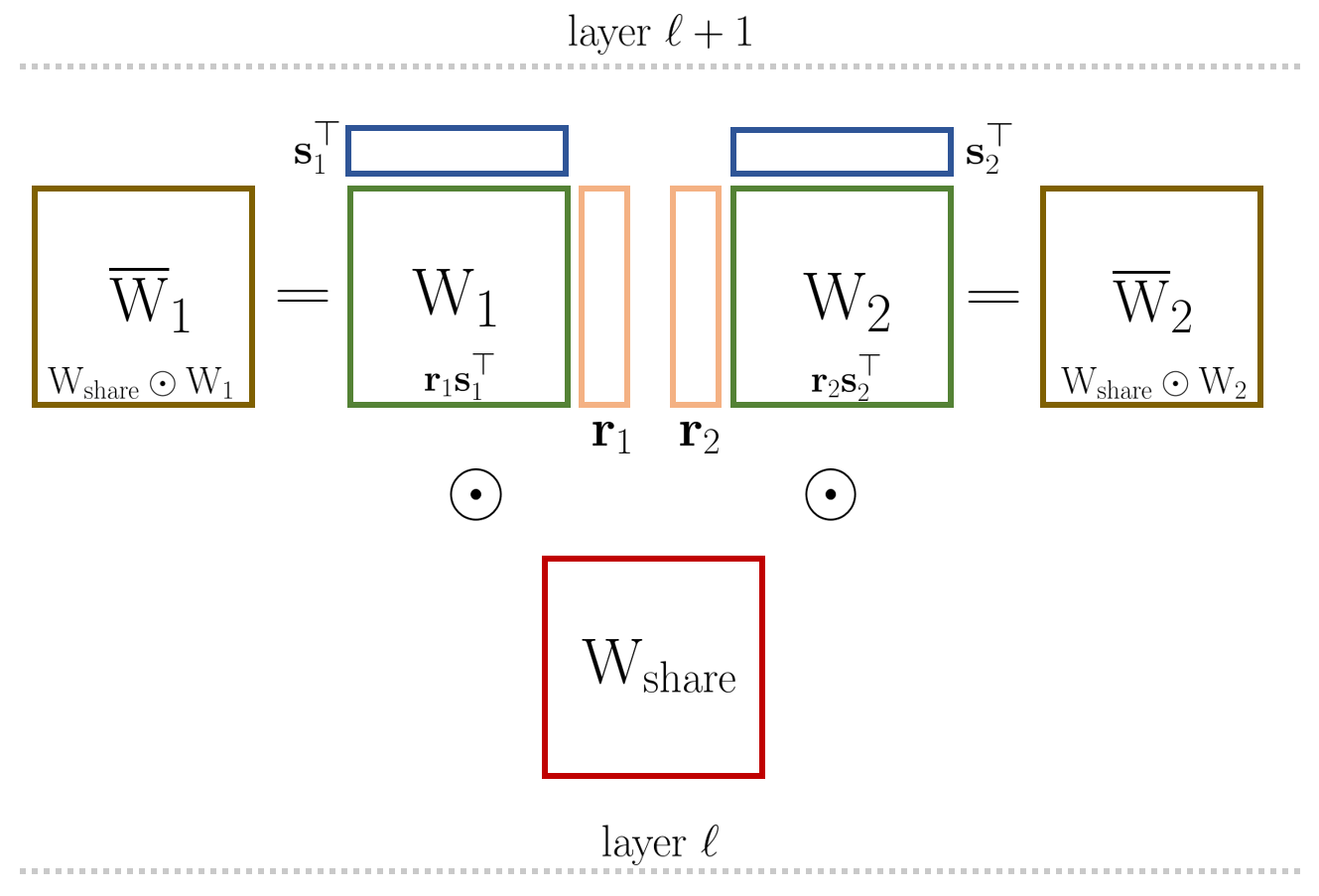
Figure 2: Diagram of a BatchEnsemble layer that generates for an ensemble of size $J{=}2$, the ensemble weights $\overline{\mathbf{W}}_{j}$ from shared weights $\mathbf{W}_{\text{share}}$ and fast weights $\mathbf{W}_{j}{=}\mathbf{r}_{j}\mathbf{s}_{j}^{\top}$, with $j\in\llbracket 1,J\rrbracket$.

2.3 BatchEnsemble

Deep Ensembles (DEs) [39] are a popular and pragmatic alternative to BNNs. While DEs boast outstanding accuracy and predictive uncertainty, their training and testing cost increases linearly with the number of networks. This drawback has motivated the emergence of a recent stream of works proposing efficient ensemble methods [2, 15, 45, 50, 70]. One of the most promising ones is BatchEnsemble [70], which mimics in a parameter-efficient manner one of the main strengths of DE, i.e. diverse predictions [13].

In a nutshell, BE builds up an ensemble from a single base network (shared among ensemble members) and a set of layer-wise weight matrices specific to each member. At each layer, the weight of each ensemble member is generated from the Hadamard product between a weight shared among all ensemble members, called “slow weight”, and a Rank-1 matrix that varies among all members, called “fast weight”. Formally, let $\mathbf{W}_{\text{share}}\in^{m\times p}$ be the slow weights in a neural network layer with input dimension $m$ and with $p$ outputs. Each member $j$ from an ensemble of size $J$ owns a fast weight matrix $\mathbf{W}_{j}\in^{m\times p}$. $\mathbf{W}_{j}$ is a Rank-1 matrix computed from a tuple of trainable vectors $\mathbf{r}_{j}\in^{m}$ and $\mathbf{s}_{j}\in^{p}$, with $\mathbf{W}_{j}=\mathbf{r}_{j}\mathbf{s}_{j}^{\top}$. BE generates from them a family of ensemble weights as follows: $\overline{\mathbf{W}}_{j}=\mathbf{W}_{\text{share}}\odot\mathbf{W}_{j}$, where $\odot$ is the Hadamard product. Each $\overline{\mathbf{W}}_{j}$ member of the ensemble is essentially a Rank-1 perturbation of the shared weights $\mathbf{W}_{\text{share}}$ (see Figure 2). The sequence of operations during the forward pass reads:

$$h=a\left((W_{\text{share}}^{\top}(\mathbf{x}\odot\mathbf{s}_{j}))\odot\mathbf{r}_{j}\right),$$ (6)

where $a$ is an activation function and $h$ the output activations.

The operations in BE can be efficiently vectorized, enabling each member to process in parallel the corresponding subset of samples from the mini-batch. $\mathbf{W}_{\text{share}}$ is trained in a standard manner over all samples in the mini-batch. A BE network $f_{\Theta^{\scriptscriptstyle\text{BE}}}$ is parameterized by an extended set of parameters $\Theta^{\scriptscriptstyle\text{BE}}=\big{\{}\theta^{\text{slow}}:\{\mathbf{W}_{\text{share}}\},\theta^{\text{fast}}:\{\mathbf{r}_{j},\mathbf{s}_{j}\}_{j=1}^{J}\big{\}}$.

With its multiple sub-networks parameterized by a reduced set of weights, BE is a practical method that can potentially improve the scalability of BNNs. We take advantage of the small size of the fast weights to capture efficiently the interactions between units and to compute a latent distribution of the weights. We detail our approach below.

3 Efficient Bayesian Neural Networks (BNNs)

3.1 Encoding the posterior weight distribution of a BNN

Most BNN variants assume full independence between weights, both inter- and intra-layer. Modeling precisely weight correlations in modern high capacity DNNs with thousands to millions of parameters per layer [22] is however a daunting endeavor due to computational intractability. Yet, multiple strategies aiming to boost weight collaboration in one way or another, e.g. Dropout [64], WeightNorm [62], Weight Standardization [58], have proven to improve training speed, stability and generalization. Ignoring weight correlations might partially explain the shortcomings of BNNs in terms of underfitting [54, 10]. This motivates us to find a scalable way to compute the posterior distribution of the weights without discarding their correlations.

Li et al. [41] have recently found that the intrinsic dimension of DNNs can be in the order of hundreds to a few thousands. The good performances of BE, that builds on weights from a low-rank subspace, further confirm this finding. For efficiency, we leverage the Rank-1 subspace decomposition in BE and estimate here the distribution of the weights, leading to a novel form of BNNs. Formally, instead of computing the posterior distribution $P(\Theta\mid\mathcal{D})$, we aim now for $P(\theta^{\text{fast}}\mid\mathcal{D})$.

A first approach would be to compute Rank-1 weight distributions by using $\mathbf{r}_{j}$ and $\mathbf{s}_{j}$ as variational layers, place priors on them and compute their posterior distributions in a similar manner to [6]. Dusenberry et al. [10] show that these Rank-1 BNNs stabilize training by reducing the variance of the sampled weights, due to sampling only from Rank-1 variational distributions instead of full weight matrices. However this raises the memory cost significantly, as training is performed simultaneously over all $J$ sub-networks: on CIFAR-10 for ResNet-50 with $J{=}4$, the authors use $8$ TPUv2 cores with mini-batches of size $64$ per core.

We argue that a more efficient way of computing the posterior distribution of the fast weights would be to learn instead the posterior distribution of the lower dimensional latent variables of $\{\mathbf{r},\mathbf{s}\}\in\theta^{\text{fast}}$. This can be efficiently done with a VAE [36] that can find a variational approximation $Q_{\phi}(\mathbf{z}\mid\mathbf{r})$ to the intractable posterior distribution $P_{\psi}(\mathbf{z}\mid\mathbf{r})$. VAEs can be seen as a generative model that can deal with complicated dependencies between input dimensions via a probabilistic encoder that projects the input into a latent space following a specific prior distribution. For simplicity and clarity, from here onward we derive our formalism only for $\mathbf{r}$ at a single layer and consider weights $\mathbf{s}$ to be deterministic. Here the input to the VAE are the weights $\mathbf{r}$ and we rely on it to learn the dependencies between weights and encode them into the latent representation.

In detail, for each layer of the network $f_{\Theta}(\cdot)$ we introduce a VAE composed of a one layer encoder $g^{\scriptstyle\text{enc}}_{\scriptstyle\phi}(\cdot)$ with variational parameters $\phi$ and a one layer decoder $g^{\scriptstyle\text{dec}}_{\scriptstyle\psi}(\cdot)$ with parameters $\psi$. Let the prior over the latent variables be a centered isotropic Gaussian distribution $P_{\psi}(\mathbf{z})=\mathcal{N}(\mathbf{z};0,\mathbf{I})$. Like common practice, we let the variational approximate posterior distribution $Q_{\phi}(\mathbf{z}\mid\mathbf{r})$ be a multivariate Gaussian with diagonal covariance. The encoder takes as input a mini-batch of size $J$ (the size of the ensemble) composed of all the $\mathbf{r}_{j}$ weights of this layer and outputs as activations $(\bm{\mathbf{\mu}}_{j},\bm{\mathbf{\sigma}}^{2}_{j})$. We sample a latent variable $\mathbf{z}_{j}\sim\mathcal{N}(\bm{\mathbf{\mu}}_{j},\bm{\mathbf{\sigma}}^{2}_{j}\mathbf{I})$ and feed it to the decoder, which in turn outputs the reconstructed weights $\hat{\mathbf{r}}_{j}=g^{\scriptstyle\text{dec}}_{\scriptstyle\psi}(\mathbf{z}_{j})$. In other words, at each forward pass, we sample new fast weights $\hat{\mathbf{r}}_{j}$ from the latent posterior distribution to be further used for generating the ensemble. The weights of each member of the ensemble $\overline{\mathbf{W}}_{j}=\mathbf{W}_{\scriptstyle\text{share}}\odot(\hat{\mathbf{r}}_{j}\mathbf{s}_{j}^{\top})$ are now random variables depending on $\mathbf{W}_{\scriptstyle\text{share}}$, $\mathbf{s}_{j}$ and $\mathbf{z}_{j}$. Note that while in practice we sample $J$ weight configurations, this approach allows us to generate larger ensembles by sampling multiple times from the same latent distribution. We illustrate an overview of an LP-BNN  layer in Figure 3.

The VAE modules are trained in the standard manner with the ELBO loss function [36] jointly with the rest of the network. The final loss function is:

$$\mathcal{L}_{\scriptscriptstyle\text{LP-BNN}}(\Theta^{\scriptscriptstyle\text{LP-BNN}}){=}-\sum_{\scriptscriptstyle(\mathbf{x}_{i},y_{i})\in\mathcal{D}}{\mathbb{E}}_{\scriptscriptstyle\mathbf{z}\sim Q_{\phi}(\mathbf{z}|\mathbf{r})}\log\left(P({y_{i}}\mid\mathbf{x}_{i},\Theta^{\scriptscriptstyle\text{LP-BNN}},\mathbf{z})\right)\\ +1/L\left(\mbox{KL}(Q_{\scriptstyle\phi}(\mathbf{z}\mid\mathbf{r})||P_{\scriptstyle\psi}(\mathbf{z}))+\|\mathbf{r}-\hat{\mathbf{r}}\|^{2}\right),$$ (7)

where $\Theta^{\scriptscriptstyle\text{LP-BNN}}{=}\big{\{}\theta^{\scriptstyle\text{slow}},\theta^{\scriptstyle\text{fast}}{:}\{\mathbf{r}_{j},\mathbf{s}_{j}\}_{j{=}1}^{J},\theta^{\scriptstyle\text{variational}}{:}\{\phi,\psi\}\big{\}}$ and $L$ the number of layers. The loss function is applied to all $J$ members of the ensemble.

At a first glance, the loss function $\mathcal{L}_{\scriptscriptstyle\text{LP-BNN}}$ bears some similarities with $\mathcal{L}_{\scriptscriptstyle\text{BNN}}$ (Eq. 2.2). Both functions include likelihood and KL terms. The likelihood in $\mathcal{L}_{\scriptscriptstyle\text{BNN}}$, i.e. the cross-entropy loss, depends on input data $\mathbf{x}_{i}$ and on the parameters $\Theta$ sampled from $Q_{\nu}(\Theta)$, while $\mathcal{L}_{\scriptscriptstyle\text{LP-BNN}}$ depends on the latent variables $\mathbf{z}_{j}$ sampled from $Q_{\phi}(\mathbf{z}_{j}\mid\mathbf{r}_{j})$ that lead to the fast weights $\hat{\mathbf{r}_{j}}$. It guides the weights towards useful values for the main task. The KL term in $\mathcal{L}_{\scriptscriptstyle\text{BNN}}$ enforces the per-weight prior, while in $\mathcal{L}_{\scriptscriptstyle\text{LP-BNN}}$ it preserves the consistency and simplicity of the common latent distribution of the weights $\mathbf{r}_{j}$. In addition, $\mathcal{L}_{\scriptscriptstyle\text{LP-BNN}}$ has an input weight reconstruction loss (last term in Eq. 7) ensuring that the generated weights $\hat{\mathbf{r}}_{j}$ are still compatible with the rest of parameters of the network and do not cause high variance and instabilities during training, as typically occurs in standard BNNs [10].

At test time, we generate the LP-BNN ensemble on the fly by sampling the weights $\hat{\mathbf{r}}_{j}$ from the encodings of $\mathbf{r}_{j}$ to compute $\overline{\mathbf{W}}_{j}$. For the final prediction we compute the empirical mean of the likelihoods of the ensemble:

$$P(y_{i}|\mathbf{x}_{i})=\frac{1}{J}\sum_{j=1}^{J}P(y_{i}\mid\mathbf{x}_{i},\theta^{\text{slow}},\mathbf{s}_{j},\hat{\mathbf{r}}_{j})$$ (8)

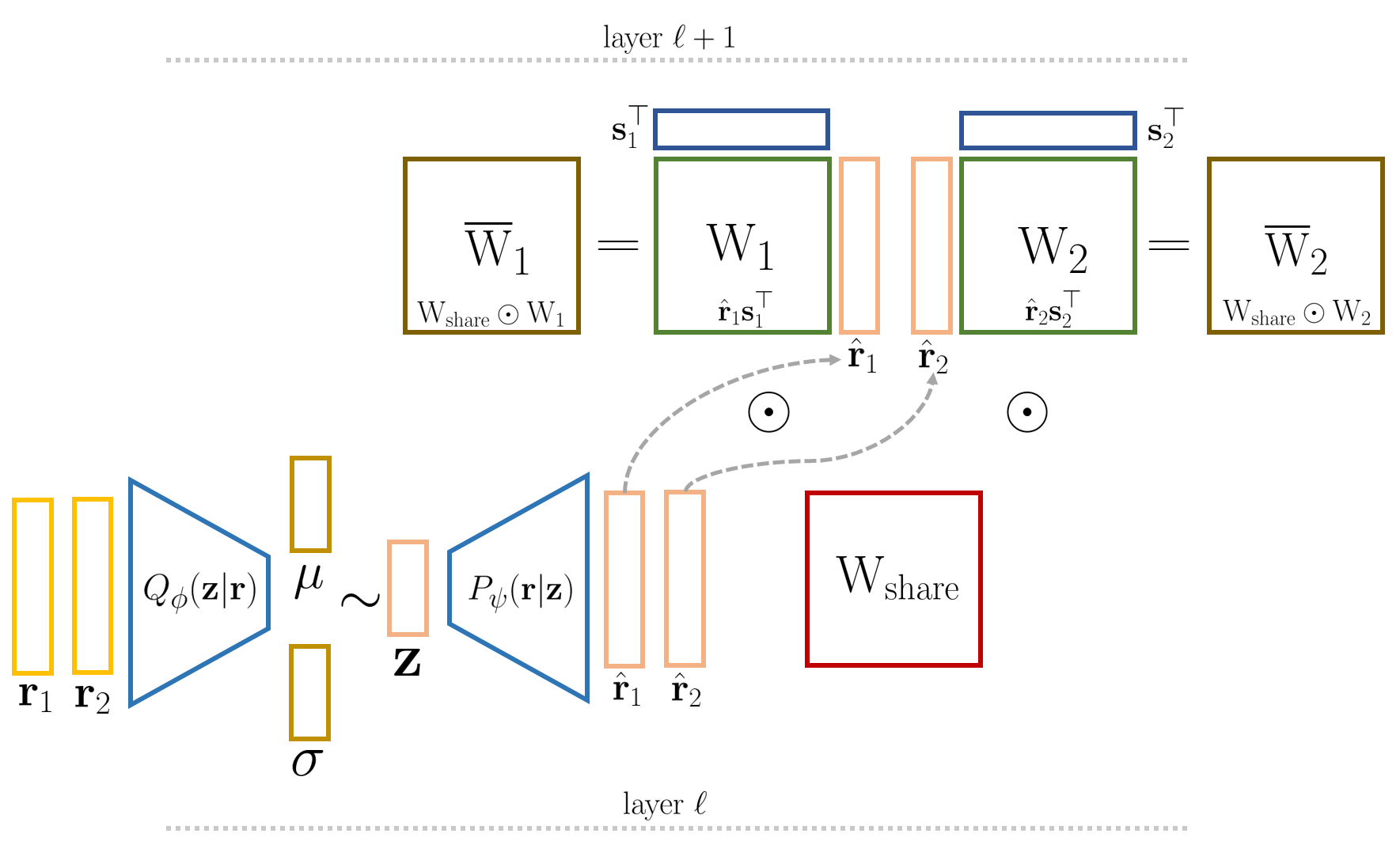
Figure 3: Diagram of a LP-BNN layer that generates for an ensemble of size $J{=}2$, ensemble weights $\overline{\mathbf{W}}_{j}$ from shared weights $\mathbf{W}_{\text{share}}$ and fast weights $\mathbf{s}_{\scriptscriptstyle j}$ and $\hat{\mathbf{r}}_{\scriptscriptstyle j}$, the latter sampled and decoded from the corresponding latent projection $\mathbf{z}_{\scriptscriptstyle j}$ of $\mathbf{r}_{\scriptscriptstyle j}$, with $j\in\llbracket 1,J\rrbracket$.

3.2 Discussion on LP-BNN

We discuss here the quality of the uncertainty from LP-BNN. The predictive uncertainty of a DNN stems from two main types of uncertainty [28]: aleatoric uncertainty and epistemic uncertainty. The former is related to randomness, typically due to the noise in the data. The latter concerns finite size training datasets. The epistemic uncertainty captures the uncertainty in the DNN parameters and their lack of knowledge on the model that generated the training data.

In BNN approaches, through likelihood marginalization over weights, the prediction is computed by integrating the outputs from different DNNs weighted by the posterior distribution (Eq. 3), allowing us to conveniently capture both types of uncertainties [47]. The quality of the uncertainty estimates depends on the diversity of predictions and views provided by the BNN. DE [39] achieve excellent diversity [13] by mimicking BNN ensembles through training of multiple individual models. Recently, Wilson and Izmailov [72] proposed to combine DE and BNNs towards improving diversity further. However, as DE are already computationally demanding, we argue that BE is a more pragmatic choice for increasing the diversity of our BNN, leading to better uncertainty quantification.

Figure S1 shows a qualitative comparison of the prediction diversity from different methods. We compare LP-BNN, BE, and DE based on WRN-28-10 [75] trained on CIFAR-10 [38] and analyze predictions on CIFAR-10, CIFAR10-C [24], and SVHN [53] test images. SVHN contains digits which have a different distribution from the training data, i.e., predominant epistemic uncertainty, while CIFAR10-C displays a distribution shift via noise corruption, i.e., more aleatoric uncertainty. The expected behavior is that individual DNNs in an ensemble would predict different classes for OOD images and have higher entropy on the corrupted ones, reducing the confidence score of the ensemble. We can see that the diversity of BE is lower for CIFAR10-C and SVHN, leading to poorer results in Table 3.

In the supplementary we include additional discussions on our posterior covariance matrix (§A.1), the link between the size of the ensemble and the covariance matrix approximation (§A.2), computational complexity (§A.3), training stability of LP-BNN (§A.4), and diversity of LP-BNN (§A.5).

Input

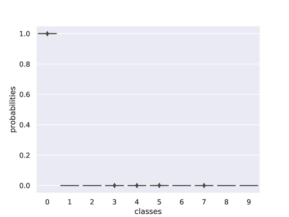
LP-BNN

BE

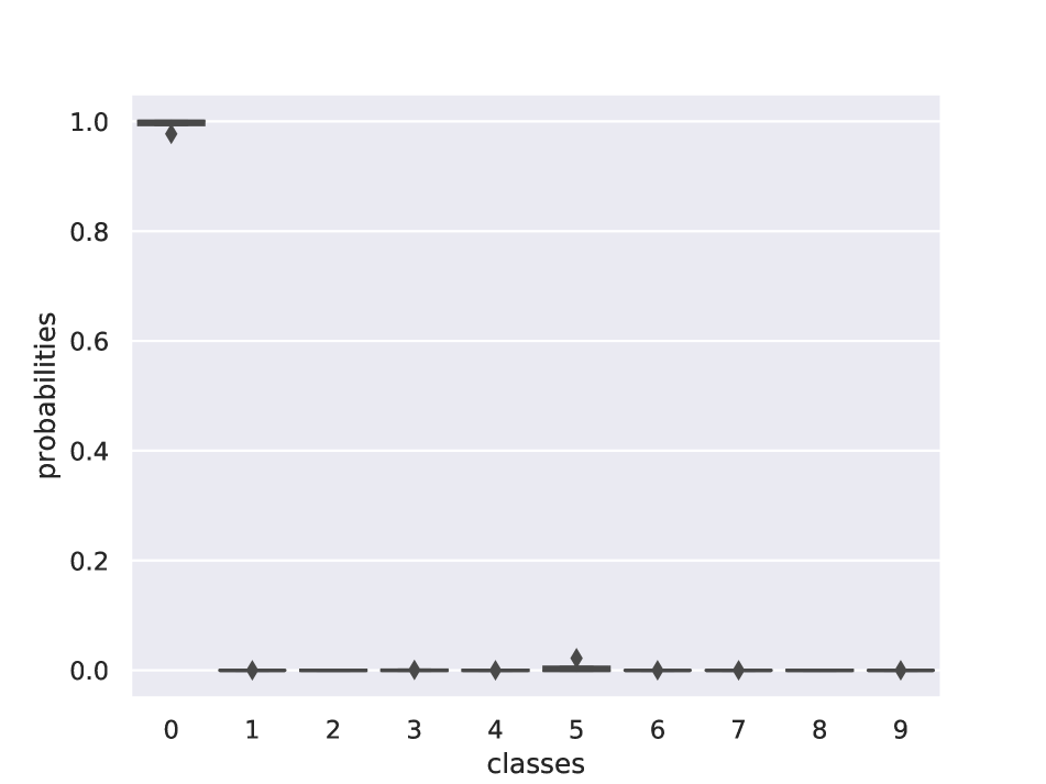
DE

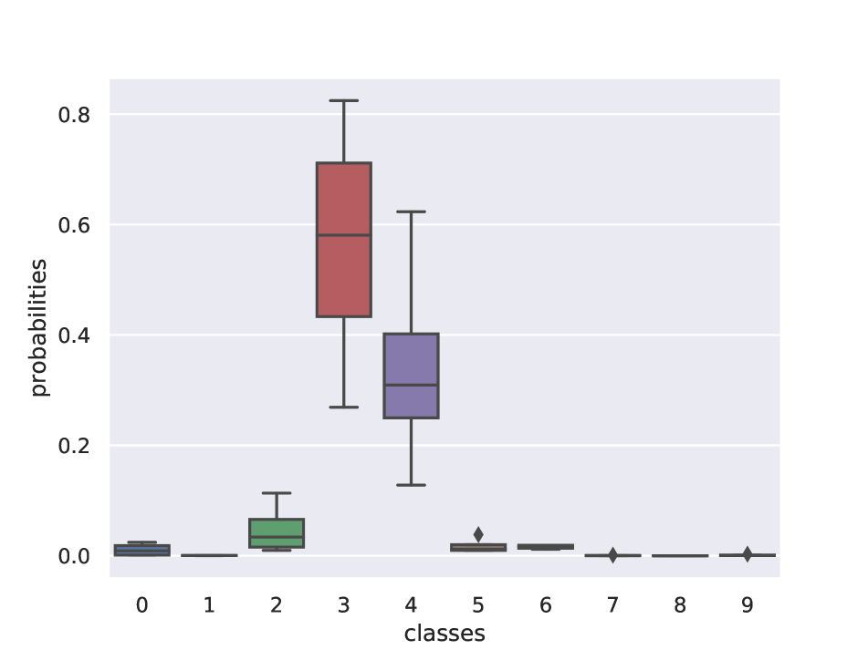
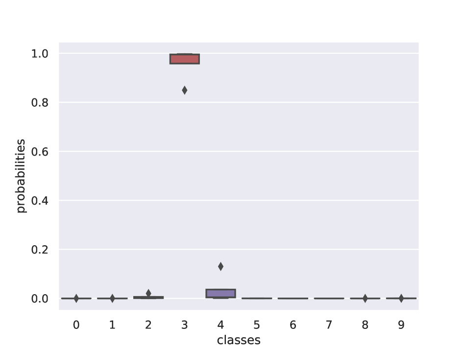
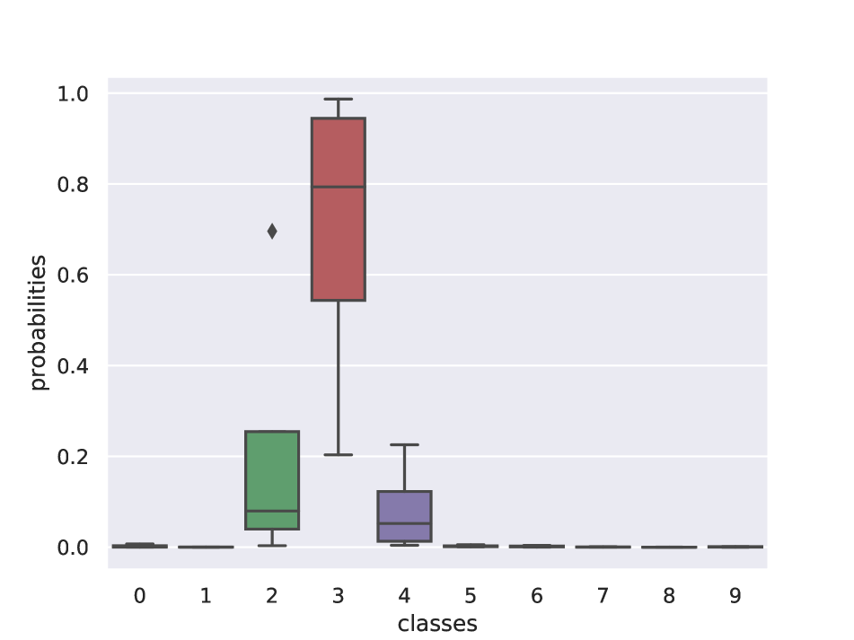
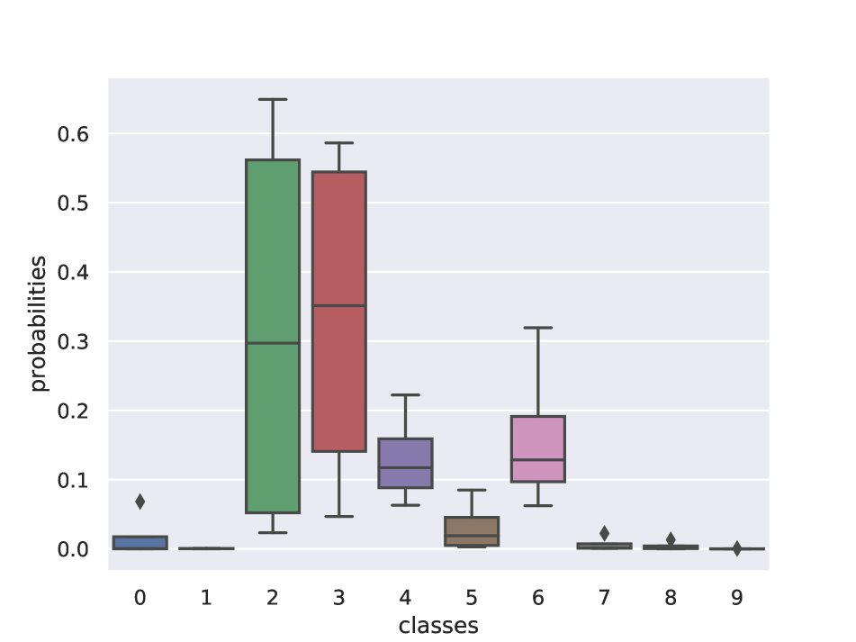
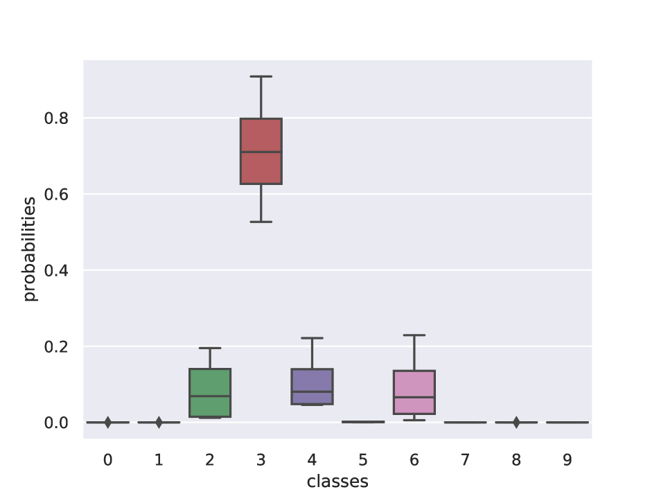
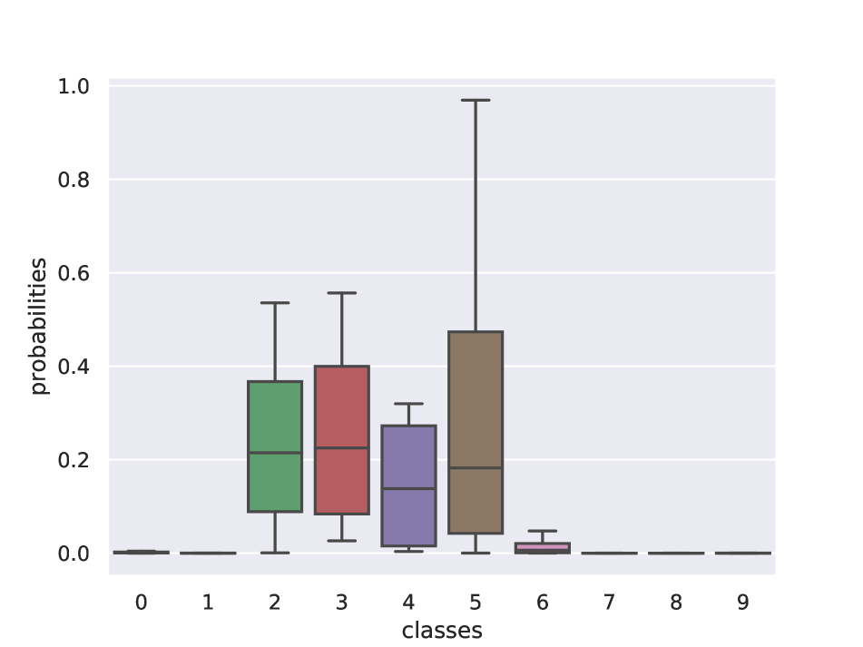
Figure 4: Diversity of predictions of different ensemble methods. Col. $1$: in top-down order images from the test set of CIFAR-10, CIFAR-10-C, and SVHN; Col. $2{-}4$: outputs of different sub-models of the three ensemble techniques: LP-BNN, BE [70], and DE [39]. For all methods we set the number of models to $J{=}4$.

4 Related work

Bayesian Deep Learning.   Bayesian approaches and neural networks have a long joint history [43, 44, 52]. Early approaches relied on Markov chain Monte Carlo variants for inference on BNNs, which was later replaced by variational inference (VI) [33] in the context of deeper networks. Most of the modern approaches make use of VI with the mean-field approximation [27, 19, 6, 26, 17, 51] which conveniently makes posterior inference tractable. However this limits the expressivity of the posterior [44, 12]. This drawback became subject of multiple attempts for structured-covariance approximations using matrix variate Gaussian priors [42, 65] or natural gradients [76, 51]. However they further increase memory and time complexity over the original mean-field approximation. Recent methods proposed more simplistic BNNs by performing inference with structured priors only over the first and last layer [56] or just the last layer [61, 54]. Full covariance can be computed for shallow networks thanks to a meta-prior in a low-dimensional space where the VI can be performed [35, 34]. Most BNNs are still challenging to train, underfit and are difficult to scale to big DNNs [54, 10], while the issue of finding a proper prior is still open [71, 14]. Our approach builds upon the low dimensional fast weights from BE and on the stability of the VAEs, foregoing many of the shortcomings of BNN training.

Ensemble Approaches.   Ensembles mimick and attain, to some extent, properties of BNNs [13]. Deep Ensembles [39] train multiple DNNs with different random initializations leading to excellent uncertainty quantification scores. The major inherent drawback in terms of computational and memory overhead has been subsequently addressed through multi-head networks [40], snapshot-ensembles from intermediate training checkpoints [29, 18], efficient computation of the posterior distribution from weight trajectories during training [45, 15], use of multiple Dropout masks at test time [17], multiple random perturbations to the weights of a pre-trained network [15, 50, 3], multiple perturbation of the input image [2], multiple low-rank weights tied to a backbone network [70], simultaneous processing of multiple images by the same DNN [21]. Most approaches still have a significant computational overhead for training or for prediction, while struggling with diversity [13].

Dirichlet Networks (DNs).   DNs [47, 48, 63, 7, 66] bring a promising line of approaches that estimate uncertainty from a single network by parameterizing a Dirichlet distribution over its predictions. However, most of these methods [47, 48] use OOD samples during training, which may be unrealistic in many applications [7], or do not scale to bigger DNNs [32].DNs have been developed only for classification tasks and extending them to regression requires further adjustments [46], unlike LP-BNN that can be equally used for classification and regression.

5 Experiments and results

5.1 Implementation details

We evaluate the performance of LP-BNN in assessing the uncertainty of its predictions. For our benchmark, we evaluate LP-BNN on different scenarios against several strong baselines with different advantages in terms of performance, training or runtime: BE [70], DE [39], Maximum Class Probability (MCP) [25], MC Dropout [17], TRADI  [15], EDL [63], DUQ [67], and MIMO [21].

First, we evaluate the predictive performance in terms of accuracy for image classification and mIoU [11] for semantic segmentation, respectively. Secondly, we evaluate the quality of the confidence scores provided by the DNNs by means of Expected Calibration Error (ECE) [20]. For ECE we use $M$-bin histograms of confidence scores and accuracy, and compute the average of $M$ bin-to-bin differences between the two histograms. Similarly to [20] we set $M=15$. To evaluate the robustness to dataset shift via corrupted images, we first train the DNNs on CIFAR-10 [38] or CIFAR-100 [38] and then test on the corrupted versions of these datasets [24]. The corruptions include different types of noise, blurring, and some other transformations that alter the quality of the images. For this scenario, similarly to [69], we use as evaluation measures the Corrupted Accuracy (cA) and Corrupted Expected Calibration Error (cE), that offer a better understanding of the behavior of our DNN when facing shift of data distribution and aleatoric uncertainty.

In order to evaluate the epistemic uncertainty, we propose to assess the OOD detection performance. This scenario typically consists in training a DNN over a dataset following a given distribution, and testing it on data coming from this distribution and data from another distribution , not seen during training. We quantify the confidence of the DNN predictions in this setting through their prediction scores, i.e., output softmax values. We use the same indicators of the accuracy of detecting OOD data as in [25]: AUC, AUPR, and the FPR-95%-TPR. These indicators measure whether the DNN model lacks knowledge regarding some specific data and how reliable are its predictions.

	CIFAR-10							CIFAR-100
Method	Acc $\uparrow$	AUC $\uparrow$	AUPR $\uparrow$	FPR-95-TPR $\downarrow$	ECE $\downarrow$	cA $\uparrow$	cE $\downarrow$	Acc $\uparrow$	ECE $\downarrow$	cA $\uparrow$	cE $\downarrow$
MCP + cutout [25]	96.33	0.9600	0.9767	0.115	0.0207	32.98	0.6167	80.19	0.1228	19.33	0.7844
MC dropout [17]	95.95	0.9126	0.9511	0.282	0.0172	32.32	0.6673	75.40	0.0694	19.33	0.5830
MC dropout +cutout [17]	96.50	0.9273	0.9603	0.242	0.0117	32.35	0.6403	77.92	0.0672	27.66	0.5909
DUQ [67]†	87.48	0.7083	0.8114	0.698	0.3983	64.89	0.2542	-	-	-	-
DUQ Resnet18 [67]‡	93.36	0.8994	0.9213	0.1964	0.0131	69.01	0.5059	-	-	-	-
EDL [63]†	85.73	0.9002	0.9198	0.247	0.0904	59.54	0.3412	-	-	-	-
MIMO [21]	94.96	0.9387	0.9648	0.175	0.0300	69.99	0.1846	0.7869	0.1018	0.4735	0.2832
Deep Ensembles + cutout [39]	96.74	0.9803	0.9896	0.071	0.0093	68.75	0.1414	83.01	0.0673	47.35	0.2023
BatchEnsembles + cutout [70]	96.48	0.9540	0.9731	0.132	0.0167	71.67	0.1928	81.27	0.0912	47.44	0.2909
LP-BNN (ours) + cutout	95.02	0.9691	0.9836	0.103	0.0094	69.51	0.1197	79.3	0.0702	48.40	0.2224

Table 1: Comparative results for image classification tasks. We evaluate on CIFAR-10 and CIFAR-100 for the tasks: in-domain classification, out-of-distribution detection with SVHN (CIFAR-10 only), robustness to distribution shift (CIFAR-10-C, CIFAR-100-C). We run all methods ourselves in similar settings using publicly available code for related methods. Results are averaged over three seeds. ^†: We did not manage to scale these methods to WRN-28-10 on CIFAR-100. A similar finding for EDL was reported in  [32]. ^‡ DUQ does not scale on CIFAR-100 and it does not perfectly scale to WRN-28-10 on CIFAR-10 so we train it with Resnet 18 [22] architecture like in the original paper.

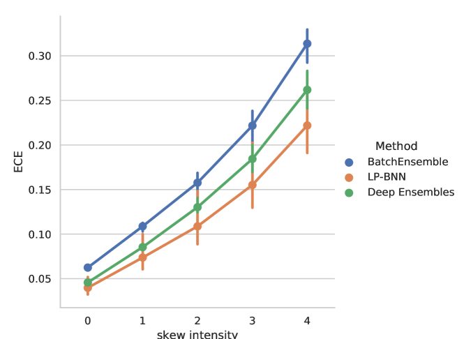
Figure 5: Calibration at different levels of corruption. We report ECE scores for LP-BNN, BE [70], and DE [39] on CIFAR-10-C.

5.2 Image classification with CIFAR-10/100 [38]

Protocol. Here we train on CIFAR-10 [38] composed of 10 classes. For CIFAR-10 we consider as OOD the SVHN dataset [53]. Since SVHN is a color image dataset of digits, it guarantees that the OOD data comes from a distribution different from those of CIFAR-10. We use WRN-28-10 [75] for all methods, a popular architecture for this dataset, and evaluate on CIFAR-10-C [24]. For CIFAR-100 [38] we use again WRN-28-10 and evaluate on the test sets of CIFAR-100 and CIFAR-100-C [24]. Note that for all DNNs, even for DE, we average results over three random seeds for statistical relevance. We use cutout [9] as data augmentation, as commonly used for these datasets. Please find in the supplementary the hyperparameters for this experiment.

Discussion. We illustrate results for this experiment in Table 3. We notice that DE with cutout outperforms other methods on most of the metrics except ECE, cA, and cE on CIFAR-10, and cA on CIFAR-100, where LP-BNN  achieves state of the art results. This means that LP-BNN  is competitive for aleatoric uncertainty estimation. In fact, ECE is calculated on the test set of CIFAR-10 and CIFAR-100, so it mostly measures the reliability of the confidence score in the training distribution. cA and cE are evaluated on corrupted versions of CIFAR-10 and CIFAR-100, which amounts to quantifying the aleatoric uncertainty. We can see that for this kind of uncertainty, LP-BNN  achieves state of the art performance. On the other hand, for epistemic uncertainty, we can see that DE always attain best results. Overall, our LP-BNN  is more computationally efficient while providing better results for the aleatoric uncertainty. Computation wise, DE takes $52$ hours to train on CIFAR-10, while LP-BNN needs 2 times less, $26$ hours and $30$ minutes. In Figure 5 and Table S6, we observe that our method exhibits top ECE score on CIFAR-10-C, as well as for the stronger corruptions.

		Vanilla	BatchEnsemble	Deep Ensembles	TRADI	LP-BNN
Training	Time (s)	1,506	1,983	6,026	1,782	1,999
	for 1 epochs	1	$\times$1.31	$\times$4.0	$\times$1.18	$\times$1.33
	Memory (MiB)	8,848	9,884	35,392	9,040	9,888
		1	$\times$1.11	$\times$4.0	$\times$1.02	$\times$1.11
Testing	Time (s)	0.21	0.56	0.84	0.84	0.57
	on 1 image	1	$\times$2.67	$\times$4.0	$\times$4.0	$\times$2.71
	Memory (MiB)	1,884	4,114	7,536	7,536	4,114
		1	$\times$2.18	$\times$4.0	$\times$4.0	$\times$2.18

Table 2: Runtime and memory analysis. Numbers correspond to StreetHazards images processed with DeepLabv3+ ResNet-50 with PyTorch on a PC: Intel Core i9-9820X and $1\times$ GeForce RTX 2080Ti. Colored numbers are relative to vanilla approach. Mini-batch size for training is $4$ and for testing $1$.

5.3 Semantic segmentation

Next, we evaluate semantic segmentation, a task of interest for autonomous driving, where high capacity DNNs are used for processing high resolution images with complex urban scenery with strong class imbalance.

StreetHazards [23]. StreetHazards is a large-scale dataset that consists of different sets of synthetic images of street scenes. More precisely, this dataset is composed of $5,125$ images for training and $1,500$ test images. The training dataset contains pixel-wise annotations for $13$ classes. The test dataset comprises $13$ training classes and $250$ OOD classes, unseen in the training set, making it possible to test the robustness of the algorithm when facing a diversity of possible scenarios. For this experiment, we used DeepLabv3+ [8] with a ResNet-50 encoder [22]. Following the implementation in [23], most papers use PSPNet [77] that aggregates predictions over multiple scales, an ensembling that can obfuscate in the evaluation the uncertainty contribution of a method. This can partially explain the excellent performance of MCP on the original settings [23]. We propose using DeepLabv3+ instead, as it enables a clearer evaluation of the predictive uncertainty. We propose two DeepLabv3+ variants as follows. DeepLabv3+ is composed of an encoder network and a decoder network; in the first version, we change the decoder by replacing all the convolutions with our new version of LP-BNN convolutions and leave the encoder unchanged. In the second variant we use weight standardization [57] on the convolutional layers of the decoder, replacing batch normalization [30] in the decoder with group normalization [73], to better balance mini-batch size and ensemble size. We denote the first version LP-BNN and the second one LP-BNN + GN.

Dataset	OOD method	mIoU $\uparrow$	AUC $\uparrow$	AUPR $\uparrow$	FPR-95-TPR $\downarrow$	ECE $\downarrow$
StreetHazards DeepLabv3+ ResNet50	Baseline (MCP) [25]	53.90	0.8660	0.0691	0.3574	0.0652
	TRADI [15]	52.46	0.8739	0.0693	0.3826	0.0633
	Deep Ensembles [39]	55.59	0.8794	0.0832	0.3029	0.0533
	MIMO [21]	55.44	0.8738	0.0690	0.3266	0.0557
	BatchEnsemble [70]	56.16	0.8817	0.0759	0.3285	0.0609
	LP-BNN (ours)	54.50	0.8833	0.0718	0.3261	0.0520
	LP-BNN + GN (ours)	56.12	0.8908	0.0742	0.2999	0.0593
BDD-Anomaly DeepLabv3+ ResNet50	Baseline (MCP) [25]	47.63	0.8515	0.0450	0.2878	0.1768
	TRADI [15]	44.26	0.8480	0.0454	0.3687	0.1661
	Deep Ensembles [39]	51.07	0.8480	0.0524	0.2855	0.1419
	MIMO [21]	47.20	0.8438	0.0432	0.3524	0.1633
	BatchEnsemble [70]	48.09	0.8427	0.0449	0.3017	0.1690
	LP-BNN (ours)	49.01	0.8532	0.0452	0.2947	0.1716
	LP-BNN + GN (ours)	47.15	0.8553	0.0577	0.2866	0.1623

Table 3: Comparative results on the OOD task for semantic segmentation. We run all methods ourselves in similar settings using publicly available code for related methods. Results are averaged over three seeds.

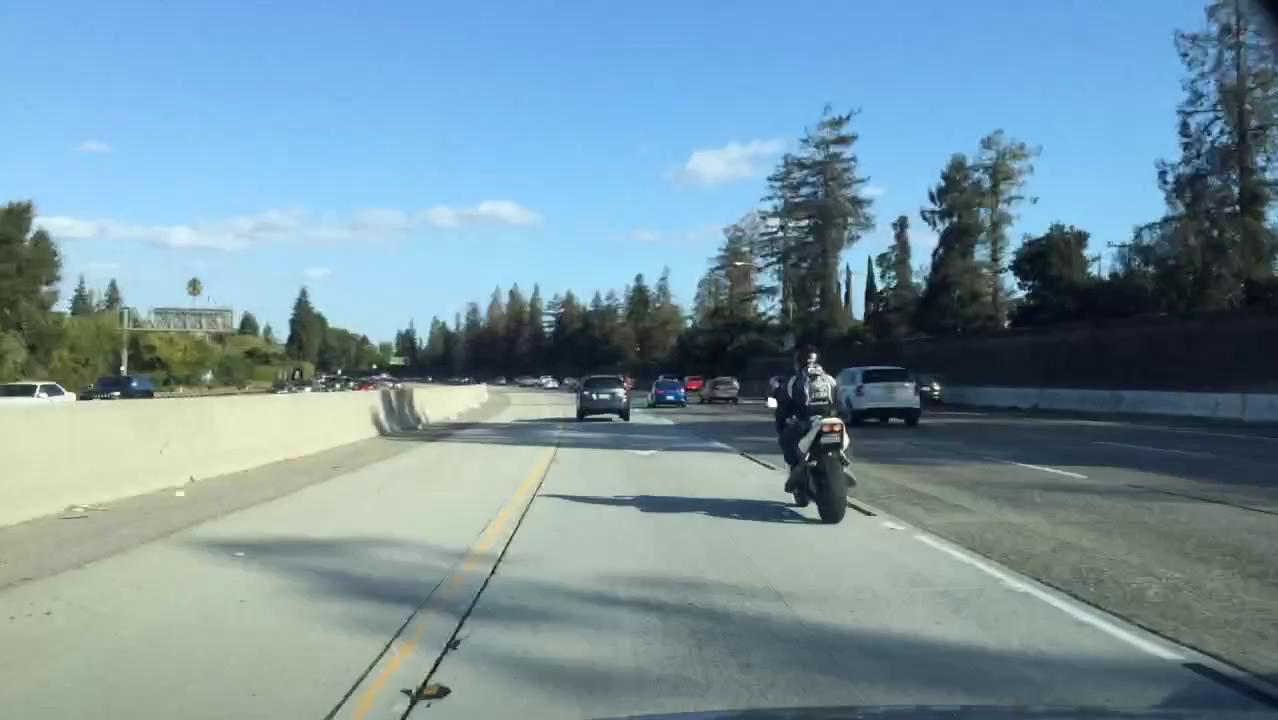
Input image

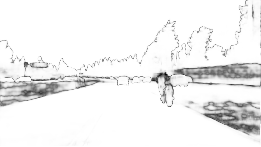
MCP

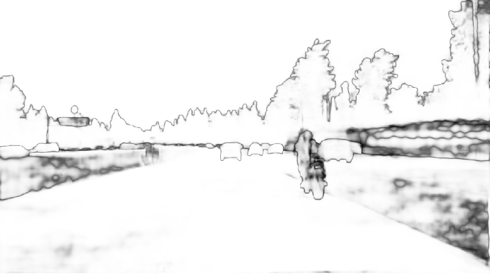
BE

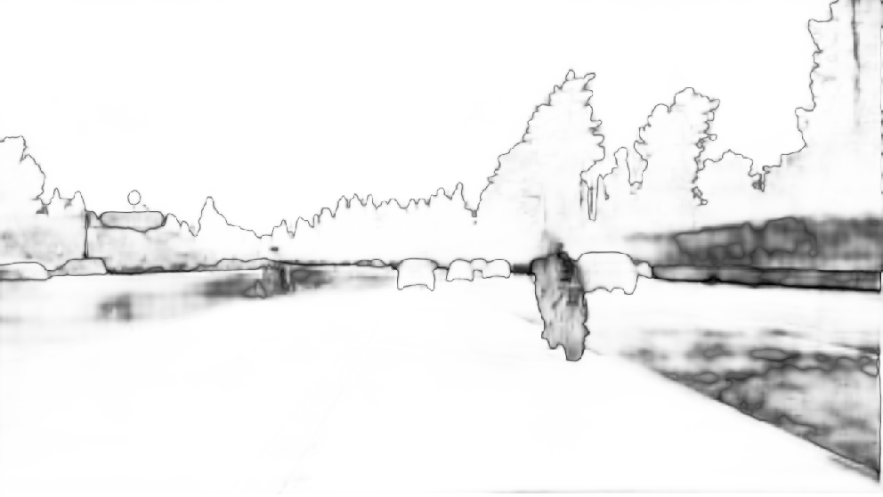
LP-BNN

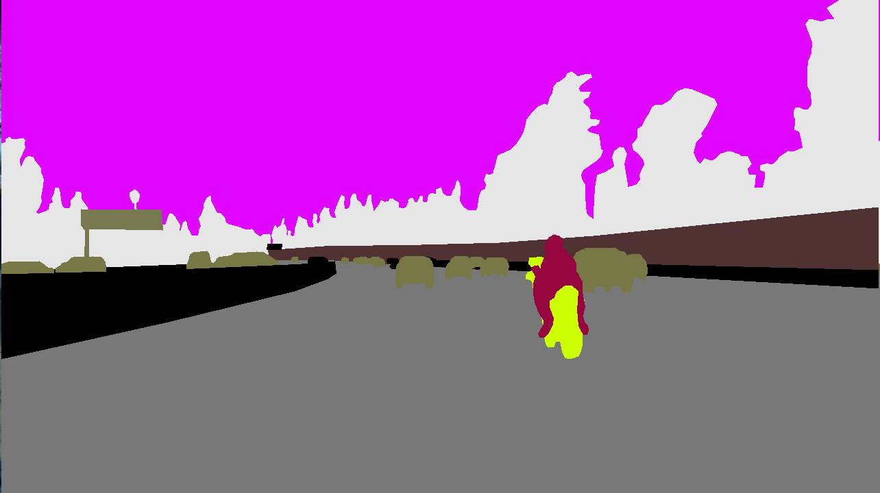
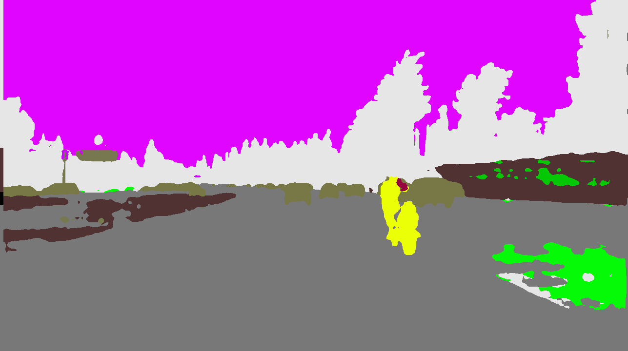
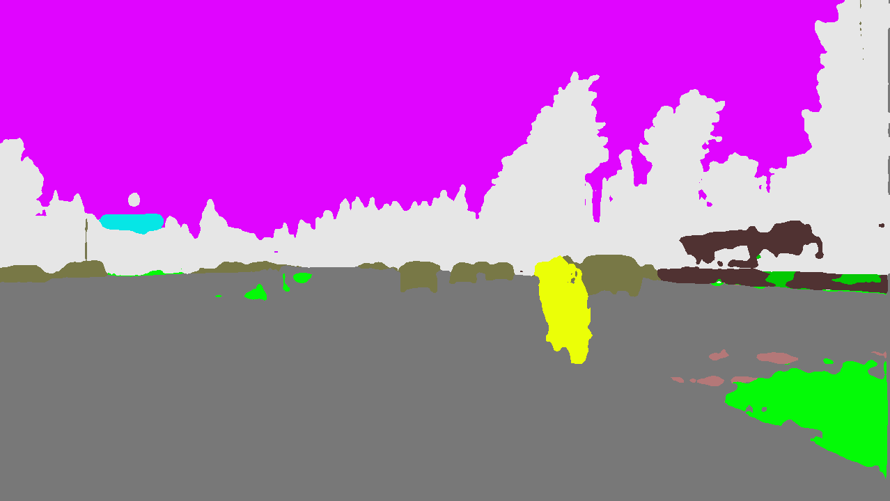
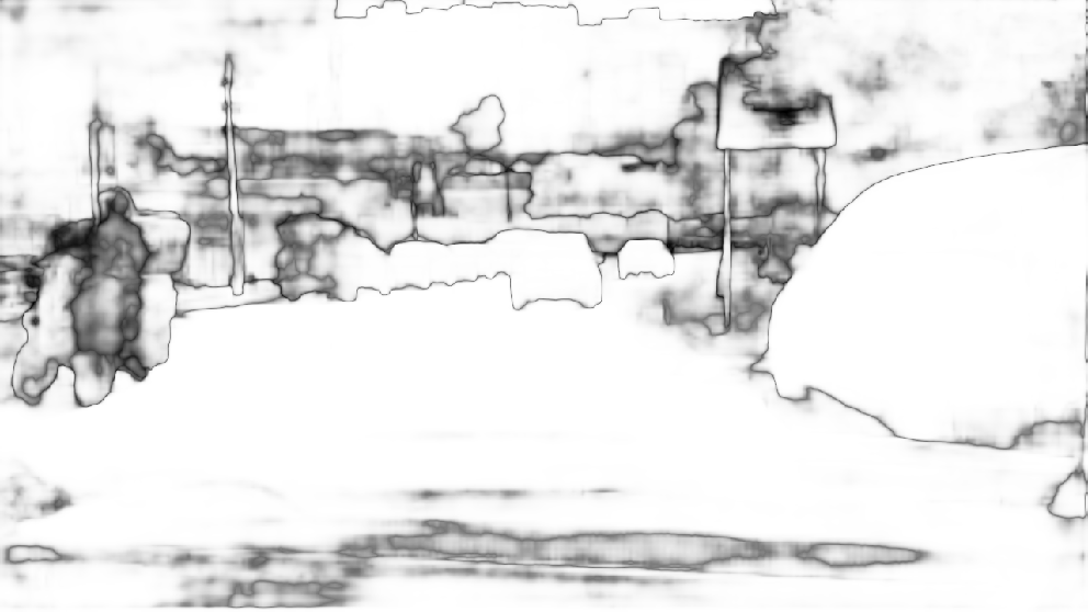
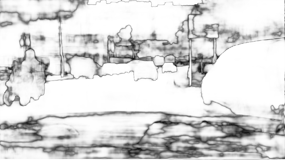
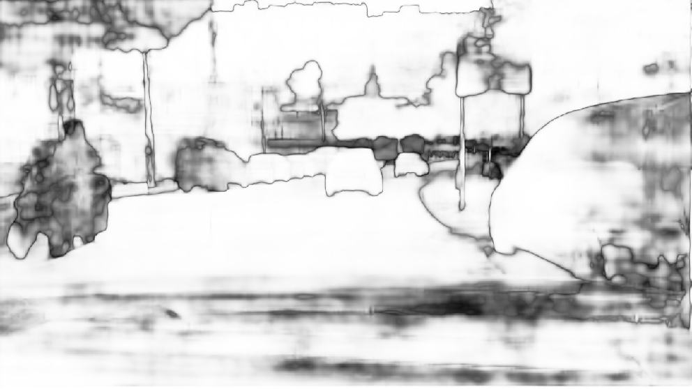
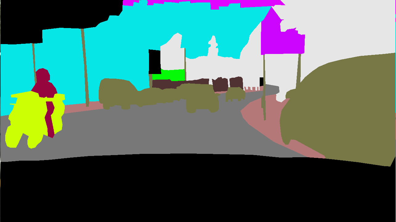
Figure 6: Visual assessment on two BDD-Anomaly test images containing a motorcycle (OOD class). For each image: on the first row, input image and confidence maps from MCP [25], BE [70], and LP-BNN; on the second row, ground-truth segmentation and segmentation maps from MCP, BE, and LP-BNN. LP-BNN is less confident on the OOD objects.

BDD-Anomaly [23]. BDD-Anomaly is a subset of the BDD100K dataset [74], composed of $6,688$ street scenes for training and $361$ for the test set. The training set contains pixel-level annotations for $17$ classes, and the test dataset is composed of the $17$ training classes and $2$ OOD classes: motor-cycle and train. For this experiment, we use DeepLabv3+ [8] with the experimental protocol from [23]. As previously we use ResNet50 encoder [22]. For this experiment, we use the LP-BNN and LP-BNN + GN variants.

Discussion. We emphasize that the semantic segmentation is more challenging than the CIFAR classification since images are bigger and their content is more complex. The larger input size constrains to use smaller mini-batches. This is crucial since the fast weights of the ensemble layers are trained just on one mini-batch slice. In this experiment, we could use mini-batches of size $4$ and train the fast weights on slices of size $1$. Yet, despite these computational difficulties, with our technique, we achieve state-of-the-art results for most metrics. We can see in Table 3 that our strategies achieve state-of-the-art performance in detecting OOD data and are well calibrated. We can also see in Figure 6, where the OOD class is the motorcycle, that our DNN is less confident on this class. Hence LP-BNN allows us to have a more reliable DNN which is essential for real-world applications.

Table 2 shows the computational cost of LP-BNN and related methods. For training, LP-BNN takes only $\times 1.33$ more time than a vanilla approach, in contrast to DE that take much longer, while their performances are equivalent in most cases. In the same time, LP-BNN enables implicit modeling of weight correlations at every layer with limited overhead as it does not explicitly computes the covariances. To the best of our knowledge, LP-BNN is the first approach with the posterior distribution computed with variational inference successfully trained and applied for semantic segmentation.

6 Conclusion

We propose a new BNN framework able to quantify uncertainty in the context of deep learning. Owing to each layer of the network being tied to and regularized by a VAE, LP-BNNs are stable, efficient, and therefore easy to train compared to existing BNN models. The extensive empirical comparisons on multiple tasks show that LP-BNNs reach state-of-the-art levels with substantially lower computational cost. We hope that our work will open new research paths on effective training of BNNs. In the future we intend to explore new strategies for plugging more sophisticated VAEs in our models along with more in-depth theoretical studies.

A Discussion

A.1 Covariance Priors of Bayesian Neural Network

We consider a data sample $(\mathbf{x},y)$, with $\mathbf{x}\in^{d}$ and $y\in$. We process the input data $\mathbf{x}$ with a MLP network $f_{\Theta}(\cdot)$ with parameters $\Theta$ composed of one hidden layer of $h$ neurons. We detail the composing operations of the function $f_{\Theta}(\cdot)$ associated to this network: $f_{\Theta}(x)=W_{2}^{\top}\sigma(W_{1}^{\top}\mathbf{x})$, where $\sigma(\cdot)$ is an element-wise activation function. For simplicity, we ignore the biases in this example. $W_{1}\in^{d\times h}$ is the weight matrix associated with the first fully connected layer and $W_{2}\in^{h\times 1}$ the weights of the second layer. In BNNs, $W_{1}$ and $W_{2}$ represent random variables, while for classic DNNs, they are simply singular realizations of the distribution sought by BNN inference. Most works exploiting in some way the statistics of the network parameters assume, for tractability reasons, that all weights of $W_{1}$ and $W_{2}$ follow independent Gaussian distributions. Hence this will lead to the following covariance matrix for $W_{1}$:

$$\begin{pmatrix}\mbox{var}(W_{1}[1,1])&0&0&\ldots&0\\ 0&\mbox{var}(W_{1}[2,1])&0&\ldots&0\\ \vdots&\ddots&\ddots&\ddots&\vdots\\ 0&0&0&\ldots&\mbox{var}(W_{1}[{\color[rgb]{0,0,0}d,h}])\\ \end{pmatrix}$$

where $\mbox{var}(W_{1}[i,j])$ is the variance of the coefficient $[i,j]$ of matrix $W_{1}$. Similarly, for $W_{2}$ we will have a diagonal matrix.

Now, let us assume that $W_{1}$ and $W_{2}$ have a latent representation $Z_{1}{=}\big{[}Z_{1}[1],Z_{1}[2],Z_{1}[3]\big{]}\in^{3}$ and $Z_{2}{=}\big{[}Z_{2}[1],Z_{2}[2],Z_{3}[3]\big{]}\in^{3}$, respectively, such that for every coefficient $[i,j]$ of $W_{1}$ and $W_{2}$ there exist real weights $\{\alpha^{[i,j]}_{1}[k]\}_{k=1}^{3}$ and $\{\alpha^{[i,j]}_{2}[k]\}_{k=1}^{3}$ such that: $W_{1}[i,j]{=}\sum_{k=1}^{3}\alpha_{1}^{[i,j]}[k]Z_{1}[k]$ and $W_{2}{=}\sum_{k=1}^{3}\alpha^{[i,j]}_{2}[k]Z_{2}[k]$, respectively. In the case of LP-BNN, we consider that each coefficient of $Z_{1}$ and $Z_{2}$ represent an independent random variable. Thus, in contrast to approaches based on the mean-field approximation directly on the weights of the DNN, we can have for each layer a non-diagonal covariance matrix with the following variance and covariance terms for $W_{1}$:

$$\mbox{var}(W_{1}[i,j])=\sum_{k=1}^{3}(\alpha^{[i,j]}_{1}[k])^{2}\mbox{var}(Z_{1}[k])$$ (S1)

$$\mbox{cov}(W_{1}[i,j],W_{1}[i^{\prime},j^{\prime}])=\sum_{k=1}^{3}\alpha^{[i,j]}_{1}[k]\alpha^{[i^{\prime},j^{\prime}]}_{1}[k]\mbox{var}(Z_{1}[k])$$ (S2)

This allows us to leverage the lower-dimensional parameters of the distributions of $Z_{1}$ and $Z_{2}$ for estimating the higher-dimensional distributions of $W_{1}$ and $W_{2}$. In this manner, in LP-BNN we model an implicit covariance of weights at each layer.

We note that several approaches for modeling correlation between weights have been proposed under certain settings and assumptions. For instance, Karaletesos and Bui [34] model correlations between weights within a layer and across layers thanks to a Gaussian process-based approach working in the function space via hierarchical priors instead of directly on the weights. Albeit elegant, this approach is still limited to relatively shallow MLPs (e.g., one hidden layer with 100 units [34]) and cannot scale up yet to deep architectures considered in this work (e.g., ResNet-50). Other approaches [42, 65] model layer-level weight correlations through Matrix Variate Gaussian (MVG) prior distributions, increasing the expressiveness of the inferred posterior distribution at the cost of further increasing the computational complexity w.r.t. mean-field approximated BNNs [6, 19]. In contrast, LP-BNN does not explicitly model the covariance by conveniently leveraging fully connected layers to project weights in a low-dimensional latent space and performing the inference of the posterior distribution there. This strategy leads to a lighter BNN that is competitive in terms of computation and performance for complex computer vision tasks.

A.2 The utility of Rank-1 perturbations

One could ask why using the Rank-1 perturbation formalism from BE [70], instead of simply feeding the weights of a layer to the VAE to infer the latent distribution. Rank-1 perturbations significantly reduce the number of weights upon which we train the VAE, due to the decomposition of the fast weights into $\mathbf{r}$ and $\mathbf{s}$. This further allows us to consider multiple such weights, $J$, at each forward pass enabling faster training of the VAE as its training samples are more numerous and more diverse.

Next, we establish connections between the cardinality $J$ of the ensemble and the posterior covariance matrix. The mechanism of placing a prior distribution over the latent space enables an implicit modeling of correlations between weights in their original space. This is a desirable property due to its superior expressiveness [12, 34] but which can be otherwise computationally intractable or difficult to approximate. The covariance matrix of our prior in the original weight space is a Rank-1 matrix. Thanks to the Eckart-Young theorem (Theorem 5.1 in [68]), we can quantify the error of approximating the covariance by a Rank-1 matrix, based on the second up to the last singular values.

Let us denote by $\Theta_{1},\ldots,\Theta_{J}$ the $J$ weights trained by our algorithm, $\Theta_{\text{avg}}=\frac{1}{J}\sum_{j=1}^{J}\Theta_{j}$ and $\Delta_{j}=\Theta_{j}-\Theta_{\text{avg}}$. The differences and the sum in the previous equations are calculated element-wise on all the weights of the DNNs. Then, for each new data sample $\mathbf{x}$, the prediction of the DNN $f_{\Theta_{\text{avg}}}(\cdot)$ is equivalent to the average of the DNNs $f_{\Theta_{j}}(\cdot)$ applied on $\mathbf{x}$ :

$$\frac{1}{J}\sum_{j=1}^{J}f_{\Theta_{j}}(\mathbf{x})=f_{\Theta_{\text{avg}}}(\mathbf{x})+\mathcal{O}\left(\|\Delta\|^{2}\right)$$ (S3)

with $\|\Delta\|=\max_{j}\|\Delta_{j}\|$. The $L_{2}$ norm is computed over all weights. We refer the reader to the proof in §3.5 of [31]. It follows that in fact we do not learn a Rank-1 matrix, but an up to Rank-$J$ covariance matrix, if all the $\mathbf{s}_{j}$ $\mathbf{r}_{j}$ are independent. Hence the choice of $J$ acts as an approximation factor of the covariance matrix. Wen et al. [70] tested different values of $J$ and found that $J=4$ was the best compromise, which we also use here.

A.3 Computational complexity

Recent works [13, 72] studied the weight modes computed by Deep Ensembles under a BNN lens, yet these approaches are computationally prohibitive at the scale required for practical computer vision tasks. Recently, Dusenberry et al. [10] proposed a more scalable approach for BNNs, which can still be subject to high instabilities as the ELBO loss is applied over a high-dimensional parameter space, all BatchEnsemble parameters. Increased stability can be achieved by leveraging large mini-batches that bring more robust feature and gradient statistics, at significantly higher computational cost (large virtual mini-batches are obtained through distributed training over multiple TPUs). In comparison, our approach has a smaller memory overhead since we encode $\mathbf{r}_{j}$ in a lower dimensional space (we found empirically that a latent space of size only $32$ provides an appealing compromise between accuracy and compactness). The ELBO loss here is applied over this lower-dimensional space which is easier to optimize. The only additional cost in terms of parameters and memory used w.r.t. BE is related to the compact VAEs associated with each layer.

In addition to the lower number of parameters, LP-BNN training is more stable than for Rank-1 BNN [10] due to the reconstruction term $\|\mathbf{r}_{j}-\hat{\mathbf{r}}_{j}\|^{2}_{2}$ which regularizes the $\mathcal{L}_{\scriptscriptstyle\text{LP-BNN}}$ loss in Eq. (7) of the main paper by controlling the variances of the sampled weights. In practice, to train BNNs successfully, a range of carefully crafted heuristics are necessary, e.g., clipping, initialization from truncated Normal distributions, extra weight regularization to stabilize training [10]. For LP-BNN, training is overall straightforward even on complex and deep models, e.g., DeepLabV3+, thanks to the VAE module that is stable and trains faster.

Learning Rate	0.2	0.1	0.05	0.01	0.005
BNN accuracy	22.48	44.60	49.83	48.70	56.69
BNN epoch div	3	25	65	None	None
LP-BNN accuracy	20.02	55.04	59.68	63.73	64.41
LP-BNN epoch div	3	None	None	None	None

Table S1: Stability analysis of BNNs. Stability experiment with LeNet 5 architecture and 80 epochs on CIFAR-10. On the epoch divergence row, None means that the DNN does not diverge.

A.4 Stability of Bayesian Neural Networks

In this section, we experiment on CIFAR-10 to evaluate the stability of LP-BNN versus a classic BNN. For this experiment, we use the LeNet-5 architecture and choose a weight decay of $1e-4$ along with a mini-batch size of $128$. Our goal is to see whether both techniques are stable when we vary the learning rate. Both DNNs were trained under the exact same conditions for $80$ epochs. In Table S1, we present two metrics for both DNNs. The first metric is the accuracy. The second metric is the epoch during which the training loss of the DNN explodes, i.e., is equal to infinity. This phenomenon may occur if the DNN is highly unstable to train. We argue that LP-BNN is visibly more stable and standard BNNs during training. We can see from Table S1 that LP-BNN is more stable than the standard BNN as it does not diverge for a wide range of learning rates. Moreover, its accuracy is higher than that of a standard BNN implemented on the same architecture, a property that we attribute to the VAE regularization.

A.5 LP-BNN diversity

	ratio errors $\uparrow$	Q-statistic $\downarrow$	correlation coefficient $\downarrow$
DE	0.9825	0.9877	0.6583
BE	0.5915	0.9946	0.7634
LP-BNN	0.8390	0.9842	0.6601

Table S2: Comparative results of diversity scores for image classification on the CIFAR-10 dataset.

	ratio errors $\uparrow$	Q-statistic $\downarrow$	correlation coefficient $\downarrow$
DE	0.4193	0.9690	0.7568
BE	0.2722	0.9874	0.8352
LP-BNN	0.4476	0.9595	0.7332

Table S3: Comparative results of diversity scores for image classification on the CIFAR-10-C dataset.

At test-time, BNNs and DE aggregate the different predictions. For BNNs, these predictions come from the different realizations of the posterior distribution, while, for the DE, these predictions are provided by several DNNs trained in parallel. As proved in [13, 59], the diversity among these different predictions is key to quantify the uncertainty of a DNN. Indeed, we want the different DNN predictions to have a high variance when the model is not accurate. Figure S1 highlights this desirable property of high variance on out-of-distribution samples exhibited by LP-BNN. Also, as in [59], we evaluate the ratio-error introduced in [1]. The ratio-error between two classifiers is the number of data samples on which only one classifier is wrong divided by the number of samples on which they are both wrong. A higher value means that the two classifiers are less likely to make the same errors. We also evaluated the Q-statistics [1], which measures the diversity between two classifiers. The value of the Q-statistics is between $-1$ and $1$ and is defined as:

$$Q=\frac{N_{11}N_{00}-N_{10}N_{01}}{N_{11}N_{00}+N_{10}N_{01}}$$ (S4)

where $N_{11}$ and $N_{00}$ are the numbers of data on which both classifiers are correct and incorrect, respectively. $N_{10}$ and $N_{01}$ are the number of data where just one of the two classifiers is wrong. If the two classifiers are always wrong or right for all data, then $N_{10}{=}N_{01}{=}0$ and $Q{=}1$, while if both classifiers always make errors on different inputs, then $Q{=}-1$. The maximum diversity comes when $Q$ is minimum.

Finally, we evaluated the correlation coefficient [1], which assesses the correlation between the error vectors of the two classifiers. Tables S2 and S3 illustrate that, for the normal case (CIFAR-10), LP-BNN displays similar diversity with DE, while in the corrupted case (CIFAR-10-C) LP-BNN achieves better diversity scores. We conclude that in terms of diversity metrics, LP-BNN has indeed the behavior that one would expect for uncertainty quantification purposes.

Input
LP-BNN
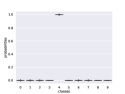
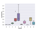
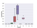
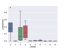
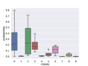
BE
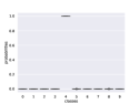
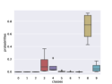
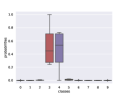
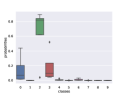
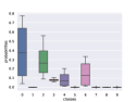
DE

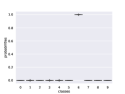
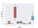
Figure S1: Diversity of predictions of different ensemble methods. The first row contains in order two images from the test set of CIFAR-10, of CIFAR-10-C and of SVHN, respectively. The next three rows represent the corresponding outputs of the different sub models for the three ensembling algorithms being considered: LP-BNN, BatchEnsemble and Deep Ensembles.

B Implementation details

For our implementation, we use PyTorch [55] and will release the code after the review in order to facilitate reproducibility and further progress. In the following we share the hyper-parameters for our experiments on image classification and semantic segmentation.

B.1 Semantic segmentation experiments

In Table S4, we summarize the hyper-parameters used in the StreetHazards [23] and BDD-Anomaly [23] experiments.

Hyper-parameter	StreetHazards	BDD-Anomaly
Ensemble size $J$	4	4
learning rate	0.1	0.1
batch size	4	4
number of train epochs	25	25
weight decay for $\theta^{\text{slow}}$ weights	0.0001	0.0001
weight decay for $\theta^{\text{fast}}$ weights	0.0	0.0
cutout	True	True
SyncEnsemble BN	False	False
Group Normalisation	True	True
Size of the latent space $\mathbf{z}$	32	32

Table S4: Hyper-parameter configuration used in the semantic segmentation experiments (§5.3).

Hyper-parameter	CIFAR-10	CIFAR-100
Ensemble size $J$	4	4
initial learning rate	0.1	0.1
batch size	128	128
lr decay ratio	0.1	0.1
lr decay epochs	[80, 160, 200]	[80, 160, 200]
number of train epochs	250	250
weight decay for $\theta^{\text{slow}}$ weights	0.0001	0.0001
weight decay for $\theta^{\text{fast}}$ weights	0.0	0.0
cutout	True	True
SyncEnsemble BN	False	False
Size of the latent space $\mathbf{z}$	32	32

Table S5: Hyper-parameter configuration used in the classification experiments (§5.2).

B.2 Image classification experiments

In Table S5, we summarize the hyper-parameters used in the CIFAR-10 [38] and CIFAR-100 [38] experiments.

C Notations

In Table S6, we summarize the main notations used in the paper. Table S6 should facilitate the understanding of Section 2 (the preliminaries) and Section 3 (the presentation of our approach) of the main paper.

Notations	Meaning
$\mathcal{D}=\{(\mathbf{x}_{i},y_{i})\}_{i=1}^{n}$	the set of $n$ data samples and the corresponding labels
$\Theta$	the set of weights of a DNN
$P(\Theta)$	the prior distribution over the weights of a DNN
$Q_{\nu}(\Theta)$	the variational prior distribution over the weights of a DNN used in standard BNNs [6]
$\nu$	the parameters of the variational prior distribution over the weights of a DNN used in standard BNNs [6]
$P(y_{i}\mid\mathbf{x}_{i},\Theta)$	the likelihood that DNN outputs $y_{i}$ following a prediction over input image $\mathbf{x}_{i}$
$J$	the number of ensembling DNNs
$\theta^{\text{slow}}=\{\mathrm{W}_{\scriptstyle\text{share}}\}$	the shared “slow” weights of the network
$\theta^{\text{fast}}=\{\mathrm{W}_{j}\}_{j=1}^{J}=\{(\mathbf{r}_{j},\mathbf{s}_{j})\}_{j=1}^{J}$	the set of individual “fast” weights of BatchEnsemble for ensembling of $J$ networks
$\theta^{\text{fast}}=\{(\hat{\mathbf{r}}_{j},\mathbf{s}_{j})\}_{j=1}^{J}$	the set of fast weights of LP-BNN  for ensembling of $J$ networks.
	$\hat{\mathbf{r}}_{j}$ are sampled from the latent weight space of weights $\mathbf{r}_{j}$.
$\theta^{\text{variational}}=\{(\phi_{j},\bm{\psi}_{j})\}_{j=1}^{J}$	the parameters of the VAE for computing the low dimensional latent distribution of $\mathbf{r}_{j}$
$g^{\scriptstyle\text{enc}}_{\scriptstyle\phi}(\cdot)$	the encoder of the VAE applied on $\mathbf{r}$
$g^{\scriptstyle\text{dec}}_{\scriptstyle\psi}(\cdot)$	the decoder of the VAE for reconstructing $\hat{\mathbf{r}}$ from latent code of $\mathbf{r}$
$Q_{\phi}(\mathbf{z}\mid\mathbf{r})$	the variational distribution over the weights $\mathbf{r}$ to approximate the intractable posterior $P_{\psi}(\mathbf{z}\mid\mathbf{r})$
$(\bm{\mathbf{\mu}}_{j},\bm{\mathbf{\sigma}}_{j})=g^{\scriptstyle\text{enc}}_{\scriptstyle\phi}(\mathbf{r}_{j})$	encoder output that parameterize a multivariate Gaussian with diagonal covariance
$\mathbf{z}_{j}\sim Q_{\phi}(\mathbf{z}\mid\mathbf{r})=\mathcal{N}(\mathbf{z};\bm{\mathbf{\mu}}_{j},\bm{\mathbf{\sigma}}^{2}_{j}\mathbf{I})$	sampling a latent code $\mathbf{z}$ from the latent distribution
$P_{\psi}(\mathbf{z}_{j})=\mathcal{N}(\mathbf{z};0,\mathbf{I})$ with $j\in[1,J]$	the prior distribution on $\mathbf{z}_{j}$
$\hat{\mathbf{r}}_{j}=g^{\scriptstyle\text{dec}}_{\scriptstyle\psi}(\mathbf{z}_{j})$	the reconstruction of $\mathbf{r}_{j}$ from its latent distribution , i.e. the variational fast weights
$\overline{\mathrm{W}}_{j}=\mathrm{W}_{\scriptstyle\text{share}}\odot{\color[rgb]{0,0,0}(\mathbf{r}_{j}\mathbf{s}_{j}^{\top})}$	the weight of a BatchEnsemble network $j$ computed from slow and fast weights
	where $\odot$ is the Hadamard product and $(\mathbf{r}_{j}\mathbf{s}_{j}^{\top})$ the inner product between these two vectors.
$\overline{\mathrm{W}}_{j}=\mathrm{W}_{\scriptstyle\text{share}}\odot{\color[rgb]{0,0,0}(\hat{\mathbf{r}}_{j}\mathbf{s}_{j}^{\top})}$	the weight of LP-BNN  network network $j$ computed from slow and variational fast weights

Table S6: Summary of the main notations of the paper.

References

- [1] Matti Aksela. Comparison of classifier selection methods for improving committee performance. In International Workshop on Multiple Classifier Systems, 2003.
- [2] Arsenii Ashukha, Alexander Lyzhov, Dmitry Molchanov, and Dmitry Vetrov. Pitfalls of in-domain uncertainty estimation and ensembling in deep learning. In ICLR, 2020.
- [3] Andrei Atanov, Arsenii Ashukha, Dmitry Molchanov, Kirill Neklyudov, and Dmitry Vetrov. Uncertainty estimation via stochastic batch normalization. In arXiv, 2018.
- [4] Yoshua Bengio, Ian Goodfellow, and Aaron Courville. Deep learning. MIT press, 2017.
- [5] Umang Bhatt, Yunfeng Zhang, Javier Antorán, Q Vera Liao, Prasanna Sattigeri, Riccardo Fogliato, Gabrielle Gauthier Melançon, Ranganath Krishnan, Jason Stanley, Omesh Tickoo, et al. Uncertainty as a form of transparency: Measuring, communicating, and using uncertainty. In arXiv, 2020.
- [6] Charles Blundell, Julien Cornebise, Koray Kavukcuoglu, and Daan Wierstra. Weight uncertainty in neural networks. In ICML, 2015.
- [7] Bertrand Charpentier, Daniel Zügner, and Stephan Günnemann. Posterior network: Uncertainty estimation without ood samples via density-based pseudo-counts. In NeurIPS, 2020.
- [8] Liang-Chieh Chen, Yukun Zhu, George Papandreou, Florian Schroff, and Hartwig Adam. Encoder-decoder with atrous separable convolution for semantic image segmentation. In ECCV, 2018.
- [9] Terrance DeVries and Graham W Taylor. Improved regularization of convolutional neural networks with cutout. In arXiv, 2017.
- [10] Michael W. Dusenberry, Ghassen Jerfel, Yeming Wen, Yian Ma, Jasper Snoek, Katherine Heller, Balaji Lakshminarayanan, and Dustin Tran. Efficient and scalable bayesian neural nets with rank-1 factors. In ICML, 2020.
- [11] Mark Everingham, SM Ali Eslami, Luc Van Gool, Christopher KI Williams, John Winn, and Andrew Zisserman. The pascal visual object classes challenge: A retrospective. IJCV, 111(1), 2015.
- [12] Andrew YK Foong, David R Burt, Yingzhen Li, and Richard E Turner. On the expressiveness of approximate inference in bayesian neural networks. In NeurIPS, 2020.
- [13] Stanislav Fort, Huiyi Hu, and Balaji Lakshminarayanan. Deep ensembles: A loss landscape perspective. In arXiv, 2019.
- [14] Vincent Fortuin, Adrià Garriga-Alonso, Florian Wenzel, Gunnar Rätsch, Richard Turner, Mark van der Wilk, and Laurence Aitchison. Bayesian neural network priors revisited. In AABI, 2021.
- [15] Gianni Franchi, Andrei Bursuc, Emanuel Aldea, Séverine Dubuisson, and Isabelle Bloch. Tradi: Tracking deep neural network weight distributions. In ECCV, 2020.
- [16] Yarin Gal. Uncertainty in deep learning. PhD Thesis, University of Cambridge, 2016.
- [17] Yarin Gal and Zoubin Ghahramani. Dropout as a bayesian approximation: Representing model uncertainty in deep learning. In ICML, 2016.
- [18] Timur Garipov, Pavel Izmailov, Dmitrii Podoprikhin, Dmitry Vetrov, and Andrew Gordon Wilson. Loss surfaces, mode connectivity, and fast ensembling of dnns. In NeurIPS, 2018.
- [19] Alex Graves. Practical variational inference for neural networks. In NeurIPS, 2011.
- [20] Chuan Guo, Geoff Pleiss, Yu Sun, and Kilian Q Weinberger. On calibration of modern neural networks. In ICML, 2017.
- [21] Marton Havasi, Rodolphe Jenatton, Stanislav Fort, Jeremiah Zhe Liu, Jasper Snoek, Balaji Lakshminarayanan, Andrew M Dai, and Dustin Tran. Training independent subnetworks for robust prediction. In arXiv, 2020.
- [22] Kaiming He, Xiangyu Zhang, Shaoqing Ren, and Jian Sun. Deep residual learning for image recognition. In CVPR, 2016.
- [23] Dan Hendrycks, Steven Basart, Mantas Mazeika, Mohammadreza Mostajabi, Jacob Steinhardt, and Dawn Song. A benchmark for anomaly segmentation. In arXiv, 2019.
- [24] Dan Hendrycks and Thomas Dietterich. Benchmarking neural network robustness to common corruptions and perturbations. In ICLR, 2018.
- [25] Dan Hendrycks and Kevin Gimpel. A baseline for detecting misclassified and out-of-distribution examples in neural networks. In ICLR, 2017.
- [26] José Miguel Hernández-Lobato and Ryan Adams. Probabilistic backpropagation for scalable learning of bayesian neural networks. In ICML, 2015.
- [27] Geoffrey E Hinton and Drew Van Camp. Keeping the neural networks simple by minimizing the description length of the weights. In COLT, 1993.
- [28] Stephen C Hora. Aleatory and epistemic uncertainty in probability elicitation with an example from hazardous waste management. RESS, 54(2-3), 1996.
- [29] Gao Huang, Yixuan Li, Geoff Pleiss, Zhuang Liu, John E Hopcroft, and Kilian Q Weinberger. Snapshot ensembles: Train 1, get m for free. 2017.
- [30] Sergey Ioffe and Christian Szegedy. Batch normalization: Accelerating deep network training by reducing internal covariate shift. In ICML, 2015.
- [31] Pavel Izmailov, Dmitrii Podoprikhin, Timur Garipov, Dmitry Vetrov, and Andrew Gordon Wilson. Averaging weights leads to wider optima and better generalization. In UAI, 2018.
- [32] Taejong Joo, Uijung Chung, and Min-Gwan Seo. Being bayesian about categorical probability. In ICML, 2020.
- [33] Michael I Jordan, Zoubin Ghahramani, Tommi S Jaakkola, and Lawrence K Saul. An introduction to variational methods for graphical models. Machine learning, 37(2), 1999.
- [34] Theofanis Karaletsos and Thang D Bui. Hierarchical gaussian process priors for bayesian neural network weights. In NeurIPS, 2020.
- [35] Theofanis Karaletsos, Peter Dayan, and Zoubin Ghahramani. Probabilistic meta-representations of neural networks. In UAI, 2018.
- [36] Diederik P. Kingma and Max Welling. Auto-encoding variational bayes. In ICLR, 2014.
- [37] Benjamin Kompa, Jasper Snoek, and Andrew L Beam. Second opinion needed: communicating uncertainty in medical machine learning. NPJ Digital Medicine, 4(1), 2021.
- [38] Alex Krizhevsky, Geoffrey Hinton, et al. Learning multiple layers of features from tiny images. Technical report, 2009.
- [39] Balaji Lakshminarayanan, Alexander Pritzel, and Charles Blundell. Simple and scalable predictive uncertainty estimation using deep ensembles. In NeurIPS, 2017.
- [40] Stefan Lee, Senthil Purushwalkam, Michael Cogswell, David Crandall, and Dhruv Batra. Why m heads are better than one: Training a diverse ensemble of deep networks. arXiv preprint arXiv:1511.06314, 2015.
- [41] Chunyuan Li, Heerad Farkhoor, Rosanne Liu, and Jason Yosinski. Measuring the intrinsic dimension of objective landscapes. In ICLR, 2018.
- [42] Christos Louizos and Max Welling. Structured and efficient variational deep learning with matrix gaussian posteriors. In ICML, 2016.
- [43] David JC MacKay. Bayesian methods for adaptive models. PhD thesis, California Institute of Technology, 1992.
- [44] David JC MacKay. A practical bayesian framework for backpropagation networks. Neural computation, 4(3), 1992.
- [45] Wesley J Maddox, Pavel Izmailov, Timur Garipov, Dmitry P Vetrov, and Andrew Gordon Wilson. A simple baseline for bayesian uncertainty in deep learning. In NeurIPS, 2019.
- [46] Andrey Malinin, Sergey Chervontsev, Ivan Provilkov, and Mark Gales. Regression prior networks, 2020.
- [47] Andrey Malinin and Mark Gales. Predictive uncertainty estimation via prior networks. In NeurIPS, 2018.
- [48] Andrey Malinin and Mark Gales. Reverse kl-divergence training of prior networks: Improved uncertainty and adversarial robustness. In NeurIPS, 2019.
- [49] Rowan McAllister, Yarin Gal, Alex Kendall, Mark Van Der Wilk, Amar Shah, Roberto Cipolla, and Adrian Weller. Concrete problems for autonomous vehicle safety: Advantages of bayesian deep learning. IJCAI, 2017.
- [50] Alireza Mehrtash, Purang Abolmaesumi, Polina Golland, Tina Kapur, Demian Wassermann, and William Wells. Pep: Parameter ensembling by perturbation. In NeurIPS, 2020.
- [51] Aaron Mishkin, Frederik Kunstner, Didrik Nielsen, Mark Schmidt, and Mohammad Emtiyaz Khan. Slang: Fast structured covariance approximations for bayesian deep learning with natural gradient. In NeurIPS, 2018.
- [52] Radford M Neal. Bayesian learning for neural networks. PhD thesis, University of Toronto, 1995.
- [53] Yuval Netzer, Tao Wang, Adam Coates, Alessandro Bissacco, Bo Wu, and Andrew Y Ng. Reading digits in natural images with unsupervised feature learning. In NeurIPS, 2011.
- [54] Yaniv Ovadia, Emily Fertig, Jie Ren, Zachary Nado, David Sculley, Sebastian Nowozin, Joshua V Dillon, Balaji Lakshminarayanan, and Jasper Snoek. Can you trust your model’s uncertainty? evaluating predictive uncertainty under dataset shift. In NeurIPS, 2019.
- [55] Adam Paszke, Sam Gross, Francisco Massa, Adam Lerer, James Bradbury, Gregory Chanan, Trevor Killeen, Zeming Lin, Natalia Gimelshein, Luca Antiga, et al. Pytorch: An imperative style, high-performance deep learning library. In NeurIPS, 2019.
- [56] Tim Pearce, Andrew YK Foong, and Alexandra Brintrup. Structured weight priors for convolutional neural networks. In ICMLW, 2020.
- [57] Siyuan Qiao, Huiyu Wang, Chenxi Liu, Wei Shen, and Alan Yuille. Rethinking normalization and elimination singularity in neural networks. In arXiv, 2019.
- [58] Siyuan Qiao, Huiyu Wang, Chenxi Liu, Wei Shen, and Alan Yuille. Weight standardization. In arXiv, 2019.
- [59] Alexandre Rame and Matthieu Cord. Dice: Diversity in deep ensembles via conditional redundancy adversarial estimation. In ICLR, 2021.
- [60] Danilo Jimenez Rezende, Shakir Mohamed, and Daan Wierstra. Stochastic backpropagation and approximate inference in deep generative models. In ICML, 2014.
- [61] Carlos Riquelme, George Tucker, and Jasper Snoek. Deep bayesian bandits showdown: An empirical comparison of bayesian deep networks for thompson sampling. 2018.
- [62] Tim Salimans and Durk P Kingma. Weight normalization: A simple reparameterization to accelerate training of deep neural networks. In NeurIPS, 2016.
- [63] Murat Sensoy, Lance M Kaplan, and Melih Kandemir. Evidential deep learning to quantify classification uncertainty. In NeurIPS, 2018.
- [64] Nitish Srivastava, Geoffrey Hinton, Alex Krizhevsky, Ilya Sutskever, and Ruslan Salakhutdinov. Dropout: A simple way to prevent neural networks from overfitting. JMLR, 15(1), 2014.
- [65] Shengyang Sun, Changyou Chen, and Lawrence Carin. Learning structured weight uncertainty in bayesian neural networks. In AISTATS, 2017.
- [66] Theodoros Tsiligkaridis. Information aware max-norm dirichlet networks for predictive uncertainty estimation. Neural Networks, 135, 2021.
- [67] Joost Van Amersfoort, Lewis Smith, Yee Whye Teh, and Yarin Gal. Uncertainty estimation using a single deep deterministic neural network. In ICML, 2020.
- [68] Jianzhong Wang. Geometric structure of high-dimensional data and dimensionality reduction. Springer, 2012.
- [69] Yeming Wen, Ghassen Jerfel, Rafael Muller, Michael W Dusenberry, Jasper Snoek, Balaji Lakshminarayanan, and Dustin Tran. Improving calibration of batchensemble with data augmentation. In ICMLW, 2020.
- [70] Yeming Wen, Dustin Tran, and Jimmy Ba. Batchensemble: an alternative approach to efficient ensemble and lifelong learning. In ICLR, 2020.
- [71] Florian Wenzel, Kevin Roth, Bastiaan S Veeling, Jakub Świątkowski, Linh Tran, Stephan Mandt, Jasper Snoek, Tim Salimans, Rodolphe Jenatton, and Sebastian Nowozin. How good is the bayes posterior in deep neural networks really? In ICML, 2020.
- [72] Andrew Gordon Wilson and Pavel Izmailov. Bayesian deep learning and a probabilistic perspective of generalization. In NeurIPS, 2020.
- [73] Yuxin Wu and Kaiming He. Group normalization. In ECCV, 2018.
- [74] Fisher Yu, Haofeng Chen, Xin Wang, Wenqi Xian, Yingying Chen, Fangchen Liu, Vashisht Madhavan, and Trevor Darrell. Bdd100k: A diverse driving dataset for heterogeneous multitask learning. In CVPR, 2020.
- [75] Sergey Zagoruyko and Nikos Komodakis. Wide residual networks. In BMVC, 2016.
- [76] Guodong Zhang, Shengyang Sun, David Duvenaud, and Roger Grosse. Noisy natural gradient as variational inference. In ICML, 2018.
- [77] Hengshuang Zhao, Jianping Shi, Xiaojuan Qi, Xiaogang Wang, and Jiaya Jia. Pyramid scene parsing network. In CVPR, 2017.