Modeling Voters in Multi-Winner Approval Voting

Abstract

In many real world situations, collective decisions are made using voting and, in scenarios such as committee or board elections, employing voting rules that return multiple winners. In multi-winner approval voting (AV), an agent submits a ballot consisting of approvals for as many candidates as they wish, and winners are chosen by tallying up the votes and choosing the top-$k$ candidates receiving the most approvals. In many scenarios, an agent may manipulate the ballot they submit in order to achieve a better outcome by voting in a way that does not reflect their true preferences. In complex and uncertain situations, agents may use heuristics instead of incurring the additional effort required to compute the manipulation which most favors them. In this paper, we examine voting behavior in single-winner and multi-winner approval voting scenarios with varying degrees of uncertainty using behavioral data obtained from Mechanical Turk. We find that people generally manipulate their vote to obtain a better outcome, but often do not identify the optimal manipulation. There are a number of predictive models of agent behavior in the COMSOC and psychology literature that are based on cognitively plausible heuristic strategies. We show that the existing approaches do not adequately model real-world data. We propose a novel model that takes into account the size of the winning set and human cognitive constraints, and demonstrate that this model is more effective at capturing real-world behaviors in multi-winner approval voting scenarios.

1 Introduction

Computational Social Choice (COMSOC) investigates computational issues surrounding the aggregation of individual preferences for the purposes of collective decision-making (Brandt et al. 2016). There is a rich body of work that focuses on the computational complexity of manipulating elections under various voting rules (Faliszewski and Procaccia 2010). In some cases, it is easy for a voter to compute the optimal manipulation for a given scenario, e.g., an agent casting a ballot for their second ranked candidate, who would win over their third ranked candidate, when their most preferred candidate has no chance in a plurality election.

However, in cases when it is computationally hard for the agent to manipulate an election optimally, it is assumed that voters will report their true preferences rather than trying to strategize (Faliszewski, Hemaspaandra, and Hemaspaandra 2010; Faliszewski and Procaccia 2010). Voting truthfully is just one possible heuristic that voters may use when faced with complex voting scenarios in which the optimal strategy is not easy to compute. For example, a recent study showed that in a plurality election where there was uncertainty over how many more votes were to be cast and a preferred candidate had no chance to win, voters would compromise and vote for the current leader (Tal, Meir, and Gal 2015). In other work on allocations, agents have been observed using local strategies to manipulate when faced with a complex computation to find the optimal strategy (Mennle et al. 2015).

The effectiveness of a particular heuristic depends on the environment in which that heuristic is being used. Decision science research has examined heuristic decision making in complex and uncertain situations. Sometimes, heuristics are viewed as second best shortcuts, when the environment is too complex to use rational strategies (Tversky and Kahneman 1974). However, researchers have also shown that heuristics work in the real world, leveraging natural cognitive abilities that exploit the structure of the environment, often leading to better outcomes with the use of less information. Key to this view of heuristics is that in uncertain environments, decisions made by ignoring some information can sometimes achieve better performance than more complicated optimization strategies (Gigerenzer and Todd 1999). In many situations, heuristics have been shown to outperform solutions that use more complex algorithms, e.g., stock market predictions (DeMiguel, Garlappi, and Uppal 2007).

In this paper, we examine both the effectiveness of heuristics and the accuracy with which these heuristics model real-world decision making in a multi-agent setting, namely, in single-winner and multi-winner approval voting elections. We consider scenarios both with and without uncertainty that is represented, in our case, as missing ballots in the election. Approval voting is a set of methods for aggregating group preferences that is particularly popular among economists, computer scientists, psychologists, and beyond (Laslier and Sanver 2010; Brams and Fishburn 2007). There are even multiple political action committees (PACs) in the United States committed to seeing the United States change voting procedures to approval voting since voters are allowed to express a preference over a set of candidates and not just a single one (Laslier and Van der Straeten 2008). Multi-winner approval voting is interesting as a voter has potentially multiple sincere ballots they can cast, with some being better than others (Meir et al. 2008; Walsh 2007).

Understanding the behavioral component of strategic actions plays an important and nuanced role in agent models as the complexity of the voting scenarios increases. The ability to approve multiple candidates, elect multiple winners, and partial information on current votes are common in many real-life election settings. A computational model able to capture this contextual information and predict voter’s choices in such settings, provides a better understanding of how voters behave at both the individual and group level. Prediction accuracy on real-world data is an important metric for evaluating models of how humans vote. Accurate models play a fundamental role in providing more reliable forecasts, plausible explanations of voter behavior, and new models for complexity analysis of voting settings (Mattei 2020).

Contributions. We perform a novel experiment to look at voter behavior in multi-winner approval voting under uncertainty. We identify cognitively plausible heuristics from the psychology literature that may serve as models of voters’ responses, and we provide a quantitative analysis of when and how often these models are deployed in the real world. We evaluate these heuristics against others from the COMSOC literature on voting in terms of accuracy in predicting voters’ behavior, showing that none of these existing models are very accurate. Finally, we propose a new model which exhibits a significant performance improvement by taking into account contextual information, such as the size of the winning set, as well as human cognitive constraints.

2 Approval Voting

Following (Aziz et al. 2015) and (Kilgour 2010) we consider a social choice setting $(N,C)$ where we are given a set $N=\{1,\ldots,n\}$ of voting agents and a disjoint set $C=\{c_{1},\ldots,c_{m}\}$ of candidates. Each agent $i\in N$ expresses an approval ballot $A_{i}\subseteq C$ which gives rise to a set of approval ballots $A=\{A_{1},\ldots,A_{n}\}$, called a profile. We study the multi-winner approval voting rule that takes as input an instance $(A,C,k)$ and returns a subset of candidates $W\subseteq C$ where $|W|=k$ called the winning set. Approval Voting (AV) finds the set $W\subseteq C$ where $|W|=k$ that maximizes the total weight of approvals (approval score), $AV(W)=\sum_{i\in N}|W\cap A_{i}|$. Informally, the winning set under AV is the set of candidates approved by most voters.

In some cases, it is necessary to use a tie-breaking rule in addition to a voting rule to enforce that the size of $W$ is indeed $k$. Tie-breaking is an important topic in COMSOC and can have significant effects on the complexity of manipulation of various rules even under idealized models (Aziz et al. 2013; Mattei, Narodytska, and Walsh. 2014; Obraztsova, Elkind, and Hazon 2011). Typically in the literature, a lexicographic tie-breaking rule is given as a fixed ordering over $C$, and the winners are selected in this order. However, in this paper, as discussed in (Aziz et al. 2013), we break ties by selecting a winner uniformly at random from the tied set.

Candidates ($C$):	A	B	C	D	E
Utility ($u_{i}$):	0.05	0.10	0.01	0.25	0

Table 1: Example of the utility of a voter $i$ for 5 candidates A,B,C, D and E.

Similarly to work in the literature on decision heuristics, e.g., Gigerenzer and Goldstein (1996) and COMSOC, e.g., Meir et al. (2008), we assume that each agent $i\in N$ also has a real valued utility function $u_{i}:C\rightarrow\mathcal{R}$ (Table 1 shows an example with 5 candidates). We also assume that the utility of agent $i$ for a particular set of winning candidates $W\subseteq C$ is $u_{i}(W)=\sum_{c\in W}u_{i}(c)$ (with slight abuse of notation). If $W$ is the subset elected by the voting rule we will refer to $u_{i}(W)$ as agent $i$’s utility for the outcome of the election.

Truthfulness in Approval Voting

Studies of approval voting for multi-winner elections span nearly 40 years (Brams 1980). For nearly that entire period, there has been an intense discussion of the strategic aspects of approval balloting (Brams 1982). Researchers over the years have made a variety of assumptions and (re)definitions of what makes a particular vote either truthful or strategic (Laslier and Sanver 2010; Niemi 1984; Brams 1982). According to Brams (1982): ”A voter votes sincerely if and only if whenever he votes for some candidate, he votes for all candidates preferred to that candidate.” However, even this definition is debated as there can be multiple sincere strategies (Niemi 1984). This definition is used in recent COMSOC literature to define Sincere Ballots Endriss (2007), of which there may be many for a given scenario. This is a subtle issue as when it is assumed that agents have dichotomous preferences, then multi-winner approval voting is incentive compatible since a complete ballot, i.e., one for all candidates with positive utility, and a sincere ballot are the same. However, if agents have linear preferences over the candidates, as they do in our settings, then there may be multiple sincere ballots that are not complete (Meir, Procaccia, and Rosenschein 2008; Meir et al. 2008).

We make the following distinctions which are supported by both psychology research on heuristic strategies discussed in Section 4 and discussions in the COMSOC community about voting in approval voting scenarios.

Complete Ballot:

a voter submits a ballot approving all candidates for which they have positive utility.

Sincere Ballot:

a voter submits a ballot in which if a voter approves a particular candidate, then she also approves all candidates that are preferred to that candidate (Endriss 2007; Meir et al. 2008; Brams 1982).

As an example of a Complete Ballot versus a Sincere Ballot, consider a voter having the set of preferences $[A=0.4,B=0,C=0.2,D=0.01]$. Given these preferences, a Complete Ballot is $[A,C,D]$, while a Sincere Ballot could be either $[A]$, $[A,C]$, $[A,C,D]$, or $[A,B,C,D]$.

3 Related Work

The complexity of manipulation for various types of AV has received considerable attention in the COMSOC literature (Brandt et al. 2016). If agents act rationally and have full information about the votes of other agents, when agents have Boolean utilities AV is strategy-proof. When agents have general utilities, finding a vote that maximizes the agent’s utility can be computed in polynomial time (Meir, Procaccia, and Rosenschein 2008; Meir et al. 2008). For variants of AV, including Proportional AV, Satisfaction AV, and RAV, the complexity of finding utility-maximizing votes ranges in complexity from easy to coNP-complete (Aziz et al. 2015).

Theoretical work in COMSOC often makes worst-case assumptions, e.g., that manipulators have complete information (Brandt et al. 2016). There are efforts to expand these worst-case assumptions to include the uncertain information and agents that are not perfectly rational, to more closely model the real-world (Mattei 2020). In Reijngoud and Endriss (2012), agent behaviors are measured when agents are given access to poll information. In Meir, Lev, and Rosenschein (2014), agents are modeled as behaving in locally dominant, i.e., myopic ways. A survey of recent work on issues surrounding strategic voting is given by (Meir 2018).

There is a growing effort to use simulations and real-world data to test various decision-making models, e.g., (Mattei and Walsh 2017, 2013; Mattei 2020). Within the economics and psychology literature, there have been several studies of approval voting and the behavior of voters. Perhaps the most interesting and relevant to our work are the studies of (Regenwetter, Ho, and Tsetlin 2007), which focus on the elections of various professional societies where approval balloting. Regenwetter, Ho, and Tsetlin (2007) find that many voters use a plurality heuristic when voting in AV elections, i.e., they vote as if they are in a plurality election, selecting only their most preferred candidate. Zou, Meir, and Parkes (2015) use approval voting data from Doodle and conclude that the type of poll has a significant effect on voter behavior. In both of these works, only AV with a single winner was investigated, and both works relied on real-world elections where it was not possible to tease out the relationship between the environment and decisions.

Three recent papers address strategic voting under the plurality rule, where agents are making decisions in uncertain environments. First, (Tyszler and Schram 2016) studied the voting behavior of agents under the plurality rule with three options. They find that the amount of information available to the voters affects the decision on whether or not to vote strategically and that in many cases, the strategic decisions do not affect the outcome of the plurality vote. Second, in (Tal, Meir, and Gal 2015) an online system is presented where participants vote for cash payments in a number of settings using the plurality rule under uncertainty. They find that most participants do not engage in strategic voting unless there is a clear way to benefit. Indeed, most voters were lazy, and if they did vote strategically, they would do a one-step look-ahead or perform the best response myopically. Finally, in (Fairstein et al. 2019), a comprehensive study using both past datasets and newly collected ones examines the actual behavior of agents in multiple settings with uncertainty versus behavior that is predicted by a number of behavioral and heuristic models. The paper proposes a novel model of user voting behavior in these uncertain settings called attainable utility, where agents consider how much utility they would gain versus the likelihood of particular candidates winning given an uncertain poll. They conclude that the attainable utility model is able to explain the behavior seen in the experimental studies better than existing models and even perform near the level of state-of-the-the-art machine learning algorithms in modeling users’ actual behavior.

We expand upon these recent works on plurality to consider heuristics in the significantly more complex setting of multi-winner approval voting with uncertainty. We show that, in this context, simple heuristics are inadequate to capture voting behavior and applying the attainability-utility model directly results in limited predictive capabilities. We then extend the attainability-utility model to incorporate more information of the voting scenarios while maintaining cognitive plausibility, proving that this is key to greatly enhance predictive accuracy.

4 Heuristics for Approval Voting

We consider three heuristics inspired by the literature in cognitive science and COMSOC. These consist of Complete, Take the X best, and Attainability-Utility (AU). We study these heuristics experimentally with behavioral data and evaluate them in terms of their predictive accuracy as a model of voter behavior. We show, in Section 5 and Section 6, that though these strategies are frequently employed by real-world decision makers, none of them are able to forecast human votes with reasonable accuracy. To address this, we present a novel heuristic model for multi-winner approval voting we call Attainability-Utility with Threshold (AUT).

Cognitive Heuristics

We start by considering two simple heuristics which ignore the current voting scenario information and use only the voter’s utility for each candidate. The data from our real-world experiment, described in Section 5 and the Technical Appendix, shows that these heuristics are indeed adopted by voters in the context of single winner and multi-winner approval voting. Examples of ballots corresponding to these heuristics are shown in Table 3 and 4.

Complete.

When an agent uses the Complete heuristic, they approve all candidates for which they have positive utility. This corresponds to a Complete Ballot.

Take the X best.

When an agent $i$ votes with the Take the X best heuristic, they vote for a subset of the complete vote. First, they order the list of candidates by the utility value, $c_{j}>c_{h}$ when $u_{i}(c_{j})>u_{i}(c_{h})$. In this paper, we examine situations where the candidates’ utility values are not tied, so no tie-breaking rule is required. The agent will then vote for the top-$X$ candidates in this ordering with $1\leq X\leq m$. $X$ could be calculated using a magnitude cut off or a proportional difference between preferences (Brandstätter, Gigerenzer, and Hertwig 2006), or setting $X$ to be the number of winners in the election ($X=k$).

In the example shown in Table 1, the Complete ballot is $\{A,B,C,D\}$ and the Take X best with $X=2$ is $\{D,B\}$. Observe that, for every setting of $X$ in Take the X best we have an instance of a Sincere Ballot as described by Brams (1982).

Attainability-Utility (AU) Heuristic

Fairstein et al. (2019) present a heuristic for plurality that explains the voting behavior of individual agents as a trade-off between attainability and utility. They define attainability as the likelihood that a candidate will win an election, given access to uncertain poll information about the current state of the election. The formula for computing attainability was first introduced by Bowman, Hodge, and Yu (2014) for voting over a set of binary issues and was then extended by Fairstein et al. (2019) to the case of $m$ candidates.

Let us first review attainability in the case of plurality. Given a vector containing the current count of ballots in favor of each candidate, $s$, as well as the number of currently known ballots $r$, the attainability of candidate $c_{j}$ is defined as:

where, $s(c_{j})$ is the number of ballots for candidate $c_{j}$ and $\beta$ is a parameter modeling how a particular voter perceives candidate attainability. In Figure 3 we depict three different ways in which the attainability values for a candidate vary with settings to $\beta$ in an election with 5 candidates as a function of the uncertainty remaining in the election. Lower values of $\beta$ mean the candidate’s attainability may seem more attainable when there is more uncertainty, with attainability increasing as more ballots are known. Higher values of $\beta$ scale the cotangent curve such that candidates may seem very unattainable when there is high uncertainty, but appear much more attainable as the uncertainty decreases.

We expand upon the work of Fairstein et al. (2019) by (1) modifying AU to work in a multi-winner approval setting and (2) add a threshold parameter $\tau$ to model the minimum AU score that a candidate must have to be approved by the voter.

Translating the AU model to the multi-winner approval voting setting is non-trivial. AU in Equation 1 is only defined for single winners, and so we must modify the model to account for winning sets.

In the original model by Bowman, Hodge, and Yu (2014) where $\nicefrac{{1}}{{2}}$ of the ballots are required to attain the passage of binary proposals, they used the quantity $(\nicefrac{{s(c_{j})}}{{r}}-\nicefrac{{1}}{{2}})$ to capture the difference between the proportion of the current ballots for a proposal and the score necessary to win. In the extension to plurality elections by Fairstein et al. (2019), the $\nicefrac{{1}}{{2}}$ was changed to $\nicefrac{{1}}{{m}}$, to capture the idea that a candidate is more attainable if they are closer to having a plurality of the total current ballots, i.e., ($\nicefrac{{s(c_{j})}}{{r}}-\nicefrac{{1}}{{m}}$).

In both Bowman, Hodge, and Yu (2014) and Fairstein et al. (2019), the voter is intuitively comparing the proportion of current ballots for candidate $c_{j}$ to a uniform probability assumption over all possible outcomes.

To apply this notion to winning sets of $k$ winners, we modify the $\nicefrac{{1}}{{m}}$ to be $\nicefrac{{1}}{{(mk)}}$. Hence, when we have only one winner, $k=1$, we recover the model of Fairstein et al. (2019), and as the number of winners grows, the denominator $mk$ becomes larger, requiring $c_{j}$ to have a smaller percentage of ballots to appear attainable. Intuitively, this represents the idea that a desired candidate is more attainable as the size of the winning set increases as they need fewer total ballots cast.

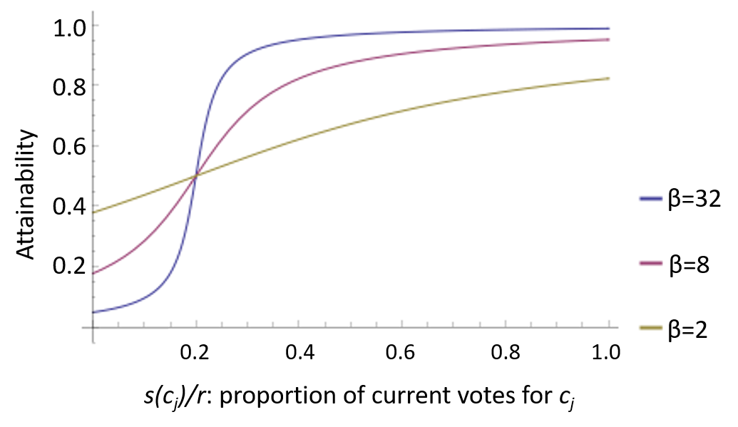
Figure 1: $A_{\beta}(c_{j},s,r)$ for different values of $\beta$ in any single-winner approval election with five candidates.

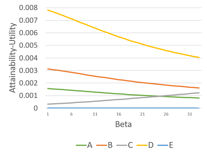
Figure 2: AU score of the five candidates from Scenario B for different values of $\beta$ when $\alpha=1$.

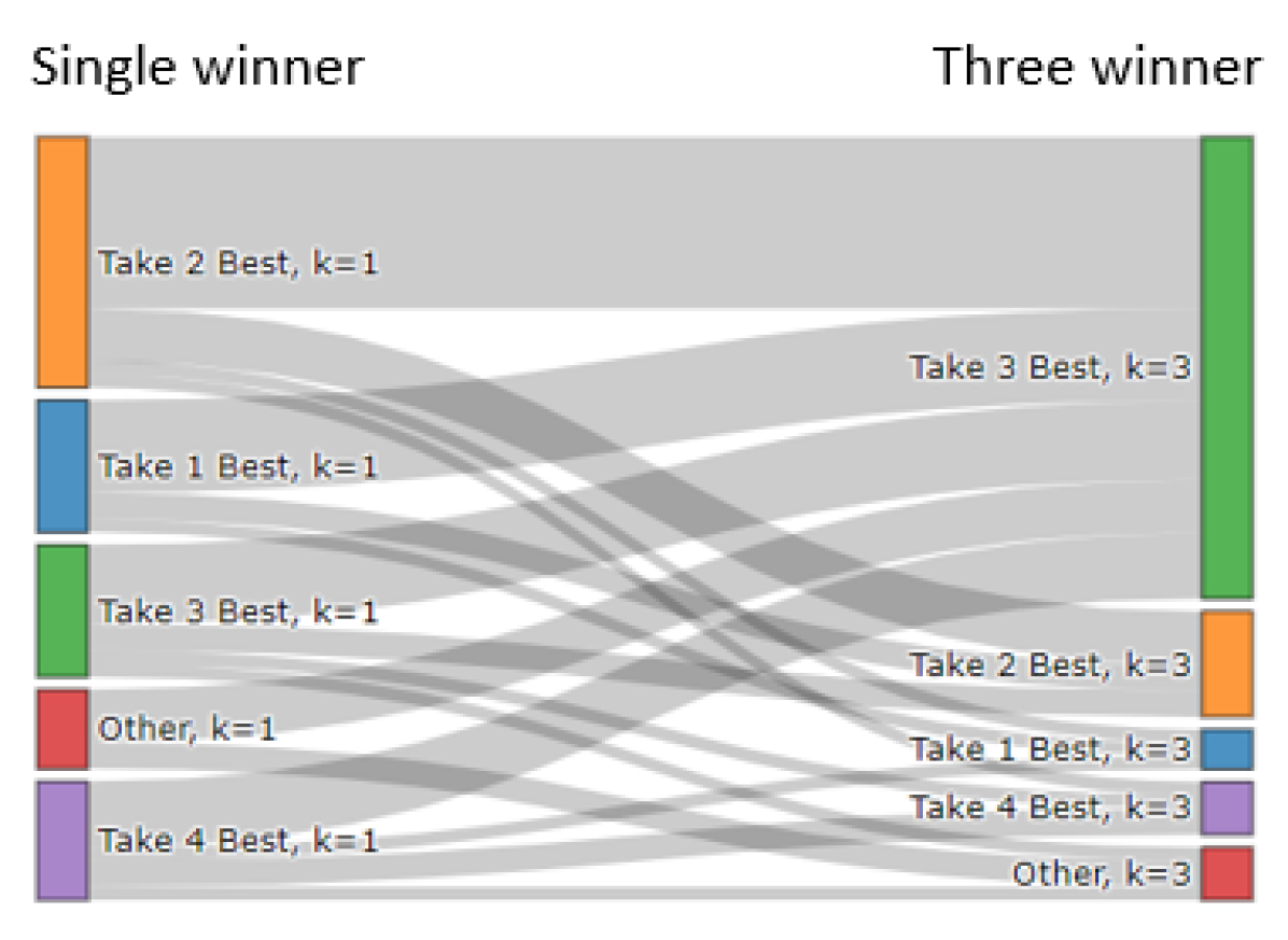
Figure 3: Visualization of the ballots cast by 54 subjects who voted in the single-winner and 3-winner elections with 0 missing votes.

In the plurality setting, the number of current ballots $r$ coincides with the current total number of approvals. This is, of course, not the case in approval voting, where people are allowed to approve up to $m$ candidates. Thus, in our setting, $r$ represents the total number of approvals contained in all ballots that have been currently counted. For example, if we consider an example with five candidates, $m=5$, $A,B,C,D$, and $E$, and $n=5$ voters where two voters have submitted their ballots consisting of $\{A\}$ and $\{A,B,C\}$, we would have $r=4$. We calculate the attainability in an approval election with missing ballots to be the mean attainability over all possible ways in which the remaining ballots can be cast. We model this by considering the set of all possible total approval counts in the election: $T=\{t~{}|~{}r\leq t\leq r+\hat{n}m$}, where $r$ is the number of approvals made so far, $\hat{n}$ is the number of missing ballots and and $\hat{n}m$ represents the number of total possible approvals. In the running example, $\hat{n}=3$, $\hat{n}m=15$, and $T=\{4,5,6,7,\ldots,19\}.$ We can now define the attainability of candidate $c_{j}$ in a multi-winner approval voting setting as:

The utility of a subset of candidates $u(b),b\in\mathcal{P}(C)$ is the sum of the utilities of each candidate $c_{j}$ in $b$. Formally, with a slight abuse of notation, $u(b)=\sum_{c_{j}\in b}u(c_{j})$. Slightly abusing notation, we define the attainability of a set of candidates $b$, as the product of $A_{\beta}(c_{j},s,T)$ for all $c_{j}\in b$ and $1-A_{\beta}(c_{j},s,T)$ for all $c_{j}\notin b$, that is:

We then find a candidate subset $b$ that maximize the trade-off between attainability and utility by incorporating an additional parameter $\alpha\in[0,2]$:

Note that, when $\alpha$ is 0 then the voter only considers attainability, but when $\alpha$ is 2 she only considers utility. A small constant value, $\epsilon$, is also added to account for situations where the left hand component of the equation would result in $0^{0}$, i.e. when candidates have 0 utility and $\alpha=0$.

In Fairstein et al. (2019), voting behavior was predicted for a plurality election, where voters may approve of only one candidate at a time. In multi-winner AV, voters approve as many candidates as they wish, and the top $k$ candidates win the election. When the AU model is applied in the approval setting, voters cast the ballot described by $M^{AU}_{\alpha,\beta}$ as defined in Equation 4. Table 2 shows which ballot is selected by $M^{AU}_{\alpha,\beta}$ for various settings of $\alpha\in\{0,1,2\}$ and $\beta\in\{1,2,\dots,32\}$ on the single winner approval voting election scenario ($s,u,T$) when $s$ and $u$ are described as in Table 3 and $T=\{r\}$ (that is, there are no additional missing ballots). These $\beta$ values were chosen to represent the broad range of shapes that the attainability function can represent as shown in Figure 3.

	$\alpha$
$M^{AU}_{\alpha,\beta}$ ballot	0	1	2
D	$[1..32]$
A,B,C,D,E		$[1]$
A,B,D,E		$[2..8]$
D,E		$[9..21]$
B,D,E		$[22..32]$
A,B,C,E			$[1..32]$

Table 2: Ballots predicted for Scenario A using the attainability-utility model (first column) and corresponding $\beta$ ranges (all other columns) for $\alpha\in\{0,1,2\}$.

Observing Table 2 we note how, in the AU model, $\alpha=0$ predicts a ballot containing only the leading candidate, while $\alpha=2$ predicts the complete ballot of all candidates with positive utility. When $\alpha=1$, different ballots are chosen, depending on the value of $\beta$. Behavior that prioritizes higher utility candidates without voting for leading candidates is not predicted by this model.

It is worth noting that the prediction space for Scenario A, shown in Table 2, predicts only a single Take the X Best strategy (A,B,C,E) and does not predict the optimal ballot ($E$ for 1 winner, 0 missing votes as seen in Table 5). This is counter to the observed behavior where most people used different Take the X Best strategies (see Figure 3). Hence, it is clear that when moving into an approval voting setting, the AU heuristic is inadequate as a model of voter behavior.

The Attainability-Utility with Threshold (AUT) Heuristic

The trade-offs between attainability and utility proposed by Fairstein et al. (2019) are common among cognitive models of decision making (Tversky and Kahneman 1974; Gonzalez-Vallejo 2002) and are cognitively plausible for settings involving a single winner. When applied to multi-winner contexts, the formalization of the trade-offs entails calculating a value for every possible missing ballot (see Formula 4) which becomes increasingly implausible and cognitively demanding as $m$ increases. Hence, we introduce a new model which instead assumes that participants calculate the AU value for each individual candidate, and then choose those candidates that surpass a threshold. This change makes the required mental computations cognitively plausible and is consistent with the adaptive toolbox theory of human decision making (Payne et al. 1993; Gigerenzer and Selten 2002), that people have multiple decision strategies that they choose to match to the environmental constraints of a decision scenario.

More formally, rather than considering the attainability-utility score (AU score) of each $b\in\mathcal{P}(C)$, we calculate the AU score for each individual candidate $c_{j}$:

We introduce a threshold $\tau$ to set the minimum AU score that a voter that will lead to a voter approving $c_{j}$. The introduction of the threshold to the model was inspired by concepts in cognitive psychology (Busemeyer and Townsend 1993). Decision thresholds are parameters that vary predictably based on factors in the environment (such as uncertainty). We expected that using thresholds in our AUT model would outperform AU because it more closely models the cognitive process used to vote in the current paradigm. In approval voting scenarios, the model predicts that a voter will submit a ballot approving of all candidates with an AU score greater than $\tau$. We will refer to this heuristic as attainability-utility with threshold (AUT), and define the corresponding ballot for threshold $\tau$ as:

Figure 3 shows the AU score of each of the five candidates in Scenario B for different values of $\beta$ when $\alpha=1$. We can see that if $\beta=2$, when $\tau=0.007$, and $T=\{r\}$ the model predicts voting for only $D$, while when $\tau=0.001$, then the model predicts voting for $\{A,B,D\}$. Note that for low values of beta, $\{A,B,D\}$ can be predicted by $\tau=0.001$, while high values of beta will lead to a prediction of $\{A,B,C\}$. This exemplifies the flexibility AUT has in generating different ballots. Of special note, is that in single-winner plurality elections where voters can only vote for one candidate, the AUT model simplifies to the AU model, accounting for human voting behavior in both plurality and approval voting.

5 Behavioral Data

Our behavioral study aimed at investigating approval voting heuristics and included 104 participants recruited through Mechanical Turk. Participants were asked to cast ballots in a voting game where they were presented with a number of multi-winner approval voting scenarios with a monetary value that was paid out when certain candidates won. Participants were paid $1.00 to participate in the study and received a bonus of no more than $8.00, which was determined by the outcome of hypothetical elections. All participants voted in the single winner scenarios (n=104). Participants were then randomly assigned to be part of a 2-winner (n=50) or 3-winner (n=54) election for the remainder of the study. More information about this study can be found in the Technical Appendix.

In this analysis, we consider two scenarios in particular, Scenario A and Scenario B, shown in detail in Tables 3 and 4. In these scenarios, the participant faces a situation where each candidate generates a different amount of utility $u\in{0,0.1,0.05,0.10,0.25}$, paid as a reward if that candidate is in the winning set. In both scenarios, none of the participant’s high utility candidates are leading the election, but all are within 1 approval of being tied for the lead. We observe how people respond, particularly considering if they cast a Complete Ballot or a Sincere Ballot, and how many sincere candidates they choose to approve. The experimental data consists of responses to Scenarios A and B in 9 different conditions: where there are 1, 2 and 3-winners with 0, 1 or 3 missing ballots. Hence we can examine how varying both the number of winners as well as the amount of uncertainty affects voter behavior.

Candidate:	A	B	C	D	E
Utility:	0.05	0.10	0.01	0	0.25
# Votes:	3	3	3	4	3

Table 3: Scenario A design, including candidates, utilities and votes. Heuristic votes: Complete: [A,B,C,E], Take 1 Best: [E], Take 2 Best: [E,B], Take 3 Best: [E,B,A]

Candidate:	A	B	C	D	E
Utility:	0.05	0.10	0.01	0.25	0
# Votes:	3	3	4	3	3

Table 4: Scenario B design, including candidates, utilities and votes. Heuristic votes: Complete: [A,B,C,D], Take 1 Best: [D], Take 2 Best: [D,B], Take 3 Best: [D,B,A]

Using $\chi^{2}$ analysis, we examined the responses from both scenarios across all conditions and found no significant difference in the distribution of responses between each scenario. This means that even though the values of the candidates and the current leader changed, the voters behaved largely the same in both Scenarios A and B. Within each scenario, there was also no significant difference in how people voted as the number of missing ballots increased. However, significant differences ($P<0.005$) were found when comparing the strategies used by voters in those conditions electing one or two winners compared to those electing three winners. In general, when voting in single-winner and 2-winner elections, participants cast a ballot for 2 or 3 candidates (single-winner: 57.9%, 2-winner: 70.7%) more often than other strategies. When participants voted in the 3-winner election, they usually cast a ballot for 3 candidates (61.7%). Figure 3 shows how an individual voter’s ballots changed as the number of winners increased from 1 to 3.

We found that, in general, the majority of people vote sincerely with a Take the X Best strategy: 78.8% in Scenario A and 77.8% in Scenario B. However, the value of X used by the voters changed depending on the individual and the size of the winning set, as seen in Figure 3.

6 Evaluation of Heuristics as Models

Using our experimental data, we evaluated five approaches for predicting voter behavior over single-winner, two-winner, and three-winner conditions. First, we consider the effectiveness of a model that predicts optimal votes, i.e., the one that always maximizes the expected utility. We evaluate four other predictive models, each of which corresponds to the heuristics described in Section 4, namely, Complete, Take X Best with X equal to the size $k$ of the winning set, AU and AUT.

Optimal Baseline

As a baseline, we assume that people vote optimally, approving the ballot that maximizes their expected utility, which varies with the number of winners and missing ballots. Given the number of winners $k\in\{1,2,3\}$ and the number of missing ballots $\hat{n}\in\{0,1,3\}$ the expected utility $E$ of ballot $b\in\mathcal{P}(C)$ is: $E(b,k,\hat{n})=\sum_{c_{j}\in b}p(c_{j},k,\hat{n})u(c_{j})$. Assuming that all potential missing ballots are equally likely, $p(c_{j},k,n)$ refers to the probability that candidate $c_{j}$ is elected, given that there are $k$ possible winners, $\hat{n}$ missing votes and that ties are broken uniformly at random.

For each possible number of winners and the number of missing ballots, the Optimal Baseline, selects the ballot maximizing the expected utility:

The optimal ballots and the corresponding maximum expected values for Scenarios A and B can be found in Table 5. Note that the Optimal Baseline in each of these scenarios and conditions corresponds to a variant of the Sincere Ballot of Take the X best. For example, in both scenarios, the Take the 1 Best heuristic is optimal when there is a single winner and no missing ballots. However, it is optimal to Take the 2 Best with 3 winners and no missing ballots.

	# winners ($k$)
$n$	1	2	3
0	Take 1 A: 0.12 B: 0.13	Take 1 A: 0.22 B: 0.26	Take 2 A: 0.31 B: 0.36
1	Take 1 A: 0.11 B: 0.12	Take 2 A: 0.21 B: 0.22	Take 2 A: 0.30 B: 0.31
3	Take 1 A: 0.11 B: 0.11	Take 2 A: 0.20 B: 0.21	Take 2 A: 0.29 B: 0.29

Table 5: The maximum expected utility for Scenarios A and B, and the heuristic that achieves this optimal outcome. $n$ represents the number of missing ballots.

Fitting Heuristics to Data

In addition to the Optimal baseline, we fit each of the four heuristics to the data and tested their accuracy as predictive models of voter behavior. In addition to testing Complete and Take the $X$ Best, where $X$ is set to be the number of winners $X=k$, we trained AU and AUT on the data collected from Scenarios A and B for each individual. The parameters and ranges we considered are:

Attainability-Utility (AU).

Using a grid search, we fit $\alpha\in\{0,1,2\}$ and $\beta\in\{1,2,\dots,32\}$.

Attainability-Utility with Threshold (AUT).

Since the behavioral results did not show a tendency to vote based on attainability alone, i.e., people rarely voted for only leading candidates with no utility or low utility, we choose to set $\alpha=1$ and fit only $\beta$ and $\tau$. Using a grid search, we tested values for $\beta\in\{1,2,\dots,32\}$ and $\tau\in\{0,0.0005,\dots,0.10\}$.

We train the parameters of AU and AUT as follows. For each individual voter, when we fix $k$, we have 6 conditions to use for training and testing our model. These 6 conditions correspond to the number of possible missing ballots, $\hat{n}\in\{0,1,3\}$, for Scenarios A and B. We use five of these observations to train the parameters of the AU or AUT model and predict the sixth. Using a leave-one-out methodology, we do this for all possible splits of the data. We compute the accuracy over these six splits for each individual. We then average this accuracy over all individual voters for each of the $k\in\{1,2,3\}$ winning set size conditions. Each of the models were evaluated for their accuracy in predicting voter behavior in Scenarios A and B. The Optimal, Complete, and Take k Best models are deterministic, depending on the scenario, the number of winners and the number of missing ballots. The average prediction accuracy and standard deviation over the six responses for each of the winning set size conditions are reported in Table 6 and shown in Figure 4.

Evaluation Results and Discussion

The model evaluation results show that a model of optimal behavior using expected utilities is not a good representation of voter behavior and supports the idea that people do not take the time to perform the calculations necessary to identify optimal solutions. We also found that people tend to not vote a Complete Ballot. The experimental data indicated that voters tend to approve more candidates as the size of the winning set increases. Thus, we conjectured that the Take $k$ Best model, predicting that people would vote for the number of top candidates that was equal to the number of winners ($k$) would perform well. However, this was refuted by our experimental results which showed only a modest improvement in performance in the 3-winner condition.

	1 winner	2 winner	3 winner
Optimal:	24.7% (3.9%)	19.7% (9.1%)	14.2% (5.8%)
AU:	13.8% (2.6%)	16.3% (2.0%)	7.4% (2.0%)
Complete:	15.1% (1.2%)	13.7% (2.7%)	9.0% (2.0%)
Take $k$ best:	22.8% (4.1%)	30.7% (2.2%)	58.3% (4.0%)
AUT:	58.1% (11.6%)	68.0% (1.8%)	67.9% (3.4%)

Table 6: Mean prediction accuracy (standard deviation) for each model across conditions.

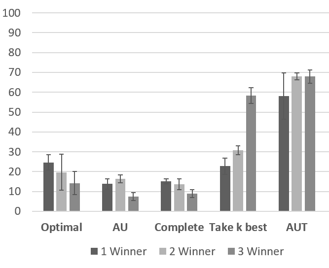
Figure 4: Mean and standard deviation of prediction accuracy for each model across conditions.

Next, we tested whether or not voters make a trade-off between the utility and attainability of the candidates. We first tried this by using the attainability-utility heuristic (AU), which considers the trade-off of attainability and utility for all subsets of candidates. We found that this also does not describe the voting behavior in multi-winner approval voting election. The poor performance of the AU model can likely be attributed to the way that it calculates the attainability-utility for every possible subset of candidates, rather than each individual candidate. The attainability-utility of ballots containing all utility generating candidates is higher than ballots that contain only a subset of them, leading to Complete Ballots being predicted much more often than sincere Take the X Best behavior (See Table 2).

Finally, we addressed this with a novel model of the attainability-utility heuristic with a threshold for approval voting. This model takes into account human cognitive constraints by generating an attainability-utility score for each candidate, rather than for every possible subset, and choosing to vote for only the candidates above a certain threshold. This model performed the best of all the models evaluated. On average, our AUT model performed 80.7% better than the AU model. For single-winner voting, it performed 57.5% better than the second best model (Optimal). In 2-winner elections, it performed 55.0% better than the second best model (Take $k$ Best). Finally, in the 3-winner elections, it performed 14.3% better than the second best model (Take $k$ Best). Hence, our cognitively inspired heuristic model accurately predicts the voting behavior of agents in multi-winner approval voting environments more often than any existing models in the literature.

7 Conclusion and Future Directions

We have evaluated several heuristics as models of voter behavior in multi-winner approval voting. We found that our novel model of the attainability-utility heuristic with threshold provided the best predictive power of the models tested. This model simulates voters ranking each candidate based on a trade-off between attainability and utility, and then approving candidates ranked above a threshold.

To enhance prediction and understanding, a full taxonomy of (internal) cognitive strategies and capabilities along with (external) voting contexts and elements of uncertainty is required to fully explore the interaction between the two. Our AUT model, which describes the trade-off between attainability and utility at the candidate level while generalizing across different conditions of uncertainty, number of winners, and voting rules (i.e. approval and plurality), is an initial step in this direction. Going forward, we will explore how cognitively plausible models like AUT can be used to develop hybrid machine learning models that leverage models of cognitively plausible heuristics to predict voter behavior with even greater accuracy.

Ethics Statement

Our experiments on Mechanical Turk were conducted in an ethical manner and were overseen by the IRB Process at our University, IRB number will be added to the final version (to not break anonymity). All our respondents were paid at least $8.00 per hour of their time.

Our work is meant to advance the understanding of how people vote in realistic settings. Given this, there is always a concern that detailed understanding of how people behave in high stakes decision making environments could be used to adverse ends. However, a better understanding of the heuristics people naturally use may lead us to be able to detect deviations in the future and protect the integrity of election systems.

Acknowledgements

Nicholas Mattei and K. Brent Venable are supported by NSF Award IIS-2007955.

References

- Aziz et al. (2015) Aziz, H.; Gaspers, S.; Gudmundsson, J.; Mackenzie, S.; Mattei, N.; and Walsh, T. 2015. Computational Aspects of Multi-Winner Approval Voting. In Proceedings of the 14th International Joint Conference on Autonomous Agents and Multi-Agent Systems (AAMAS).
- Aziz et al. (2013) Aziz, H.; Gaspers, S.; Mattei, N.; Narodytska, N.; and Walsh, T. 2013. Ties matter: Complexity of manipulation when tie-breaking with a random vote. In Proceedings of the 27th AAAI Conference on Artificial Intelligence (AAAI), 74–80.
- Bowman, Hodge, and Yu (2014) Bowman, C.; Hodge, J. K.; and Yu, A. 2014. The potential of iterative voting to solve the separability problem in referendum elections. Theory and Decision 77(1): 111–124. ISSN 1573-7187. doi:10.1007/s11238-013-9383-2. URL https://doi.org/10.1007/s11238-013-9383-2.
- Brams (1980) Brams, S. J. 1980. Approval voting in multicandidate elections. Policy Studies Journal 9(1): 102.
- Brams (1982) Brams, S. J. 1982. Strategic information and voting behavior. Society 19(6): 4–11.
- Brams and Fishburn (2007) Brams, S. J.; and Fishburn, P. C. 2007. Approval Voting. Springer-Verlag, 2nd edition.
- Brandstätter, Gigerenzer, and Hertwig (2006) Brandstätter, E.; Gigerenzer, G.; and Hertwig, R. 2006. The priority heuristic: making choices without trade-offs. Psychological review 113(2): 409.
- Brandt et al. (2016) Brandt, F.; Conitzer, V.; Endriss, U.; Lang, J.; and Procaccia, A. D., eds. 2016. Handbook of Computational Social Choice. Cambridge University Press.
- Busemeyer and Townsend (1993) Busemeyer, J. R.; and Townsend, J. T. 1993. Decision field theory: a dynamic-cognitive approach to decision making in an uncertain environment. Psychological review 100(3): 432.
- DeMiguel, Garlappi, and Uppal (2007) DeMiguel, V.; Garlappi, L.; and Uppal, R. 2007. Optimal versus naive diversification: How inefficient is the 1/N portfolio strategy? The review of Financial studies 22(5): 1915–1953.
- Endriss (2007) Endriss, U. 2007. Vote manipulation in the presence of multiple sincere ballots. In Proc. 11th Conference on Theoretical Aspects of Rationality and Knowledge (TARK), 125–134.
- Fairstein et al. (2019) Fairstein, R.; Lauz, A.; Meir, R.; and Gal, K. 2019. Modeling People’s Voting Behavior with Poll Information. In Proceedings of the 18th International Joint Conference on Autonomous Agents and Multi-Agent Systems (AAMAS).
- Faliszewski, Hemaspaandra, and Hemaspaandra (2010) Faliszewski, P.; Hemaspaandra, E.; and Hemaspaandra, L. A. 2010. Using Complexity to Protect Elections. Commun. ACM 53(11): 74–82. ISSN 0001-0782. doi:10.1145/1839676.1839696. URL http://doi.acm.org/10.1145/1839676.1839696.
- Faliszewski and Procaccia (2010) Faliszewski, P.; and Procaccia, A. D. 2010. AI’s War on Manipulation: Are We Winning? AI Magazine 31(4): 53–64.
- Gigerenzer and Goldstein (1996) Gigerenzer, G.; and Goldstein, D. G. 1996. Reasoning the fast and frugal way: models of bounded rationality. Psychological Review 103(4): 650.
- Gigerenzer and Selten (2002) Gigerenzer, G.; and Selten, R. 2002. Bounded rationality: The adaptive toolbox. MIT press.
- Gigerenzer and Todd (1999) Gigerenzer, G.; and Todd, P. M. 1999. Fast and frugal heuristics: The adaptive toolbox. In Simple heuristics that make us smart, 3–34. Oxford University Press.
- Gonzalez-Vallejo (2002) Gonzalez-Vallejo, C. 2002. Making trade-offs: A probabilistic and context-sensitive model of choice behavior. Psychological Review 109(1): 137.
- Kilgour (2010) Kilgour, D. M. 2010. Approval Balloting for Multi-winner Elections. In Handbook on Approval Voting, chapter 6. Springer.
- Laslier and Sanver (2010) Laslier, J.-F.; and Sanver, M. R., eds. 2010. Handbook on Approval Voting. Studies in Choice and Welfare. Springer-Verlag.
- Laslier and Van der Straeten (2008) Laslier, J.-F.; and Van der Straeten, K. 2008. A live experiment on approval voting. Experimental Economics 11(1): 97–105.
- Mattei (2020) Mattei, N. 2020. Closing the Loop: Bringing Humans into Empirical Computational Social Choice and Preference Reasoning. In Proceedings of the 29th International Joint Conference on Artificial Intelligence (IJCAI), 5169–5173.
- Mattei, Narodytska, and Walsh. (2014) Mattei, N.; Narodytska, N.; and Walsh., T. 2014. How Hard Is It To Control an Election by Breaking Ties? In Proceedings of the 21st European Conference on Artificial Intelligence (ECAI), 1067–1068.
- Mattei and Walsh (2013) Mattei, N.; and Walsh, T. 2013. PrefLib: A Library for Preferences, http://www.preflib.org. In Proceedings of the 3rd International Conference on Algorithmic Decision Theory (ADT).
- Mattei and Walsh (2017) Mattei, N.; and Walsh, T. 2017. A PrefLib.Org Retrospective: Lessons Learned and New Directions. In Endriss, U., ed., Trends in Computational Social Choice, chapter 15, 289–309. AI Access Foundation.
- Meir (2018) Meir, R. 2018. Strategic Voting. Synthesis Lectures on Artificial Intelligence and Machine Learning. Morgan & Claypool Publishers.
- Meir, Lev, and Rosenschein (2014) Meir, R.; Lev, O.; and Rosenschein, J. 2014. A local-dominance theory of voting equilibria. In Proceedings of the 15th ACM conference on Economics and Computation (ACM EC), 313–330.
- Meir, Procaccia, and Rosenschein (2008) Meir, R.; Procaccia, A. D.; and Rosenschein, J. S. 2008. A broader picture of the complexity of strategic behavior in multi-winner elections. In Proceedings of the 7th International Joint Conference on Autonomous Agents and Multi-Agent Systems (AAMAS), 991–998.
- Meir et al. (2008) Meir, R.; Procaccia, A. D.; Rosenschein, J. S.; and Zohar, A. 2008. Complexity of Strategic Behavior in Multi-Winner Elections. Journal of Artificial Intelligence Research 33: 149–178.
- Mennle et al. (2015) Mennle, T.; Weiss, M.; Philipp, B.; and Seuken, S. 2015. The power of local manipulation strategies in assignment mechanisms. In Proceedings of the 24th International Joint Conference on Artificial Intelligence (IJCAI).
- Niemi (1984) Niemi, R. G. 1984. The Problem of Strategic Behavior under Approval Voting. The American Political Science Review 78(4): 952–958.
- Obraztsova, Elkind, and Hazon (2011) Obraztsova, S.; Elkind, E.; and Hazon, N. 2011. Ties matter: Complexity of voting manipulation revisited. In Proceedings of the 10th International Joint Conference on Autonomous Agents and Multi-Agent Systems (AAMAS), 71–78.
- Payne et al. (1993) Payne, J. W.; Payne, J. W.; Bettman, J. R.; and Johnson, E. J. 1993. The adaptive decision maker. Cambridge university press.
- Regenwetter, Ho, and Tsetlin (2007) Regenwetter, M.; Ho, M.-H. R.; and Tsetlin, I. 2007. Sophisticated approval voting, ignorance priors, and plurality heuristics: A behavioral social choice analysis in a Thurstonian framework. Psychological Review 114(4): 994–1014.
- Reijngoud and Endriss (2012) Reijngoud, A.; and Endriss, U. 2012. Voter response to iterated poll information. In Proceedings of the 11th International Joint Conference on Autonomous Agents and Multi-Agent Systems (AAMAS), 635–644.
- Tal, Meir, and Gal (2015) Tal, M.; Meir, R.; and Gal, Y. 2015. A Study of Human Behavior in Online Voting. In Proceedings of the 14th International Joint Conference on Autonomous Agents and Multi-Agent Systems (AAMAS), 665–673.
- Tversky and Kahneman (1974) Tversky, A.; and Kahneman, D. 1974. Judgment under uncertainty: Heuristics and biases. Science 185(4157): 1124–1131.
- Tyszler and Schram (2016) Tyszler, M.; and Schram, A. 2016. Information and strategic voting. Experimental Economics 19(2): 360–381.
- Walsh (2007) Walsh, T. 2007. Uncertainty in preference elicitation and aggregation. In AAAI, volume 7, 3–8.
- Zou, Meir, and Parkes (2015) Zou, J.; Meir, R.; and Parkes, D. 2015. Strategic Voting Behavior in Doodle Polls. In Proc. of the 18th ACM Conference on Computer Supported Cooperative Work & Social Computing, 464–472.