Adaptive Explicit Kernel Minkowski Weighted K-means

Abstract

The K-means algorithm is among the most commonly used data clustering methods. However, the regular K-means can only be applied in the input space and it is applicable when clusters are linearly separable. The kernel K-means, which extends K-means into the kernel space, is able to capture nonlinear structures and identify arbitrarily shaped clusters. However, kernel methods often operate on the kernel matrix of the data, which scale poorly with the size of the matrix or suffer from the high clustering cost due to the repetitive calculations of kernel values. Another issue is that algorithms access the data only through evaluations of $K(x_{i},x_{j})$, which limits many processes that can be done on data through the clustering task. This paper proposes a method to combine the advantages of the linear and nonlinear approaches by using driven corresponding approximate finite-dimensional feature maps based on spectral analysis. Applying approximate finite-dimensional feature maps were only discussed in the Support Vector Machines (SVM) problems before. We suggest using this method in kernel K-means era as alleviates storing huge kernel matrix in memory, further calculating cluster centers more efficiently and access the data explicitly in feature space. These explicit feature maps enable us to access the data in the feature space explicitly and take advantage of K-means extensions in that space. We demonstrate our Explicit Kernel Minkowski Weighted K-mean (Explicit KMWK-mean) method is able to be more adopted and find best-fitting values in new space by applying additional Minkowski exponent and feature weights parameter. Moreover, it can reduce the impact of concentration on nearest neighbour search by suggesting investigate among other norms instead of Euclidean norm, includes Minkowski norms and fractional norms (as an extension of the Minkowski norms with p<1). The proposed method is evaluated by four benchmark data sets and compared the performance with commonly used kernel clustering approach. Experiments show the proposed method consistently achieves superiors clustering performances while it can be used to reduce memory consumption as well.

Keywords Kernel clustering  $\cdot$ Minkowski metric  $\cdot$ Features map  $\cdot$ K-means

1 Introduction

Clustering can be considered as the most important unsupervised learning problem. Clustering methods are used to determine the intrinsic grouping in a set of unlabeled data. It has been shown to be useful in many practical domains such as web search, image segmentation, image compression, gene expression analysis, recommendation systems and mining text data [4, 17, 8]. K-means clustering [20] is one of the most popular conventional clustering algorithms, despite its age. It aims to partition sample of N observation into K compact clusters in an iterative process. The K-means algorithm only works reasonably well when 1) clusters can be separated by hyper-planes and 2) each data point belongs to the closest cluster center. If one of these principles does not hold, the standard K-means algorithm will likely not give a good result. Kernel-based clustering methods overcome these limitations by using an appropriate non-linear mapping to higher dimensional feature space. Thus, it enables the K-means algorithm to partition data points by the linear separator in the new space, that has non-linear projection back in the original space. Various types of kernel-based methods such as the kernel version of the SOM (Self-organizing map) algorithm [19, 16], kernel neural gas[21], one Class SVM (Support Vector Machines) [2] and kernel fuzzy clustering [26, 25] have been proposed by researchers. In this paper, we focus on kernel k-means clustering because of its efficiency and simpleness. Furthermore, various studies [24, 7, 6] claim that different kernel-based clustering methods show similar result as kernel K-means.

Although kernel-based methods have received considerable attention from the machine learning community in recent years, they still suffer from the following problems in real applications. First, the high clustering cost due to either the repeated calculations of kernel values or requiring huge amounts of memory to store the kernel matrix makes it unsuitable for large corpora. Second, algorithms access the data only through evaluations of K(x, y). Therefore, many processes on the data points like fighting the concentration phenomenon, handling noise, etc. limited to work in the original space.

The aim of this paper is to develop a clustering method that can group data points with both linear and non-linear structures while try to address the two mentioned problems of kernel clustering methods. As the main contribution of this paper, we address both the space complexity of storing kernel matrix and lack of accessing to data in feature space by proposing new Adaptive Explicit Kernel Minkowski Weighted K-means (Explicit KMWK-mean) method. The proposed method combines the advantages of the linear and nonlinear approaches by using driven corresponding approximate finite-dimensional feature maps based on 1D Fourier analysis [23] for a large family of additive kernels, known as $\gamma$-homogeneous kernels. The proposed method, first map data to feature space. This feature space is data independent approximation of $\gamma$-homogeneous kernels. Then, in order to provide a better fit to cluster structure, the weighted version of Minkowski K-means in low-dimensional feature space would be applied. Especially, we analyze the concentration of the Euclidean norm and the impact of distance measure on concentration and investigate on Minkowski norms and fractional norms, an extension of the Minkowski norms with $p<1$, as a measure of distance among data in the kernel space. Adaptive Minkowski metric allows to fight against possible concentration in high-dimensional spaces and the weighting property enables our algorithm to cover spherical and non-spherical (elliptical) structures in feature space and getting the chance of finding even more complex clusters in feature space.

The remainder of this article is organized as follows. Section 2, briefly describes k-means and kernel k-means as the preliminary notions. Section 3 introduces Explicit Feature Maps and especially focused on Homogeneous kernels. Section 4 presents our modified version of kernel K-means by analyzing the alternative Minkowski distance for arbitrary $p\in\mathbb{R}^{+}$ instead of Euclidean one in feature space. In Section 5 we describe the results of experiments four benchmark data sets. Section 6 concludes the paper.

2 K-means and Kernel K-means

The K-means method is designed to partition $N$ D-dimensional samples $X=(x_{1},x_{2},\ldots,x_{N}).$ in to $K$ clusters ${C_{1}}{\rm{,}}{C_{2}}{\rm{,}}...{\rm{,}}{C_{K}}$ and return centroid vector for each cluster $M=(m_{1},m_{2},\ldots,m_{K}).$ The batch mode K-means algorithm would operate by the following iterative procedure:

1. Initialize $K$ cluster center $m_{1},m_{2},\ldots,m_{K}.$

2. Assign each sample $x_{i}$ to its closest center. Namely, compute the indicator matrix ${\delta_{ik}},\>(1\leq k\leq K).$

   $${\delta_{ik}}{\rm{=}}\left\{{\begin{array}[]{*{20}{c}}1&{d({{\rm{x}}_{\rm{i}}},{{\rm{m}}_{\rm{k}}})<d({{\rm{x}}_{\rm{i}}},{{\rm{m}}_{\rm{j}}})\>{\rm{for}}\>{\rm{all}}\>{\rm{j}}\neq k}\\ 0&{otherwise}\end{array}}\right.$$ (1)

3. Update the cluster centers.

   $${m_{k}}=\frac{1}{{|{c_{k}}|}}\sum\limits_{i=1}^{N}{{\delta_{ik}}}{x_{i}}$$ (2)

   where $|C_{k}|$ is the number of samples in $C_{k}$.

4. Iterate between (2) and (3) until convergence.

5. Return $m_{1},m_{2},\ldots,m_{K}.$

Note that, in (1), $d(x_{i},m_{k})$ is the Euclidean distance given by:

$${d^{2}}({x_{i}},{m_{k}})=||{x_{i}}-{m_{k}}|{|^{2}}$$ (3)

The preceding procedure actually is an iterative solution to optimization problem that attempts to minimize the objective function as follows:

$$\arg{\rm{}}\mathop{{\rm{min}}}\limits_{M,\delta}\sum\limits_{i=1}^{N}{\sum\limits_{k=1}^{K}{{\delta_{ik}}||{x_{i}}-{m_{k}}|{|^{2}}}}$$ (4)

In most cases, the distance in use is the squared Euclidean distance. However, the Euclidean distances tend to concentrate, when data are high dimensional. This means that, all the pairwise distances may converge to the same value. Accordingly, the relevance of Euclidean distance has been questioned in the past and alternative norms, especially fractional norms ($L_{p}$ semi-norms with $p<1$) were suggested to reduce concentration phenomenon [13, 1]. Obviously, by using different metrics, cluster centers don’t follow from the equation in (2) anymore. Finding fractional and Minkowski’s centers, whose components are minimizers of the summary corresponding distances, discussed in Section 4.1.3.

The K-means algorithm with Euclidean distance generally works on ellipse-shaped clusters. It is not applicable when elliptical regions does not hold. By applying some kind of transformation to the data, mapping them to some new space, the k-means algorithm may be achieve better performance than in original space. Again, suppose we are given N samples of $X=(x_{1},x_{2},\ldots,x_{N})\>x_{i}\in\mathbb{R}^{D}$, and mapping function $\Phi$ that transforms $x_{i}$ from original space $\mathbb{R}^{D}$ to a high dimensional feature space $\mathbb{H}$. Kernel functions are implicitly defined as the dot product of two vectors in the new transformed feature space.

$$K(x_{i},x_{j})=\Phi(x_{i}).\Phi(x_{j})$$ (5)

In the rest of paper, we use ${\Phi_{i}}$ instead of $\Phi({x_{i}})$ for ease of description. Essentially, the transformation is defined implicitly, without knowing the concrete form of $\Phi$ [22]. Computation of distances in the transformed space is one of the most important issues when K-means is extended to the kernel K-means. The squared Euclidean distance between $x_{i}$ and $x_{j}$ in feature space would be as:

$$\begin{array}[]{l}\begin{array}[]{l}\mathop{{d^{2}}}\limits_{Euc}({\Phi_{i}},{\Phi_{j}})=||{\Phi_{i}}-{\Phi_{j}}|{|^{2}}={\Phi_{i}}^{2}-2{\Phi_{i}}.{\Phi_{j}}+{\Phi_{j}}^{2}\\ =K({x_{i}},{x_{i}})-2K({x_{i}},{x_{j}})+K({x_{j}},{x_{j}})\end{array}\end{array}$$ (6)

The cluster center in transformed space can be calculated as given below:

$${m^{\prime}_{k}}=\frac{1}{{|{C_{k}}|}}\sum\limits_{i=1}^{N}{{\delta_{ik}}}{\Phi_{i}}$$ (7)

Therefore, the distance of each data point and the cluster center in new space can be computed without knowing the transformation $\Phi$ explicitly.

$$\begin{array}[]{*{20}{l}}{d{{}^{2}}({\Phi_{i}},{m^{\prime}_{k}})=||{\Phi_{i}}-\frac{1}{{|{C_{k}}|}}\sum\limits_{j=1}^{N}{{\delta^{\prime}_{jk}}.}{\Phi_{j}}|{|^{2}}}\\ {=K({x_{i}},{x_{i}})-\frac{2}{{|{C_{k}}|}}\sum\nolimits_{{x_{j\in{C_{k}}}}}{K({x_{i}},{x_{j}})}+\frac{1}{{|{C_{k}}{|^{2}}}}\sum\nolimits_{{x_{j\in{C_{k}}}}}{\sum\nolimits_{{x_{l\in{C_{k}}}}}{K({x_{i}},{x_{l}})}}}\end{array}$$ (8)

Where ${\delta^{\prime}}$ is the indicator matrix which ${{\delta^{\prime}_{jk}}}$ indicates whether ${{\Phi_{i}}}$ is assigned to ${{C_{k}}}$ or not. We will be moved from K-means to Kernel K-means by applying(8) to the standard K-means.

The following notation is used in the rest of the paper. Multidimensional additive kernels have been represented as $K(x_{i},x_{j})$, henceforth $k(x_{i},x_{j})$ will be used for the scalar ones. Multidimensional kernel function can be obtained from scalar ones as: $K({x_{i}},{x_{j}})=\sum\limits_{l=1}^{D}k(x_{i}^{l},x_{j}^{l})$. The scalar feature map is also denoted by $\varphi({x_{i}})$ and multidimensional ones are given by ${\Phi_{i}}=\mathop{\oplus}\limits_{l=1}^{D}\varphi_{i}^{l}$, it means ${\Phi_{i}}=[\varphi_{i}^{1},...\varphi_{i}^{D}]$.

3 Explicit Feature Maps

Namely, in kernel learning context, for each positive-definite (PD) kernel $K(x_{i},x_{j})$ there exists a corresponding mapping function $\Phi$ to an arbitrary dimensional space such that $K(x_{i},x_{j})=\Phi_{i}.\Phi_{j}.$ Even though the explicit form of the mapping function is useful conceptually, it is not often used in computations. Typically, these feature spaces are infinite-dimensional, yet it is possible to find an efficient finite-dimensional approximation of $\Phi$. In the following, we will introduce a class of kernels which commonly used in computer vision, called homogeneous kernels. Then describe deriving corresponding approximate explicit finite-dimensional feature maps proposed by Vedaldi and Zisserman [23]. The main focus of this paper, as in an influential paper [23], is a class of additive kernels such as the Hellinger’s, ${\chi^{2}}$, intersection, and Jensen-Shannon ones, which are frequently used in computer vision applications. All of the mentioned kernels are mutual in two properties of additivity and homogeneity. Common homogeneous kernels with their properties are listed in table 1.

Table 1: Well-known kernel functions and their corresponding distance , signature and closed form feature maps. This table is adopted from [23].

Kernel	$K(x,y)$	$d(x,y)$	Signature$\kappa(\lambda)$	$\rho(\omega)$	${\varphi_{\omega}}({x^{i}})$
$\chi^{2}$	$\sum{\frac{{{{({x^{i}}-{y^{i}})}^{2}}}}{{({x^{i}}-{y^{i}})}}}$	$\sum{\frac{{2{x^{i}}{y^{j}}}}{{({x^{i}}+{y^{j}})}}}$	${\rm{sech(}}\lambda/2{\rm{)}}$	${\mathop{\rm sech}\nolimits}(\pi\omega)$	${e^{i\omega{\rm{log}}{{\rm{x}}^{i}}}}\sqrt{{x^{i}}{\rm{sech(}}\pi\omega{\rm{)}}}$
Hellinger	$2\sum{(\sqrt{{x^{i}}}}-\sqrt{{y^{i}}}{)^{2}}$	$\sum{\sqrt{{x^{i}}{y^{i}}}}$	$1$	$\delta(\omega)$	$\sqrt{{x^{i}}}$
JS	$\begin{array}[]{c}\sum{({x^{i}}{{\log}_{2}}(\frac{{2{x^{i}}}}{{{x^{i}}+{y^{j}}}})}+\\ {y^{i}}{\log_{2}}(\frac{{2{y^{i}}}}{{{x^{i}}+{y^{j}}}}))\end{array}$	$\begin{array}[]{c}\frac{1}{2}\sum{({x^{i}}{{\log}_{2}}(\frac{{{x^{i}}+{y^{j}}}}{{{x^{i}}}})}+\\ {y^{j}}{\log_{2}}(\frac{{{x^{i}}+{y^{j}}}}{{{y^{j}}}}))\end{array}$	$\begin{array}[]{c}\frac{{{e^{\frac{\lambda}{2}}}}}{2}{\log_{2}}(1+{e^{-\lambda}})+\\ \frac{{{e^{\frac{{-\lambda}}{2}}}}}{2}{\log_{2}}(1+{e^{\lambda}})\end{array}$	$\frac{2}{{\log 4}}\frac{{{\mathop{\rm sech}\nolimits}(\pi\omega)}}{{1+4{\omega^{2}}}}$	${e^{i\omega{\rm{log}}{{\rm{x}}^{i}}}}\sqrt{\frac{2}{{\log 4}}\frac{{{\mathop{\rm sech}\nolimits}(\pi\omega)}}{{1+4{\omega^{2}}}}}$
intersection	$\sum{|{x^{i}}-{y^{i}}|}$	$\sum{\min({x^{i}},{y^{i}})}$	${e^{\frac{{-|\lambda|}}{2}}}$	$\frac{2}{{\log 4}}\frac{{{\mathop{\rm sech}\nolimits}(\pi\omega)}}{{1+4{\omega^{2}}}}$	${e^{i\omega{\rm{log}}{{\rm{x}}^{i}}}}\sqrt{\frac{2}{\pi}\frac{1}{{1+4{\omega^{2}}}}}$

Homogeneous Kernels.

A kernel $k_{h}(a,b)$ called a homogeneous of degree $\gamma$ if

$$\forall t\geq 0:{K_{h}}(ta,tb)={t^{\gamma}}{K_{h}}(a,b)$$ (9)

Here $a,b\in\mathbb{R}$. If we set $t=\frac{1}{{\sqrt{ab}}}$, the homogeneous kernel can be rewritten as :

$$\begin{array}[]{l}{k_{h}}(a,b)={t^{-\gamma}}{k_{h}}(ta,tb)={(ab)^{\frac{\gamma}{2}}}{k_{h}}(\sqrt{\frac{b}{a}},\sqrt{\frac{a}{b}})\\ ={(ab)^{\frac{\gamma}{2}}}\kappa(\log b-\log a)\end{array}$$ (10)

The scalar function $\kappa$ is called signature function which is used to deriving associated feature map of homogeneous kernel functions. It is defined as :

$$\kappa(\lambda)={k_{h}}({e^{\frac{\lambda}{2}}},{e^{-\frac{\lambda}{2}}}),{\rm{}}\lambda\in{\rm{R,}}$$ (11)

Bochner’s theorem by using Fourier transform of signature function, $\kappa(\lambda)$ can address the problem of which mapping function made the given homogeneous kernel. As a result, the feature map $\varphi$ for $\gamma$-homogeneous kernels will be derived as:

$${\varphi_{\omega}}(a)={e^{-i\omega\log a}}\sqrt{{a^{\gamma}}\rho(\omega)}$$ (12)

where $\omega$ can be viewed as the index of vector dimension and ${\rho(\omega)}$ is the spectrum function and can be obtained from inverse Fourier transform of the signature $\kappa(\lambda)$.

$$\rho(\omega)=\frac{1}{{{{(2\pi)}^{D}}}}\int_{{R^{D}}}{{e^{-i(\omega,\lambda)}}}\kappa(\lambda)d\lambda.$$ (13)

In (12) feature maps are continuous functions but still finite approximation feature maps can be generated by sampling the continuous spectrum and rescaling it. Closed-form of common kernel feature maps are described in table 1. Moreover, Hein and Bousquet [12] introduced a large class of $\gamma$-homogeneous Hilbertian metrics and correspondent kernels which encompasses all previously described kernels in table 1. This class of metrics defined as follows with two parameters $\alpha$ and $\beta$ to be tuned.

$$d_{\alpha|\beta}^{2}(a,b)=\frac{{{2^{\frac{1}{\beta}}}{{({a^{\alpha}}+{b^{\alpha}})}^{\frac{1}{\alpha}}}-{2^{\frac{1}{\alpha}}}{{({a^{\beta}}+{b^{\beta}})}^{\frac{1}{\beta}}}}}{{{2^{\frac{1}{\alpha}}}-{2^{\frac{1}{\beta}}}}}$$ (14)

Function $d$ in Equation (14) is a $\gamma$-homogeneous metric on ${\mathbb{R}^{+}}$ with $\alpha\in[1,\infty]$ and $\beta\in[\frac{1}{2},\alpha]$ or $\beta\in[-\infty,-1]$. The pointwise limit of $d$ when $\alpha\to\beta$ is determined as:

$$\begin{array}[]{l}\lim{\rm{d}}_{\alpha|\beta}^{2}(a,b)=\frac{{{\beta^{2}}{2^{\frac{1}{\beta}}}}}{{\log(2)}}\frac{\partial}{{\partial\beta}}{(\frac{{{a^{\beta}}+{b^{\beta}}}}{2})^{\frac{1}{\beta}}}\\ ={(\frac{{{a^{\beta}}+{b^{\beta}}}}{{\log(2)}})^{\frac{1}{\beta}}}\left[{\frac{{{a^{\beta}}}}{{{a^{\beta}}+{b^{\beta}}}}\log(\frac{{2{a^{\beta}}}}{{{a^{\beta}}+{b^{\beta}}}})+\frac{{{b^{\beta}}}}{{{b^{\beta}}+{b^{\beta}}}}\log(\frac{{2{b^{\beta}}}}{{{a^{\beta}}+{b^{\beta}}}})}\right]\end{array}$$ (15)

Corresponding PD kernel for the above can be taken by:

$$k(a,b)=\frac{1}{2}(-{d^{2}}(a,b)+{d^{2}}(a,0)+{d^{2}}(b,0))$$ (16)

4 Adaptive Explicit Kernel K-means

In this section, we present the Adaptive Explicit Kernel K-means method for homogeneous kernels. Homogeneous kernels have been introduced in the previous section and a data-independent method [23] for deriving approximate finite-dimensional feature maps was described. This class of kernels is a frequently-used measure for histogram image comparison due to its effectiveness rather than linear kernel(Euclidean distance). Using explicit feature maps alleviates issues around the storing huge similarity matrix or repeated calculation of kernel values. Moreover, we use the explicit feature map to take advantage of accessing through the data in feature space. We expect good matching between K-means model and real data structure of data in transformed space by choosing suitable kernel, but we still have this chance to get better fit by extending from the squared Euclidean to arbitrary weighted Minkowski metric in new space. In addition to adding more flexibility, adaptive Minkowski metric allows to fight against possible concentration in high-dimensional spaces. Furthermore, weighting property with reflect to within-cluster feature variances,enables our algorithm to cover spherical and non-spherical (elliptical) structures. In this way, features with smaller within-cluster variances receive a larger weight and features which more evenly distributed across the cluster get a smaller weight.

4.1 Minkowski Metric

The distance we consider here is the Minkowski distance. It can be seen as a generalization of the Euclidean distance, which is defined as below:

$${d_{Mink}}({x_{i}},{x_{j}})=(\sum\limits_{l=1}^{D}{|x_{i}^{l}-x_{j}^{l}{|^{p}}{)^{\frac{1}{p}}}}$$ (17)

Note that, when $0<p<1$ does not hold metrics properties therefore it is not actual metric and the corresponding norm are not are indeed norms. They are not satisfying the triangle inequality. They are usually called prenorms or fractional norms.

4.1.1 Concentration in high-dimensional spaces

Losing discriminative power of Euclidean distance to indexing points in high-dimensional spaces had been shown in the past. This means, as dimension increases, the distance to the nearest point appear to be as the same as the farthest one. This phenomena is known as concentration of distances. This inability of Euclidean distance to distinguish distances in high dimensions caused to alternative distance measures were suggested. In [13] a theoretical analysis of absolute difference between the farthest point distance $d_{max}$ and the closest point distance $d_{min}$ for Minkowski norms is presented. It point out that for D-dimensional i.i.d random vectors $x_{i},(1\leq i\leq N)$

$$C\leq\mathop{\lim}\limits_{d\to\infty}{\rm{E}}(\frac{{{{\max}_{i}}||{x_{i}}|{|_{p}}-{{\min}_{i}}||{x_{i}}|{|_{p}}}}{{{D^{\frac{1}{p}-\frac{1}{2}}}}})\leq(N-1).C$$ (18)

Where C is some constant independent of the distribution of the $x_{i}$. This means the contrast between closest and farthest neighbor on average grows as $D^{\frac{1}{p}-\frac{1}{2}}$. The authors concluded that $l_{1}$ and $l_{2}$ norm may be more relevant than $l_{p}$ when $p\geq 3$. In fact for $l_{p}$ with $(p\geq 3)$, the difference between to the farthest and nearest neighbor goes to $0$ as dimensionality increases. These results encouraged researchers to examine fractional distances, $l_{p}$ distance with $p\in(0,1)$. In [1] authors extended previous work and proposed using fractional distance metric. They has been shown that fractional distance can provide higher relative contrast and meaningful result under same conditions as in (18).
The obtained results in [13] and [1] cannot be used in general when the data are not uniformly distributed. Indeed, it is quite rare that data spread through such spaces.observation of real data shows that high dimensional spaces are mostly empty. In these spaces, it is common that data spread on a sub-manifold. In [10] data distribution instead of data set has been studied. For that purpose the relative variance ratio is proposed which is defined as follows:

$$R{V_{F,p}}=\frac{{\sqrt{Var(||x_{i}|{|_{p}})}}}{{E(||x_{i}|{|_{p}})}}$$ (19)

Similarly to the relative contrast (18), the relative variance can be seen as a measure of concentration. Smaller values of $R{V_{F,p}}$ indicate less concentration. We can see that the shape of distribution $F$ and the value of $p$ might affect the value of the $R{V_{F,p}}$. Therefore, for adjusting the value of $p$, the shape of distribution should be considered too. It is completely possible that the higher relative variance acquired by higher-order norms.

4.1.2 Choosing the Optimal Value of p

In supervised learning tasks like classification, the value of $p$ could be chosen to maximize model accuracy. However, we do not have that access to the class labels in unsupervised learning. In that case, a sensible way of choosing $p$ could be investigating on use of $R{V_{F,p}}$ as an objective to be maximized. Also in [9] the relation between the phenomenon of concentration and hubness has been studied. The authors proposed an unsupervised approach for choosing the value of $p$ by measuring hub and anti-hub occurrence as defined in the paper. Although $R{V_{F,p}}$ and hubness can give a sense of the concentration level, they are not excellent measures all the time. As shown in Figure (1), a different value of $p$ reflects a distinctive measure of distance in a Euclidean space. It can be seen, the rotation of the coordinate system will also lead to changes in the distance measurement. The only exception is the circular shape, $p=2$ (Figure 1(d)). By adopting $p\to 0$ being exact in one dimension has more value than have balance in two (Figure 1(a)). conversely, by approaching $p\to\infty$, just the maximum difference is matter (Figure 1(f)). So by going far from $p=2$, the distance meaning completely changes therefore the value of $p$ should be chosen by considering both being meaningful and reduction of the concentration. However, ground truth annotation is often costly and inaccessible in real-world applications, there are usually limited available class labels. In this case, semi-supervised learning provides a better choice by leveraging unlabeled data by using a small set of labeled data. We discover the optimal value of exponent $p$, by uncovering only a few percents of data. We employ the entire data set, either labeled or not to run a series of clustering experiments at various values of $p$ as reported superior results rather than using only labeled data in [5].

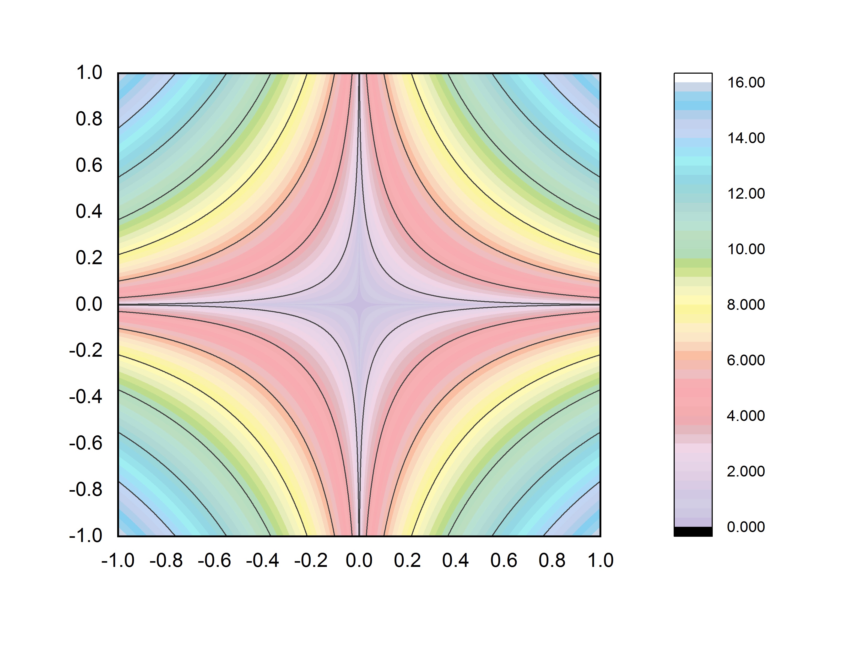
(a) p=0.25

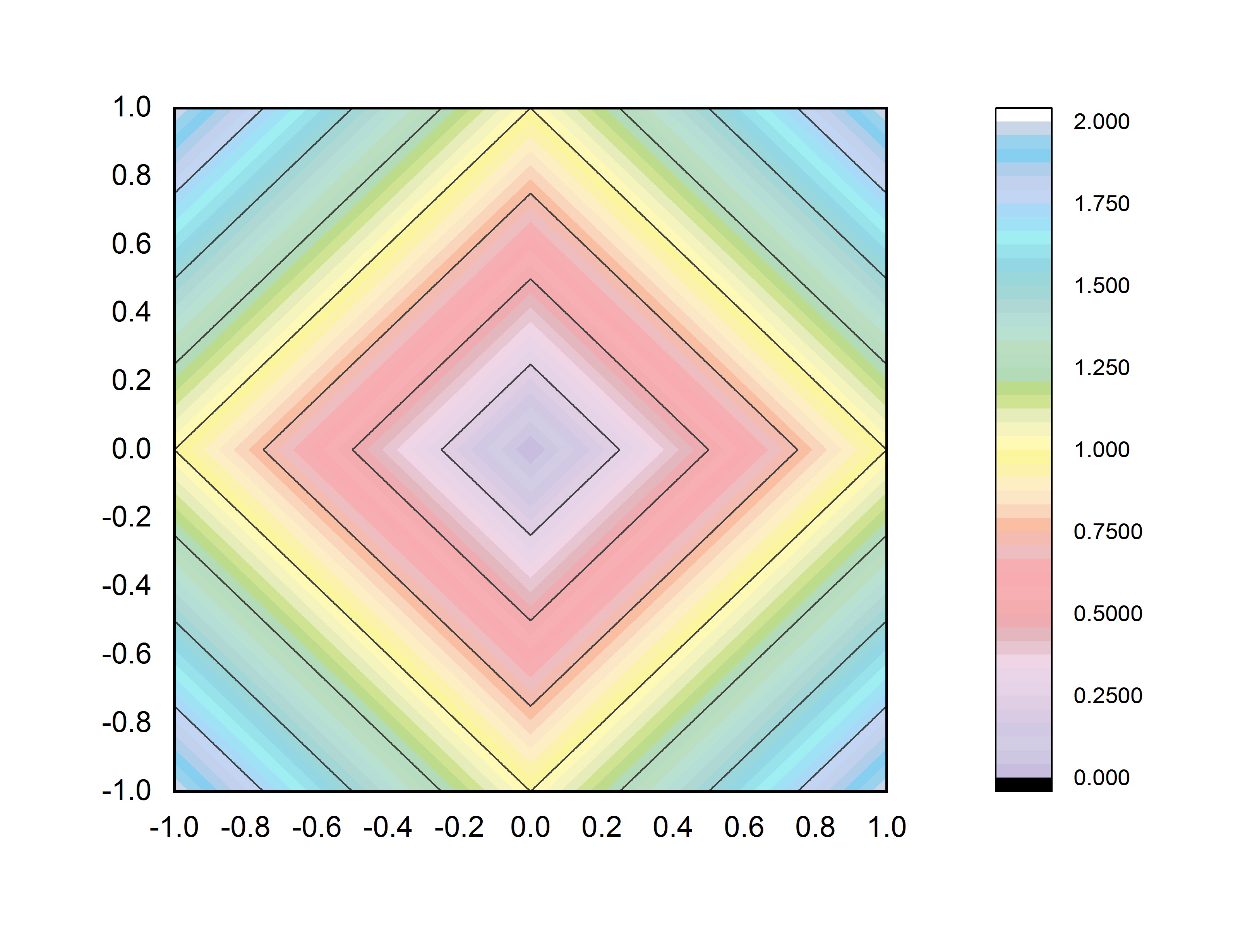
(b) p=1

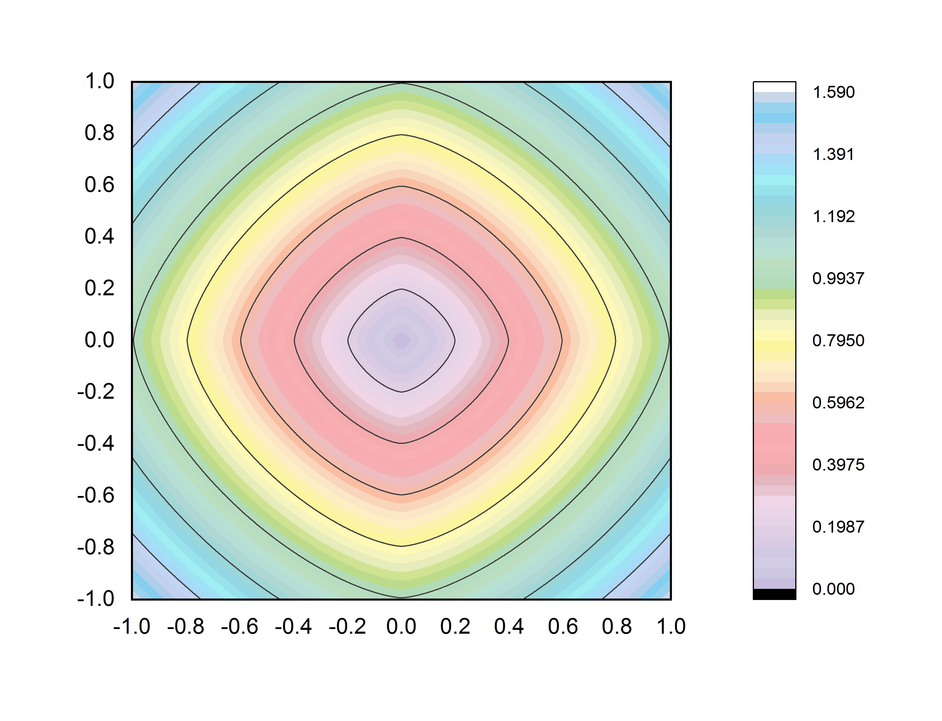
(c) p=1.5

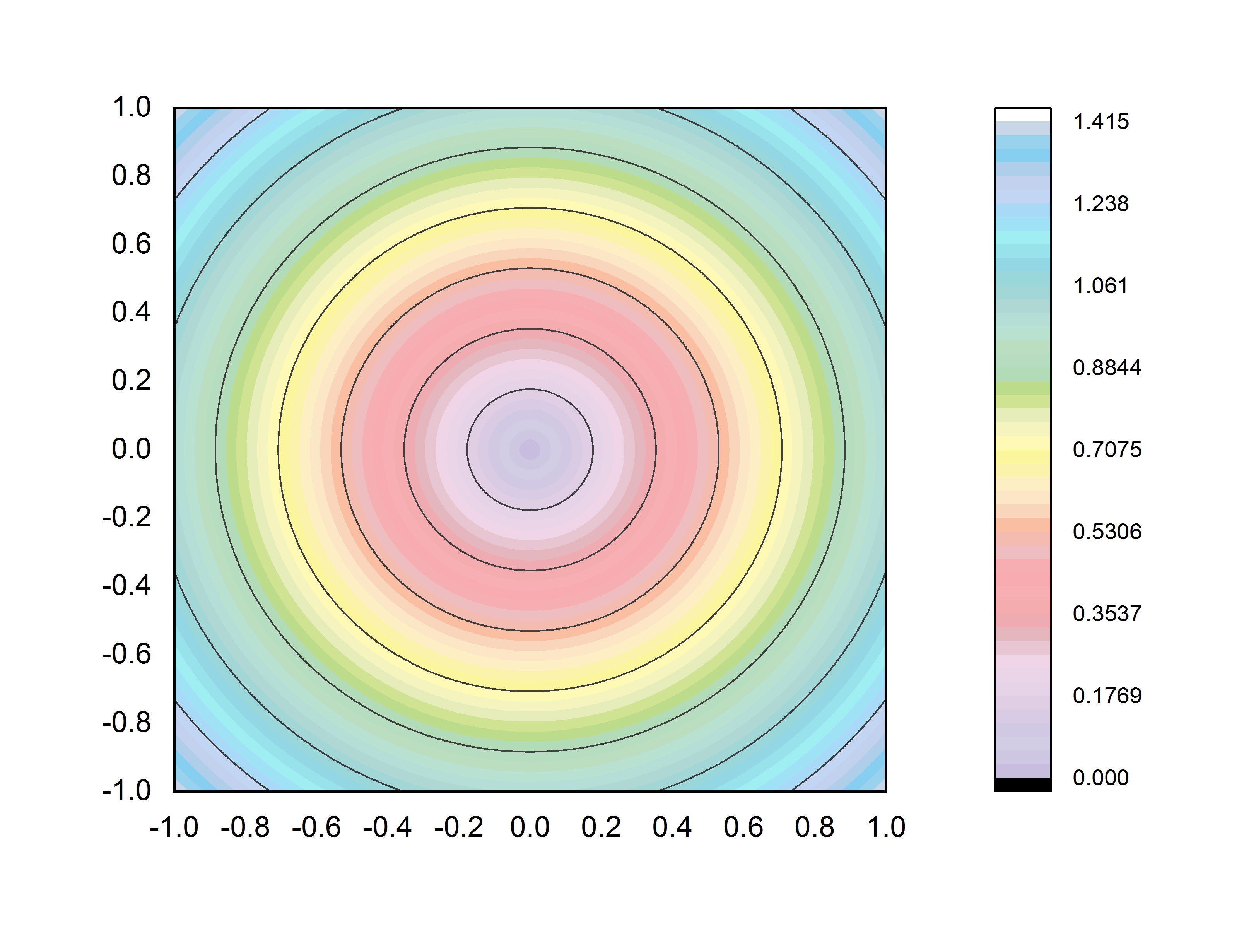
(d) p=2

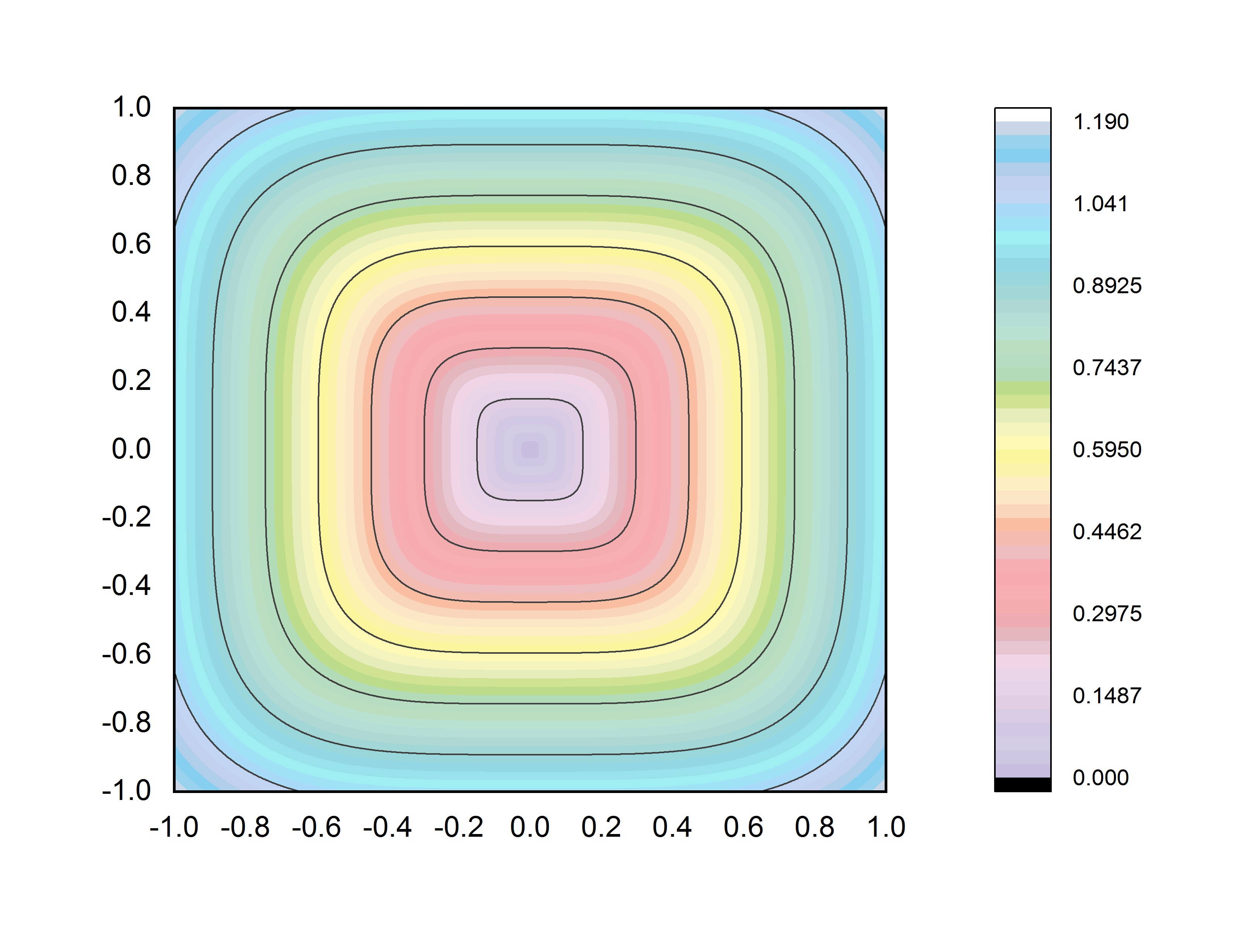
(e) p=4

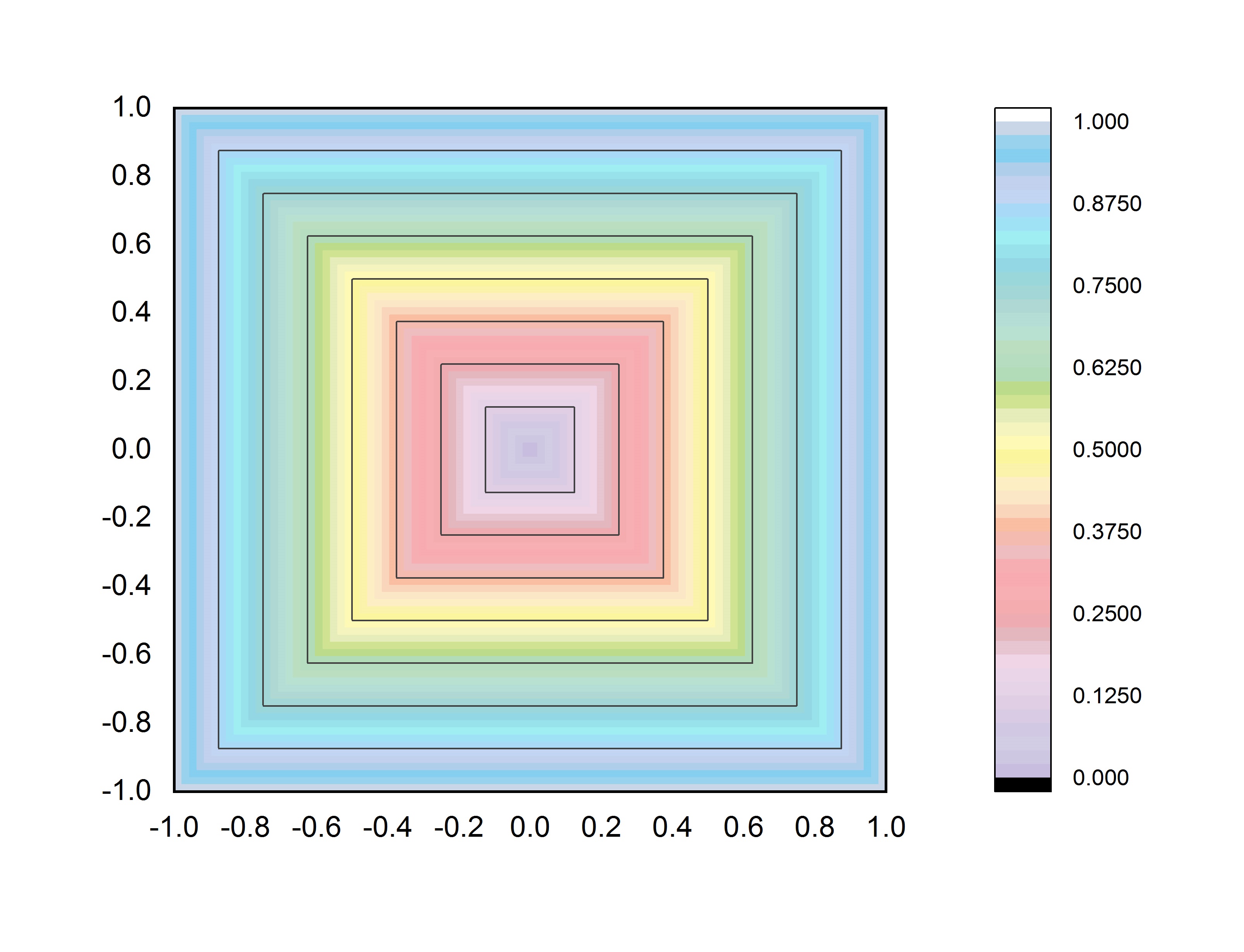
(f) p=$\infty$

Figure 1: Isosimilarity contour lines with eight different values of $p$ in the Minkowski distance formula

4.1.3 Finding Centers

After deriving the approximate feature map and an optimal value for $p$ then the kernel clustering algorithm can be started in order to optimize the objective function with considering Minkowski distance. It minimizes the sum of Minkowski distances between instances and the related centers. The Minkowski k-means objective function can be written as below by applying Minkowski distance on (4).

$$\arg\mathop{{\rm{min}}}\limits_{M^{\prime},\delta}\sum\limits_{i=1}^{N}{\sum\limits_{k=1}^{K}{{\delta_{ik}}||{\Phi_{i}}-{{m}^{\prime}_{k}}|{|^{p}}}}$$ (20)

It should be considered that, it is not possible to use the definition of the center which previously used as Eq (2) since it does not minimize (20) when $\delta$ is given constant. In the other words, For finding Minkowski’s centers, we need to find value of vector $m^{\prime}_{k}$ for each cluster, minimizes the following function:

$$\arg\mathop{{\rm{min}}}\limits_{{{m}^{\prime}_{k}}}{\rm{}}{\sum\limits_{{\Phi_{i}}\in{C_{k}}}{|{\Phi_{i}}-{{m}^{\prime}_{k}}|}^{p}}$$ (21)

Being minimizer of (21) is required for vector $m^{\prime}_{k}$ in order to prove the convergence of Minkowski K-means to a local optimum. In other words, it lowers the cost in each iteration monotonically. By this way, it is proven that the algorithm will be converged in a finite number of iterations since the algorithm iterates a function whose domain is a finite set and the cost is decreased monotonically.
 The search space in order to find vector $m^{\prime}_{k}$ is too large for an exhaustive search because the algorithm needs accurate solutions. Note that finding vector $m^{\prime}_{k}$ is a single objective problem and elements on different dimensions are independent. Various evolutionary algorithms can be designed to find the best solutions. However, for $p>1$ the Eq (21) is a convex function and more desirable algorithms like steepest descent can be used to find the global minimizer [5].

4.2 Weighted Version of Explicit Kernel K-means

Using the feature weighted version of Minkowski distance enables the algorithm to provide a better fit to the cluster structures than is possible with Minkowski K-means alone. It allows our algorithm to find both spherical and non-spherical (elliptical) structural clusters in feature space; accordingly, gives a much better fit to arbitrary shaped clusters in original spaces. Authors in [5] have extended weighted K-means variants work [3, 14, 15] through transforming feature weights to be feature scale. This means Minkowski exponent is assigned to feature weights too. The objective function for the weighted version of Minkowski K-means in Equation (20) can be written as the following equation:

$$\arg\mathop{{\rm{min}}}\limits_{M^{\prime},\delta,W}\sum\limits_{i=1}^{N}{\sum\limits_{k=1}^{K}{\sum\limits_{l=1}^{D^{\prime}}{{\delta_{ik}}{{({w_{kl}})}^{p}}||\Phi_{i}^{l}-m_{k}^{{}^{\prime}l}|{|^{p}}}}}$$ (22)

The weight $w_{kl}$ reflects the relevance of feature $l$ at the cluster $k$. They are assigned base on inverse proportion of dispersion of a feature within a certain cluster. Thus, a feature with small dispersion within a specific cluster would have a higher weight, and vice versa. More precisely, $w_{kl}$ is updated on each iteration as Equation (23), where ${V_{kl}}=\sum\nolimits_{i\in{c_{k}}}{|\varphi({x_{iv}})-{m_{kv}}{|^{p}}}$

$${w_{kv}}=\frac{1}{{\sum\nolimits_{u\in V}{{{(\frac{{{V_{kl}}}}{{{V_{ku}}}})}^{\frac{1}{{p-1}}}}}}}$$ (23)

To see the entire algorithm process easily we have also the following flowchart (Fig. 2):

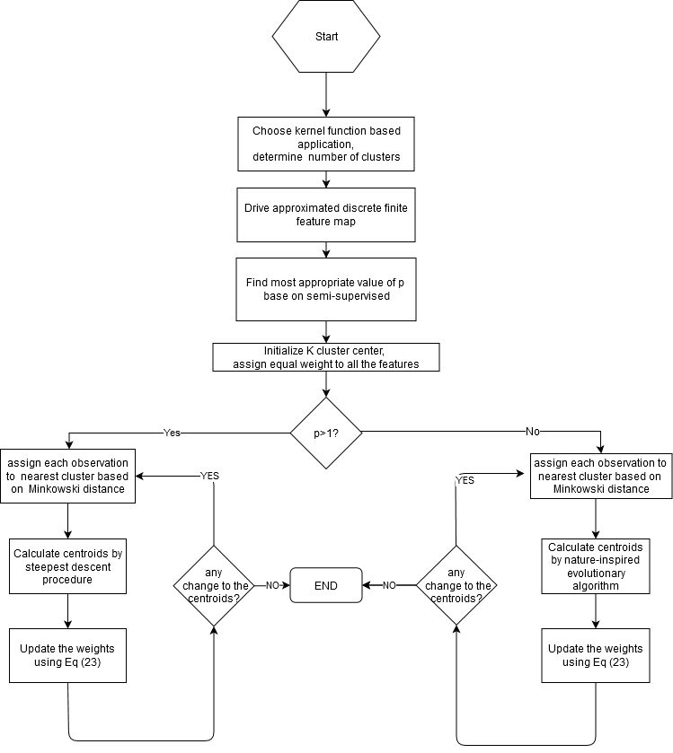
Figure 2: The process flowchart of the Explicit kernel MWK-means algorithm

4.3 Accelerate Minkowski K-means clustering

The Minkowski’s center computation would significantly decelerate the running time. We know already, that at $p=2$ the center is the mean, and at $p=1$ it is given by the component-wise median. Otherwise, it requires an iterative, steepest descent process or an evolutionary computation that can be considered in computation costs. A significant computational speed-up can be achieved by appropriate initialization in order to lessen the number of iterations and consequently decrease the time of searching for Minkowski centers as a process of minimization. We use an output vector containing cluster centers of K-means with $p$ equal 2 or 1 as an initialization. This initialization approach results in an impressive reduction in the time required for clustering, because all of these Minkowski’s distances share the same properties and data would be half-clustered. In [11], the effect of the initialization of K-Means has been studied. The authors found when the clusters overlap, considering various strategies for initialization would not matter much on the results.

5 Experimental Results

In this section, We present the results of performance experiments of our Explicit Kernel MWK-means. We have conducted our experiments on four benchmark data sets: USPS dataset, MNIST dataset, caltech101, and MSRC-V1. Some relevant statistics of them are shown in Table 2.

Table 2: Description of the data sets

	# instances	# features	# classes
MNIST Digits	70,000	784	10
USPS Digits	11,000	256	10
Caltech7	441	60,000	7
MSRC-V1	210	68160	7

Two standard metrics were used to measure the performance of the image clustering that is, Normalized Mutual Information (NMI) and Purity.

5.1 Data Descriptions

MNIST Dataset introduced by Yann Lecun and Corinna Cortes. The dataset includes a total of 70,000 samples of digits 0-9. Each sample consists of 28 by 28 pixels which are within the range [ 0,255 ].

USPS dataset includes 11,000 0-9 digits instances. The dataset is known to be very complicated with a recorded human error rate of 2.5% . The images are 16 by 16 gray-scale pixels.

Caltech101 dataset comprises 9144 images of items belonging to 101 classes and one background class. The number of images in each class differs. The size of each image is approximately 300$\times$200 pixels. We have selected the commonly used 7 groups, i.e. Face, Motorbike, Dolla-Bill, Garfield, Snoopy, Stop-sign and Windsor-chair for our experiments.

MSRC-V1 dataset is from Microsoft Research in Cambridge. This data set is commonly used for scene recognition. We adopt Lee and Grauman’s approach [18] to refine and getting 7 classes including tree, building, airplane, cow, face, car and bicycle where each class has 30 images.

5.2 Setting of the Experiments

To figure out which value of the exponent $p$ has the best performance, a semi-supervised manner was employed. The value of $p$ was derived from uncovering the class of labels on a 15% data sample though clustering was conducted over the whole dataset. After running a series of clustering experiments at different values of $p$, the $p$ that produced the higher clustering accuracy was picked. Each of the experiments repeated 50 times and the average NMI is reported.

Images clustering by using raw pixels as features is unlikely to work effectively. The standard practice is to use visual descriptors such as HOG and SIFT. Both of HOG and SIFT use histograms of pixel intensity gradients in their descriptors. The class of homogeneous kernels are popular due to its effectiveness. Hog can describe the shape and edge information of object; and SIFT features are invariant to image scale, rotation, noise and illumination changes. For MNIST and USPS databases the HOG feature is used. We choose $4\times 4$ grid cells, $2\times 2$ cells in one block and 1 cell spacing as the parameter in HOG calculation. For the two other datasets, Caltech7 and MSRC-V1, the key-points are extracted from each image then represented each keypoint as a 128-dimensional SIFT descriptor. A randomly chosen subset of SIFT features were clustered in order to form a visual vocabulary for either of dataset. Each SIFT descriptor was then quantified into a visual word by considering the nearest cluster center. A 500-dimensional vector representation for each image is obtained.

5.3 Comparison Results

Table 3 clearly shows the match between the value of $p$ learned in semi-supervised and fully supervised settings. The only exception is on MNIST with Using ${\chi^{2}}$ kernel that there is no match between learned and optimal value of exponent $p$. However, table 4 shows it has still better performance than common kernel K-means with the exponent $p=2$.

Table 3: The effect of $p$ on clustering accuracy results with the semi-supervised learning by revealing the class of labels on a 15% of data

	Exponent p		NMI
	learned	Optimal	learned	Optimal
MNIST (intersection)	1.83	1.87	0.7862	0.7981
MNIST (JS)	1.7	1.7	0.7692	0.7692
MNIST(${\chi^{2}}$)	1.7	3.1	0.7772	0.7862
USPS (intersection)	1.66	1.5	0.7212	0.7420
USPS (JS)	1.4	1.4	0.7353	0.7353
USPS (${\chi^{2}}$)	1.4	1.2	0.7291	0.7510
Caltech7 (intersection)	1.1	1	0.6558	0.6661
Caltech7 (JS)	1.1	0.9	0.6203	0.6367
Caltech7 (${\chi^{2}}$)	0.9	1.2	0.6547	0.6706
MSRC-V1 (intersection)	1.22	1	0.7228	0.7438
MSRC-V1 (JS)	1.2	1.1	0.7358	0.7559
MSRC-V1 (${\chi^{2}}$)_	1.3	1.1	0.7565	0.7646

We compared the clustering performance of our method (Explicit kernel MWK-means) with their respective equal weighted version and constant Euclidean one. In addition, we also compared the results of our method with the exact kernel K-means clustering. Table tables 4, 5, 6 and 7 demonstrate the clustering results in terms of NMI and purity on all data sets. It can be seen that, compared with common exact kernel K-means counterparts, our proposed Explicit kernel MWK-means improve the clustering performance on all the data sets.

Table 4: MNIST Digits: Adaptive Explicit kernel MWK-means after using HOG descriptor

		intersection		${\chi^{2}}$		JS
	dm.	NMI	Purity	NMI	Purity	NMI	Purity
Exact Kernel	–	0.7101$\pm$0.024	0.7388$\pm$0.040	0.7109$\pm$0.029	0.7047$\pm$0.044	0.7121$\pm$0.031	0.7007$\pm$0.041
Explicit Kernel K-means	3	0.7138$\pm$0.023	0.7388$\pm$0.040	0.7186$\pm$0.028	0.7107$\pm$0.045	0.7148$\pm$0.033	0.7027$\pm$0.042
Explicit kernel MK-means	3	0.7362$\pm$020	0.7380$\pm$0.038	0.7192$\pm$0.029	0.6868$\pm$0.043	0.7272$\pm$0.035	0.7127$\pm$0.045
Explicit kernel MWK-means	3	0.7862$\pm$0.026	0.8048$\pm$0.039	0.7772$\pm$0.031	0.7909$\pm$0.047	0.7692$\pm$0.038	0.7935$\pm$0.045

Table 5: USPS Digits: Adaptive Explicit kernel MWK-means after using HOG descriptor

		intersection		${\chi^{2}}$		JS
	dm.	NMI	Purity	NMI	Purity	NMI	Purity
Exact Kernel	–	0.6567$\pm$0.040	0.6981$\pm$0.052	0.6695$\pm$0.046	0.6932$\pm$0.057	0.6506$\pm$0.034	0.6976$\pm$0.045
Explicit Kernel K-means	3	0.6591$\pm$0.048	0.6986$\pm$0.056	0.6631$\pm$0.045	0.7006$\pm$0.057	0.6621$\pm$0.036	0.6923$\pm$0.044
Explicit kernel MK-means	3	0.68962$\pm$044	0.7087$\pm$0.055	0.6953$\pm$0.049	0.7107$\pm$0.059	0.6991$\pm$0.037	0.7029$\pm$0.045
Explicit kernel MWK-means	3	0.7212$\pm$0.045	0.7578$\pm$0.055	0.7291$\pm$0.043	0.7658$\pm$0.050	0.7353$\pm$0.039	0.7643$\pm$0.047

Table 6: Caltech7: Adaptive Explicit kernel MWK-means after using SIFT descriptor

		intersection		${\chi^{2}}$		JS
	dm.	NMI	Purity	NMI	Purity	NMI	Purity
Exact Kernel	–	0.6064$\pm$0.018	0.6581$\pm$0.028	0.5918$\pm$0.014	0.6849$\pm$0.023	0.5649$\pm$0.019	0.6710$\pm$0.025
Explicit Kernel K-means	3	0.5961$\pm$0.019	0.6941$\pm$0.027	0.5981$\pm$0.014	0.6858$\pm$0.021	0.5919$\pm$0.017	0.6735$\pm$0.023
Explicit kernel MK-means	3	0.6158$\pm$0.021	0.6987$\pm$0.025	0.6147$\pm$0.025	0.6926$\pm$0.028	0.5803$\pm$0.018	0.6635$\pm$0.022
Explicit kernel MWK-means	3	0.6558$\pm$0.024	0.7581$\pm$0.028	0.6547$\pm$0.026	0.7419$\pm$0.029	0.6203$\pm$0.021	0.7159$\pm$0.025

Table 7: MSRC-v1: Adaptive Explicit kernel MWK-means after using SIFT descriptor

		intersection		${\chi^{2}}$		JS
	dm.	NMI	Purity	NMI	Purity	NMI	Purity
Exact Kernel	–	0.6509$\pm$0.024	0.7201$\pm$0.029	0.6889$\pm$0.028	0.7301$\pm$0.031	0.6859$\pm$0.034	0.7407$\pm$0.039
Explicit Kernel K-means	3	0.6504$\pm$0.022	0.7221$\pm$0.023	0.6927$\pm$0.030	0.7343$\pm$0.034	0.6893$\pm$0.035	0.7436$\pm$0.040
Explicit kernel MK-means	3	0.6728$\pm$0.027	0.7256$\pm$0.032	0.7058$\pm$0.032	0.7390$\pm$0.034	0.7065$\pm$0.033	0.7541$\pm$0.037
Explicit kernel MWK-means	3	0.7228$\pm$0.026	0.8105$\pm$0.030	0.7556$\pm$0.033	0.8269$\pm$0.036	0.7358$\pm$0.030	0.8254$\pm$0.034

6 Conclusions

In this paper, we proposed a kernel K-means method which is based on explicit feature maps with further matching in feature space. Using adaptive Minkowski metric and feature weighting in feature space enable our algorithm to get high clustering quality and show strong robustness to noise feature and concentration phenomena. Applying approximate finite-dimensional feature maps were only discussed in the Support Vector Machines (SVM) problems before. We suggested using this method as alleviates storing huge kernel matrix in memory, in addition to access the data explicitly in feature space. Our experiments demonstrate that our proposed method consistently achieves superiors clustering performances in terms of two standard metrics Normalized Mutual Information (NMI), and Purity, evaluated on four standard bench-mark data sets on object and scene recognition.

References

- [1] Charu C Aggarwal, Alexander Hinneburg and Daniel A Keim “On the surprising behavior of distance metrics in high dimensional space” In International conference on database theory, 2001, pp. 420–434 Springer
- [2] Francesco Camastra and Alessandro Verri “A novel kernel method for clustering” In IEEE transactions on pattern analysis and machine intelligence 27.5 IEEE, 2005, pp. 801–805
- [3] Elaine Y Chan, Wai Ki Ching, Michael K Ng and Joshua Z Huang “An optimization algorithm for clustering using weighted dissimilarity measures” In Pattern recognition 37.5 Elsevier, 2004, pp. 943–952
- [4] Srivatsava Daruru, Nena M Marin, Matt Walker and Joydeep Ghosh “Pervasive parallelism in data mining: dataflow solution to co-clustering large and sparse netflix data” In Proceedings of the 15th ACM SIGKDD international conference on Knowledge discovery and data mining, 2009, pp. 1115–1124 ACM
- [5] Renato Cordeiro De Amorim and Boris Mirkin “Choosing lp norms in high-dimensional spaces based on hub analysis” In Pattern Recognition 45 Elsevier, 2012, pp. 1061–1075
- [6] Inderjit S Dhillon, Yuqiang Guan and Brian Kulis “A unified view of kernel k-means, spectral clustering and graph cuts” Citeseer, 2004
- [7] Chris Ding, Xiaofeng He and Horst D Simon “On the equivalence of nonnegative matrix factorization and spectral clustering” In Proceedings of the 2005 SIAM international conference on data mining, 2005, pp. 606–610 SIAM
- [8] Richard Dubes and Anil K. Jain “Clustering methodologies in exploratory data analysis” In Advances in computers 19 Elsevier, 1980, pp. 113–228
- [9] Arthur Flexer and Dominik Schnitzer “Choosing lp norms in high-dimensional spaces based on hub analysis” In Neurocomputing 169 Elsevier, 2015, pp. 281–287
- [10] Damien Francois, Vincent Wertz and Michel Verleysen “The concentration of fractional distances” In IEEE Transactions on Knowledge and Data Engineering 19.7 IEEE, 2007, pp. 873–886
- [11] Pasi Fränti and Sami Sieranoja “How much can k-means be improved by using better initialization and repeats?” In Pattern Recognition 93 Elsevier, 2019, pp. 95–112
- [12] Matthias Hein and Olivier Bousquet “Hilbertian metrics and positive definite kernels on probability measures” Max Planck Institute for Biological Cybernetics, 2004
- [13] Alexander Hinneburg, Charu C Aggarwal and Daniel A Keim “What is the nearest neighbor in high dimensional spaces?” In 26th Internat. Conference on Very Large Databases, 2000, pp. 506–515
- [14] Joshua Zhexue Huang, Michael K Ng, Hongqiang Rong and Zichen Li “Automated variable weighting in k-means type clustering” In IEEE transactions on pattern analysis and machine intelligence 27.5 IEEE, 2005, pp. 657–668
- [15] Joshua Zhexue Huang, Jun Xu, Michael Ng and Yunming Ye “Weighting method for feature selection in k-means” In Computational Methods of feature selection Chapman & Hall, CRC, 2008, pp. 193–209
- [16] Ryo Inokuchi and Sadaaki Miyamoto “LVQ clustering and SOM using a kernel function” In 2004 IEEE International Conference on Fuzzy Systems (IEEE Cat. No. 04CH37542) 3, 2004, pp. 1497–1500 IEEE
- [17] Daxin Jiang, Chun Tang and Aidong Zhang “Cluster analysis for gene expression data: a survey” In IEEE Transactions on Knowledge & Data Engineering IEEE, 2004, pp. 1370–1386
- [18] Yong Jae Lee and Kristen Grauman “Foreground focus: Unsupervised learning from partially matching images” In International Journal of Computer Vision 85.2 Springer, 2009, pp. 143–166
- [19] Donald MacDonald and Colin Fyfe “The kernel self-organising map” In KES’2000. Fourth International Conference on Knowledge-Based Intelligent Engineering Systems and Allied Technologies. Proceedings (Cat. No. 00TH8516) 1, 2000, pp. 317–320 IEEE
- [20] James MacQueen “Some methods for classification and analysis of multivariate observations” In Proceedings of the fifth Berkeley symposium on mathematical statistics and probability 1.14, 1967, pp. 281–297 Oakland, CA, USA
- [21] A Kai Qin and Ponnuthurai N Suganthan “Kernel neural gas algorithms with application to cluster analysis” In Proceedings of the 17th International Conference on Pattern Recognition, 2004. ICPR 2004. 4, 2004, pp. 617–620 IEEE
- [22] John Shawe-Taylor and Nello Cristianini “Support vector machines” In An Introduction to Support Vector Machines and Other Kernel-based Learning Methods Cambridge University Press, 2000, pp. 93–112
- [23] Andrea Vedaldi and Andrew Zisserman “Efficient additive kernels via explicit feature maps” In IEEE transactions on pattern analysis and machine intelligence 34.3 IEEE, 2012, pp. 480–492
- [24] Hongyuan Zha et al. “Spectral relaxation for k-means clustering” In Advances in neural information processing systems, 2002, pp. 1057–1064
- [25] Dao Q Zhang and Song C Chen “Kernel-based fuzzy and possibilistic c-means clustering” In Proceedings of the International Conference Artificial Neural Network 122, 2003, pp. 122–125
- [26] Dao-Qiang Zhang and Song-Can Chen “A novel kernelized fuzzy c-means algorithm with application in medical image segmentation” In Artificial intelligence in medicine 32.1 Elsevier, 2004, pp. 37–50