Quantum Quasi-Monte Carlo algorithm for out-of-equilibrium Green functions at long times

Abstract

We extend the recently developed Quantum Quasi-Monte Carlo (QQMC) approach to obtain the full frequency dependence of Green functions in a single calculation. QQMC is a general approach for calculating high-order perturbative expansions in power of the electron-electron interaction strength. In contrast to conventional Markov chain Monte Carlo sampling, QQMC uses low-discrepancy sequences for a more uniform sampling of the multi-dimensional integrals involved and can potentially outperform Monte Carlo by several orders of magnitudes. A core concept of QQMC is the a priori construction of a “model function” that approximates the integrand and is used to optimize the sampling distribution. In this paper, we show that the model function concept extends to a kernel approach for the computation of Green functions. We illustrate the approach on the Anderson impurity model and show that the scaling of the error with the number of integrand evaluations $N$ is $\sim 1/N^{0.86}$ in the best cases, and comparable to Monte Carlo scaling $\sim 1/N^{0.5}$ in the worst cases. We find a systematic improvement over Monte Carlo sampling by at least two orders of magnitude while using a basic form of model function. Finally, we compare QQMC results with calculations performed with the Fork Tensor Product State (FTPS) method, a recently developed tensor network approach for solving impurity problems. Applying a simple Padé approximant for the series resummation, we find that QQMC matches the FTPS results beyond the perturbative regime.

I Introduction

Despite considerable advances in numerical approaches to condensed matter systems, many algorithms still lack the control or precision necessary to study strongly correlated phenomena. At the same time, recent experimental developments have allowed unprecedented precision in characterizing quantum many-body states – in systems as varied as atomic gases [1], trapped Rydberg atoms [2] trapped ions [3], nano-electronic devices [4, 5, 6, 7] – where quantitative numerical predictions can provide valuable comparisons and give insights into new physics. To overcome limitations in precision, studying interacting quantum many-body systems by numerically evaluating high-order perturbation series and applying resummation techniques has seen recently seen unexpected renewed interest [8, 9, 10, 11, 12, 13, 14, 15, 16, 17, 18, 19, 20].

Among the various regimes of strongly correlated systems, calculating dynamical properties at long times or low frequencies has been particularly challenging for numerical approaches. This applies both to calculating real-frequency correlation functions of equilibrium systems and to out-of-equilibrium systems – such as ones subjected to strong driving fields or external currents. Imaginary time algorithms require ill-conditioned analytical continuations to extract real-time properties. Real-time algorithms face intrinsic limitations to reaching long-time behavior, such as the dynamical sign problem for Monte Carlo methods or prohibitive entanglement growth for Tensor Network methods [21]. To address the challenging long-time regime, we have recently developed a new approach [12, 16, 17, 20] based on high order real-time Schwinger-Keldysh perturbation theory.

In Ref. 20, we most recently introduced the “Quantum Quasi-Monte Carlo” (QQMC) method. This is based on calculating the integrals in perturbation series coefficients by using low-discrepancy sequences rather than conventional Monte Carlo sampling. We demonstrated a dramatic increase in performance due to improved algorithmic scaling of this method, with convergence as fast as $\sim 1/N$ in the number of samples $N$. We applied QQMC to compute observables for the Anderson impurity model both in and out of equilibrium, and were able to quickly sweep a large range of parameters. While the approach of Ref. 20 is general, it relies on the concept of a “model function”, which serves the role analogous to importance sampling in traditional Monte Carlo methods and incorporates a priori knowledge of the integrand. Unlike Monte Carlo sampling, however, in QQMC, the rate of convergence with $N$ itself depends on the choice of model function and can be improved with additional a priori knowledge. This raises the question: how well can QQMC be applied to more complex observables than the previously studied local densities and currents?

In this paper, we address this question by adapting QQMC to the problem of calculating the full frequency-dependent Green function of the Anderson impurity model. We use the kernel approach of Ref. 17, which computes the frequency dependence by integrating with a single sampling for each perturbative coefficient. We develop an automated way to obtain simple effective model functions for these integrals, in the form of a product of one dimensional functions. We compare the efficiency of applying QQMC in a kernel approach to performing separate calculations at individual frequencies, and remarkably find no advantage in separating frequencies. In spite of its simplicity, a single model function with a single sequence of points can compute a continuum of integrals with convergence rates that are systematically better than $1/\sqrt{N}$ (standard Monte Carlo sampling) and as high as $\sim 1/N^{0.86}$. In practice, applying QQMC to compute coefficients up to order 10, is 2-3 orders of magnitude faster than the Monte Carlo approach of Ref. 17.

From the perturbation series coefficients, we compute the Green function at large interactions strengths, by using Padé approximants for series resummation [22]. We compare the QQMC result with calculations using the Fork Tensor Product State (FTPS) solver [23]. This solver uses a particular “fork” Tensor Network (TN) to represent quantum states of impurity models and performs the real-time evolution of such states. It provides a non-perturbative way to obtain real-time Green functions which is fundamentally different from QQMC. We find excellent agreement between the two methods. Throughout, we will discuss technical developments and show how algorithmic choices affect the computational performance.

This article is organized as follows. Section II presents the Anderson impurity model used in this article. Sec. III focuses on the QQMC algorithm. We introduce the kernel formalism (Sec. III.1), describe the QQMC method and provide two algorithms which adapts QQMC into computing Green functions (Sec. III.2). After explaining how to obtain a model function (Sec. III.3), we discuss the performance and convergence rates of the new QQMC methods (Sec. III.4). Next, we focus on comparing our results to FTPS. We detail the resummation by Padé approximant in Sec.IV. Technical aspects of FTPS are given in Sec. V. Finally, the results of the comparison are discussed in Sec. VI.

II Model

Although QQMC is applicable to a general – potentially non-equilibrium – system, we will focus the discussion on the equilibrium single band Anderson impurity model [24] for simplicity. We consider an impurity experiencing on-site Coulomb repulsion, symmetrically coupled to two identical leads with semi-circular density of states. It can be represented by a one-dimensional infinite chain of electronic sites with Hamiltonian

$$H(t)=H_{0}+H_{\mathrm{int}}\theta(t),$$ (1)

where

$$H_{0} =\sum_{x,\sigma}\left(\gamma_{x}c^{{\dagger}}_{x,\sigma}c^{{\phantom{\dagger}}}_{x+1,\sigma}+\mathrm{H.c.}\right)+E_{d}\sum_{\sigma}c^{{\dagger}}_{0\sigma}c^{{\phantom{\dagger}}}_{0\sigma},$$ (2)

$$H_{\mathrm{int}} =U(c^{{\dagger}}_{0\uparrow}c^{{\phantom{\dagger}}}_{0\uparrow}-\alpha)(c^{{\dagger}}_{0\downarrow}c^{{\phantom{\dagger}}}_{0\downarrow}-\alpha),$$ (3)

and $\theta(t)$ is the Heaviside step function. This Hamiltonian describes an interacting impurity at site $x=0$ coupled to two non-interacting leads, corresponding to sites $x<0$ and $x>0$. Here $\sigma=\uparrow,\downarrow$ denotes the electronic spin. The electron hopping term between the impurity and the last site of each lead is $\gamma_{0}=\gamma_{-1}=\gamma$. Within each lead, the hopping term between sites is constant $\gamma_{x}=D/2$, so that the leads have a semi-circular density of states with half-bandwidth $D$.

As is standard, the effects of the leads on the impurity are encoded in a hybridization function $\Delta(\omega)$. For Eq. (2), the retarded non-interacting Green function of the impurity is $g^{R}(\omega)=1/(\omega-E_{d}-\Delta^{R}(\omega))$, with

$$\Delta^{R}(\omega)=\frac{\Gamma}{D}\cdot\begin{cases}\left(\omega+\sqrt{\omega^{2}-D^{2}}\right),&\omega<-D,\\ \left(\omega-i\sqrt{D^{2}-\omega^{2}}\right),&-D\leq\omega\leq D,\\ \left(\omega-\sqrt{\omega^{2}-D^{2}}\right),&\omega>D.\end{cases}$$ (4)

Here we have defined the tunneling rate from the impurity to the leads at the equilibrium Fermi level $\Gamma=4\gamma^{2}/D$. The leads are half filled and at zero temperature. We use units such that $\hbar=1$.

In the system described by Eq. (1), the local Coulomb repulsion on the impurity $U$ is quenched on at $t=0$. We have introduced a quadratic shift in $H_{\mathrm{int}}$ parameterized by $\alpha$. This shift is compensated by the $E_{d}$ term in $H_{0}$, so that the energy of the impurity charged with a single electron is $E_{d}-\alpha U$ after the quench. Performing calculations at non-zero $\alpha$ changes the expansion point of the perturbation series and can be useful in improving series convergence [12, 25, 13]. In this work we use $\Gamma=1/2$, $D=11.476\Gamma$ (the value was chosen to facilitate bath discretization in FTPS) and $\alpha=1/2$. We will consider two models: $E_{d}=0$ which is particle–hole symmetric at all $U$, and $E_{d}=\Gamma$ which breaks this symmetry.

III Green Function Calculation with QQMC

III.1 Summary of Diagrammatic Expansions and the Kernel Approach

Our algorithms are based on real-time perturbation theory and the kernel approach of Ref. 17. Here, we briefly recall the relevant previous result, but refer to Ref. 17 for a more comprehensive description. While the kernel approach was formulated for general models and interactions, in this article we directly specialize our discussion to the Anderson impurity model Eq. (1).

Our method is based on performing a perturbative expansion of the real-time Green function $G^{ab}(t,t^{\prime})$. Here $a,b\in\{0,1\}$ are the Keldysh contour indices, so that

$$G^{ab}(t,t^{\prime})=\begin{pmatrix}G^{T}(t,t^{\prime})&G^{<}(t,t^{\prime})\\[5.0pt] G^{>}(t,t^{\prime})&G^{\widetilde{T}}(t,t^{\prime})\end{pmatrix}_{ab},$$ (5)

where $G^{T}(t,t^{\prime})$, $G^{<}(t,t^{\prime})$, $G^{>}(t,t^{\prime})$ and $G^{\widetilde{T}}(t,t^{\prime})$ are respectively the time ordered, lesser, greater and anti-time ordered impurity Green functions. We denote the non-interacting impurity Green function $g^{ab}(t,t^{\prime})$. For notational simplicity, we also define combined indices $X=(t,a)$, $Y=(t^{\prime},b)$ to write expressions such as $g(X,Y)=g^{ab}(t,t^{\prime})$ or $\delta(X,Y)=\delta(t-t^{\prime})\delta_{ab}$. The interacting system Eq. (1) is spin symmetric and we suppress the Green function spin indices $\sigma,\sigma^{\prime}$ throughout, noting that $G_{\uparrow\uparrow}(X,Y)=G_{\downarrow\downarrow}(X,Y)$ and $G_{\uparrow\downarrow}(X,Y)=G_{\downarrow\uparrow}(X,Y)=0$. Additionally, we will only consider the impurity Green function itself, although the approach is straightforward to generalize to multiple electron sites or orbitals.

The Schwinger-Keldysh perturbation series for the Green function in powers of $U$ is [26]

$$G^{ab}(t,t^{\prime})=\sum_{n=0}^{\infty}\frac{i^{n}U^{n}}{n!}\int_{0}^{t_{M}}\!\!\differential{u_{1}}\ldots\differential{u_{n}}\Biggl{\{}\sum_{\{a_{k}\}}(-1)^{\sum_{k}a_{k}}\\ \cdot\left\llbracket\begin{matrix}(t,a),U_{1},\ldots,U_{n}\\ (t^{\prime},b),U_{1},\ldots,U_{n}\end{matrix}\right\rrbracket\left\llbracket\begin{matrix}U_{1},\ldots,U_{n}\\ U_{1},\ldots,U_{n}\end{matrix}\right\rrbracket\Biggr{\}}.$$ (6)

Here $U_{k}=(u_{k},a_{k})$ are the coordinates of the interaction vertices located on the impurity, at time $u_{k}$ and with Keldysh index $a_{k}\in\{0,1\}$. The times $u_{k}$ are integrated from $t=0$, when interaction is quenched on, to the time of measurement $t_{M}\geq t,t^{\prime}$. We have also adopted the notation of Ref. 17 for Wick determinants

$$\left\llbracket\begin{matrix}A_{1},\ldots,A_{m}\\ B_{1},\ldots,B_{m}\end{matrix}\right\rrbracket=\begin{vmatrix}{g}(A_{1},B_{1})&\ldots&{g}(A_{1},B_{m})\\ \vdots&\ddots&\vdots\\ {g}(A_{m},B_{1})&\ldots&{g}(A_{m},B_{m})\end{vmatrix},$$ (7)

where $A_{i}$ and $B_{j}$ are combined indices of a time and a Keldysh index. In Eq. (6), the first Wick determinant corresponds to one species of spin, while the second corresponds to the other.

There are two technical aspects in the perturbative expansion that are suppressed in the notation of Eq. (7). First, the Green functions $g(U_{k},U_{k})$ which are on the diagonal of the determinant and correspond to interaction vertices $U_{k}$ are replaced by $g^{<}(u_{k},u_{k})-i\alpha$. The choice of $g^{<}$ reflects the operator ordering in the interaction Hamiltonian Eq. (3), while the $\alpha$ term reflects the quadratic shift [12]. Second, Green functions $g^{T}$ and $g^{\widetilde{T}}$ have a discontinuity at equal times. Their value here should respect the convention taken when defining the time-ordering operator (see Appendix A).

A direct evaluation of Eq. (6) would give the Green function only at a single pair of fixed times $t,t^{\prime}$. In order to compute the entire time dependence at once, Ref. 17 defined a kernel $K^{cb}(u,t^{\prime})=K(Z,Y)$, with $Z=(u,c)$, such that

$$G(X,Y)=g(X,Y)+\sum_{Z}(-1)^{c}g(X,Z)K(Z,Y),$$ (8)

where $\sum_{Z}=\int\differential{u}\sum_{c}$. The explicit expression for $K(Z,Y)$ is found by expanding the first determinant in Eq. (6) by minors along the first row

$$K(Z,Y) =\sum^{\infty}_{n=1}U^{n}\int\differential{u_{1}}\ldots\differential{u_{n}}f_{n}(Z,Y,\boldsymbol{u}),$$ (9)

$$f_{n}(Z,Y,\boldsymbol{u}) =(-1)^{c}\sum_{p=1}^{n}\sum_{a_{p}}(-1)^{a_{p}}\delta\left(Z,U_{p}\right)W^{n}_{p}\left(Y,\boldsymbol{u},a_{p}\right),$$ (10)

$$W^{n}_{p}\left(Y,\boldsymbol{u},a_{p}\right) =\frac{i^{n}}{n!}\sum_{\{a_{k}\}\atop k\neq p}(-1)^{\sum_{k\neq p}a_{k}}\cdot(-1)^{p}\left\llbracket\begin{matrix}\;\;U_{1}\;\;,\,\dotfill,U_{n}\\ (t^{\prime},b),\ldots,\cancel{U_{p}},\ldots,U_{n}\end{matrix}\right\rrbracket\left\llbracket\begin{matrix}U_{1},\ldots,U_{n}\\ U_{1},\ldots,U_{n}\end{matrix}\right\rrbracket.$$ (11)

The expression $\cancel{U_{p}}$ denotes excluding the column corresponding to this index from the determinant. It will also be useful to define the kernel at each order $K_{n}(Z,Y)$, so that $K(Z,Y)=\sum_{n=1}^{\infty}K_{n}(Z,Y)U^{n}$.

In this paper, we focus on the retarded Green function

$$G^{R}(t,t^{\prime})=-i\theta(t-t^{\prime})\expectationvalue{\quantity{c^{\phantom{\dagger}}_{0,\uparrow}(t),c_{0,\uparrow}^{\dagger}(t^{\prime})}},$$ (12)

where $\expectationvalue{\ldots}$ represents the quantum average and $\quantity{A,B}$ the anticommutator between $A$ and $B$. We aim to compute the perturbation series

$$G^{R}(t,t^{\prime})=\sum_{n=0}^{+\infty}G_{n}^{R}(t,t^{\prime})U^{n}.$$ (13)

As a consequence, we only need to consider $0\leq t\leq t^{\prime}=t_{M}$. Throughout, we fix $t_{M}=200/\Gamma$.

III.2 Quasi-Monte Carlo integration: two algorithms

In this section, we discuss how to use low-discrepancy sequences to compute the integrals in Eq. (9), which define the kernel. We build on the work of Ref. 20 where QQMC was used to compute single quantities, such as the charge on the impurity or the current flowing through it, and we start by briefly summarizing the approach. For a more detailed explanation of QQMC, we refer to Ref. 20.

QQMC is a deterministic method which evaluates the perturbation theory integrals such as in Eq. (6) at a given expansion order $n$. Let us write such integrals schematically as

$$I_{n}=\int_{[0,t_{M}]^{n}}\differential[n]{\boldsymbol{u}}\phi_{n}(\boldsymbol{u}).$$ (14)

where $\phi_{n}$ is a generic scalar function. We wish to evaluate this expression using points in a low-discrepancy sequence $\boldsymbol{x}_{i}\in[0,1]^{n}$. To modulate the density of samples with the amplitude of the integrand, the integral is warped [20], i.e. a change of variable $\boldsymbol{u}\rightarrow\boldsymbol{x}$ is applied to the integral. The warped integral takes the form

$$I_{n}=\int_{[0,1]^{n}}\differential[n]{\boldsymbol{x}}\phi_{n}[\boldsymbol{u}(\boldsymbol{x})]\quantity|\frac{\partial\boldsymbol{u}}{\partial\boldsymbol{x}}|.$$ (15)

This operation is meant to make the integrand as flat and smooth as possible in the new variables, while allowing the transformation of the sampling sequence $\boldsymbol{x}_{i}\rightarrow\boldsymbol{u}(\boldsymbol{x}_{i})$ at low computational cost. The motivation is that, unlike Monte Carlo, the rate of convergence of quasi-Monte Carlo improves with the smoothness of the integrand. The change of variable is derived from a model function $p_{n}(\boldsymbol{u})$ that approximates the integrand amplitude $|\phi_{n}(\boldsymbol{u})|$ and is similar to a re-weighting function in Monte Carlo methods. The change of variable is defined implicitly by the model function [20], such that

$$\quantity|\frac{\partial\boldsymbol{u}}{\partial\boldsymbol{x}}|=\frac{\mathcal{C}_{n}}{p_{n}(\boldsymbol{u})},\quad\mathcal{C}_{n}=\int\differential[n]{\boldsymbol{x}}p_{n}(\boldsymbol{u}).$$ (16)

Therefore, the integral reads

$$I_{n}=\mathcal{C}_{n}\int\differential[n]{\boldsymbol{x}}\frac{\phi_{n}[\boldsymbol{u}(\boldsymbol{x})]}{p_{n}[\boldsymbol{u}(\boldsymbol{x})]},$$ (17)

which is evaluated using the first $M$ elements of a low-discrepancy sequence $\{\boldsymbol{x}_{i}\}$

$$I_{n}\approx\frac{\mathcal{C}_{n}}{M}\sum_{i=1}^{M}\frac{\phi_{n}[\boldsymbol{u}(\boldsymbol{x}_{i})]}{p_{n}[\boldsymbol{u}(\boldsymbol{x}_{i})]}.$$ (18)

For fast convergence, the model function must capture both the overall structure and asymptotic decay of the integrand [20]. Consequently, the choice of the model function depends on the parameters of the model, the perturbation order, and the quantity to compute. This choice is made automatically by a projection algorithm outlined in Ref. 20, related to the VEGAS algorithms [27, 28]. We refine this procedure in the present work, as described in details in Sec. III.3. In this work we use a Sobol’ sequence as the low-discrepancy sequence. For error estimation, we use the standard technique of randomized quasi-Monte Carlo [29, 30, 31, 32]: we compute separate results from 10 randomized Sobol’ sequences, and take the standard deviation as an error estimate.

We developed two algorithms to compute the kernel with a low-discrepancy sequence, which we now describe.

III.2.1 Single frequency algorithm

One way to apply QQMC to calculate the kernel is to compute one frequency $\omega$ at a time. The retarded Green function in the stationary regime reads [17]

$$G^{R}(\omega)=g^{R}(\omega)+K^{A}(\omega)^{\dagger}g^{R}(\omega),$$ (19)

where the advanced kernel in the stationary limit is

$$K^{A}(t)=\lim_{t^{\prime}\rightarrow+\infty}[K^{00}(t+t^{\prime},t^{\prime})-K^{10}(t+t^{\prime},t^{\prime})].$$ (20)

Using the definition of $K$, Eq. (9), the perturbation series for $K^{A}(\omega)$ at order $n$ reads

$$K_{n}^{A}(\omega)=\lim_{t^{\prime}\rightarrow+\infty}\int\differential{u_{1}}\ldots\differential{u_{n}}\\ \sum_{p=1}^{n}\sum_{a_{p}}(-1)^{a_{p}}W^{n}_{p}(Y,\boldsymbol{u},a_{p})e^{i\omega(u_{p}-t^{\prime})}.$$ (21)

The integral is taken on the $[0,t^{\prime}]^{n}$ hypercube, and a large value of $t^{\prime}$ approximates the stationary regime. Equation (21) defines, for given $\omega$ and $t^{\prime}$, a standard $n$-dimensional integral. It can be evaluated using any high-dimensional integration technique, in particular QQMC. We will refer to this algorithm, using QQMC, as the single frequency method.

III.2.2 Full kernel algorithm

In the single frequency technique, computation has to be repeated for different frequencies. This may become a drawback if one is interested in a high resolution spectrum or a large range of frequencies. This is why we consider a second algorithm, referred as full kernel method, where the whole time-dependent kernel is computed at once. The idea is reminiscent of the original usage of the kernel in Ref. 17, but using quasi-Monte Carlo and the warping technique of QQMC. We integrate Eq. (9) for many values of $Z$ using a single Sobol’ sequence of vectors $\boldsymbol{u}$. Because of the delta function $\delta(Z,U_{p})$, each vector $\boldsymbol{u}$ provides values of $K_{n}$ for $2n$ different points $Z$ (both Keldysh indices at each $u_{p}$). There is therefore no unique scalar integrand.

How does the notion of warping generalize to such integrals? Although the integrand is not a conventional scalar integral, we still need to provide a unique model function. To do so, we consider at each order $n$ a weight function

$$W_{n}(\boldsymbol{u})=\sum_{p=1}^{n}\sum_{a_{p}}\quantity|W^{n}_{p}(Y,\boldsymbol{u},a_{p})|,$$ (22)

which is independent of $Z$ (note that $Y$ is fixed). We note that $W_{n}$ was already used as the weight function in the Monte Carlo of Ref. 17. Since $W_{n}$ is computationally expensive, the QQMC model function $p_{n}$ is built as a low-rank approximation to it. Because this is independent of $Z$, we expect it to be less efficient than model functions optimized for each fixed value of $Z$.

With this model function, the warped integral

$$K_{n}(Z,Y)=\mathcal{C}_{n}\int\differential[n]{\boldsymbol{x}}\frac{f_{n}[Z,Y,\boldsymbol{u}(\boldsymbol{x})]}{p_{n}[\boldsymbol{u}(\boldsymbol{x})]},$$ (23)

can be efficiently evaluated using a low-discrepancy sequence. As already mentioned, each sample $\boldsymbol{x}_{i}$ provides contributions to $K_{n}$ to $2n$ different values of $Z$. In practice, these are binned into a histogram on a fine time mesh [17] (we use $50\,000$ bins).

III.3 Projection-based model function

We now turn to the choice of a model function $p_{n}$, which is crucial to the quality of the warping and the success of the quasi-Monte Carlo approach. We advise readers who prefer to see results before methodological details to jump directly to Sec. III.4, and read this section later.

To obtain a good approximation of $W_{n}$ at a reasonable computing cost, we use the projection technique described in Ref. 20 (Sec. IX.B of Supplementary Material). Here we have made improvements, which allow it to be more robust and automatic. Among them is using the model function of one order as a starting point for the next order, thus reducing considerably the effort of building high order model functions. Our procedure forms a good warping for each order with only one manually fixed parameter. In the following we summarize the projection technique, describe these improvements and finally compares the model function created to the weight function it approximates.

The warping procedure is a succession of three changes of variable [20]

$$\boldsymbol{u}\rightarrow\boldsymbol{v}\rightarrow\boldsymbol{w}\rightarrow\boldsymbol{l}.$$ (24)

The components of $\boldsymbol{u}$ can be assumed sorted so that $0<u_{n}<\ldots<u_{1}<u_{0}=t^{\prime}$. The first change of variable is defined simply by $v_{i}=u_{i-1}-u_{i}>0$. It maps the $\boldsymbol{u}$-hypercube $[0,t^{\prime}]^{n}$ into a simplex included in the $\boldsymbol{v}$-hypercube $[0,t^{\prime}]^{n}$. During the integration the full $\boldsymbol{v}$-hypercube is sampled, but the contribution of points that lie outside the simplex is set to zero in order to respect the integration domain [20]. In practice, only a few percents of points are rejected this way. Indeed, the distribution of points in the $\boldsymbol{v}$-hypercube is not uniform, but defined by the two next changes of variable.

The second change of variable $\boldsymbol{v}\rightarrow\boldsymbol{w}$ is defined by a model function [20]

$$p^{\rm pre}_{n}(\boldsymbol{v})=\prod_{i=1}^{n}h^{\rm pre}_{i,n}(v_{i}),$$ (25)

which approximates roughly the weight function $W_{n}$ in the $\boldsymbol{v}$-space. The $\boldsymbol{v}$-hypercube $[0,t^{\prime}]^{n}$ is mapped onto the $\boldsymbol{w}$-hypercube $[0,1]^{n}$ via

$$w_{i}=\int_{0}^{v_{i}}\differential{y}h_{i,n}^{\rm pre}(y).$$ (26)

This model function aims at roughly capturing the long time tails of the weight function and acts as an importance sampling method for the construction of the last change of variable. For this reason we call it preliminary model function. The actual choice of $h^{\rm pre}_{i,n}$ is detailed later in this section.

The last change of variable $\boldsymbol{w}\rightarrow\boldsymbol{l}$ is defined by another model function

$$p^{\rm proj}_{n}(\boldsymbol{w})=\prod_{i=1}^{n}h^{\rm proj}_{i,n}(w_{i}),$$ (27)

which approximates the weight function $W_{n}$ in the $\boldsymbol{w}$-space. This time however, $h^{\rm proj}_{i,n}$ are constructed by projecting $W_{n}(\boldsymbol{w})$ on each axis of the $\boldsymbol{w}$-space

$$h^{\rm proj}_{i,n}(y)=\int_{[0,1]^{n}}\differential[n]{\boldsymbol{w}}W_{n}(\boldsymbol{w})\delta(w_{i}-y).$$ (28)

This construction is done by sampling the $\boldsymbol{w}$-hypercube with a Sobol’ sequence, propagating the samples in the $\boldsymbol{u}$-space where $W_{n}$ can be computed with Eq. (22), and projecting the resulting values into $n$ different histograms. Each histogram is made of $N_{\rm bin}=500$ bins. Because of the forms of the two model functions, Eqs.(25) and (27), the composed change of variable $\boldsymbol{v}\rightarrow\boldsymbol{l}$ is described by a model function of the same form [20]

$$p_{n}(\boldsymbol{v})=\prod_{i=1}^{n}h_{i,n}(v_{i}),$$ (29)

$$h_{i,n}(v_{i})=h^{\rm pre}_{i,n}(v_{i})\ h^{\rm proj}_{i,n}(w_{i}).$$ (30)

We are only interested in having a good approximation of $W_{n}(\boldsymbol{w})$ in the part of the $\boldsymbol{w}$-space which is ultimately used in the integration. Nevertheless, the projection Eq. (28) takes the whole $\boldsymbol{w}$-hypercube $[0,1]^{n}$ into account, so the values of $W_{n}$ outside the integration domain have an effect on the final warping. When building the warping, these points are evaluated and not set to zero.

Given that high accuracy is not necessary in this step, and that there is no sign problem, we use only a few $10^{6}$ evaluations to perform the projection. Therefore, the histograms in which the projections are stored approximate the $h^{\rm proj}_{i,n}$ at coordinates $y_{j}=(j-1/2)/N_{\rm bin}$ ($j=1,\ldots,N_{\rm bin}$) with the addition of noise. To reduce this noise, we smooth them using a local linear regression. This is less biased than the kernel smoothing used in Ref. 20, in particular near the boundaries where the majority of the $\boldsymbol{u}$-hypercube is mapped into. However, it can yield negative values, even when the input is strictly positive. We therefore do the linear regression in log space, to ensure the result to be strictly positive. To be precise, we apply:

$$h^{\rm proj}_{i,n}(y_{j_{0}})\rightarrow\exp(a_{j_{0}}\ y_{j_{0}}+b_{j_{0}})$$ (31)

where $a_{j_{0}}$ and $b_{j_{0}}$ are the slope and intercept of the weighted linear regression of values $\log\left(h^{\rm proj}_{i,n}(y_{j})\right)$ at coordinates $y_{j}$ with weight $\exp(-(y_{j}-y_{j_{0}})^{2}/\lambda^{2})$, for $j=1,\ldots,N_{\rm bin}$. We use $\lambda=0.01$. Empty bins are ignored in the linear regression, although a proper choice of $h^{\rm pre}_{i,n}$ and enough sampling should reduce chances that it happens.

Finally, it remains to define the $h^{\rm pre}_{i,n}$. These should be fast to compute and capture roughly the long time tails of the weight function — which take the largest part of the integration space. As we generally compute order by order, we choose to reuse the model function of order $n-1$ to define the preliminary model function of order $n$. Namely, we use:

$$h^{\rm pre}_{1,1}(v)={} \frac{1}{(1+v)},$$ (32)

$$h^{\rm pre}_{i,n}(v)={} h_{i,n-1}(v)\mbox{\quad for\quad}1\leq i<n,$$ (33)

$$h^{\rm pre}_{n,n}(v)={} h^{\rm pre}_{n-1,n}(v).$$ (34)

We justify Eq. (33) by the observation that the projections of the weight function on a given axis $i$ are similar between adjacent orders. To complete the model, we duplicate the function at $i=n-1$ for $i=n$ (Eq. (34)). Indeed, we observed that at any order the projection onto the last axes look very similar. As the starting point of this recursive definition, $h^{\rm pre}_{1,1}$, we chose an arbitrary analytic function – here an inverse function (Eq. (32)).

The model function obtained with this method at order $n=4$ is compared to the weight function in Fig. 1, in the $E_{d}=\Gamma$ case. Values along different lines in $\boldsymbol{v}$-space are displayed in different colors. Values close to $\boldsymbol{v}=\boldsymbol{0}$ are well approximated, but a large difference appears in the large $\|\boldsymbol{v}\|$ tails. However, it is remarkable, and very important for long time calculations, that the model function captures the correct power law scaling of these tails. The difference can be explained from the simplicity of the model function Eq. (29), which does not capture the full complexity of the weight function.

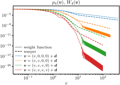
Figure 1: The weight function $W_{n}$ at order $n=4$ (plain lines) compared to its model function $p_{4}$ built by the projection technique (dashed lines), in the $E_{d}=\Gamma$ case. These functions are shown along several lines in the $\boldsymbol{v}$-space, parameterized by $v$ and starting at the point $\boldsymbol{d}=(2,2,2,2)$. Despite the simplistic form of the model function Eq. (29), it gives a good approximation in the low $v$ region and captures precisely the power law scaling of the long time tails.

III.4 Results

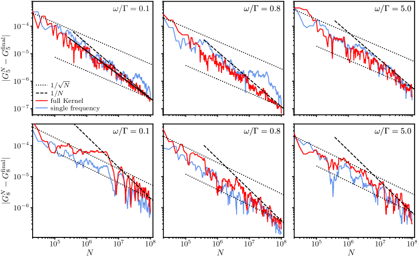
Figure 2: Convergence of the absolute error of the coefficients $G^{R}_{n}(\omega)$ calculated by QQMC with increasing number of function evaluations $N$. The full kernel calculation (red lines) is compared to the single frequency integration Eq. (21) (blue lines). Three frequencies $\omega/\Gamma=0.1,0.8$ and $5.0$ (columns) are shown at order $n=5$ (top row) and $n=8$ (bottom row). The model is the asymmetric one $E_{d}=\Gamma$. The scaling of the error is systematically better than or similar to $1/\sqrt{N}$ (dotted black lines), and is close to $1/N$ (dashed black lines) at small frequencies, reaching $1/N^{0.86}$ in the best case (black plain line in top left panel). For readability we show an upper bound to the error, see main text for details, and for the error estimation method.

Let us now apply QQMC to calculate the coefficients of the retarded Green function $G^{R}_{n}(\omega)$ of Eq. (1) in the perturbative expansion.

Figure 2 shows the convergence of the coefficients at order $n=5,8$ for three different frequencies $\omega/\Gamma=0.1,0.8$ and $5.0$. Specifically, we show the evolution of the absolute error with the number of function evaluations $N$. Each panel shows the two different methods outlined in the previous section – fixed single frequencies (blue curves) and full kernel method (red curves). The errors are estimated by taking the deviation of the value obtained for $G^{R}_{n}(\omega)$ after $N$ samples ($G^{N}_{n}$ in the figure) from the final value at $N=10^{8}$. The final value $G^{\textrm{final}}_{n}$ is taken to be the average of the last $10^{6}$ values. To improve readability, we show an upper bound to the error consisting of the maximum of a moving window around $N$ of fixed relative size ($4\%$ of $N$).

We focus first on the full kernel method. We observe that the convergence is systematically better than $1/\sqrt{N}$ (dotted line). It shows the best convergence in the top left panels ($\omega/\Gamma=0.1$ and $0.8$, $n=5$), where we observe convergence with a clear power law $1/N^{0.86}$ (black line). In the other panels ($n=8$ or $\omega/\Gamma=5$), the convergence is slower, but never worse than $1/\sqrt{N}$ (dotted lines). The slowdown at large order is expected, as it is more difficult for the model function to capture the details of the integrand at high dimension. Notice that at order $n=8$, the convergence is characterized by a slower rate for $N<3\cdot 10^{6}$ than for $N>3\cdot 10^{6}$. This separation in two regimes was already observed in Ref. 20.

As the single frequency method computes a single integral, it could be expected that the distribution of samples chosen by the projection technique is more adapted than the distribution used in the full kernel calculation. However, we see no significant improvement in using the single frequency integration: scalings are similar as well as absolute error values. The similarity between both methods convergences show that the weight function Eq. (22) is an efficient distribution for computing all frequencies at once, given that we approximate all distributions by a projection-based model function.

We now study the error as a function of frequency for different orders. The lower panel of Fig. 3 shows the absolute error in the self-energy coefficients $\Sigma_{n}(\omega)$ using the full kernel method and $N=10^{9}$ samples in the $E_{d}=0$ case. The self-energy is computed from the Green function series using Dyson’s equation $\Sigma(\omega)=g^{R}(\omega)^{-1}-G^{R}(\omega)^{-1}$. The error is estimated here by taking the standard deviation of the results of 10 randomized Sobol’ sequences. We see that the error is frequency dependent, with a minimum at $\omega=0$ reaching as low as a few $10^{-10}$ at large orders. The full kernel method is therefore well suited for low frequencies. The error does not change significantly as the order increases until $n=8$, but the coefficients decrease in absolute value by about an order of magnitude each 1–2 perturbation order (see Appendix B). Indeed, as the integration dimension increases, the relative error of the integral deteriorates. The top panels show some self-energy coefficients, with the error indicated as a shaded area. Order 6 (left) is well resolved for all frequencies with a significant signal. Order 10 (right) sees some deterioration due to the higher integration dimension, but accuracy is still good on a large range of frequencies. Only at high frequencies ($\omega>2\Gamma$) does the relative error become too large.

In brief, Ref. 20 showed that evaluating at a low discrepancy sequence of points makes it possible to compute single observables with an error decreasing faster than $1/\sqrt{N}$. Here, we establish that this also holds for dynamical quantities on a large range of frequencies, computed altogether with a single sampling. We also show that the kernel technique is well suited for that task, in particular at low frequencies.

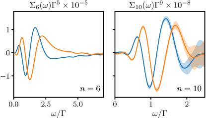
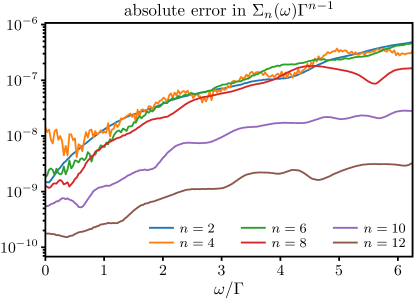
Figure 3: Self-energy series coefficients and absolute error, using the full kernel method on the $E_{d}=0$ impurity model. Top panels: self energy coefficient at order 6 (left) and 10 (right), blue is the real part, orange the imaginary part. Error bars are shown as a shaded area. Bottom panel: absolute error at different orders $n$. We used 10 shifted Sobol’ sequences of $10^{8}$ samples, and the error is the standard deviation between their results.

IV Resummation with Padé approximants

In the previous section, we described how to compute the frequency-dependent perturbation series coefficients $G^{R}_{n}(\omega)$ of the Green function. We showed that applying QQMC is efficient in a large frequency range, and we observed convergence scalings that outperform the $1/\sqrt{N}$ of conventional Monte Carlo. This was enabled by the automatic construction of a simple and computationally cheap – yet robust – model function. We can now resum these series to obtain physical quantities of interest. These can be compared with other numerical methods and we will perform a detailed comparison between QQMC and FTPS in later sections. In this section, we will discuss the series resummation of the Green function at values of the interaction $U$ beyond the radius of convergence.

There are several ways to perform resummation, with different performance characteristics. In Ref. 16, some of us designed a robust and general-purpose resummation technique based on conformal transforms; these were benchmarked on the Green function for an Anderson impurity system similar to the model of Section II. Instead of repeating that approach, we will perform resummation using Padé approximants, which are well-established method for analytical continuation [33, 19, 34, 35]. Here, we only provide a summary of relevant aspects and refer to the literature [22] for a detailed exposition. Note that in our analysis, we resum the perturbation series at each frequency $\omega$ independently; we will therefore generally suppress the $\omega$ dependence in the notation of this section.

The Padé approximant of type $[l/m]$ of a series is the unique rational function $P/Q$, with $P$ of degree at most $l$ and $Q$ of degree at most $m$, whose Taylor expansion at the origin matches the series up to the highest order possible [22]. When the series represents a function $f(U)$, such an approximant respects

$$P(U)-f(U)Q(U)=O(U^{l+m+1})$$ (35)

and generalizes the truncated Taylor series as an approximation of $f$ in the $U$ complex plane. However, unlike Taylor series, Padé approximants can capture the locations of poles and can be accurate beyond the convergence radius [22]. The choice of $l$ and $m$ is important for obtaining a good approximant. As the infinite $U$ limit is known $G^{R}(\omega)\rightarrow 0$, for $\omega\neq 0$, we impose the restriction $m\geq l$. For the purposes of this paper, we choose the simplest Padé that was sufficiently well matched with FTPS results presented below. Trying to find this Padé in a way that is independent of FTPS results is an involved process which we did not pursue here.

A recurrent issue with rational approximants is the occurrence of so-called defects or Froissart doublets [22, 36]. They are produced when $P/Q$ is close to a singular Padé approximant, in which a root of $P$ equals one of $Q$. The defect manifests as a localized zero-pole pair, which produces dramatic variations when the approximant is evaluated close-by, but has vanishing influence at long distance.

While defects are inevitable elements of Padé approximants, their locations are sensitive to the exact values of the coefficients $G^{R}_{n}$, so that noise may move them closer to or away from the point $U$ of interest. This causes extreme variance in the resummation of the series as $\omega$ varies and as the noise is changed (see Appendix C for an example). Such instabilities are evidence of the presence of a defect, and should be eliminated.

Some defects – but not all of them – are sensitive to the noise introduced by the integration method in both QQMC and traditional Monte Carlo. These may be statistically removed as follows. If each coefficient $G^{R}_{n}$ is known within an error bar $\delta G^{R}_{n}$, we assume it can be represented by a random variable following a normal probability law centered on $G^{R}_{n}$ and of standard deviation $\delta G^{R}_{n}$; we ignore potential correlations between orders. By sampling the series coefficients from this distribution (in practice we take 100 samples), we obtain as many Padé approximants, which we evaluate at the target $U$. This gives a population of resummed values at $U$, from which we take the median of the real or imaginary part as the final resummed result. The 15th and 85th percentiles are taken as the propagation of the coefficients error bar (these percentiles correspond to one sigma in the normal distribution). Note that these do not contain the error made by the resummation itself.

The population of resummed values do not form a Gaussian distribution, as would have been expected if using conformal transforms. Padé resummation is a non-linear process and the presence of defects close to the target $U$ brings outliers. For these reasons, median and percentiles are preferred over average and standard deviation. Nonetheless, the error bar obtained from percentiles still reflects the increased sensitivity of the Padé approximant in the series coefficients, in the presence of a defect near the target $U$.

Note that other defects may exist which are not susceptible to variations of the coefficients within error margins. These cannot be detected or eliminated statistically. Nevertheless, all the results in this article are resummed with a choice of $l$ and $m$ which shows no sign of such a defect in the vicinity of the target $U$.

Finally, we remark that by resampling the coefficients, we neglected the correlations between them. This makes it difficult to propagate error bars back in time domain after the Padé resummation.

V FTPS

Figure 4: Depiction of the MPS used for a impurity model with a small bath consisting of two sites. Note that the main idea of FTPS is to separate the spin-degrees of freedom (orbital-degrees of freedom in the multi-orbital case). Note that the sites one the left and on the right of the impurity does not correspond to the left or right lead as in Eq. 2 but represent the two different spin-degrees of freedom of the equilibrium bath.

In the recent years, Tensor Network (TN) methods – especially those based on Matrix Product States (MPS) – have been extensively applied to impurity problems [37, 38, 39, 40, 41, 42, 23, 43]. They allow for a systematically improvable representation of the impurity problem at all energy scales as well as well-developed approaches for real-time and imaginary time evolution. Here, we benchmark our QQMC results with those obtained from the Fork Tensor Product States (FTPS) impurity solver [23]. FTPS is a TN that is especially suited for multi-orbital impurity problems and it can be used to compute the impurity Green function on the real-frequency axis. This is achieved by a Density Matrix Renormalization Group (DMRG) [44, 45] calculation for the ground state followed by a time evolution in real time. For the single orbital model studied in this work, FTPS reduces to a Matrix Product State (MPS) as shown in Fig. 4 but we keep the term FTPS since certain details of the algorithm used to solve the impurity problem differ from standard MPS algorithms (see App. E).

A comparison of QQMC with FTPS is a fruitful endeavor since the approximations made in the two algorithms are drastically different. FTPS is non-perturbative and its accuracy can be systematically improved. However, it is wave-function based, and therefore solves a discretized version of the Anderson impurity model: a large but finite bath which consists of $N_{b}$ sites is used to represent the hybridization $\Delta^{R}(\omega)$ on a regular energy grid. The effect of such a discretization is that there exists a time $t_{\rm max}^{\rm FTPS}=\pi N_{b}/D$ after which the Green function shows finite size effects. Before that ($t<t_{\rm max}^{\rm FTPS}$), finite size effects are very small and the result behaves like the Green function of a model with the continuous bath. In this work we use $N_{b}=409$, so that $t_{\rm max}^{\rm FTPS}\approx 112/\Gamma$ in our parameters.

FTPS performs the computation in the so-called star geometry representation of the bath [24, 46, 47, 40]. In this representation, each bath degree of freedom is coupled directly to the impurity. Although this introduces long-range hopping terms in the Hamiltonian, this representation is superior for TN methods as it turns out [40].

We use FTPS to calculate the equilibrium zero-temperature retarded Green function $G^{R}(t)=-i\theta(t)\bra{\psi_{0}}\{c^{\phantom{\dagger}}_{0,\uparrow}(t),c_{0,\uparrow}^{\dagger}\}\ket{\psi_{0}}$ in real-time. To compute $G^{R}(t)$, FTPS first computes the ground state $\ket{\psi_{0}}$ using the Density Matrix Renormalization Group (DMRG), and time-evolves the states with an additional impurity electron/hole using the Time Dependent Variational Principle (TDVP) technique [48] in its two-site variant. TDVP can be considered as a set of coupled differential equations which are usually integrated in a certain order to obtain an algorithm very similar to DMRG [48]. FTPS uses a different integration order as discussed in App. E.

Using this approach, we perform the time evolution up to $t=40/\Gamma$ using a time step of $\Delta t=0.05/\Gamma$. To account for the finite maximum time we Fourier transform with a modified kernel $e^{i\omega t-\eta|t|}$, which generates a Lorentzian broadening of width $\eta$ in energy space. For the models studied in this work, the broadening is set to $0$ for spectral functions, since the Green functions in time decay rapidly enough (see Fig. 6). For the impurity self-energy, on the other hand, broadening is necessary because it is calculated from Dyson’s equation, which implies the non-interacting Green function calculated from the finite sized bath. This means that the non-interacting Green function consists of Dirac deltas with energy difference $\Delta\epsilon=\frac{2D}{N_{b}}$ which turns out to be rather large in our parameters: $\Delta\epsilon\approx 0.06\Gamma$ making some form of extrapolation necessary.

To obtain the $\eta\to 0$ self-energy, we calculate it for various broadenings $\eta$ and extrapolate each frequency point towards $\eta\to 0$ using a 4th order polynomial regression. We checked that this approach is consistent with the self energy obtained from the $\eta=0$ interacting Green function and the continuous non-interacting Green function. The latter yields worse self energies though, because Friedel oscillations that are barely visible in the interacting Green function are enhanced by the inversion in the Dyson equation.

The tensor network approximation used a truncated weight of $10^{-12}$ (sum of all squared discarded Schmidt values) and the maximal bond-dimensions were restricted to 300 for the link connecting the two impurity degrees of freedom and 200 for all other links. We checked that the results are converged with respect to larger bond dimensions and that they are converged in the time step $\Delta t$.

VI Comparing QQMC with FTPS

We now compare the results from the full kernel QQMC with those from FTPS on the Anderson impurity model in the Kondo regime. In this section, we show that the Green function perturbation series – calculated by QQMC – can produce results that match FTPS when resummed with a simple Padé approximant.

For each of the two cases, $E_{d}=0$ and $E_{d}=\Gamma$, the retarded Green function has been computed up to order $n=12$, and resummed in the frequency domain, as discussed above. We use $N=10^{9}$ function evaluations at each order; previous calculations some of the authors made using a Markov chain Monte Carlo [16] obtained less accurate results with 30 times more samples.

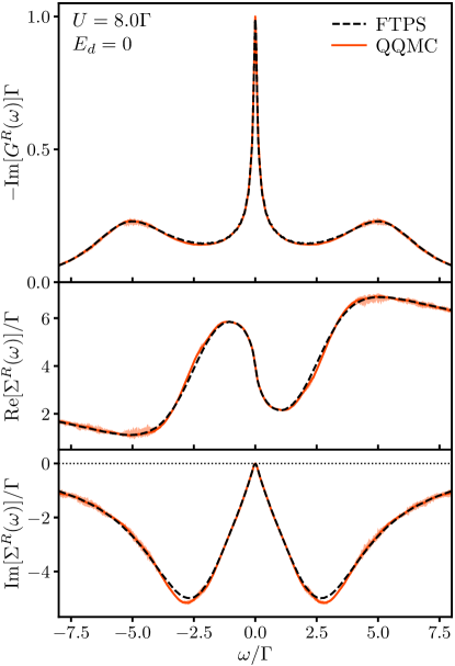
Figure 5: Comparison between QQMC result after resummation (plain line) and FTPS (dashed line), at $U=8\Gamma$ in the symmetric case $E_{d}=0$. Top panel: spectral function on the dot. Middle and bottom panels: real and imaginary parts of the associated self-energy. Shaded areas represent QQMC integration error estimate only (see main text). QQMC used $N=10^{9}$ function evaluations at each order.

VI.1 Symmetric model in frequency

Figure 5 shows results for the symmetric model ($E_{d}=0$) at $U=8\Gamma$, deep in the Kondo regime. In this model, due to particle-hole symmetry, the retarded Green function depends on $U^{2}$ instead of $U$. Its series is resummed using the $[2/4]$ Padé approximant (in the $U^{2}$ variable) at low frequencies $|\omega|<2\Gamma$, and $[2/3]$ at high frequencies. The high frequencies series decreases faster with order, so that high order coefficients are not resolved, and an approximant of lower rank is more accurate. The transition between the two Padés is progressive over a range $0.25\Gamma$.

The calculation of the coefficients $G_{n}^{R}(\omega)$ is subject to an error caused by the QQMC integration method, estimated as explained in Sec. III.4. In addition, the resummation of the series produces another error, which is difficult to estimate as it is linked to several factors (choice of Padé rank, finite perturbation series, defects). The error bars in Fig. 5 (shaded area) reflects the first error, propagated through the resummation, as explained in Sec. IV. Note that, as detailed in that section, these error bars reflect not only the precision of the series coefficients, but also the extreme sensitivity of the Padé approximant in these coefficients in the presence of a defect.

The density of states (top panel) displays the usual Kondo effect features: a thin Kondo peak at the Fermi level and lower and upper Hubbard bands centered around $\omega=\pm U/2$. The agreement between the two methods is very good, except at the tip of the Kondo peak. The Friedel sum rule [49] imposes that in the Kondo regime $-\imaginary[G^{R}(\omega=0)]=1/\Gamma$. It is respected by QQMC (plain line), but not by FTPS (dashed line) which lacks resolution at very low-frequencies due to its finite time limit.

The middle and lower panels show respectively the real and imaginary parts of the self-energy, where the agreement is also good. Deviations around $\omega=\pm 3\Gamma$ are attributed, by elimination of other possibilities, to the resummation error. We expect this to improve by increasing the number of orders. At larger frequencies $|\omega|>5\Gamma$, inaccuracies in the QQMC integration are the cause of the disagreement, as can be seen by the larger error bars. Although FTPS does not capture the low energy Green function perfectly, it still captures the Fermi liquid features, as it is much more precise in the low energy self-energy. Indeed, in our experience the $\eta$-extrapolation works better in the self-energy than in the spectral function. We speculate that this might be because the Kondo peak is sharper than the low-frequency self-energy, and therefore more difficult to extrapolate.

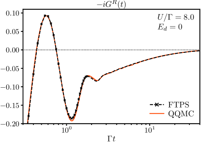
Figure 6: Retarded Green function in time domain, in the $E_{d}=0$ model at $U/\Gamma=8$. FTPS (dashed line and symbols) yields valid result only for a limited time, after which finite bath size effects occur. Symbols are shown only at small times for readability. QQMC (plain line) works directly in the thermodynamic limit, but may be less accurate at short times (high frequencies). Due to particle-hole symmetry, $G^{R}(t)$ is pure imaginary.

VI.2 Symmetric model in time

It is instructive to compare the Green function for the symmetric model in the time domain, as shown in Fig. 6. The Fourier transform of FTPS data suffer from an additional error due to its finite time extent. Hence, we show here the FTPS data before $\eta$-extrapolation (dashed line and symbols, symbols are shown only at small times for readability). The QQMC data (plain orange line) is the same as in Fig. 5 after Fourier transformation. Error bars have not been propagated through this Fourier transform, as it would require knowledge of noise correlations between frequencies, which has been lost during the Padé resummation.

The QQMC result shows good agreement with FTPS, concerning the large oscillations and the long time decay rate, and out-range FTPS at long times (note the logarithmic time scale). However, discrepancies can be seen in the high frequency features. The difference in the two first oscillations is linked to the mismatch in Fig. 5 around $\omega\approx\pm 3\Gamma$, already discussed above. The small mismatch in the long time oscillations ($\Gamma t>3$) is connected to frequencies near the bandwidth $\omega\approx\pm D$, where QQMC has lower resolution when calculating coefficients (see Fig. 3).

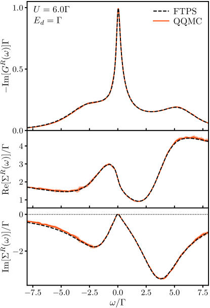
Figure 7: Comparison between QQMC result after resummation (plain line) and FTPS (dashed line), at $U=6\Gamma$ in the asymmetric case. Top panel: spectral function on the dot. Middle and bottom panels: real and imaginary parts of the associated self-energy. Shaded areas represent QQMC integration error estimation.

VI.3 Asymmetric model

Finally, we consider the asymmetric model ($E_{d}=\Gamma$) at $U=6\Gamma$, for which the comparison in the frequency domain is shown in Fig. 7. The resummation was done with the $[6/6]$ Padé approximant at low frequencies $|\omega|<4\Gamma$, and $[4/4]$ at high frequencies. The same progressive transition has been used as in the symmetric model.

In spite of the lower interaction, we still recognize the main features of the Kondo regime in the density of states (upper panel): the Kondo peak at the Fermi level and an upper and lower Hubbard bands at $\omega\approx E_{d}\pm U/2$. As the Kondo peak is broader than in Fig. 5, it is expected to be better captured by FTPS than in the particule-hole symmetric case. The real and imaginary parts of the self-energy (middle and lower panels) show an overall good agreement. As in the particle-hole symmetric case, large frequencies are more noisy in the QQMC result, due to larger relative errors when calculating coefficients.

VII Conclusion

Using the recently developed QQMC method based on low-discrepancy integration of Ref. 20, we computed a full real-time Green function perturbation series in an interacting quantum system. We compared two different algorithms that adapt the kernel-based technique of Ref. 17, originally designed with a Markov chain Monte Carlo integration. The first one computes the kernel at a given frequency as a single integral, while the second computes its whole time dependence at once using the same sampling of the integration space. We optimize the QQMC integration by using a warping technique which introduces information on the integrand in a problem-independent way.

For both methods, switching from traditional Monte Carlo to the novel QQMC brought an important speedup in the calculation of the Green function perturbation series. This is caused by an improved convergence, the error scaling in the best cases as $1/N^{0.86}$, with $N$ the number of samples. In practice, we typically gain 2-3 orders of magnitude in precision. More importantly, the switch to quasi-Monte Carlo opened up the possibility to further improve the convergence rate. Indeed, unlike with Monte Carlo, this rate depends on the smoothness of the integrand, which could be improved by more advanced warpings.

The full kernel method turns out to be superior to the single frequency method, strengthening the idea that a single sampling distribution can be used efficiently to compute a continuum of correlators. Nevertheless, more advanced warpings could change the ratio of performance in the future.

Applying this technique to a zero-temperature Anderson impurity model, and after resummation of the Green function series using Padé approximants, we compared the full kernel QQMC result to the non-perturbative FTPS technique. This comparison brought an overall very good agreement between the two very different methods. The observed discrepancies can be linked to limitations in both algorithms: the low frequencies are better resolved by the kernel method due to the long time limitation of FTPS, but the high frequencies are more accurate in the FTPS results, probably due to biases introduced by the resummation and integration noise.

From the FTPS viewpoint, this comparison showed that long time Green functions results (up to $t=40/\Gamma$) using only time evolution, as well as low frequency self-energies are reliable.

The QQMC technique is versatile and can easily be adapted to more complex systems such as multi-band or multi-orbital impurity models, or lattice models, although performance is still an open question. In addition, the integration algorithm is highly automatic, thanks to the projection-based technique for building tailor-made warpings.

Further developments can be made to improve the current algorithm for computing the Green function perturbation series. First, high frequency noise could be reduced by adapting QQMC to computing the $L$ kernel, as defined in Ref. 17. Finally, as with the calculation of a single quantity, building warpings that capture more features of the integrand would allow faster convergence, potentially allowing access to higher perturbation orders.

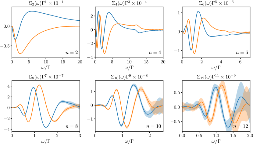
Figure 8: Perturbation series for $\Sigma(\omega)$ in the symmetric model ($E_{d}=0$). Orders $n=2,4,\ldots,12$ are shown in reading order from the top left. The real part is in blue, the imaginary in orange. The estimated error is shown as a shaded area.

Appendix A Equal-time Green function: a time splitting implementation

As mentioned in Sec. III.1, care needs to be taken when evaluating the Wick determinant, since the Green functions $g^{T}(t,t^{\prime}),g^{\widetilde{T}}(t,t^{\prime})$ have a discontinuity at $t=t^{\prime}$. Here we elaborate on how to correctly addressed this problem.

First, the Green functions $g(U_{k},U_{k})$ along the diagonal of the determinant correspond to Wick contraction of Fermion operators within the interacting Hamiltonian $H_{I}$. These Green functions are replaced by $g^{<}(u_{k},u_{k})-i\alpha$. The choice $g^{<}$ reflects the correct operator ordering $\sim c^{\dagger}c$ for each spin block of $H_{I}$; the $-i\alpha$ term accounts for the quadratic shift.

Secondly, we encounter the situation where times $u=v$ in Green functions, which correspond to Wick contractions between operators between two Hamiltonians $H_{I}(u)H_{I}(v)$. The $u\to v$ limit is on the edge of the integration region in the time ordered perturbative expansion and has measure zero. For numerical evaluation of the integral, however, we want to include this boundary and define it such that the $u\to v$ limit is smooth.

A simple way to implement this smooth limit is to impose a “time-splitting” procedure. Specifically, each time appearing in Eq. (6) is associated with an additional splitting index, which can be appended to the combined index

$$X =(t,a)\rightarrow(t,a,0),$$ (36)

$$X^{\prime} =(t^{\prime},b)\rightarrow(t^{\prime},b,0),$$ (37)

$$U_{k} =(u_{k},a_{k})\rightarrow(u_{k},a_{k},k).$$ (38)

The definition of the non-interacting Green function $g$ is adjusted so that for any $A=(u,a,s)$ and $B=(v,b,r)$,

$$g(A,B)=\lim_{\epsilon\rightarrow 0}g^{ab}(u+s\epsilon,v+r\epsilon).$$ (39)

In practice, the order of $A$ and $B$ on the Keldysh contour is determined: first, by the Keldysh indices $a,b$; second, if $a=b$, by the times $u,v$; third, if $a=b$ and $u=v$, by the splittings $s,r$. Thus, $A=B$ if and only if Keldysh indices, times and splittings are equal. The Green function is then unambiguously

$$g(A,B)=\begin{cases}g^{<}(u,v),&\mathrm{if}\leavevmode\nobreak\ A\leq B,\\ g^{>}(u,v),&\mathrm{otherwise}.\end{cases}$$ (40)

Appendix B Perturbation series of the self-energy

The perturbation series for the self-energy in the symmetric model ($E_{d}=0$) is shown up to order 12 in Fig. 8. The real part is in blue, the imaginary in orange. The estimated error is shown as a shaded area. In this model, even orders are zero due to the particle-hole symmetry.

The self-energy coefficients lose about one order of magnitude in amplitude every 1–2 perturbation orders, providing good convergence properties. To benefit from this, we need to compute coefficients with an amplitude as low as $10^{-9}$ at order 12.

Appendix C Susceptibility of some Froissart doublets to noise

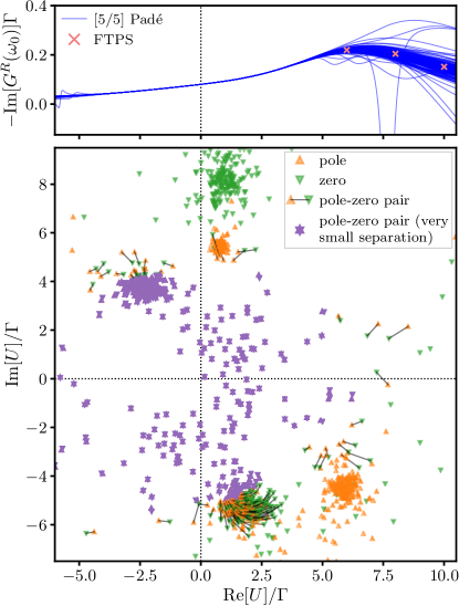
Figure 9: Distribution of poles, zeros, and pole–zero pairs of the $[5/5]$ Padé approximant of a noisy series (bottom panel) and corresponding evaluation of the approximant on the real axis (top panel). The series is $G^{R}_{n}(\omega_{0})$ for the asymmetric model ($E_{d}=\Gamma$) with addition of different realizations of a Gaussian noise compatible with QQMC error bars, with $\omega_{0}=-2.58\Gamma$. Poles are orange triangles pointing up, zeros are green triangles pointing down. Within each realization of noise, pole–zero pairs which are close (separation $\delta<\Gamma$) are shown with a black line joining them. Purple symbols shows pairs with a very small separation ($\delta<0.2\Gamma$, overlapping symbols), a clear indication of a defect. These are spread out in a large region of the complex plane. Occurrences near the real axis are not rare, but affect much more the evaluation of the approximant (blue lines in top panel) in the range $\real[U]/\Gamma>4$ than $\real[U]/\Gamma<4$.

Froissart doublets or defects are known features of Padé approximants formed of a pole and a zero in the complex plane, separated by a small distance $\delta$. These defects strongly disrupt the expected behavior of the approximant in their vicinity, but have a vanishing effect $\sim\delta/L$ at long distance $L$. The location of defects can be very sensitive to accuracy on the coefficients of the series. This can be a problem, if such defects appear close to a region of interest. In this appendix, we look at the influence of uncertainty on the coefficients $G^{R}_{n}(\omega_{0})$, on the location of defects and the evaluation of the Padé approximant. For in-depth mathematical studies of the phenomenon on simpler series, we refer to the literature [52, 53].

We consider the asymmetric model ($E_{d}=\Gamma$) and the $[5/5]$ Padé approximant for a given frequency $\omega_{0}=-2.58\Gamma$. We generate a Gaussian noise in the series $G^{R}_{n}(\omega_{0})$ that is compatible with the QQMC error bars, ignoring correlations between coefficients.

The location of the poles and zeros of the $[5/5]$ Padé approximant using 200 realizations of this noise are displayed in Fig. 9 (lower panel). Poles are shown as orange triangles pointing up, and zeros as green triangles pointing down. Poles and zeros that are suspected to be part of a defect are displayed differently. If a pole and a zero of the same Padé are close enough so that their symbols overlap($\delta<0.2\Gamma$) , they are drawn in purple. Otherwise, if their separation is $\delta<\Gamma$, they are linked together by a black line.

A $[5/5]$ Padé approximant has 5 poles and 5 zeros in the complex plane. We can locate them in Fig. 9. We notice immediately two poles ($U/\Gamma\approx 6-4i$ and $U/\Gamma\approx 1+5.5i$) and a zero ($U/\Gamma\approx 1.5+8i$) that are stable. In addition, two other stable structures (at $U/\Gamma\approx 2-5i$ and $U/\Gamma\approx-2.5+4i$) are formed of pole–zero pairs, and are probably defects. These are far from the real axis so they do not affect strongly the evaluation of the Padé approximant there. More interesting is the last pair that spans a large region of the complex plane, in particular many occurrences (but not all) have a modulus $<3/\Gamma$. This defect is problematic as it may appear very close to the real axis. Finally, a last zero spreads mostly out of the shown area, at very large moduli.

The top panel of Fig. 9 shows the spectral function (beam of blue lines), evaluated on the real $U$ axis from the above-mentioned Padé approximants, for each realization of noise. Notice the stability of the evaluation for $|\real[U]/\Gamma|<4$, even though several defects appear close to the real axis in this range. However, these defects have an extremely small separation $\delta\sim 10^{-5}\Gamma$ compared to their distance from the real axis $L\sim 10^{-1}\Gamma$. As $U$ increases, the beam of lines spread further more but stays consistent with FTPS calculations (red crosses). However, a dozen among all 200 lines have dramatic variations, inconsistent with the other lines or with FTPS. These are caused by the defects observed close to the real axis in the range $4<\real[U]/\Gamma<8$. These defects have a larger separation $\delta\sim\Gamma$, and therefore a higher probability to be within a few $\delta$ from the real axis. As one can see, the defect causing wild variations of the density of states has a strong probability to lie within a distance $<3\Gamma$ of the origin, where it is observed not to affect evaluation on the real axis. We use this probability in Sec. IV to eliminate the effect of this defect.

The analytical structure of Padé approximants possesses features that are more or less stable to perturbations in the Taylor coefficients. We observe that some defects are extremely unstable and can vary wildly in location, whereas some poles and zeros are stable.

Appendix D Empirical convergence of Padé approximants

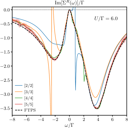
Figure 10: Convergence of the self-energy (imaginary part) using $[m/m]$ Padé resummation of the Green function with increasing $m=2,\dots,5$ (plain lines). The model is the $E_{d}=\Gamma$ one at $U=6\Gamma$. Notwithstanding abrupt variations caused by defects in Padé approximants, the sequence converges toward a result consistent with the FTPS computation (dashed line). For clarity, only the error bar of $m=5$ is shown (pale red area). $m=2$ and $3$ errors are smaller than the line width, $m=4$ error is of the same magnitude as $m=5$.

The convergence of a sequence of $[l/m]$ Padé approximants with increasing $l$ and $m$ is the subject of intense mathematical research. No known result allows us to prove that the approximants we consider in this work are part of a uniformly converging sequence of functions.

However, we observe that several sequences of Padé approximants empirically converge, ignoring spurious peaks caused by defects. Such a sequence is represented in Fig. 10. The figure shows the imaginary part of the self-energy at $U=6\Gamma$ obtained by resummation of the series $G_{n}^{R}(\omega)$ using $[m/m]$ Padé approximants (plain lines). We show $m=2,\ldots,5$; $m=6$ is not displayed for clarity, as it is difficult to distinguish from $m=5$. The resummation follows the same statistical treatment as described in Sec. IV, to remove the least stable defects. Some defects nevertheless survived, as can be seen for instance around $\omega=-2.5\Gamma$ and $\omega=0.8\Gamma$, in the $[3/3]$ and $[2/2]$ Padé approximants respectively (strong variations in the self-energy are correlated to strong variations in the Green function). Ignoring these extreme variations, the successive approximants seem to converge toward a result that is consistent with the FTPS calculation (dashed line).

It is interesting to note that the $[5/5]$ (as well as $[6/6]$) approximant seems free of defects, whereas lower order approximants are not. It is possible that the larger uncertainty in the evaluation of large order $G^{R}_{n}(\omega)$ make defects more susceptible to our statistical treatment, and as a result easier to erase.

Figure 11: Depiction of the TDVP sweeping order the time step to time evolve from time $t$ to $t+\Delta t$. This picture is the equivalent of Eq. 43 and shows the terms that are being integrated on the left. The steps shown start in the middle of the MPS (on the impurity site) and move outwards the spin-up bath (see also Fig. 4). Yellow dots are the sites that are updated in each step. As usual, two-site updates are in forward direction (negative exponent) while single-site updates are in backward direction (positive exponent). Note that this is quite different from the usual TDVP given by Eq. 43 which would start with the middle term ($P_{12}$) move upwards, but would do steps (1–3) in a different order. See also Ref. 54 for more details.

Appendix E TDVP Time Evolution

The main idea behind the Time Dependent Variational Principle (TDVP) is to find the best possible representation of time evolved states represented as MPS. To do so it solves a modified Schrödinger equation in which the right-hand side is changed: $H|\psi\rangle\to PH|\psi\rangle$. The projection operator $P$ projects onto the so-called tangent space of the current MPS $|\psi\rangle$ and keeps the time integration within the manifold spanned by $|\psi\rangle$ [48]. In the two-site variant of TDVP, $P$ is given by [48]:

$$P=\sum_{i=1}^{N-1}P_{i,i+1}-\sum_{i=2}^{N-1}P_{i},$$ (41)

with so-called two-site projection operators $P_{i,i+1}$ and single-site projectors $P_{i}$. The exact form of these operators is of no relevance here and can be found in Ref. [48]. Their sole purpose is to solve the Schrödinger equation only in the subspace spanned by the MPS. The two-site projectors result in the usual forward time propagation, while the single site projectors stem from the gauge degree of freedom of the MPS and make sure that entries are not time evolved twice. This is achieved via a backwards time evolution with opposite sign to the two-site projectors, see also Eq. 42. Importantly this means that the formal solution of the modified Schrödinger equation is given by:

$$|\psi(t+\Delta t)\rangle=e^{-i\left(\sum_{i=1}^{N-1}P_{i,i+1}-\sum_{i=2}^{N-1}P_{i}\right)H\Delta t}|\psi(t)\rangle.$$ (42)

Every single term (e.g. $e^{-iP_{i,i+1}H\Delta t}$ or $e^{iP_{i+1}H\Delta t}$) can easily be integrated nearly exactly using Krylov matrix exponentiation but the whole sum is far too complicated to deal with at once. Hence a second order trotter decomposition is used to split the whole exponential into manageable parts usually starting with the two-site term containing $P_{1,2}$ then $P_{2}$, next $P_{2,3}$ etc.:

$$e^{-i\left(\sum_{i=1}^{N-1}P_{i,i+1}-\sum_{i=2}^{N-1}P_{i}\right)H\Delta t}\approx e^{-iP_{1,2}H\Delta t/2}\cdot e^{-i\left(\sum_{i=2}^{N-1}P_{i,i+1}-\sum_{i=2}^{N-1}P_{i}\right)H\Delta t}\cdot e^{-iP_{1,2}H\Delta t/2}$$

$$\approx e^{-iP_{1,2}H\Delta t/2}\cdot e^{+iP_{2}H\Delta t}\cdot e^{-i\left(\sum_{i=2}^{N-1}P_{i,i+1}-\sum_{i=3}^{N-1}P_{i}\right)H\Delta t}\cdot e^{+iP_{2}H\Delta t}\cdot e^{-iP_{1,2}H\Delta t/2}$$

$$\approx\cdots\approx\left(\prod_{i=1}^{N-2}e^{-iP_{i,i+1}H\Delta t/2}\cdot e^{+iP_{i+1}H\Delta t/2}\right)e^{-iP_{N-1,N}H\Delta t}\left(\prod_{i=N-2}^{1}e^{-iP_{i,i+1}H\Delta t/2}\cdot e^{+iP_{i+1}H\Delta t/2}\right).$$ (43)

Note that the indices of the products above are defined such that the rightmost as well as the leftmost term is the one that contains $P_{1,2}$. Applying each operator in the order indicated by Eq. 43 results in the usual TDVP integration scheme as proposed in Ref. 48. It is worth noting that starting the trotterization with the $P_{1,2}$-term is a convenient choice since it results in an algorithm very similar to DMRG but there is nothing preventing one from starting with any other term.
 
In fact here, we use a different integration order as shown in Fig. 11 which is the pictorial equivalent of Eq. 43. We start at one of the center sites which is the impurity where the creation/annihilation operator is applied (sites $4$ and $5$ in Fig. 11), sweeping right, jumping back to the center and sweeping left. Again, since we use a second order breakup, all steps have to be applied twice in an order resulting from repeated second order trotter breakups similar to Eq. 43.

We choose this different integration order because a direct application of Eq. 43 would lead to large but unnecessary errors, especially for large values of $\Delta t$. If one were to use exclusively Eq. 43, the first few time steps would have to work with an inadequate basis, because after the application of the creation (annihilation) operator the remaining basis consists only of states in which the impurity is completely full (empty). It is known that TDVP is very susceptible to a too small number of basis states (bond dimension) [55] and therefore this inadequate basis leads to large errors in the first few time steps. The scheme shown in Fig. 11 does not have this problem, since it can produce the missing basis states in the very first step (the $P_{4,5}$-term in Fig. 11). We stress that the new scheme is important only for the first few time steps. Eq.43 is perfectly adequate, although not better than the scheme of Fig.11, for larger times. Another reason for using this integration order is that it is easier to generalize to multi-orbital problems which is the main purpose of the FTPS tensor network.

References

- Gross and Bloch [2017] C. Gross and I. Bloch, Quantum simulations with ultracold atoms in optical lattices, Science 357, 995 (2017).
- Bernien et al. [2017] H. Bernien, S. Schwartz, A. Keesling, H. Levine, A. Omran, H. Pichler, S. Choi, A. S. Zibrov, M. Endres, M. Greiner, V. Vuletić, and M. D. Lukin, Probing many-body dynamics on a 51-atom quantum simulator, Nature 551, 579 (2017), arXiv:1707.04344 .
- Blatt and Roos [2012] R. Blatt and C. F. Roos, Quantum simulations with trapped ions, Nature Phys 8, 277 (2012).
- Goldhaber-Gordon et al. [1998a] D. Goldhaber-Gordon, H. Shtrikman, D. Mahalu, D. Abusch-Magder, U. Meirav, and M. A. Kastner, Kondo effect in a single-electron transistor, Nature 391, 156 (1998a).
- Goldhaber-Gordon et al. [1998b] D. Goldhaber-Gordon, J. Göres, M. A. Kastner, H. Shtrikman, D. Mahalu, and U. Meirav, From the Kondo regime to the mixed-valence regime in a single-electron transistor, Phys. Rev. Lett. 81, 5225 (1998b).
- Cronenwett et al. [1998] S. M. Cronenwett, T. H. Oosterkamp, and L. P. Kouwenhoven, A tunable Kondo effect in quantum dots, Science 281, 540 (1998).
- Iftikhar et al. [2018] Z. Iftikhar, A. Anthore, A. K. Mitchell, F. D. Parmentier, U. Gennser, A. Ouerghi, A. Cavanna, C. Mora, P. Simon, and F. Pierre, Tunable quantum criticality and super-ballistic transport in a “charge” Kondo circuit, Science 360, 1315 (2018).
- Prokof’ev and Svistunov [1998] N. V. Prokof’ev and B. V. Svistunov, Polaron problem by diagrammatic quantum Monte Carlo, Phys. Rev. Lett. 81, 2514 (1998), arXiv:cond-mat/9804097 .
- Prokof’ev and Svistunov [2008] N. V. Prokof’ev and B. V. Svistunov, Bold diagrammatic Monte Carlo: A generic sign-problem tolerant technique for polaron models and possibly interacting many-body problems, Phys. Rev. B 77, 125101 (2008), arXiv:0801.0911 .
- Mishchenko et al. [2001] A. S. Mishchenko, N. V. Prokof’ev, B. V. Svistunov, and A. Sakamoto, Comprehensive study of Fröhlich polaron, in Excitonic Processes in Condensed Matter (WORLD SCIENTIFIC, 2001) pp. 372–375, cond-mat/9910025 .
- Van Houcke et al. [2012] K. Van Houcke, F. Werner, E. Kozik, N. Prokof’ev, B. Svistunov, M. J. H. Ku, A. T. Sommer, L. W. Cheuk, A. Schirotzek, and M. W. Zwierlein, Feynman diagrams versus Fermi-gas Feynman emulator, Nature Phys 8, 366 (2012), arXiv:1110.3747 .
- Profumo et al. [2015] R. E. V. Profumo, C. Groth, L. Messio, O. Parcollet, and X. Waintal, Quantum Monte Carlo for correlated out-of-equilibrium nanoelectronic devices, Phys. Rev. B 91, 245154 (2015), arXiv:1504.02132 .
- Wu et al. [2017] W. Wu, M. Ferrero, A. Georges, and E. Kozik, Controlling Feynman diagrammatic expansions: Physical nature of the pseudogap in the two-dimensional Hubbard model, Phys. Rev. B 96, 041105 (2017), arXiv:1608.08402 .
- Rossi [2017] R. Rossi, Determinant diagrammatic Monte Carlo algorithm in the thermodynamic limit, Phys. Rev. Lett. 119, 045701 (2017), arXiv:1612.05184 .
- Chen and Haule [2019] K. Chen and K. Haule, A combined variational and diagrammatic quantum Monte Carlo approach to the many-electron problem, Nat Commun 10, 3725 (2019), arXiv:1809.04651 .
- Bertrand et al. [2019a] C. Bertrand, S. Florens, O. Parcollet, and X. Waintal, Reconstructing nonequilibrium regimes of quantum many-body systems from the analytical structure of perturbative expansions, Phys. Rev. X 9, 041008 (2019a), arXiv:1903.11646 .
- Bertrand et al. [2019b] C. Bertrand, O. Parcollet, A. Maillard, and X. Waintal, Quantum Monte Carlo algorithm for out-of-equilibrium Green’s functions at long times, Phys. Rev. B 100, 125129 (2019b), arXiv:1903.11636 .
- Moutenet et al. [2019] A. Moutenet, P. Seth, M. Ferrero, and O. Parcollet, Cancellation of vacuum diagrams and the long-time limit in out-of-equilibrium diagrammatic quantum Monte Carlo, Phys. Rev. B 100, 085125 (2019), arXiv:1904.11969 .
- Rossi et al. [2020] R. Rossi, F. Šimkovic, and M. Ferrero, Renormalized perturbation theory at large expansion orders, EPL (Europhysics Letters) 132, 11001 (2020), arXiv:2001.09133 .
- Maček et al. [2020] M. Maček, P. T. Dumitrescu, C. Bertrand, B. Triggs, O. Parcollet, and X. Waintal, Quantum quasi-Monte Carlo technique for many-body perturbative expansions, Phys. Rev. Lett. 125, 047702 (2020).
- Calabrese and Cardy [2005] P. Calabrese and J. Cardy, Evolution of entanglement entropy in one-dimensional systems, Journal of Statistical Mechanics: Theory and Experiment 2005, P04010 (2005).
- Baker and Graves-Morris [1996] G. Baker and P. Graves-Morris, Padé Approximants, Encyclopedia of Mathematics and its Applications, Vol. 59 (Cambridge University Press, 1996).
- Bauernfeind et al. [2017] D. Bauernfeind, M. Zingl, R. Triebl, M. Aichhorn, and H. G. Evertz, Fork tensor-product states: Efficient multiorbital real-time DMFT solver, Phys. Rev. X 7, 031013 (2017).
- Anderson [1961] P. W. Anderson, Localized magnetic states in metals, Phys. Rev. 124, 41 (1961).
- Rubtsov and Lichtenstein [2004] A. N. Rubtsov and A. I. Lichtenstein, Continuous-time quantum Monte Carlo method for fermions: Beyond auxiliary field framework, Journal of Experimental and Theoretical Physics Letters 80, 61 (2004).
- Rammer [2007] J. Rammer, Quantum Field Theory of Non-equilibrium States (Cambridge University Press, 2007).
- Lepage [1978] G. P. Lepage, A new algorithm for adaptive multidimensional integration, Journal of Computational Physics 27, 192 (1978).
- Lepage [1980] G. P. Lepage, VEGAS - an adaptive multi-dimensional integration program, Tech. Rep. CLNS-447 (Cornell Univ. Lab. Nucl. Stud., Ithaca, NY, 1980).
- Dick et al. [2013] J. Dick, F. Y. Kuo, and I. H. Sloan, High-dimensional integration: The quasi-Monte Carlo way, Acta Numerica 22, 133 (2013).
- Nuyens [2014] D. Nuyens, The construction of good lattice rules and polynomial lattice rules, in Uniform Distribution and Quasi-Monte Carlo Methods (DE GRUYTER, 2014) pp. 223–256, arXiv:1308.3601 [math.NA] .
- Dick and Pillichshammer [2010] J. Dick and F. Pillichshammer, Digital Nets and Sequences: Discrepancy Theory and Quasi-Monte Carlo Integration (Cambridge University Press, 2010).
- L’Ecuyer [2018] P. L’Ecuyer, Randomized quasi-Monte Carlo: An introduction for practitioners, in Monte Carlo and Quasi-Monte Carlo Methods, edited by A. B. Owen and P. W. Glynn (Springer International Publishing, Cham, 2018) pp. 29–52.
- Hunter and Baker [1979] D. L. Hunter and G. A. Baker, Methods of series analysis. III. Integral approximant methods, Physical Review B 19, 3808 (1979).
- Pavlyukh [2017] Y. Pavlyukh, Padé resummation of many-body perturbation theories, Scientific Reports 7, 10.1038/s41598-017-00355-w (2017).
- Šimkovic and Kozik [2019] F. Šimkovic and E. Kozik, Determinant Monte Carlo for irreducible Feynman diagrams in the strongly correlated regime, Phys. Rev. B 100, 121102 (2019).
- Stahl [1998] H. Stahl, Spurious poles in Padé approximation, Journal of Computational and Applied Mathematics 99, 511 (1998), proceeding of the VIIIth Symposium on Orthogonal Polynomials and Thier Application.
- Jeckelmann [2002] E. Jeckelmann, Dynamical density-matrix renormalization-group method, Phys. Rev. B 66, 045114 (2002).
- García et al. [2004] D. J. García, K. Hallberg, and M. J. Rozenberg, Dynamical mean field theory with the density matrix renormalization group, Phys. Rev. Lett. 93, 246403 (2004).
- Ganahl et al. [2015] M. Ganahl, M. Aichhorn, H. G. Evertz, P. Thunström, K. Held, and F. Verstraete, Efficient dmft impurity solver using real-time dynamics with matrix product states, Phys. Rev. B 92, 155132 (2015).
- Wolf et al. [2014a] F. A. Wolf, I. P. McCulloch, and U. Schollwöck, Solving nonequilibrium dynamical mean-field theory using matrix product states, Phys. Rev. B 90, 235131 (2014a).
- Wolf et al. [2014b] F. A. Wolf, I. P. McCulloch, O. Parcollet, and U. Schollwöck, Chebyshev matrix product state impurity solver for dynamical mean-field theory, Phys. Rev. B 90, 115124 (2014b).
- Wolf et al. [2015] F. A. Wolf, A. Go, I. P. McCulloch, A. J. Millis, and U. Schollwöck, Imaginary-time matrix product state impurity solver for dynamical mean-field theory, Phys. Rev. X 5, 041032 (2015).
- Linden et al. [2020] N.-O. Linden, M. Zingl, C. Hubig, O. Parcollet, and U. Schollwöck, Imaginary-time matrix product state impurity solver in a real material calculation: Spin-orbit coupling in , Phys. Rev. B 101, 041101 (2020).
- White [1992] S. R. White, Density matrix formulation for quantum renormalization groups, Phys. Rev. Lett. 69, 2863 (1992).
- Schollwöck [2011] U. Schollwöck, The density-matrix renormalization group in the age of matrix product states, Annals of Physics 326, 96 (2011), january 2011 Special Issue, arXiv:1008.3477 .
- Bulla et al. [2008] R. Bulla, T. A. Costi, and T. Pruschke, Numerical renormalization group method for quantum impurity systems, Rev. Mod. Phys. 80, 395 (2008).
- Caffarel and Krauth [1994] M. Caffarel and W. Krauth, Exact diagonalization approach to correlated fermions in infinite dimensions: Mott transition and superconductivity, Physical Review Letters 72, 1545 (1994).
- Haegeman et al. [2016] J. Haegeman, C. Lubich, I. Oseledets, B. Vandereycken, and F. Verstraete, Unifying time evolution and optimization with matrix product states, Phys. Rev. B 94, 165116 (2016).
- Hewson [1993] A. C. Hewson, The Kondo Problem to Heavy Fermions, Cambridge Studies in Magnetism (Cambridge University Press, 1993).
- Parcollet et al. [2015] O. Parcollet, M. Ferrero, T. Ayral, H. Hafermann, I. Krivenko, L. Messio, and P. Seth, TRIQS: A toolbox for research on interacting quantum systems, Computer Physics Communications 196, 398 (2015).
- Kuo and Nuyens [2016] F. Y. Kuo and D. Nuyens, Application of quasi-Monte Carlo methods to elliptic PDEs with random diffusion coefficients: A survey of analysis and implementation, Found Comput Math 16, 1631 (2016).
- Gilewicz and Pindor [1997] J. Gilewicz and M. Pindor, Padé approximants and noise: A case of geometric series, Journal of Computational and Applied Mathematics 87, 199 (1997).
- Gilewicz and Pindor [1999] J. Gilewicz and M. Pindor, Padé approximants and noise: rational functions, Journal of Computational and Applied Mathematics 105, 285 (1999).
- Bauernfeind and Aichhorn [2020] D. Bauernfeind and M. Aichhorn, Time Dependent Variational Principle for Tree Tensor Networks, SciPost Phys. 8, 24 (2020).
- Yang and White [2020] M. Yang and S. R. White, Time-dependent variational principle with ancillary krylov subspace, Phys. Rev. B 102, 094315 (2020).