A medium-resolution spectrum of the exoplanet HIP 65426 b

Medium-resolution integral-field spectrographs (IFS) coupled with adaptive-optics such as Keck/OSIRIS, VLT/MUSE, or SINFONI are appearing as a new avenue for enhancing the detection and characterization capabilities of young, gas giant exoplanets at large heliocentric distances ($>$5 au). We analyzed K-band VLT/SINFONI medium-resolution ($R_{\lambda}\sim$ 5577) observations of the young giant exoplanet HIP 65426 b. Our dedicated IFS data analysis toolkit (TExTRIS) optimied the cube building, star registration, and allowed for the extraction of the planet spectrum. A Bayesian inference with the nested sampling algorithm coupled with the self-consistent forward atmospheric models BT-SETTL15 and Exo-REM using the ForMoSA tool yields $\mathrm{T_{eff}}$=1560$\pm 100$ K, log(g)$\leq$4.40  dex, [M/H]=$0.05^{+0.24}_{-0.22}$ dex, and an upper limit on the C/O ratio ($\leq$0.55). The object is also re-detected with the so-called “molecular mapping” technique. The technique yields consistent atmospheric parameters, but the loss of the planet pseudo-continuum in the process degrades or modifies the constraints on these parameters. The solar to sub-solar C/O ratio suggests an enrichment by solids at formation if the planet was formed beyond the water snowline ($\geq$20 au) by core-accretion. However, a formation by gravitational instability can not be ruled out. The metallicity is compatible with the bulk enrichment of massive Jovian planets from the Bern planet population models. Finally, we measure a radial velocity of 26$\pm$15   km s^-1  compatible with our revised measurement on the star. This is the fourth imaged exoplanet for which a radial velocity can be evaluated, illustrating the potential of such observations for assessing the coevolution of imaged systems belonging to star forming regions, such as HIP 65426.

1 Introduction

Table 1: Observing log

Date	UTC Time	Instrument	Setup	DIT	Nexp	$\mu$	seeing	$<$Strehl$>$	$\Delta\pi$	Notes
DD/MM/YYYY	hh:mm			(s)			(”)	($\%$)	(∘)
25/05/2018	00:47-00:48	SINFONI	K-0.025”/pix	10	2	1.16	0.7	28.0	0.28	On-axis
25/05/2018	00:51-02:29	SINFONI	K-0.025”/pix	100	53	1.13	0.6	33.0	47.3	Star offcentered
26/05/2018	00:47-00:48	SINFONI	K-0.025”/pix	10	2	1.15	1.0	14.8	0.30	On-axis
26/05/2018	00:51-02:29	SINFONI	K-0.025”/pix	100	41	1.13	1.6	9.9	36.5	Star offcentered

Direct imaging can provide high-fidelity spectra of young (age $<$150 Myr) self-luminous giant exoplanets. These spectra are typically made of tens to thousands of data-points over a broad wavelength range ($0.5-5\,$$\mathrm{\mu m}$) and can be acquired in a few hours of telescope time. The set of spectro-photometric data collected thus far on the few dozen of imaged planetary-mass companions (e.g., Chauvin et al., 2005; Mohanty et al., 2007; Lafrenière et al., 2008; Patience et al., 2010; Janson et al., 2010; Konopacky et al., 2013; Bonnefoy et al., 2014; Bailey et al., 2014; Chilcote et al., 2017; Samland et al., 2017) exhibits numerous molecular and atomic lines (e.g., H₂O, ¹²CO, K I). They enable to probe the chemical and physical phenomena at play in exoplanetary atmospheres with effective temperature ($\mathrm{T_{eff}}$) in the range $\sim 600-2300$ K, similar to those of mature brown-dwarfs (hereafter BDs, Becklin & Zuckerman, 1988; Nakajima et al., 1995), but with surface gravities 100 to 1000 times smaller given the larger radii at the very early evolution stages. Planetary formation models indicate the gaseous envelope of these young Jupiters formed in circumstellar disks should undergo a differential chemical enrichment depending on the detailed formation history (e.g., Boley et al., 2011; Öberg et al., 2011; Barman et al., 2011; Helling et al., 2014; Öberg & Bergin, 2016; Mordasini et al., 2016; Valletta & Helled, 2018).

Exoplanet spectra obtained in direct imaging therefore offer the opportunity to determine the physical characteristics of the studied objects (age, mass, radius, $\mathrm{T_{eff}}$, log(g)), exploring the impact of surface gravity on the atmospheres (e.g., Patience et al., 2010; Bonnefoy et al., 2014), revealing any deviation from the host-star chemical composition (e.g. C/O ratio, [M/H]; Konopacky et al. 2013; Lavie et al. 2017; Nowak et al. 2019), and ultimately tracing their mechanism of formation. Atmospheric models, including the formation of clouds of different compositions (silicates, iron, sulfites) have been considered for more than a decade to reproduce the spectral features, colors, and luminosity of directly imaged planets (Allard et al., 2001; Ackerman & Marley, 2001; Helling et al., 2008; Barman et al., 2011; Madhusudhan et al., 2011; Allard et al., 2012; Morley et al., 2012; Charnay et al., 2018; Mollière et al., 2019), and are now massively used to derive the physical properties of the atmosphere of imaged exoplanets.

With the direct imaging technique, the challenge of accurately removing the dominant stellar flux on broad wavelength intervals represents the main hurdle for extracting unbiased exoplanet spectra. Since 2013, the high-contrast imagers and spectrographs such as GPI (Macintosh et al., 2006), SPHERE (Beuzit et al., 2019) or SCExAO/CHARIS (Groff et al., 2015; Jovanovic et al., 2015) have gathered low-resolution ($R_{\lambda}=30-350$), near-infrared ($0.95-2.45\,$$\mathrm{\mu m}$) spectra of exoplanets down to 100 mas from their host star. The spectra confirmed some of the results inferred earlier on from photometric spectral energy-distributions (e.g., Marois et al., 2008; Bonnefoy et al., 2013): the reduced surface gravity affects the vertical mixing and the gravitational settling of condensates leading to thicker cloud layers, upper atmosphere sub-micron hazes, and cloud opacities remaining down to $\mathrm{T_{eff}}=600$ K at early ages (Bonnefoy et al., 2016; Rajan et al., 2017; Chauvin et al., 2017; Samland et al., 2017; Greenbaum et al., 2018; Chauvin et al., 2018; Uyama et al., 2020; Delorme et al., 2017; Mesa et al., 2020). These spectra have however led to conflicting conclusions on the derivation of the atmospheric composition (Samland et al., 2017; Rajan et al., 2017), possibly owing to the limited resolution of the observations and uncertainties in the atmospheric models. Spectroscopy at medium-resolving powers (R of a few 1000s) is warranted for accessing that information (see Lavie et al., 2017) and testing the models further.

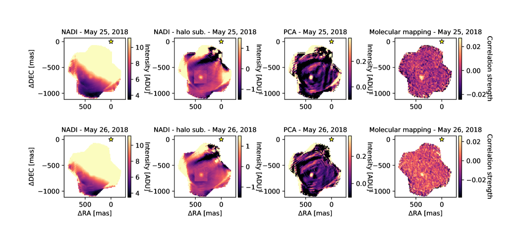
Figure 1: Detection of HIP 65426 b with SINFONI using (from left to right) a simple derotation and stack of the individual cubes (nADI), a removal of the halo at each wavelength using a circular profile and a local fit with a 2D polynomials, the PCA algorithm (3 modes), and the molecular mapping with an Exo-REM model at $\mathrm{T_{eff}}$=1600 K, log(g)=4.0 dex, [M/H]=0 dex, C/O=0.35 (at 20   km s^-1).

Adaptive-optics-fed integral-field spectrographs (IFS) operating at medium spectral resolving power ($R_{\lambda}=2000-5000$) in the near-infrared such as SINFONI at VLT, NIFS at Gemini-North, or OSIRIS at Keck offer to partly deblend a rich set of molecular absorption contained in the exoplanet spectra. They have been used for gathering the spectra of young low-mass companions at large distance from their host stars ($>$1”) or in systems with moderate contrasts in the near infrared (McElwain et al., 2007; Seifahrt et al., 2007; Schmidt et al., 2008; Lavigne et al., 2009; Bowler et al., 2011; Bonnefoy et al., 2014; Schmidt et al., 2014; Bowler & Hillenbrand, 2015; Bowler et al., 2017; Daemgen et al., 2017). More recently, high-contrast imaging techniques such as the Angular-Differential-Imaging (e.g. ADI, Marois et al., 2006) have been implemented on these instruments and allowed for characterizing companions at shorter separations ($\rho<$1”; Bowler et al., 2010; Meshkat et al., 2015; Hoeijmakers et al., 2018; Mesa et al., 2019; Christiaens et al., 2019). Using OSIRIS, Konopacky et al. (2013) and Barman et al. (2015) detected carbon monoxide and water in the spectrum of HR 8799 b and c which they confirmed using the cross-correlation of the spectra with templates of pure H₂O, CO, and CH₄ absorption. The cross-correlation approach has been generalized to all spaxel contained in IFS datacubes by Hoeijmakers et al. (2018) following a modified prescription of the algorithm described in Sparks & Ford (2002). This “molecular mapping” method allows for getting rid of the remaining stellar flux residuals including the quasi-static noise created by the IFS optical elements (Janson et al., 2008) while providing an interesting mean to identify unambiguously cool companions and characterize their properties ($\mathrm{T_{eff}}$, log(g), [M/H], composition, and radial velocity). The approach has thus far been used on a limited set of data ($\beta$ Pictoris b, HR8799 b; Hoeijmakers et al., 2018; Petit dit de la Roche et al., 2018), and its performances and limitations are yet to be investigated on additional data and against alternative methods exploiting the IFS data diversity (e.g., Marois et al., 2006; Thatte et al., 2007; Ruffio et al., 2019).

HIP 65426 b (Chauvin et al., 2017) is the first exoplanet discovered with the VLT/SPHERE instrument, at a projected separation of 92 au from the young ($14\pm 4$ Myr) intermediate-mass star HIP 65426 (A2V, M=1.96$\pm$0.04 M_⊙). The star is located at a distance of $111.4\pm 3.8$ pc (Gaia Collaboration et al., 2016), and belongs to the Lower Centautus-Crux (hereafter LCC) association (de Zeeuw et al., 1999; Rizzuto et al., 2011). The low-resolution Y to H-band photometry and spectra of HIP 65426 b indicate the object has a L$6\pm 1$ spectral type with clear signatures of reduced surface gravity (Chauvin et al., 2017). The hot-start evolutionary models (Baraffe et al., 2003; Chabrier et al., 2000; Mordasini, 2013) predict $M_{b}\,=\,6\,-\,12$ $\mathrm{M_{Jup}}$  in the planetary-mass range. Atmospheric models estimate $\mathrm{T_{eff}}$ in the range $1100-1700$ K, a surface gravity log(g) lower than 5 dex, and a radius from 1 to 1.8 $\mathrm{R_{Jup}}$. These physical properties were confirmed by Cheetham et al. (2019) who analysed the SPHERE data together with new VLT/NaCo L and M bands (3.49-4.11 $\mathrm{\mu m}$  and 4.48-5.07 $\mathrm{\mu m}$) observations. They found $\mathrm{T_{eff}}\,=\,1618\pm 7$ K, $log(g)\,=\,3.78_{-0.03}^{+0.04}$ dex and $R\,=\,1.17\pm 0.04$ $\mathrm{R_{Jup}}$  and estimate a new mass $M\,=\,8\pm 1$ $\mathrm{M_{Jup}}$ (statistical errors). The relatively low mass ratio of HIP 65426 b with A ($M_{b}/M_{A}\sim$0.004), its intermediate semi-major axis ($110^{+90}_{-30}$ au, Cheetham et al., 2019), and the non-detection of a debris disk in the system (Chauvin et al., 2017) question the origin of HIP 65426 b and makes the system an interesting testbed for planet formation theories. Marleau et al. (2019a) explored formation scenarios for HIP 65426 b, including the evolution of the protoplanetary disc and the gravitational interaction with possible further companions in the system.

In this paper, we analyse medium-resolution ($R_{\lambda}\sim$5500) K-band data of HIP 65426 b collected with the VLT/SINFONI IFS to characterize the exoplanet and evaluate the potential of the molecular mapping technique. We describe in Section 1 the observations and data reduction based on the molecular mapping and classical ADI extraction techniques. We characterize the planet in Section 3 using the new spectroscopic data, and discuss our results in the Section 4.

2 Observations and data reduction

2.1 Observations

HIP 65426 was observed on May 25 and May 26, 2018 with the VLT/SINFONI instrument (program 0101.C-0840; PI Hoeijmakers) mounted at the Cassegrain focus of VLT/UT4 (see Table 1). SINFONI is made of a custom adaptive optics module (MACAO) and of an IFS (SPIFFI). SPIFFI cuts the field-of-view into 32 horizontal slices (slitlets), which are re-aligned to form a pseudo-slit, and dispersed by a grating on a Hawaii 2RG (2k$\times$2k) detector (Eisenhauer et al., 2003; Bonnet et al., 2004).

The instrument was operated with pre-optics and a grating sampling a 0.8”$\times$0.8” field of view with rectangular spaxels of 12.5$\times$25 mas size, from 1.928-2.471 $\mathrm{\mu m}$, at a spectral resolution $R_{\lambda}=\lambda/\Delta\lambda\sim$ 5220 (from the width of the line-spread function). MACAO was used at all time during the observations with the primary star as a reference for the wave-front sensing. The de-rotator at the telescope focus was in addition turned off to allow for pupil-tracking observations.

At each night, the star was first placed inside the field-of-view and two 10 s integrations were obtained. The core of the star point-spread-function (PSF) was then moved outside of the field of view with the instrument field selector and a sequence of 100 s integrations centered on the expected position of the planet were performed. This strategy is similar to the one adopted on $\beta$ Pictoris (Hoeijmakers et al., 2018, Bonnefoy et al. in prep). It reduces the impact of the read-out in the noise budget while avoiding any persistence on the detector of SPIFFI.

2.2 Cube building and registration

The data were initially reduced with the SINFONI data handling pipeline v3.2.3 (Abuter et al., 2006) through the EsoReflex environment (Freudling et al., 2013). The pipeline used a set of calibration frames obtained at day time to perform basic cosmetic steps on the raw bi-dimensional science frames and correct them from the distortion. The pipeline also identified the position of slitlets on the frames and the wavelength associated to each pixel before building a serie of datacubes corresponding to each exposure. The sky emission was evaluated and removed through the field of view using the methods from Davies (2007).

We used on top of the ESO recipes the Toolkit for Exoplanet deTection and chaRacterization with IfS (hereafter TExTRIS) to optimize our cubes for the high-contrast science (The main steps are described below, see Bonnefoy et al. in prep for another application of this tool). The toolkit first corrected the raw SINFONI data from various noises occurring on the detector described in Bonnefoy et al. (2014).

TExTRIS also mitigated two different effects affecting the cubes:

• we corrected an incorrect estimate of the slitlet positions on the raw science frame and masked the first two and last two columns of spaxels in the cubes which are affected by cross-talk at the slitlet edges. This step is critical for removing important stellar flux residual at the edges of the field of view and getting an accurate knowledge of the star position outside the field of view.

• we re-examined the wavelength calibration performed by the ESO pipeline by comparing the many telluric absorption lines contained in each spaxel to a model generated for the observing conditions with the python module skycalc_ipy and based on the ESO Skycalc tool (Noll, S. et al., 2012; Jones, A. et al., 2013). The method was shown to be critical for yielding a robust radial velocity measurement of $\beta$ Pictoris b (Bonnefoy et al, in prep) and improving the capabilities of the molecular mapping technique (see Section 2.4). It is applicable whenever the spaxels contain enough stellar light to evidence the telluric absorptions. The shifts were evaluated on each input cube across the field of view. A master median-combined map of velocity shift was then created and each individual cube was corrected from the effect. We find spaxels are red-shifted by 21.6 and 16.4   km s^-1  on average (0.6 and 4.2   km s^-1  dispersion along the sequences) on the first and second night of observations, respectively. We found and corrected additional relative $\sim$   km s^-1  shifts from spaxel to spaxel across the field. These smaller shifts are visible at the same position for all cubes along the sequence and point toward differential errors on the wavelength solutions between the slitlets. We validated this re-calibration on the final products in the Appendix A using an independent method relying on OH sky emission lines.

We used TExTRIS to re-compute the parallactic angles and rotator angular offsets following the method we described in Meshkat et al. (2015) to allow for realigning the cubes to the North.

To conclude, the software retrieved the position of the star outside the field of view. SINFONI lacks an atmospheric dispersion corrector, which makes the registration more complex. We followed a three-step strategy:

• the position of the star was first evaluated at each wavelength in the last cube corresponding to the 10 s exposure using a Moffat function. The drift was fitted with a low-order polynomial;

• we accounted for the field selector offsets, the field rotation, and the change in atmospheric refraction to measure the star position outside the field of view in the first 100 s exposure. The theoretical change of the star position due to atmospheric refraction was computed using empirical formulas reported into the source code of the SINFONI data handling pipeline recipes and adapted to the case of the pupil-tracking mode (see the pipeline user manual);

• we iterated over the next 100 s exposures using our computed change of theoretical atmospheric refraction and the evolution of the parallactic angle.

We assumed for that purpose a pivot point located at the center of the field of view (X=32, Y=32; see the ESO manual). The accuracy on the position of that pivot point is however tied to the proper correction of the slitlet edges which we evaluate to be accurate to $\sim$1 pixel. We therefore explored different pivot point locations within a 3 pixel-wide box centered on the theoretical ones, with 0.5 pixel increments and concluded that the theoretical value was offering the strongest cross-correlation signal (see section 3) on the planet on both night in our data. The strategy was vetted on similar data obtained on $\beta$ Pictoris b (Bonnefoy et al., in prep), and provides a centering with an accuracy better than a spaxel ($\sim$12.5 mas) along the sequence.

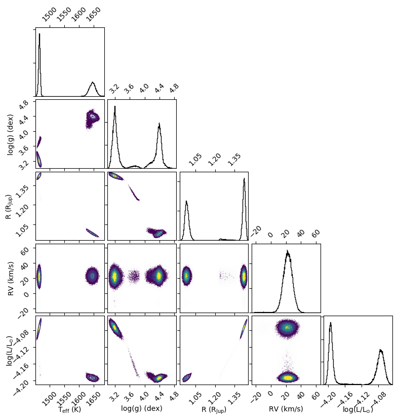
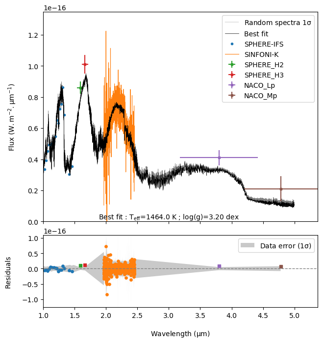
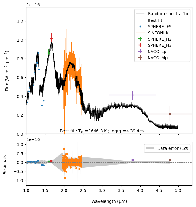
Figure 2: Top : Bi-modal posterior distribution inferred from ForMoSA using the BT-SETTL15 models. Bottom left and right : comparison between the best fit and the observed data for the low $\mathrm{T_{eff}}$  and the high $\mathrm{T_{eff}}$  modes, respectively. The data points were obtained using the low-resolution SPHERE-IFS spectrum (R$\simeq$30-50; blue points, Chauvin et al., 2017), the SPHERE-IRDIS H-band photometry (green and red points; Cheetham et al., 2019), our medium-resolution SINFONI spectrum (R$\simeq$5500); orange points, this work), and the NaCo L’ and M’-band photometry (purple and brown points, respectively; Cheetham et al., 2019). We overlaid 50 synthetic spectra picked randomly within the 1-$\sigma$ envelop of each posterior in grey.

2.3 Extraction of emission spectra using the ADI

We applied the angular differential imaging technique (Marois et al., 2006) on each cube slice to evaluate and remove the halo. Both the classic-ADI approach and the PCA (5 modes) allow to retrieve the planet at each epoch with a shape and size compatible with the PSF (Figure 1). This validates further the star registration process. The post-ADI cubes are affected by residuals from the diffraction pattern created by the telescope spiders (the negative and positive lines near the edges of the field of view). The PCA appears to mitigate some of those residuals. We also used the nADI approach considering a simple re-alignment of the individual cubes to the North and a stack. The nADI reveals the planet on top of the stellar halo. We found the halo could be subtracted on data from May 25, 2018 with the nADI approach removing a circular profile at first and fitting the residuals in a 20 pixel square box around the planet with a 2D polynomial. The box size was chosen to avoid introducing artefacts at the edges of the field of view that could bias the fit while allowing for having a stable (converged) fit of the halo at each wavelength (Appendix B). This method fails to provide an accurate removal of the halo in the data from May 26, 2018 obtained in poorer conditions. The companion spectrum was extracted within a 75 mas circular aperture in the PCA and the halo-subtracted nADI cubes. We used the average flux of the residuals in the halo-substracted nADI cubes in an annuli of radius 50-113mas to estimate the error bars on the planet flux. A spectrum of the star was obtained from the short-exposures datacubes (see Table 1) within the same aperture and allowed to compute the flux ratio with the planet at each wavelengths. This ratio was multiplied by a BT-NEXTGEN synthetic spectrum (Allard et al., 2012) at $\mathrm{T_{eff}}$=8400K, log g = 3.5 dex, and M/H=0 dex degraded to the resolution of SINFONI and flux-calibrated on the TYCHO (B, V), 2MASS (J, H, K), DENIS (K), WISE (W1 to W4) and AKARI (S9W) photometry (Høg et al., 2000; Cutri et al., 2003; DENIS Consortium, 2005; Cutri & et al., 2012) of the star extracted from the VOSA (Bayo et al., 2008) SED analyser. This allowed us to obtain final telluric-free spectra of the planet. The spectra of HIP 65426 b extracted from the PCA on both nights have an identical shape but are noisier than the spectrum extracted from the nADI-processed datacubes obtained at one epoch (see Appendix B). The later spectrum absolute flux is in excellent agreement with the K1 and K2 photometry reported in Cheetham et al. (2019). We chose to use it for the analysis presented in Section 3.

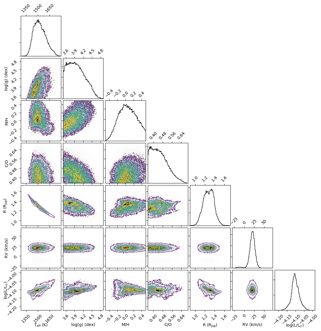
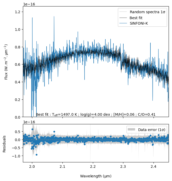
Figure 3: Same as Figure 2 but with the grid of Exo-REM spectra and applicable to the K-band SINFONI data.

2.4 Molecular mapping

We implemented in TExTRIS the ”molecular mapping” technique following the main steps described in Hoeijmakers et al. (2018). A reference spectrum of the star was first extracted in each cube from the median-combination of the 1% most illuminated spaxels in the field-of-view. This reference spectrum contains a representative set of telluric and stellar features (here Brackett $\gamma$), but does not model the changing slope of the spectra of each individual spaxel across the field-of-view because of the evolution of the SINFONI PSF with wavelength. A model of the stellar emission was then created for each spaxel (i,j) computing the ratio between the spaxel (i,j) and the referenced spectrum. The ratio was smoothed with a Gaussian boxcar of width 22 Å (10 spectral elements) and used for computing a slope-corrected model of each spaxel (i,j). The model was then subtracted to the spaxels to create a cube of residuals where both the continuum emission of the star and of any companion is removed. This step was repeated onto each datacube for the sequence once.

We then cross-correlated each spaxel with a template spectrum (see Section 3.1) smoothed to the spectral resolution of SINFONI and for which the continuum had been removed beforehand using a gaussian boxcare of 20Å  too. The cross-correlation function (CCF) was performed with the Python module crosscorrRV from the PyAstronomy package customized to include a normalization of the CCF following Briechle & Hanebeck (2001). The CCF explores velocities from -100 to +100   km s^-1  in steps of 8  km s^-1 ($\sim$4 times the original sampling of the data in velocity). The individual cubes of cross-correlation function were then corrected from the barycentric velocity using the Python module barycorrpy (Kanodia & Wright, 2018b, a) and combined once phased in velocity. The planet is re-detected at a separation $\rho=812\pm 18$ mas and PA$=150.2\pm 1.2^{\circ}$, and $\rho=796\pm 18$ mas and PA$=150.6\pm 1.2^{\circ}$ on May 25^th and 26^th, 2018, respectively (the error bars correspond to 1 pixel in the SINFONI field). The SINFONI astrometry is compatible within $2\sigma$ with the one measured on VLT/SPHERE data from May 12^th, 2018 ($\rho=822.9\pm 2.0$mas, PA$=149.85\pm 0.15^{\circ}$) by Cheetham et al. (2019) while it does not rely on a proper calibration of the spaxel size and absolute orientation of the instrument. We present an analysis of the correlation signals in Section 3.3.

3 Physical properties

We adopted two independent methods for deriving the physical properties of HIP 65426 b’s atmosphere. We used a classical forward modelling approach that compares observed spectra with grids of pre-computed synthetic spectra using Bayesian inference methods to estimate posteriors on a set of parameters. We also applied the molecular mapping technique studying the evolution of the cross-correlation signal at the planet location for different molecular templates or grids of atmospheric models used as input. For both methods, we considered grids of BT-SETTL15 and Exo-REM  (Allard et al., 2012; Charnay et al., 2018) synthetic spectra. The corresponding models are described below.

3.1 Atmospheric models

3.1.1 BT-SETTL15

BT-SETTL15 includes a 1D cloud model where the abundance and size distribution of 55 types of grain are determined comparing the timescale of the condensation, the coalescence, the gravitational settling and the mixing of these solids supposed spherical. The details of each solids and chemical elements included in the model are described in Rajpurohit et al. (2018). The opacities in the spectral energy distribution (hereafter SED) are calculated line by line and the overall radiative transfer is carried on by the PHOENIX code (Hauschildt et al., 1997; Allard et al., 2001). The convection is handled following the mixing-length theory, and works at hydrostatic and chemical equilibrium. The model also accounts for non-equilibrium chemistry between CO, CH₄, CO₂, N₂, and NH₃. The grid we used (CIFIST2011c) considers a $\mathrm{T_{eff}}$ from 300 to 7000 K in steps of 100 K, a surface gravity (hereafter log(g)) from 2.5 to 5.5 dex in steps of 0.5 dex. For computing efficiency, we used models with $\mathrm{T_{eff}}$ in the range of 1200-2000 K which is a conservative prior considering the previous spectral characterization of HIP 65426 b. The grid does not allow for an exploration of non-solar metallicities in that temperature range.

3.1.2 Exo-REM

Exo-REM is an atmospheric radiative-convective equilibrium model including in addition a cloud description well suited for reproducing the spectra of brown dwarfs and exoplanets where dust dominates, especially at the L-T transition. Much like the BT-SETTL15  models, the atmosphere is cut into 64 pressure levels. The flux over these layers is calculated iteratively using a constrained linear inversion method, for a radiative-convective equilibrium. The initial abundances of each chemical element are first established using the values tabulated in Lodders (2010). The model includes the collision-induced absorptions of H₂–H₂ and H₂–He, ro-vibrational bands from nine molecules (H₂O, CH₄, CO, CO₂, NH₃, PH₃, TiO, VO, and FeH), and resonant lines from Na and K. As BT-SETTL15, Exo-REM accounts for non-equilibrium chemistry between CO, CH₄, CO₂, and NH₃ due to vertical mixing. The abundances of the other species are computed at thermochemical equilibrium. The vertical mixing is parametrized by an eddy mixing coefficient from cloud-free simulations. The cloud model includes the formation of iron, silicate, Na₂S, KCl, and water clouds. This grid was generated exclusively for this study and provides spectra from 1.887 $\mathrm{\mu m}$  to 2.500 $\mathrm{\mu m}$  and includes four free parameters: The $\mathrm{T_{eff}}$  from 300 to 1800 K in steps of 50 K, the log(g) from 3.5 to 5.0 dex in steps of 0.5 dex, the [M/H] for -0.5 to 0.5 in steps of 0.5 dex and the [C/O] from 0.35 to 0.8, in steps of 0.05. We notice that synthetic spectra are available at higher $\mathrm{T_{eff}}$ but we have chosen to not include them due to the non convergence of these models beyond $\mathrm{T_{eff}}$=1800 K.

3.2 Bayesian inference of the spectro-photometry

Table 2: Estimation of the atmospheric parameters of HIP 65426 b for each grid of synthetic pre-computed spectra and for each method. The errors are statistical and result from the Bayesian inversion. In the case of posteriors located at the edge of the grid, an upper/lower limit is defined for the corresponding parameter.

BT-SETTL15
	$\mathrm{T_{eff}}$	log(g)	R	RV	$\mathrm{log(L/L_{\odot})}$
	(K)	(dex)	($\mathrm{R_{Jup}}$)	( km s-1)
ForMoSA
1.0 - 4.7 $\mathrm{\mu m}$ Low $\mathrm{T_{eff}}$ with continuum	1464${}_{-3}^{+3}$	3.20${}_{-0.06}^{+0.09}$	1.42${}_{-0.01}^{+0.01}$	21.8${}_{-6.2}^{+6.3}$	-4.07${}_{-0.01}^{+0.01}$
1.0 - 4.7 $\mathrm{\mu m}$ High $\mathrm{T_{eff}}$ with continuum	1645${}_{-11}^{+10}$	4.38${}_{-0.11}^{+0.07}$	0.98${}_{-0.01}^{+0.02}$	22.8${}_{-5.6}^{+5.5}$	-4.19${}_{-0.01}^{+0.01}$
K band Low $\mathrm{T_{eff}}$ with continuum	1461${}_{-6}^{+6}$	$\leq$ 3.25	1.43${}_{-0.02}^{+0.02}$	21.7${}_{-6.2}^{+6.1}$	-4.09${}_{-0.02}^{+0.02}$
K band High $\mathrm{T_{eff}}$  with continuum	1610${}_{-37}^{+20}$	4.19${}_{-0.13}^{+0.14}$	1.03${}_{-0.04}^{+0.05}$	22.3${}_{-6.1}^{+6.0}$	-4.19${}_{-0.01}^{+0.01}$
K band without the continuum	1633${}_{-260}^{+234}$	$\leq$ 4.00	-	18.7${}_{-16.8}^{+14.0}$	-
TExTRIS
K band Low $\mathrm{T_{eff}}$ without the continuum	1400	3.0	-	20${}_{-8}^{+8}$	-
K band High $\mathrm{T_{eff}}$ without the continuum	1700	3.5	-	20${}_{-8}^{+8}$	-
$\chi^{2}$ minimization
K band Low $\mathrm{T_{eff}}$ without the continuum	1400	3.5	-	-	-
K band High $\mathrm{T_{eff}}$ without the continuum	1800	3.5	-	-	-

Exo-REM
	$\mathrm{T_{eff}}$	log(g)	[M/H]	C/O	R	RV	$\mathrm{log(L/L_{\odot})}$
	(K)	(dex)			($\mathrm{R_{Jup}}$)	( km s-1)
ForMoSA
K band with continuum	1518${}_{-71}^{+88}$	$\leq$ 4.20	0.05${}_{-0.22}^{+0.24}$	$\leq$ 0.50	1.28${}_{-0.11}^{+0.10}$	20.2${}_{-6.4}^{+6.0}$	-4.10${}_{-0.2}^{+0.2}$
K band without the continuum	1639${}_{-187}^{+141}$	$\leq$ 4.5	0.02${}_{-0.35}^{+0.35}$	$\leq$ 0.55	-	17.0${}_{-15.0}^{+10.8}$	-
TExTRIS
K band without the continuum	1700	3.5	0.0	0.40	-	20${}_{-8}^{+8}$	-
$\chi^{2}$ minimization
K band without the continuum	1500	3.5	0.0	0.40	-	-	-

We used the ForMoSA code presented in Petrus et al. (2020) to compare the synthetic spectra to the data following the forward-modelling approach. ForMoSA relies on the Nested Sampling algorithm (Skilling, 2006) to determine the posterior distribution function of a set of free parameters in the models. This method performs a global exploration of the model parameter space to look for local maxima of likelihoods following an iterative method which isolates progressively restrained area of iso-likelihood while converging toward the maximum values. That avoids missing local maxima of likelihood and allows to evaluate the Bayesian evidence that can be used for performing model selection (Trotta, 2008).

Because the Bayesian inference implies to generate random points with continuous distribution inside the parameter space, we chose to reduce the step of each model grids by interpolating them with the N-dimensional linear interpolation python package griddata which is triangulating the input data with Qhull before applying barycentric interpolation. The interpolated steps of the BT-SETTL15 grids are 10 K for the $\mathrm{T_{eff}}$  and 0.1 dex for the log(g) while the interpolated steps of the Exo-REM grids are 10 K for the $\mathrm{T_{eff}}$, 0.1 dex for the log(g), 0.1 for the metallicity and 0.05 for the C/O ratio. It increases the accuracy of the second interpolation step which occurs over the course of the nested sampling process when a new random point is generated in the parameter space. That interpolation is based on N-dimensional weighted mean of the closest neighboring spectra inside the interpolated grid. The physical parameters derived by ForMoSA are summarized in Table 2. We stress that the errors given by ForMoSA are statistical and have been determined for each parameter as the range which encompasses 68% of the solutions in each posterior, they do not include possible systematical errors in models that are difficult to quantify (see Petrus et al. 2020). Whenever the posterior distribution do not show a maximum (e.g. C/O ratio), we defined an upper limit on the given parameter encompassing 68% of the posterior distribution starting from the posterior maximum. Extended grids would be needed to constrain these parameters, but such analysis is left for future work. The best fits to the data, obtained by using 20 000 living points in the nested sampling algorithm, are presented in Figures 2 and 3 for both families of atmospheric models.

When the 1.0-4.7 $\mathrm{\mu m}$ spectral energy distribution is compared to the BT-SETTL15 models (Figure 2), two distinct groups of solutions emerge: at “low-$\mathrm{T_{eff}}$” ($\mathrm{T_{eff}}$=1464$\pm$3 K) and at “high-$\mathrm{T_{eff}}$” ($\mathrm{T_{eff}}$=1645$\pm$10 K). Both sets of solutions were explored within separate runs using flat priors between 1200-1500 K and 1500-2000 K, respectively. The results are shown in Table 2 together with the data and the distribution of 50 synthetic spectra corresponding to draws within the 1-$\sigma$ interval of each posterior. The residuals between the observations and the best solutions are also shown, and compared with the data error bars (grey area).

The L’ and M’ photometry is up to 1.5$\sigma$ above the predictions. This may be due to the lack of exploration of non-solar atmospheric composition by the BT-SETTL models, to an imperfect handling of the non-equilibrium chemistry which tend to enhance the L’ and M’ band fluxes in young L-T transition objects (Hubeny & Burrows, 2007; Skemer et al., 2014; Moses et al., 2016; Stone et al., 2016) or cloud properties (e.g., Skemer et al., 2014), or even to excess emission from a putative circumstellar disk (Christiaens et al., 2019). Similar deviations beyond 2.5 $\mu$m are also seen in the spectral-energy-distribution fit of mid and late-L type brown dwarfs from Upper-Scorpius (Lodieu et al., 2018) using the same models. We also note that the H-band fluxes (SPHERE) are not reproduced well in the case of the ”low-$\mathrm{T_{eff}}$” solution while the L’ and M’ band fluxes and the water-band absorption from 1.35 to 1.45 $\mu$m are better represented. Previous version of the BT-SETTL models already failed representing the shape of the H band of young L-dwarfs sampled by the SPHERE H-band filters (Manjavacas et al., 2014). Removing these points do not remove the bi-modal posterior distribution.

Conversely, one unique set of solutions at intermediate $\mathrm{T_{eff}}$ is found with the Exo-REM models (Figure 3) which allow for an exploration of non-solar abundances. Conversely, both models tend to predict close mono-modal solutions when the continuum is removed that are in better agreement with the ones found by Cheetham et al. (2019) made without the SINFONI data albeit with much larger uncertainties.

A consistent radial velocity of 22$\pm$6   km s^-1ãnd 20$\pm$6   km s^-1 is found for HIP 65426 b using the BT-SETTL15 and Exo-REM models at K-band, respectively.

We used the $\mathrm{T_{eff}}$ infered from ForMoSA and the DUSTY evolutionary model (Chabrier et al., 2000) to derive a planet mass between 8.1 and 10.0 $\mathrm{M_{Jup}}$  consistent with the values from Marleau et al. (2019b), and a radius between 1.48 and 1.53 RJup  . The radii obtained with ForMoSA and the BT-SETTL models for the ”cold-$\mathrm{T_{eff}}$”   solution are in better agreement with the tracks while those obtained for the ”high-$\mathrm{T_{eff}}$¨ prediction are clearly at odd with the expected evolution of a young Jupiter such as HIP 65426b. The Exo-REM models also tend to under-predict the radii, but at reduced scale. These differences are well documented already for young L-type planets such as HIP 65426b (e.g., Marley et al., 2012; De Rosa et al., 2016) and could be explained by the imperfect description of the cloud physics and opacity.

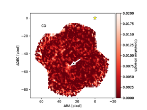
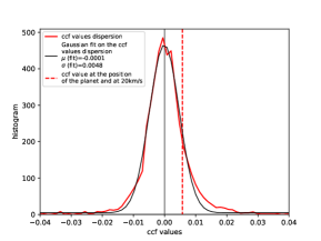
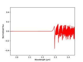
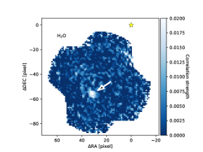
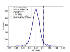
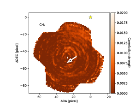
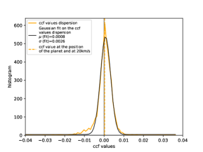
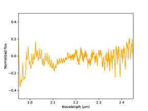
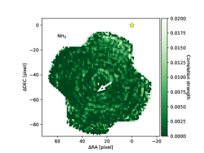
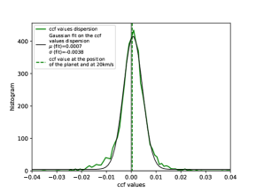
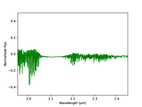
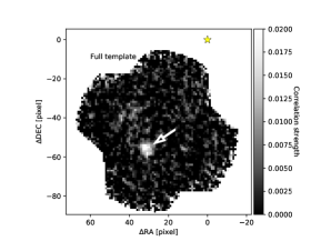
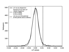
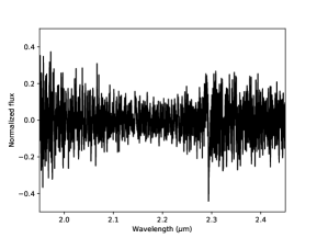
Figure 4: Left : Maps of cross-correlation between SINFONI data of HIP 65426 b and templates of molecules ¹²CO, H₂O, CH₄, NH₃ and full molecule template (top to bottom respectively) at a velocity of 20   km s^-1. The star represents the position of the host star which is out of field. We detect the companion with the full molecule template (SNR=2.5), H₂O (SNR=2.2) and possibly with the ¹²CO (SNR=1.1). Center : Distributions of cross-correlation values in the integrated cross-correlation cube for each position. The correlation signal is significant for the full molecule template, H₂O and ¹²CO but not for CH₄ and NH₃. Right: molecular template.

3.3 Characterization with the molecular mapping

3.3.1 Extraction of the planet’s correlation signal

We ran the molecular mapping steps with the TExTRIS package (Section 2.4) on the molecular templates (see Section 3.3.2) and the grids of Exo-REM and BT-SETTL15 model spectra (see Section 3.3.3). The tool was parallelized to gain computation time and produced as many cross-correlation maps as input model spectra. The planet is detected with a radial velocity of 20$\pm$8  km s^-1  (see Figures 1). We extracted the cross-correlation signal in the correlation maps by averaging the cross-correlation function over the FWHM of the auto-correlation, centered on the planet radial velocity to produce averaged correlation maps and within a circular aperture centered on the planet position of 4 pixels radius ($\sim$FWHM of the PSF) to extract the correlation signal of the planet. We detail below our exploitation of the correlation signal to characterize the properties of the planet.

3.3.2 Molecular template analysis

We used pre-computed templates of individual molecules (¹³CO, ¹²CO, CO₂, CH₄, FeH, H₂O, HDO, K, NH₃, Na, PH₃, TiO and VO) as input of TExTRIS to evaluate whether these species produce a strong set of absorption in the planet spectrum. The templates were computed with the Exo-REM model assuming the pressure-temperature profile of a solar-metallicity atmosphere with $\mathrm{T_{eff}}$=1700 K, log(g)=4.0 dex (e.g, a generic model close to the physical properties of HIP 65426 b). We show in Figure 4 (left column) the averaged correlation maps for the CO, H₂O, CH₄ and NH₃ templates, and with the full molecule template ($\mathrm{T_{eff}}$=1700 K, log(g)=4.0 dex, [M/H]=0.0, C/O=0.50). The planet is detected with the full molecule template, the H₂O template and marginally with the ¹²CO template. The distribution of correlation signals (see Figure 4, right column) shows a Gaussian distribution and indicates a detection at a signal-to-noise of 2.5, 2.2 and 1.2 for the full molecule template, the H₂O and ¹²CO templates, respectively. This is consistent with the mid-L spectral type of the object.

The lack of a clear detection of the ¹²CO is unexpected for a L6 object and is discussed in the Section 4.1.1.

3.3.3 Grids of synthetic spectra exploration

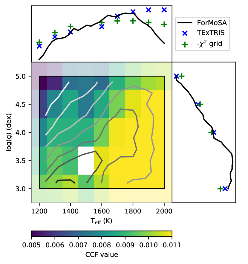
Figure 5: Comparison between the correlation signal of each spectrum of the grid BT-SETTL15 obtained with TExTRIS (color map) and the 2D-posterior obtained with ForMoSA (grey contours). We also compare the normalized 1D-posterior obtained with ForMoSA on the K band without the continuum (black line) with the normalized 1D-pseudo-posteriors extracted from the correlation signal map (blue cross) and a $\chi^{2}$ map (green cross) for the $\mathrm{T_{eff}}$  and the log(g) (top and right panel respectively). The white rectangle corresponds to an non-converged synthetic spectra.

As a following step, we explored the evolution of the cross-correlation signal over the synthetic grid of spectra from the BT-SETTL15 and Exo-REM models. Synthetic spectra with anomalous spectral slopes indicative of non-converged cloud models were excluded and are reported as white rectangles. The application with the BT-SETTL15 grid is shown in Figure 5 giving the correlation signal evolution with the effective temperature and the surface gravity. The 2D posterior distribution obtained with the ForMoSA code on the continuum-removed SINFONI spectrum (see Section 3.2) is overlaid. We also show the corresponding 1D posteriors along with the averaged $\chi^{2}$ and mean correlation signals (“pseudo-1D-posteriors”). The $\chi^{2}$ pseudo-1D-posteriors starts from the original grid of models. We note that this alternative approach to the forward modeling one also identifies two distinct modes of physical parameters for HIP 65426 b at “low-$\mathrm{T_{eff}}$” ($\mathrm{T_{eff}}$$\simeq$1400 K) and “high-$\mathrm{T_{eff}}$” ($\mathrm{T_{eff}}$$\simeq$1800 K).

A similar analysis with the Exo-REM model grid are shown in Figure 6 considering different layouts in the parameter space explored. Their exploitation also shows a similar behavior than previously and favors one family of solutions with $\mathrm{T_{eff}}$=1700 K, log(g)=3.5, [M/H]=0.0 and C/O=0.40. For both models, the detailed set of physical parameters maximizing the correlation signal are reported in Table 2 for the BT-SETTL15 and Exo-REM models. We notice that the maximum of the CCF value obtained with both model are similar ($\sim$ 0.011). The CCF signal using the Exo-REM models is maximized at solar-metallicity, which correspond ”de-facto” to the one of the BT-SETTL15 models.

The comparison of both approaches (forward modeling versus molecular mapping) for the characterization of planetary signals is discussed below, together with the physical properties and possible origin of HIP 65426 b.

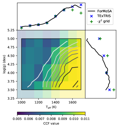
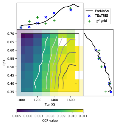
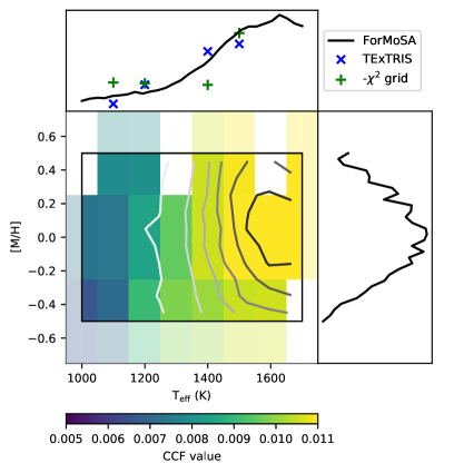
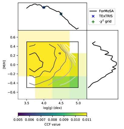
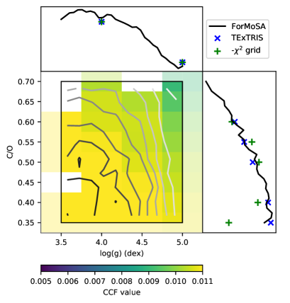
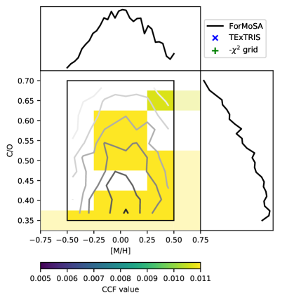
Figure 6: Same as in the Figure 5 but with the grid Exo-REM. We considered different layouts around the set of parameters that maximise the CCF in each direction of the parameter space. Models at $\mathrm{T_{eff}}$=1800K are unconverged at the given [M/H] and/or C/O, and/or log (g) so that the corresponding CCF values and posteriors stop at $\mathrm{T_{eff}}$=1700K.

4 Discussion

4.1 Performances and limitations of our data analysis

4.1.1 The molecular mapping on noisy data

The exposure time calculator (ETC- of SINFONI estimates a theoretical maximum S/N=15.2 from 2.1 to 2.15 $\mu$m for the first night of observations. We measure a S/N of 9.7 on the extracted spectrum over a similar wavelength interval (see Appendix B). The difference may be due to wavelength-to-wavelength noise introduced by the extraction process. The data are read-out noise limited because of the small integration time used for avoiding the persistence on the detector. This advocates for the use of specific high-contrast modes on such medium-resolution IFUs (e.g., GTC/FRIDA, ELT/HARMONI; N’Diaye et al., 2018; Carlotti et al., 2018).

The observations of HIP 65426 b offer an interesting test-case of the molecular mapping method when applied in the low S/N regime. In such a case, only the strongest molecular absorptions will contribute to the correlation signal. The H₂O tend to produce a larger amount of strong lines compared to ¹²CO. The ¹²CO lines are spread in a narrow range of wavelength where the theoretical S/N predicted by the ETC is lower (10.5 for wavelengths longward of 2.29 $\mu$m) due to the numerous telluric lines and the lower transmission of the K-band filter of the instrument. Conversely, the set of narrow water absorption are found as a set of partly blended features at the resolution of SINFONI and spread over the entire K-band (Figure 4). This explains why the ¹²CO does not produce a strong correlation signal as would naively be expected for a mid-L type exoplanet. We investigated the detection capability of the molecular mapping using the CO template further in the Appendix C injecting fake planets at different C/O ratio into our datacube. The tests reveal the ability of the method for recovering a planet with a noiseless spectral signature close to the one of HIP 65426b at a low S/N. We show in addition that the significance of the detection drops for synthetic planets with low C/O ratio for which the strongest CO overtone is shallower.

We show in Figure 7 the correlation signal between the extracted SINFONI spectrum of the planet (continuum-subtracted) and the molecular templates. We confirm the conclusions from Figure 4 and in particular the faintness of the correlation signal of ¹²CO with respect to H₂O. To conclude, the figure also reveals additional correlation and anti-correlation peaks over the velocity span. As noted by Hoeijmakers et al. (2018), some of these peaks are likely to be caused by the regular spacing of molecular absorption both in the template and exoplanet spectra (overtones). This was checked by computing the auto-correlation of the templates and justifies the use of the spatial distribution of CCF values for computing a signal-to-noise rather than the velocity dimension. The overtones appear at different velocities in the various molecules and therefore the correlation of full synthetic spectra combining all the molecular absorption offer to reduce these parasitic signals with respect to the main correlation peak in the velocity space.

These features are slightly reduced and the central correlation peak is enhanced when using a full synthetic spectrum corresponding to the $\mathrm{T_{eff}}$  log g, and composition assumed for the templates of individual molecules. For all these reasons, the use of full synthetic spectra with respect to templates of individual molecules offers a more robust way of characterizing any object and achieving a convincing detection of new ones.

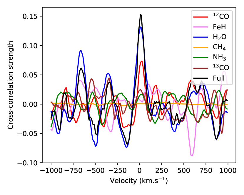
Figure 7: Cross-correlation signals obtained when using the continuum-subtracted spectrum of HIP 65426 b and the molecular templates (color) or a full Exo-REM spectrum at $\mathrm{T_{eff}}$=1700K, log g=4.0 and solar abundances (black).

4.1.2 Comparison of the characterization approaches

In this study, we compare three different approaches to determine the physical parameters of HIP 65426 b: a standard $\chi^{2}$ minimization, a Bayesian inference with the code ForMoSA, and the molecular mapping with the code TExTRIS. We show in the Figures 5 and 6, and Table 2 that all three methods yield consistent results.

The coherency between the $\chi^{2}$ minimization and the Bayesian inference stems from our assumption of Gaussian distribution of uncertainties on the observed spectra and the lack of correlations between the data-points. The likelihood and the cross-correlation function are related assuming the same underlying hypothesis on the data (Brogi & Line, 2019; Ruffio et al., 2019). That can explain the overall similar trends between the results from the Bayesian inference (and the $\chi^{2}$ minimization) and the molecular mapping. The remaining differences, evidenced in Figures 5 and 6, may have several origins:

• The likelihood and the CCF are related by the model variance and data variance. The model variances vary accross the grid. The data variance is expected to be constant for a given spaxel, which might not be the case as the planet signal is sampled by different spaxels (with their own noise distribution) along the sequence because of the field rotation.

• The removal of the halo and the continuum-subtraction method is not performed at the same stage in TExTRIS and ForMoSA and may result in the introduction of different correlated noises.

• The remaining differences may arise from correlations in the CCF signals. This can make the use of molecular mapping for the characterization more perilous. It further advocates the direct extraction of spectra of companions whenever they are detected or more robust approaches such as the forward modelling of the joint speckles and planetary signals for objects blurred into the stellar halo (e.g., Ruffio et al., 2019).

Yet, the evolution of the CCF across the grids remains very similar to the one of the $\chi^{2}$ values and the main differences with the posteriors (ForMoSA) appear at the grid edges. This may stem from the interpolation steps performed by ForMoSA. The grid generation can originally produce non-converged synthetic spectra which will propagate at the interpolation steps and impact the posterior shape. The Figure 8 shows the difference between the posteriors obtained with the original grid Exo-REM spectra and with a grid where we removed all the obvious non-converged models. When no cleaning of the grid is performed beforehand, local maxima of likelihood appear due to the non-converged models and produce patterns in the posteriors. We have been taking a particular care to that issue and removed any non-converged models before running the code. However, it is still possible that some models may be slightly non-converged at the edges of the grids especially in the low gravity range where dust is expected to play a prominent role in the atmospheric balance or at high $\mathrm{T_{eff}}$ where the Exo-REM models are less suited.

These appear as inherent limitations of Bayesian inference with pre-computed grids of forward models. These biases could be lifted when a fully integrated Bayesian scheme coupled to Exo-REM (retrieval) becomes available or by using extended and input grids of models with a refined meshing.

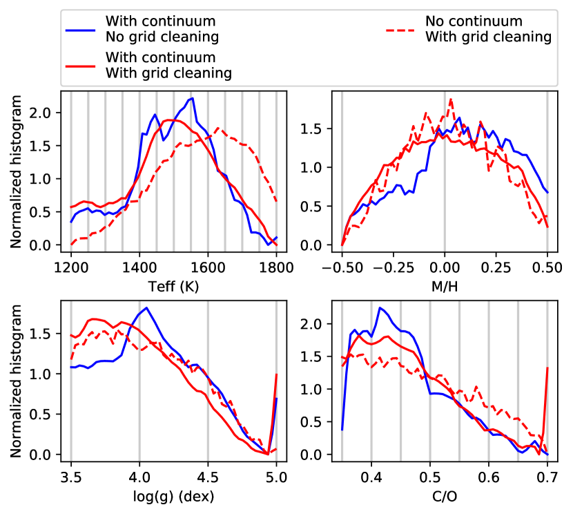
Figure 8: Comparison of posteriors from ForMoSA with different data and models configurations with the grid Exo-REM. In blue : The grid has been taken on the shelf and the continuum has been kept. In red (solid line) : The grid has been cleaned of its non-converged models and the continuum has been kept. In red (dashed line) : The grid has been cleaned of its non-converged models and the continuum has been removed. In grey : The step of the grid for each parameter.

4.1.3 Losing the pseudo-continuum information

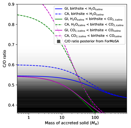
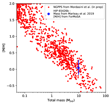
Figure 9: Left: Comparison between the posterior of the C/O ratio given by ForMoSA (gradient; black: high likelihood) and different scenario of formation as a function of the accreted solid mass. The solid lines correspond to the gravitational instability (GI) scenario while the dashed lines correspond to the core accretion (CA) scenario. The blue, green and purple curves represent a formation within the water iceline , between the water and CO₂ icelines and between CO₂ and CO icelines) respectively. Right: Comparison between the bulk enrichment of the NGPPS (red dots) and the estimated properties of HIP 65426 b (blue dot). We show here the NGPPS with a mass higher than 0.05 $\mathrm{M_{Jup}}$  ($\sim$ Neptune’s mass).

The molecular mapping implies a removal of the information contained in the planet spectral continuum. The Figure 8 compares Bayesian posteriors obtained using the grid Exo-REM on the band K with and without the continuum (solid and dashed green line respectively), and the Table 2 summarizes the values of the parameters extracted with error bars. Both approaches yield results in agreement within error bars (1$\sigma$). Nevertheless, the subtraction of the continuum shifts and flattens the $\mathrm{T_{eff}}$  posterior (factor of $\simeq$2.0 between the error bars). The constraint on the other physical parameters is less impacted by the continuum removal, which indicates that the related information is encoded in the line intensities.

These differences clearly point out the limitations of the molecular mapping for constraining the $\mathrm{T_{eff}}$ of objects in the L-type regime from observations at K-band. We still need to investigate if the method, when applied to a different band (J or H-band) or at higher spectral resolution (VLT/ERIS K-band mode at R$\sim$8000, ELT/HARMONI), could retrieve that information.

4.2 Interpreting the radial velocity of HIP 65426 b

An interesting result coming from the SINFONI K-band spectrum of HIP 65426 b is the determination of the radial velocity of the planet itself. As described in Section 2, great care has been taken to calibrate the wavelength dispersion of the cubes using the various telluric absorption lines, and cross-checked at the end with solution found for the OH lines present in the data (centered on zero   km s^-1, see Figure 11). Using both independent approaches, the Bayesian inference and the molecular mapping to measure the radial velocity of HIP 65426 b in the SINFONI datacubes, we find compatible values that give a radial velocity estimate of $21\pm 7$  km s^-1. Similar results are obtained with the molecular mapping approach using the observation acquired on May 25^th, 2018 ($20\pm 8$  km s^-1). We used the molecular mapping technique to estimate the radial velocity on the set of observations acquired on May 26^th, 2018 and we found $31\pm 8$  km s^-1. The radial velocity of both night are consistent at 2-$\mathrm{sigma}$ and we chose to define our final estimate of the radial velocity as RV = $26\pm 15$  km s^-1  to be the most conservative.

A direct application of this result is to check the consistency with the expected Keplerian motion of a bound companion orbiting HIP 65426 A. Considering the orbital solution found for HIP 65426 b by Cheetham et al. (2019), one might expect a maximum difference of $\pm 4.4$  km s^-1  relative to the primary star absolute radial velocity. In the discovery paper of HIP 65426 b, Chauvin et al. (2017) reported for HIP 65426 A a value of $5.2\pm 1.3$  km s^-1, and a very high projected rotational velocity of $v$sin$i=299\pm 9$  km s^-1. They considered for this analysis a set of 14 HARPS spectra acquired during the nights of January 16^th, 17^th and 18^th, 2017, and a two sets of lines: (i) Six strong lines (Ca II K and five H lines from H$\beta$ to H9, excluding H$\epsilon$; using the rotationally broadened core of the lines) and (ii) 35 atomic metallic lines. More details can be found in Appendix B of Chauvin et al. (2017). Given the primary spectral type and its rotational velocity, a precise measurement of the absolute radial velocity is challenging. It motivates to revisit this first analysis mainly focused on the extraction of the stellar rotational velocity. We used this time 78 HARPS spectra obtained during 10 nights spanning a period of time between January, 2017 to March, 2018. We first followed a similar analysis to extract the radial and rotational velocities using both sets of lines (i) and (ii). Although H lines are adapted for the extraction of rotational velocities and the search for variability given their strength, their extended wings makes them less reliable to derive absolute radial velocity as they are more sensitive on the continuum tracing. The revisited absolute radial velocity of HIP 65426 was therefore extracted using only the second set of lines (ii), i.e. the weak metallic lines that are essentially only broadened by the atmospheric velocity field. The resulting radial velocity measurements are shown in Figure 10. A mean radial velocity of $12.2\pm 0.3$   km s^-1  (2.9  km s^-1  for the standard deviation of the RV measurements) is derived, which is significantly different from the value derived by Chauvin et al. (2017), but more reliable given the number of spectra used, the temporal baseline, and the selection of metallic lines more adpated for absolute radial velocity measurements. Moreover, high frequency variation probably related the existence of pulsation are clearly identified. The average value of $v$sin$i$ is lower than originally derived with a value of $261\pm 2$  km s^-1  (16  km s^-1  for the standard deviation of the RV measurements) and no sign of Spectral Binary 1 (SB1) or Spectral Binary 2 (SB2) binary are detected.

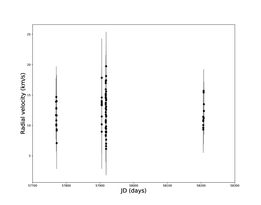
Figure 10: Radial velocity measurements of HIP 65426 using a total of 78 HARPS spectra obtained between 2017 and 2018 at La Silla/3.6m telescope and weak metallic lines less sensitive to the continuum tracing.

From this, we conclude that the difference of radial velocities between HIP 65426 b and A is compatible with a physical object in Keplerian motion (considering the uncertainties on the radial velocities of A and b, and the predicted Keplerian motion for b). We note that the new value of radial velocity measurement of HIP 65426 A is in better agreement with a membership to the LCC subgroup considering the probability predictions of the BANYAN $\Sigma$ code by Gagné et al. (2018). Finally, the direct determination of the radial velocity of imaged exoplanets with medium (to high) resolution spectrographs, as already obtained for $\beta$ Pic b (Snellen et al., 2014), HR 8799 b and c (Ruffio et al., 2019) and now HIP 65426 b, highlights the rich perspective of this technique in synergy with astrometric monitoring to: i/ test the companionship of the newly imaged exoplanetary candidates, ii/ refine their orbital parameters when confirmed, and iii/ measure, with very high spectral spectra, their projected rotational velocity and potentially their spin.

4.3 HIP 65426 b formation pathway

The broad constraints on the C/O ratio and metallicity of HIP 65426 b derived in Section 3 give the opportunity of discussing the planet formation mode. We caution that the C/O ratio estimate depends on the correct assumptions on the cloud prescriptions where grains are efficient oxygen carriers and can impact the composition of the gas phase from which the molecular lines arise (e.g., Helling et al., 2014).

The interpretation relies on several additional hypothesis. The original composition of the putative circumstellar disk where HIP 65426 b may have formed is obviously unknown and the C/O and metallicity of HIP 65426 A, which is a fast rotator (Chauvin et al., 2017), have not been determined either, to our knowledge. Kane et al. (1980) report the C/O ratio of 6 bona-fide members of LCC and UCL but these estimates show a strong dispersion and would need to be revised with the help of recent stellar model atmospheres. Bubar et al. (2011) find on average a sub-solar metallicity ([Fe/H]=-0.12 dex, 0.10 dex rms) for a sample of UCL and LCC solar-type stars. Viana Almeida et al. (2009) report metallicities of $0.02\pm 0.05$ dex and $-0.02\pm 0.09$ dex for 6 and 10 stars from UCL and Upper-Scorpius, respectively. Nissen (2013) reports a correlation between the C/O ratio and the Fe/H of stars with planets with a mean C/O=0.58 at Fe/H=0 (0.06 rms scatter). Therefore, we can expect both HIP 65426A metallicity and C/O ratio to be close to solar values. Yet, the knowledge of the host star composition would be important for strengthening the conclusions on the formation pathway based on the exoplanet atmospheric composition.

Table 3: Imaged planets around intermediate-mass stars with reported abundance measurements

Planet	$a$	Mass	[M/H]	C/O	Refs.
	(au)	($\mathrm{M_{Jup}}$)	(dex)
$\beta$ Pic b	$11^{+0.3}_{-0.4}$	$12.7\pm 2.2$	$0.68^{+0.11}_{-0.08}$	$0.43^{+0.04}_{-0.03}$	1
HR 8799 e	$15.3^{+1.4}_{-1.1}$	$7.2^{+0.6}_{-0.7}$	$0.48^{+0.25}_{-0.29}$	$0.60^{+0.07}_{-0.08}$	2, 3
HR 8799 c	$37.6^{+2.2}_{-1.7}$	$7.2^{+0.6}_{-0.7}$	…	$0.65^{+0.10}_{-0.05}$	2, 4
HR 8799 b	$69.5^{+9.3}_{-7.0}$	$5.8\pm 0.5$	…	$0.61^{+0.09}_{-0.03}$	2, 5
HIP 65426 b	$110^{+90}_{-30}$	$9.9^{+1.1}_{-1.8}$	0.05${}_{-0.22}^{+0.24}$	$\leq$0.55	6, 7, 8

The Gravity Collaboration et al. (2020) have proposed a simple analytical method for interpreting the C/O ratio measured for imaged exoplanets. From the relative abundances of CO, CO₂, H₂O, C (grains) and O (silicates) given in Öberg et al. (2011), they estimated the relative abundance of the C and O in both the solid ($n_{\mathrm{C},\,\mathrm{s}}$, $n_{\mathrm{O},\,\mathrm{s}}$) and gaseous phases ($n_{\mathrm{C},\,\mathrm{g}}$, $n_{\mathrm{O},\,\mathrm{g}}$) and for two possible planet birth locations : within the water iceline and between the water and CO₂ icelines. We considered in addition here the case of a formation between the CO₂ and CO icelines given the projected physical separation of 92 au for HIP 65426 b. The planet birthsite defines $\mathrm{M_{solid}}$  and $\mathrm{M_{gas}}$  as the amount of solid and gas in the atmosphere of the planet and $\mathrm{f_{s/g}}$  the solid/gas ratio in the initial disk to calculate the C/O ratio :

$$\mathrm{C}/\mathrm{O}=\frac{n_{\mathrm{C},\,\mathrm{s}}\,\mathrm{f_{s/g}}\,^{-1}\,\mathrm{M_{solid}}+n_{\mathrm{C},\,\mathrm{g}}\,(1-\mathrm{f_{s/g}})^{-1}\,\mathrm{M_{gas}}}{n_{\mathrm{O},\,\mathrm{s}}\,\mathrm{f_{s/g}}\,^{-1}\,\mathrm{M_{solid}}+n_{\mathrm{O},\,\mathrm{g}}\,(1-\mathrm{f_{s/g}})^{-1}\,\mathrm{M_{gas}}}$$ (1)

In the case of $\mathrm{M_{solid}}$ = $\mathrm{f_{s/g}}$ $\mathrm{M_{planet}}$  and $\mathrm{M_{gas}}$ = (1-$\mathrm{f_{s/g}}$) $\mathrm{M_{planet}}$  where $\mathrm{M_{planet}}$  is the total mass of the planet and $\mathrm{f_{s/g}}$  is assumed to be equal to the standard solid-to-gas ratio of circumstellar disks (0.01), the Equation 1 gives a C/O$\sim$0.55 corresponding to the solar value. During planet formation, this C/O ratio is modified by the accretion of solids and gas. In the case of the gravitational instability scenario, solids are accreted during the sudden collapse ($\mathrm{M_{solid\,ini}}$) and later on through planetesimal accretion ($\mathrm{M_{accreted}}$). Assuming that the total mass accreted during the collapse $\mathrm{M_{ini}}$  $\gg$ $\mathrm{M_{accreted}}$, the total mass of solids in the planet then writes:

$$\mathrm{M_{solid}}\,=\mathrm{f_{s/g}}\,\mathrm{M_{planet}}\,+\,\mathrm{M_{accreted}}$$ (2)

In the case of a formation following a core accretion, $\mathrm{M_{solid}}$ is collected through the slower core accretion process while the gas is brought mostly at the runaway accretion step ($\mathrm{M_{solid}}$  = $\mathrm{M_{accreted}}$). For both scenario, the fraction of the mass of gas in the planet write $\mathrm{M_{gas}}$  = (1 - $\mathrm{f_{s/g}}$) $\mathrm{M_{planet}}$ and that mix is assumed to be representative of the atmospheric composition.

We show in Figure 9 (left) the predictions of the C/O ratio for different values of $\mathrm{M_{solid}}$  and both formation paradigms for a $\mathrm{M_{planet}}$ = 10 $\mathrm{M_{Jup}}$ (Marleau et al., 2019b) planet and birthsites within the water iceline (blue lines), between the water and CO₂ icelines (green lines) and between CO₂ and CO icelines (purple lines). The predictions are compared with the estimate of HIP 65426 b C/O ratio. Both scenarii are consistent with our estimate of C/O ratio.

Kennedy & Kenyon (2008) estimate the water iceline to be originally at $\sim$7 au around a $\sim 2M_{\odot}$ star before moving inward to $\sim$2.5 au at 3 Myr. van der Marel et al. (2019) locate the CO₂ iceline at $\sim 10$ au in the mid-plane of the disks around the $\sim 2M_{\odot}$ young stars V1247 Ori and HD 163296. They also predict CO icelines at $\sim$70 au and $\sim$140 au for these two stars. Qi et al. (2015) report observations of the CO snowline at 75 au around HD 163296 (NB: we revised the published value using the GAIA-DR2 distance of the star) e.g. at shorter separation than the projected physical separation of HIP 65426 b. Therefore, if formed in-situ possibly beyond the CO snowline, the planet must have accreted a substantial amount of solids to lower its C/O ratio.

We caution that these conclusions remain based on a simple approach of planet formation processes and snow lines in disks. The $\mathrm{f_{s/g}}$ might be different than the interstellar value adopted here and is expected to decrease with age due to the growth from micron-sized particles to planetesimals and planets. Ionisation process in the disk can modify drastically the chemical abundances of elements in the region between the H₂O and CO₂ icelines (Eistrup et al., 2018). Furthermore, our 1D approach neglects the variation of the snowline radii at different scale height in the disk (e.g., Dullemond et al., 2020) and their complex evolution in time due to episodic accretion (e.g., Cieza et al., 2016).

The population synthesis approach offers to track down the subtle effects involved in planet formation. The “New Generation Planetary Population Synthesis” (hereafter NGPPS) from the Bern group (Marleau et al., 2019b; Schlecker et al., 2020) predict the bulk enrichment of planets formed by core accretion. They account for type I and II migration, the formation and dynamical interactions of multiple planet embryos per disk. The population has not yet been computed for a host-star more massive than 1.5 $\mathrm{M_{\odot}}$. However, the predictions of bulk enrichment for the populations of planets around 1.0 and 1.5 $\mathrm{M_{\odot}}$ show not significant change and we therefore assume here that it remains valid for a 2 $\mathrm{M_{\odot}}$ star such as HIP 65426 A.

At an age of 10 Myr, the simulation contains $\sim$ 24500 bodies with masses up to 65.9 $\mathrm{M_{Jup}}$ and semi-major axis out to $\sim 800$ au. The solar-metallicity of HIP 65426 b is well compatible with the bulk metallicity of the NGPPS planets in the same mass range (Figure 9) but the simulated planets are found on much tighter orbits (semi-major axis from 0.57 to 11.16 au for planets in the same ranges of mass and metallicity than HIP 65426 b) than the projected separation of HIP 65426 b (92 au). The conclusions remain unchanged at 20 Myr. This comparison of the atmospheric metallicity and bulk enrichment assumes that the metals acquired at formation get diluted in the planet envelop.

To conclude, the abundances of HIP 65426 b can be compared to those of imaged companions around the intermediate-mass stars with similar measurements (Table 3). The C/O ratio and mass of HIP 65426 b are reminiscent of $\beta$ Pictoris b located much closer to its host star at 11 au. This supports the above hypothesis on the formation of the planet closer in, then scattered at larger separation via planet-planet interactions (see Marleau et al. 2019a). Such hypothesis could also explain the different separations observed between HIP 65426 b and the NGPPS population at the same mass, age, and metallicity ranges. A future refinement of the orbital parameters with GRAVITY will help clarifying the dynamical history of the planet and the interpretation of the planet composition derived here.

5 Summary and conclusions

We analysed new K-band medium-resolution IFS data obtained with SINFONI at VLT of the HIP 65426 b exoplanet, discovered by SPHERE, to further characterize its atmosphere. Our TExTRIS python analysis toolkit for IFS data was able to retrieve the star position outside the field of view and to optimise the data processing allowing for the extraction of the planet emission spectrum. We interpreted this spectrum following a Bayesian inference with self-consistent atmospheric forward models with the ForMoSA code (Petrus et al., 2020) and compared the inferred atmospheric properties of the planet to those obtained from the recent “molecular mapping” technique based on cross-correlation between the IFS data elements and grid of models. We can summarize the main results as follows:

1. We find a $\mathrm{T_{eff}}$=1560$\pm 100$K, log g$\leq$4.40 dex, [M/H]=$0.05^{+0.24}_{-0.22}$ dex, and C/O $\leq$0.55 from ForMoSA. The accuracy is limited by the systematic uncertainties induced by the use of different models and by the bi-modal distribution of solutions found with the BT-SETTL15 models. That composition is consistent with a formation of HIP 65426 b closer to the host-star by core-accretion. We can not exclude a formation by gravitational instability at large separation, but the latter would imply the accretion of a substantial amount of solids.

2. The molecular mapping as performed with TExTRIS yields results consistent with the ones from ForMoSA that validates the ability of the molecular mapping to characterize atmospheres. Nevertheless, this alternative method is limited by the loss of the spectral continuum information in the data that can shift the estimates of $\mathrm{T_{eff}}$, and degrades the constraints on the other parameters (log(g), [M/H], C/O).

3. We estimated a radial velocity of 26$\pm$15   km s^-1  for the planet compatible with the revised radial velocity of the host-star. This highlights the usefulness of medium (to high) resolution spectrographs to test companionship.

GRAVITY observations could soon drastically improve the knowledge of the orbital parameter of the planet and potentially draw a consistent picture of its formation. Observations with ERIS and CRIRES+ would also allow for improving the knowledge of the radial velocity and consolidate the constraints on the atmospheric parameters derived from our K-band data.

A new generation of integral field spectrographs successor of SINFONI (VLT-ERIS, GTC-FRIDA, JWST-NIRSpec and MIRI, ELT-HARMONI and METIS) will soon observe at high-Strehls, higher spectral resolution (up to $R_{\lambda}\sim$100 000 for METIS) and high-contrast (GTC-FRIDA, HARMONI-high contrast arm; METIS). All these instruments belong to the same class of slicer-based IFS and present similar challenges in terms of data analysis. The techniques developed and explored as part of this study could be adapted to process these observations.

Appendix A Robustness of the wavelength solution at the companion location

We checked the accuracy of the correction we applied on the wavelength solution of the instrument using OH^- emission lines. Seventeen lines from 1.977 to 2.23 $\mathrm{\mu m}$  are well detected in the stacked cubes (e.g., Figure 1) on both nights. Their central wavelength at the companion location could therefore be determined with an average accuracy of 3.5   km s^-1  using a Gaussian fit and be compared to reference values from Rousselot et al. (2000). The residual shifts are reported in Figure 11 and oscillates around means of 2.3 and 2.8   km s^-1, for the May 25 and 26 data, respectively. These values and the measurement accuracy indicate no significant residual wavelength shift and validate locally our re-calibration based on telluric absorption.

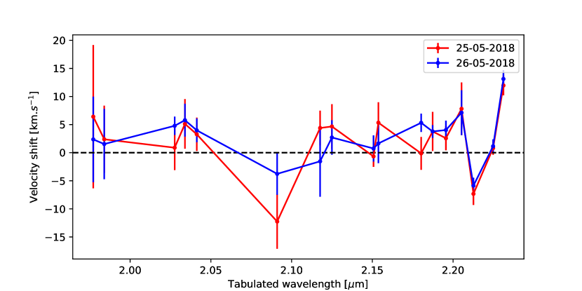
Figure 11: Velocity shifts between the measured and tabulated positions (vacuum) of OH lines at the position of the companion in the stacked datacubes.

Appendix B Validating the extraction procedure

We tested the different extraction methods described in section 2 injecting a fake planet with a K-band contrast of 10 magnitudes (corresponding to the values reported in Cheetham et al., 2019) and a position angle of 165.2^∘. The fake planet spectrum was extracted within a 75mas wide circular aperture and compared to the injected signal. The results are shown for both nights in Figure 12.

The test confirms the ability of the PCA to conserve the continuum shape. Conversely, the removal of the circular profile in the nADI cubes leaves large-scale flux halo residuals which introduce a bias of the continuum at the fake planet location. The 2D-polynomials applied on these cubes remove these residuals efficiently at shorter wavelengths, but bias the pseudo-continuum longward of 2.3 $\mathrm{\mu m}$. We estimated the signal-to-noise (S/N) from the difference of the normalised extracted and injected spectra. The signal-to-noise is systematically lower using the PCA. We therefore conclude that the PCA conserves the planet continuum information, but is not optimised for accessing the molecular lines.

We show in Figure 13 the flux-calibrated spectrum of HIP 65426b. The PCA-extracted spectra obtained from the May 25 and 26 datacubes and the one extracted from the May 25 nADI cubes show identical continua, confirming the later method works better at the planet position. The PCA spectrum is noisier than the nADI spectrum, in agreement with the conclusions based on fake planets. The combination of the two PCA-extracted spectra of HIP 65426b does not reach the signal-to-noise obtained from the nADI/polynomial fit from the May 25 data. We therefore adopted the spectrum extracted from the nADI and polynomial fit. The final flux-calibrated spectrum of HIP 65426b appears to be consistent with the SPHERE K-band photometry.

To conclude, we tested different square box sizes (10, 15, 20, 25 pixels width) as well as different degrees (1 to 5) of polynomials when applying the background correction to the nADI cubes. The results are shown in Figure 14 for the May 25, 2018 observations. Boxes smaller than 15 pixels do not contain enough spaxels to evaluate the background and lead to noisier spectra. Boxes larger than 20 pixels encompass artefacts at the edges of the field of view of SINFONI and were discarded. Square boxes of 15 and 20 pixels width yield similar results. We chose the later to allow for estimating the level of residuals within an annuli of 53mas width (e.g., a resolution element) centered on the planet. Polynomials of degree 2 to 5 produce spectra with identical continua. The S/N decreases when higher degrees are considered. Polynomials of degree 1 seem to optimise the S/N ratio. However, it leaves a higher level of residuals around the planet and does not subtract the continuum properly at shorter wavelengths. Therefore, we concluded that a box-size of 20 pixels and a polynomials of degree 2 is the best trade-off on these data.

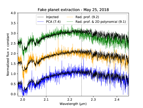
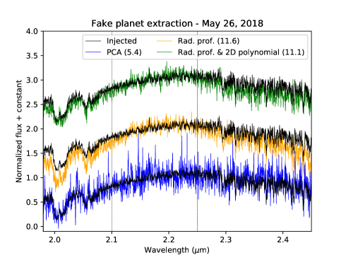
Figure 12: Comparison of the injected (black lines) and extracted fake planet spectra (color lines) using the methods described in Section 2: the principal-component analysis (blue), the removal of a circular profile at each wavelengths (orange), and the removal of a 2D polynomials at each wavelengths at the fake planet position (green). The signal-to-noise ratio of the recovered spectra is computed from 2.1 to 2.25 $\mu$m (dashed vertical lines) and given in parenthesis.

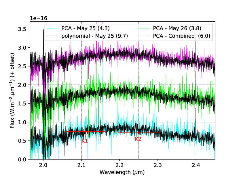
Figure 13: Flux-calibrated spectra of HIP 65426b obtained with the PCA on both nights and compared to the spectrum extracted from the nADI reduction of the May 25, 2018 data followed by a subtraction of a 2D polynomials. The signal-to-noise ratio (S/N) estimated from 2.1 to 2.25 $\mu$m is given in parenthesis. The red datapoints correspond to the SPHERE K1 and K2 photometry from Cheetham et al. (2019).

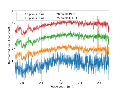
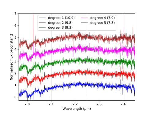
Figure 14: Extracted spectra (with telluric features) of HIP 65426b for different box sizes (left) and degree (right) of the polynomial fit applied to the nADI data. The signal-to-noise ratio (S/N) of the spectra estimated from 2.1 to 2.25 $\mu$m is given in parenthesis.

Appendix C Detection of planets with different C/O ratio with the CO molecular template.

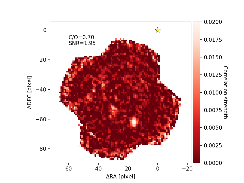
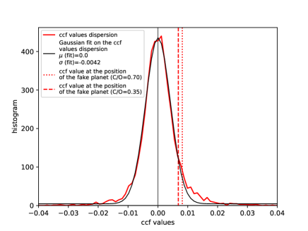
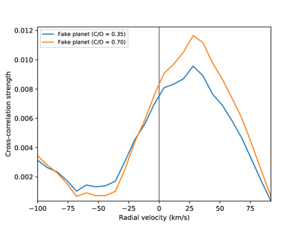
Figure 15: Upper-Left and Right: CO molecular maps obtained following the injection of a fake planet at $\rho$=812 mas and PA=165.2^∘ in the original data-cubes using Exo-REM models at $\mathrm{T_{eff}}$=1650 K, log(g)=4.0 dex, [M/H]=0.0, and C/O=0.35 and 0.70 at a velocity of 30   km s^-1. Bottom-left Histograms of CCF values at a velicity of 30   km s^-1. Bottom-right Cross-correlation function obtained at the fake planet position.

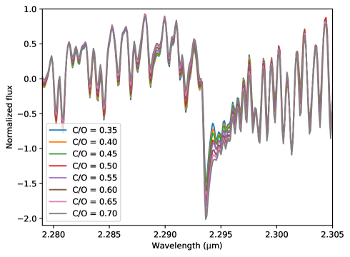
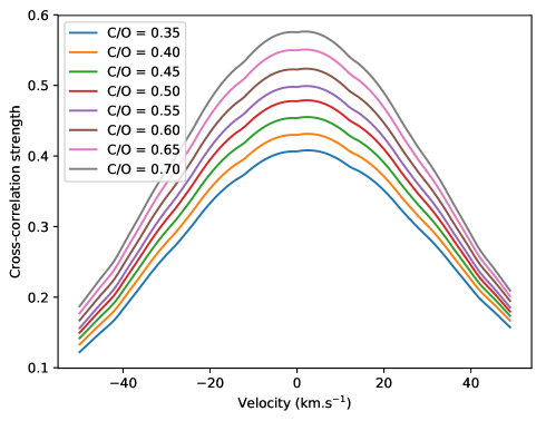
Figure 16: Left : Zoom on the $\nu=$2–0 CO overtone at 2.29 $\mathrm{\mu m}$  of normalized continuum-subtracted Exo-REM models at different C/O ratios ($\mathrm{T_{eff}}$=1650 K, log(g)=0.40 dex, [M/H]=0.0 and C/O=0.35-0.70). Right : cross-correlation functions between the Exo-REM models and the CO template shown in Figure 4.

We investigated in the following the faint detection of HIP 65426b using the CO molecular template. We injected fake planets (FP hereafter) into our datacube and compared the detection S/N into the CCF signal maps generated for each cases. The fake planets were injected at $\rho$=812 mas, PA=165.2^∘, a broad-band contrast $\Delta_{K}$=10 mag, and a radial velocity RV=30   km s^-1. We used a noiseless synthetic spectrum generated with the Exo-REM model corresponding to a $\mathrm{T_{eff}}$=1650 K, a log(g)=4.0 dex, a [M/H]=0.0 and a C/O=0.35 and 0.70 for each FP respectively. The Figure 15 shows the cross-correlation function for each FP obtain following the method described in Section 3.3.1. The signal is detected at a larger S/N than on for the real planet which might be due to the lack of noise in the injected spectral signature. The comparison however shows that planets with low C/O such as HIP 65426b are detected at a lower S/N than planets with super-solar C/O. Indeed, the Exo-REM models predict a less pronounced $\nu=$2–0 overtone, which is the strongest spectroscopic signature of ¹²CO in the spectrum (see also Fig. 4). This translates to a reduced cross-correlation signal (Figure 16). This may therefore explain in part the marginal detection of HIP 65426b with the CO molecular template.

References

- Abuter et al. (2006) Abuter, R., Schreiber, J., Eisenhauer, F., et al. 2006, New A Rev., 50, 398
- Ackerman & Marley (2001) Ackerman, A. S. & Marley, M. S. 2001, ApJ, 556, 872
- Allard et al. (2001) Allard, F., Hauschildt, P. H., Alexander, D. R., Tamanai, A., & Schweitzer, A. 2001, ApJ, 556, 357
- Allard et al. (2012) Allard, F., Homeier, D., & Freytag, B. 2012, Philosophical Transactions of the Royal Society of London Series A, 370, 2765
- Astropy Collaboration et al. (2018) Astropy Collaboration, Price-Whelan, A. M., SipHocz, B. M., et al. 2018, aj, 156, 123
- Bailey et al. (2014) Bailey, V., Meshkat, T., Reiter, M., et al. 2014, ApJ, 780, L4
- Baraffe et al. (2003) Baraffe, I., Chabrier, G., Barman, T. S., Allard, F., & Hauschildt, P. H. 2003, A&A, 402, 701
- Barman et al. (2015) Barman, T. S., Konopacky, Q. M., Macintosh, B., & Marois, C. 2015, ApJ, 804, 61
- Barman et al. (2011) Barman, T. S., Macintosh, B., Konopacky, Q. M., & Marois, C. 2011, ApJ, 733, 65
- Bayo et al. (2008) Bayo, A., Rodrigo, C., Barrado Y Navascués, D., et al. 2008, A&A, 492, 277
- Becklin & Zuckerman (1988) Becklin, E. E. & Zuckerman, B. 1988, Nature, 336, 656
- Beuzit et al. (2019) Beuzit, J. L., Vigan, A., Mouillet, D., et al. 2019, A&A, 631, A155
- Boley et al. (2011) Boley, A. C., Helled, R., & Payne, M. J. 2011, ApJ, 735, 30
- Bonnefoy et al. (2013) Bonnefoy, M., Boccaletti, A., Lagrange, A. M., et al. 2013, A&A, 555, A107
- Bonnefoy et al. (2014) Bonnefoy, M., Chauvin, G., Lagrange, A. M., et al. 2014, A&A, 562, A127
- Bonnefoy et al. (2016) Bonnefoy, M., Zurlo, A., Baudino, J. L., et al. 2016, A&A, 587, A58
- Bonnet et al. (2004) Bonnet, H., Abuter, R., Baker, A., et al. 2004, The Messenger, 117, 17
- Bowler & Hillenbrand (2015) Bowler, B. P. & Hillenbrand, L. A. 2015, ApJ, 811, L30
- Bowler et al. (2017) Bowler, B. P., Kraus, A. L., Bryan, M. L., et al. 2017, AJ, 154, 165
- Bowler et al. (2010) Bowler, B. P., Liu, M. C., Dupuy, T. J., & Cushing, M. C. 2010, ApJ, 723, 850
- Bowler et al. (2011) Bowler, B. P., Liu, M. C., Kraus, A. L., Mann, A. W., & Ireland, M. J. 2011, ApJ, 743, 148
- Briechle & Hanebeck (2001) Briechle, K. & Hanebeck, U. D. 2001, in Optical Pattern Recognition XII, ed. D. P. Casasent & T.-H. Chao, Vol. 4387, International Society for Optics and Photonics (SPIE), 95 – 102
- Brogi & Line (2019) Brogi, M. & Line, M. R. 2019, AJ, 157, 114
- Bubar et al. (2011) Bubar, E. J., Schaeuble, M., King, J. R., Mamajek, E. E., & Stauffer, J. R. 2011, AJ, 142, 180
- Carlotti et al. (2018) Carlotti, A., Hénault, F., Dohlen, K., et al. 2018, in Society of Photo-Optical Instrumentation Engineers (SPIE) Conference Series, Vol. 10702, Proc. SPIE, 107029N
- Chabrier et al. (2000) Chabrier, G., Baraffe, I., Allard, F., & Hauschildt, P. 2000, ApJ, 542, 464
- Charnay et al. (2018) Charnay, B., Bézard, B., Baudino, J. L., et al. 2018, ApJ, 854, 172
- Chauvin et al. (2017) Chauvin, G., Desidera, S., Lagrange, A. M., et al. 2017, A&A, 605, L9
- Chauvin et al. (2018) Chauvin, G., Gratton, R., Bonnefoy, M., et al. 2018, A&A, 617, A76
- Chauvin et al. (2005) Chauvin, G., Lagrange, A. M., Zuckerman, B., et al. 2005, A&A, 438, L29
- Cheetham et al. (2019) Cheetham, A. C., Samland, M., Brems, S. S., et al. 2019, A&A, 622, A80
- Chilcote et al. (2017) Chilcote, J., Pueyo, L., De Rosa, R. J., et al. 2017, AJ, 153, 182
- Christiaens et al. (2019) Christiaens, V., Cantalloube, F., Casassus, S., et al. 2019, ApJ, 877, L33
- Cieza et al. (2016) Cieza, L. A., Casassus, S., Tobin, J., et al. 2016, Nature, 535, 258
- Cutri & et al. (2012) Cutri, R. M. & et al. 2012, VizieR Online Data Catalog, II/311
- Cutri et al. (2003) Cutri, R. M., Skrutskie, M. F., van Dyk, S., et al. 2003, VizieR Online Data Catalog, II/246
- Daemgen et al. (2017) Daemgen, S., Todorov, K., Quanz, S. P., et al. 2017, A&A, 608, A71
- Davies (2007) Davies, R. I. 2007, MNRAS, 375, 1099
- De Rosa et al. (2016) De Rosa, R. J., Rameau, J., Patience, J., et al. 2016, ApJ, 824, 121
- de Zeeuw et al. (1999) de Zeeuw, P. T., Hoogerwerf, R., de Bruijne, J. H. J., Brown, A. G. A., & Blaauw, A. 1999, AJ, 117, 354
- Delorme et al. (2017) Delorme, P., Schmidt, T., Bonnefoy, M., et al. 2017, A&A, 608, A79
- DENIS Consortium (2005) DENIS Consortium. 2005, VizieR Online Data Catalog, II/263
- Dullemond et al. (2020) Dullemond, C. P., Isella, A., Andrews, S. M., Skobleva, I., & Dzyurkevich, N. 2020, A&A, 633, A137
- Eisenhauer et al. (2003) Eisenhauer, F., Abuter, R., Bickert, K., et al. 2003, Society of Photo-Optical Instrumentation Engineers (SPIE) Conference Series, Vol. 4841, SINFONI - Integral field spectroscopy at 50 milli-arcsecond resolution with the ESO VLT, ed. M. Iye & A. F. M. Moorwood, 1548–1561
- Eistrup et al. (2018) Eistrup, C., Walsh, C., & van Dishoeck, E. F. 2018, A&A, 613, A14
- Freudling et al. (2013) Freudling, W., Romaniello, M., Bramich, D. M., et al. 2013, A&A, 559, A96
- Gagné et al. (2018) Gagné, J., Mamajek, E. E., Malo, L., et al. 2018, ApJ, 856, 23
- Gaia Collaboration et al. (2016) Gaia Collaboration, Brown, A. G. A., Vallenari, A., et al. 2016, A&A, 595, A2
- Gonzalez et al. (2017) Gonzalez, C. A. G., Wertz, O., Absil, O., et al. 2017, The Astronomical Journal, 154, 7
- Gravity Collaboration et al. (2020) Gravity Collaboration, Nowak, M., Lacour, S., et al. 2020, A&A, 633, A110
- Greenbaum et al. (2018) Greenbaum, A. Z., Pueyo, L., Ruffio, J.-B., et al. 2018, AJ, 155, 226
- Groff et al. (2015) Groff, T. D., Kasdin, N. J., Limbach, M. A., et al. 2015, Society of Photo-Optical Instrumentation Engineers (SPIE) Conference Series, Vol. 9605, The CHARIS IFS for high contrast imaging at Subaru, 96051C
- Hauschildt et al. (1997) Hauschildt, P. H., Baron, E., & Allard, F. 1997, ApJ, 483, 390
- Helling et al. (2008) Helling, C., Ackerman, A., Allard, F., et al. 2008, MNRAS, 391, 1854
- Helling et al. (2014) Helling, C., Woitke, P., Rimmer, P. B., et al. 2014, Life, 4, 142
- Hoeijmakers et al. (2018) Hoeijmakers, H. J., Schwarz, H., Snellen, I. A. G., et al. 2018, A&A, 617, A144
- Høg et al. (2000) Høg, E., Fabricius, C., Makarov, V. V., et al. 2000, A&A, 355, L27
- Hubeny & Burrows (2007) Hubeny, I. & Burrows, A. 2007, ApJ, 669, 1248
- Hunter (2007) Hunter, J. D. 2007, Computing in Science & Engineering, 9, 90
- Janson et al. (2010) Janson, M., Bergfors, C., Goto, M., Brandner, W., & Lafrenière, D. 2010, ApJ, 710, L35
- Janson et al. (2008) Janson, M., Brandner, W., & Henning, T. 2008, A&A, 478, 597
- Jones, A. et al. (2013) Jones, A., Noll, S., Kausch, W., Szyszka, C., & Kimeswenger, S. 2013, A&A, 560, A91
- Jovanovic et al. (2015) Jovanovic, N., Martinache, F., Guyon, O., et al. 2015, PASP, 127, 890
- Kane et al. (1980) Kane, L., McKeith, C. D., & Dufton, P. L. 1980, A&A, 84, 115
- Kanodia & Wright (2018a) Kanodia, S. & Wright, J. 2018a, Research Notes of the American Astronomical Society, 2, 4
- Kanodia & Wright (2018b) Kanodia, S. & Wright, J. T. 2018b, Barycorrpy: Barycentric velocity calculation and leap second management
- Kennedy & Kenyon (2008) Kennedy, G. M. & Kenyon, S. J. 2008, ApJ, 673, 502
- Konopacky et al. (2013) Konopacky, Q. M., Barman, T. S., Macintosh, B. A., & Marois, C. 2013, Science, 339, 1398
- Lafrenière et al. (2008) Lafrenière, D., Jayawardhana, R., & van Kerkwijk, M. H. 2008, ApJ, 689, L153
- Lavie et al. (2017) Lavie, B., Mendonça, J. M., Mordasini, C., et al. 2017, AJ, 154, 91
- Lavigne et al. (2009) Lavigne, J.-F., Doyon, R., Lafrenière, D., Marois, C., & Barman, T. 2009, ApJ, 704, 1098
- Lodders (2010) Lodders, K. 2010, Astrophysics and Space Science Proceedings, 16, 379
- Lodieu et al. (2018) Lodieu, N., Zapatero Osorio, M. R., Béjar, V. J. S., & Peña Ramírez, K. 2018, MNRAS, 473, 2020
- Macintosh et al. (2006) Macintosh, B., Graham, J., Palmer, D., et al. 2006, Society of Photo-Optical Instrumentation Engineers (SPIE) Conference Series, Vol. 6272, The Gemini Planet Imager, 62720L
- Madhusudhan et al. (2011) Madhusudhan, N., Burrows, A., & Currie, T. 2011, ApJ, 737, 34
- Manjavacas et al. (2014) Manjavacas, E., Bonnefoy, M., Schlieder, J. E., et al. 2014, A&A, 564, A55
- Marleau et al. (2019a) Marleau, G.-D., Coleman, G. A. L., Leleu, A., & Mordasini, C. 2019a, A&A, 624, A20
- Marleau et al. (2019b) Marleau, G.-D., Coleman, G. A. L., Leleu, A., & Mordasini, C. 2019b, A&A, 624, A20
- Marley et al. (2012) Marley, M. S., Saumon, D., Cushing, M., et al. 2012, ApJ, 754, 135
- Marois et al. (2006) Marois, C., Lafrenière, D., Doyon, R., Macintosh, B., & Nadeau, D. 2006, ApJ, 641, 556
- Marois et al. (2008) Marois, C., Macintosh, B., Barman, T., et al. 2008, Science, 322, 1348
- McElwain et al. (2007) McElwain, M. W., Metchev, S. A., Larkin, J. E., et al. 2007, ApJ, 656, 505
- Mesa et al. (2019) Mesa, D., Bonnefoy, M., Gratton, R., et al. 2019, A&A, 624, A4
- Mesa et al. (2020) Mesa, D., D’Orazi, V., Vigan, A., et al. 2020, MNRAS, 495, 4279
- Meshkat et al. (2015) Meshkat, T., Bonnefoy, M., Mamajek, E. E., et al. 2015, MNRAS, 453, 2378
- Mohanty et al. (2007) Mohanty, S., Jayawardhana, R., Huélamo, N., & Mamajek, E. 2007, ApJ, 657, 1064
- Mollière et al. (2020) Mollière, P., Stolker, T., Lacour, S., et al. 2020, arXiv e-prints, arXiv:2006.09394
- Mollière et al. (2019) Mollière, P., Wardenier, J. P., van Boekel, R., et al. 2019, A&A, 627, A67
- Mordasini (2013) Mordasini, C. 2013, A&A, 558, A113
- Mordasini et al. (2016) Mordasini, C., van Boekel, R., Mollière, P., Henning, T., & Benneke, B. 2016, ApJ, 832, 41
- Morley et al. (2012) Morley, C. V., Fortney, J. J., Marley, M. S., et al. 2012, ApJ, 756, 172
- Moses et al. (2016) Moses, J. I., Marley, M. S., Zahnle, K., et al. 2016, ApJ, 829, 66
- Nakajima et al. (1995) Nakajima, T., Oppenheimer, B. R., Kulkarni, S. R., et al. 1995, Nature, 378, 463
- N’Diaye et al. (2018) N’Diaye, M., Cuevas, S., Sánchez, B., et al. 2018, in Society of Photo-Optical Instrumentation Engineers (SPIE) Conference Series, Vol. 10703, Proc. SPIE, 107033E
- Nissen (2013) Nissen, P. E. 2013, A&A, 552, A73
- Noll, S. et al. (2012) Noll, S., Kausch, W., Barden, M., et al. 2012, A&A, 543, A92
- Nowak et al. (2019) Nowak, M., Lacour, S., Mollière, P., Wang, J., & Charnay, B. 2019, in AAS/Division for Extreme Solar Systems Abstracts, Vol. 51, AAS/Division for Extreme Solar Systems Abstracts, 404.07
- Öberg & Bergin (2016) Öberg, K. I. & Bergin, E. A. 2016, ApJ, 831, L19
- Öberg et al. (2011) Öberg, K. I., Murray-Clay, R., & Bergin, E. A. 2011, ApJ, 743, L16
- Patience et al. (2010) Patience, J., King, R. R., de Rosa, R. J., & Marois, C. 2010, A&A, 517, A76
- Petit dit de la Roche et al. (2018) Petit dit de la Roche, D. J. M., Hoeijmakers, H. J., & Snellen, I. A. G. 2018, A&A, 616, A146
- Petrus et al. (2020) Petrus, S., Bonnefoy, M., Chauvin, G., et al. 2020, A&A, 633, A124
- Qi et al. (2015) Qi, C., Öberg, K. I., Andrews, S. M., et al. 2015, ApJ, 813, 128
- Rajan et al. (2017) Rajan, A., Rameau, J., De Rosa, R. J., et al. 2017, AJ, 154, 10
- Rajpurohit et al. (2018) Rajpurohit, A. S., Allard, F., Rajpurohit, S., et al. 2018, A&A, 620, A180
- Rizzuto et al. (2011) Rizzuto, A. C., Ireland, M. J., & Robertson, J. G. 2011, MNRAS, 416, 3108
- Rousselot et al. (2000) Rousselot, P., Lidman, C., Cuby, J. G., Moreels, G., & Monnet, G. 2000, A&A, 354, 1134
- Ruffio et al. (2019) Ruffio, J.-B., Macintosh, B., Konopacky, Q. M., et al. 2019, AJ, 158, 200
- Samland et al. (2017) Samland, M., Mollière, P., Bonnefoy, M., et al. 2017, A&A, 603, A57
- Schlecker et al. (2020) Schlecker, M., Mordasini, C., Emsenhuber, A., et al. 2020, arXiv e-prints, arXiv:2007.05563
- Schmidt et al. (2014) Schmidt, T. O. B., Mugrauer, M., Neuhäuser, R., et al. 2014, A&A, 566, A85
- Schmidt et al. (2008) Schmidt, T. O. B., Neuhäuser, R., Seifahrt, A., et al. 2008, A&A, 491, 311
- Seifahrt et al. (2007) Seifahrt, A., Neuhäuser, R., & Hauschildt, P. H. 2007, A&A, 463, 309
- Skemer et al. (2014) Skemer, A. J., Marley, M. S., Hinz, P. M., et al. 2014, ApJ, 792, 17
- Skilling (2006) Skilling, J. 2006, Bayesian Anal., 1, 833
- Snellen et al. (2014) Snellen, I. A. G., Brandl, B. R., de Kok, R. J., et al. 2014, Nature, 509, 63
- Sparks & Ford (2002) Sparks, W. B. & Ford, H. C. 2002, ApJ, 578, 543
- Stone et al. (2016) Stone, J. M., Eisner, J., Skemer, A., et al. 2016, ApJ, 829, 39
- Thatte et al. (2007) Thatte, N., Abuter, R., Tecza, M., et al. 2007, MNRAS, 378, 1229
- Trotta (2008) Trotta, R. 2008, Contemporary Physics, 49, 71
- Uyama et al. (2020) Uyama, T., Currie, T., Hori, Y., et al. 2020, AJ, 159, 40
- Valletta & Helled (2018) Valletta, C. & Helled, R. 2018, arXiv e-prints, arXiv:1811.10904
- van der Marel et al. (2019) van der Marel, N., Dong, R., di Francesco, J., Williams, J. P., & Tobin, J. 2019, ApJ, 872, 112
- Viana Almeida et al. (2009) Viana Almeida, P., Santos, N. C., Melo, C., et al. 2009, A&A, 501, 965
- Wang et al. (2018) Wang, J. J., Graham, J. R., Dawson, R., et al. 2018, AJ, 156, 192