Simulating hydrodynamics on noisy intermediate-scale quantum devices with random circuits

Abstract

In a recent milestone experiment, Google’s processor Sycamore heralded the era of “quantum supremacy” by sampling from the output of (pseudo-)random circuits. We show that such random circuits provide tailor-made building blocks for simulating quantum many-body systems on noisy intermediate-scale quantum (NISQ) devices. Specifically, we propose an algorithm consisting of a random circuit followed by a trotterized Hamiltonian time evolution to study hydrodynamics and to extract transport coefficients in the linear response regime. We numerically demonstrate the algorithm by simulating the buildup of spatiotemporal correlation functions in one- and two-dimensional quantum spin systems, where we particularly scrutinize the inevitable impact of errors present in any realistic implementation. Importantly, we find that the hydrodynamic scaling of the correlations is highly robust with respect to the size of the Trotter step, which opens the door to reach nontrivial time scales with a small number of gates. While errors within the random circuit are shown to be irrelevant, we furthermore unveil that meaningful results can be obtained for noisy time evolutions with error rates achievable on near-term hardware. Our work emphasizes the practical relevance of random circuits on NISQ devices beyond the abstract sampling task.

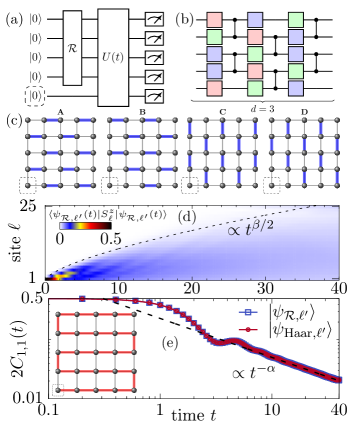
Figure 1: (a) A random circuit ${\cal R}$ acts on $L-1$ qubits, followed by a time evolution $U(t)$ on all $L$ sites. [(b),(c)] ${\cal R}$ comprises $d$ cycles, each composed of layers of one- and two-qubit gates. We consider a 2D geometry and ${\bf A}-{\bf D}$ are patterns of two-qubit gates used in different cycles. [(d),(e)] For reference site $\ell^{\prime}=1$, $\bra{\psi_{{\cal R},\ell^{\prime}}(t)}S_{\ell}^{z}\ket{\psi_{{\cal R},\ell^{\prime}}(t)}$ yields the correlation function $2C_{\ell,1}(t)$. Data is shown for the spin-$1/2$ Heisenberg chain with $L=25$, where the 1D system is realized as a snake-like path through the lattice. Panel (e) shows a cut at $\ell=1$. Even for shallow ${\cal R}$ with $d=20$, results from $\ket{\psi_{{\cal R},\ell^{\prime}}}$ are indistinguishable from a true Haar-random state. Dashed lines indicate power-law scalings of the correlations, cf. Eq. (6).

Introduction. Studying the properties of quantum many-body systems is tremendously challenging Feynman1982 . Notwithstanding significant progress thanks to the development of sophisticated numerical methods schollwoeck20052011 ; weisse2006 ; Verstraete2008 ; Gull2011 ; Aoki2014 ; Carleo2017 and groundbreaking experiments with cold-atom or trapped-ion platforms Bloch2012 ; Blatt2012 , simulations on universal quantum computers promise to yield major advancements in a multitude of research areas Georgescu2014 ; Tacchino2020 . While a fault-tolerant quantum computer is still far into the future, noisy intermediate-scale quantum (NISQ) devices are available and their current capabilities have been demonstrated for various problems such as electronic structure calculations Kandala2017 ; OMalley2016 , simulations of spectral functions Chiesa2019 ; Francis2020 , measurement of entanglement Choo2018 ; Wang2018 , topological phase transitions Smith2019_2 , and out-of-equilibrium dynamics Lamm2018 ; Smith2019 ; Arute2020 ; Sommer2020 .

Recently, an important milestone towards so-called “quantum supremacy” Boixo2018 has been achieved by using Google’s NISQ device Sycamore Arute2019 . In the experiment, the Josephson junction based quantum processor was used to sample from the output distribution of (pseudo-)random circuits involving up to 53 qubits, thereby going beyond the capacities of modern supercomputers. As this sampling task may appear rather abstract, it is crucial to identify a wider range of relevant applications of near-term NISQ devices which can be performed despite their imperfect fidelities of one- and two-qubit gates and the lack of error correction Preskill2018 ; Ippoliti2020 ; Gullans2020 ; Poggi2020 .

Transport processes represent one of the most generic nonequilibrium situations Bertini2020 . In the quantum realm, the understanding of transport not only plays a key role to pave the way for future technologies such as spintronics Wolf2001 , but is also intimately related to fundamental questions of equilibration and thermalization in many-body systems dalessio2016 ; Borgonovi2016 ; Gogolin2016 . While quantum transport has been experimentally studied in mesoscopic systems, solid-state quantum magnets, and cold-atom settings (see e.g. DasSarma2011 ; Hess2019 ; Scheie2020 ; Hild2014 ; Jepsen2020 ), active questions from the theory side include the quantitative calculation of transport coefficients Bertini2020 ; Rakovszky2020 , as well as explaining the emergence of conventional hydrodynamic transport from the underlying unitary time evolution of closed quantum systems Khemani2018 .

In this Letter, we advocate near-term NISQ devices as useful platforms for simulating hydrodynamics in quantum many-body systems and, in particular, we show that random circuits (as realized in Arute2019 ) form tailor-made building blocks for this purpose. With generalizations being possible DeRaedt2000 (see also Supplemental Material SuppMat ), we specifically propose an efficient scheme to compute the infinite-temperature spatiotemporal correlation function $C_{\ell,\ell^{\prime}}(t)$ for one- and two-dimensional (1D, 2D) quantum spin systems,

$$C_{\ell,\ell^{\prime}}(t)=\text{Tr}[S_{\ell}^{z}(t)S_{\ell^{\prime}}^{z}]/2^{L}\ ,$$ (1)

where $S_{\ell(\ell^{\prime})}^{z}$ is a spin-$1/2$ operator at lattice site $\ell$ ($\ell^{\prime}$), $S_{\ell}^{z}(t)=e^{i{\cal H}t}S_{\ell}e^{-i{\cal H}t}$ is the time-evolved operator with respect to (w.r.t.) some Hamiltonian ${\cal H}$, and $L$ denotes the number of spins (qubits). The spatiotemporal correlations $C_{\ell,\ell^{\prime}}(t)$ are central objects for studying transport within linear response theory Bertini2020 , as well as thermalization and many-body localization in quantum systems Luitz2017 . As a key ingredient, our scheme exploits the concept of quantum typicality Popescu2006 ; Goldstein2006 ; Reimann2007 , which asserts that ensemble averages can be accurately approximated by an expectation value w.r.t. a single pure state drawn at random from a high-dimensional Hilbert space Gemmer2004 ; lloydPhd ; bartsch2009 . Remarkably, typicality applies independent of concepts such as the eigenstate thermalization hypothesis dalessio2016 and remains valid also for integrable or many-body localized systems Heitmann2020 .

While random pure states have a long history for efficient numerical simulations Heitmann2020 ; Hams2000 ; iitaka2003 ; Alvarez2008 ; elsayed2013 ; monnai2014 ; steinigeweg2014 ; Richter2019 ; Jin2020 ; Richter2019_2 , we demonstrate in this Letter that typicality can be used to recast the correlation function $C_{\ell,\ell^{\prime}}(t)$ into a form which can be readily evaluated on a quantum computer (see SuppMat for a derivation),

$$C_{\ell,\ell^{\prime}}(t)=\frac{1}{2}\bra{\psi_{{\cal R},\ell^{\prime}}(t)}S_{\ell}^{z}\ket{\psi_{{\cal R},\ell^{\prime}}(t)}+{\cal O}(2^{-L/2})\ ,$$ (2)

where $\ket{\psi_{{\cal R},\ell^{\prime}}(t)}=e^{-i{\cal H}t}\ket{\psi_{{\cal R},\ell^{\prime}}}$, and $\ket{\psi_{{\cal R},\ell^{\prime}}}=\ket{0}_{\ell^{\prime}}\otimes{\cal R}\ket{0}^{\otimes L-1}$ results from the application of a (pseudo-)random circuit ${\cal R}$ on all qubits of the system except for the fixed reference site $\ell^{\prime}$. Importantly, as indicated by the second term on the right-hand side (r.h.s.), the accuracy of Eq. (2) improves exponentially with the size of the system Jin2020 . Complementary to well-known approaches to obtain correlation functions such as Eq. (1) on a quantum computer Terhal2020 ; Somma2002 ; Pedernales2014 (see also Baez2020 ), the scheme proposed in this Letter operates without requiring an overhead of bath or ancilla qubits for initial-state preparation and measurement. Rather, it combines the random-circuit technology already realized on NISQ devices Arute2019 with “quantum parallelism” Alvarez2008 ; Schliemann2002 as the time-evolution of a single random state $\ket{\psi_{{\cal R},\ell^{\prime}}}$ suffices to capture the full ensemble average (1). Furthermore, we particularly scrutinize the impact of Trotter and gate errors present in any realistic implementation and discuss the possibility to extract transport coefficients with error rates achievable on near-term hardware.

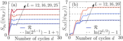
Figure 2: Buildup of randomness of $\ket{\psi_{{\cal R},\ell^{\prime}}}$. (a) $S_{p_{k}}(\ket{\psi_{{\cal R},\ell^{\prime}}})$ reaches the random-state value $\ln(2^{L-1})-1+\gamma$ with Euler constant $\gamma\approx 0.577$ already at moderate $d$ Boixo2018 . (b) $S_{\text{vN}}(\ket{\psi_{{\cal R},\ell^{\prime}}})$ approaches the “Page value” $\ln(2^{L/2})-1$ Page1993 appropriate for a random state on $L-1$ sites. The displayed $L$ values correspond to the 2D geometries $4\times 3$, $4\times 4$, $5\times 4$, and $5\times 5$. Data is averaged over $100$ realizations of ${\cal R}$.

Description of Setup. First, all qubits are initialized in the $\ket{0}$ state. The algorithm then consists of a random circuit ${\cal R}$ acting on $L-1$ qubits followed by a time evolution $U(t)$ on all $L$ sites [Fig. 1 (a)]. ${\cal R}$ comprises individual cycles, each composed of a layer of one-qubit gates and a layer of two-qubit gates, with $d$ denoting the total number of cycles [Fig. 1 (b)]. In each cycle, the one-qubit gates are randomly chosen from the set $\{X^{1/2},Y^{1/2},T\}$, where $X^{1/2}$ ($Y^{1/2}$) are $\pi/2$ rotations around the x-axis (y-axis) of the Bloch sphere and $T$ is the non-Clifford gate $T=\text{diag}(1,e^{i\pi/4})$. We impose the constraint that the one-qubit gates on a given site have to be different in two subsequent cycles. As a two-qubit gate, we consider the controlled-Z (CZ) gate, CZ = $\text{diag}(1,1,1-1)$. (See SuppMat for circuits with CNOT gates.) In each cycle, the CZ gates are aligned in one of the patterns ${\bf A}$-${\bf D}$ on a 2D geometry [Fig. 1 (c)], where we repeat the sequence ${\bf ABCD\dots}$ throughout ${\cal R}$, similar to Refs. Boixo2018 ; Arute2019 . After $d$ cycles, the state $\ket{\psi_{{\cal R},\ell^{\prime}}}=\sum_{k}c_{k}\ket{k}$ is a superposition of computational basis states. It is the important realization that states generated from (shallow) random circuits ${\cal R}$ can approximate the properties of a Haar-random state Emerson2003 ; Oliveira2007 ; Boixo2018 , i.e., the coefficients $c_{k}$ are expected to closely follow a Gaussian distribution with zero mean. (Note that the exact preparation of a Haar-random state would be extremely inefficient in contrast Poulin2011 .)

For the subsequent time evolution, we exemplarily consider the 1D and 2D spin-$1/2$ Heisenberg model with nearest-neighbor interactions (see SuppMat for results on another model Steinigeweg2014_2 ), where we identify $\ket{0}=\ket{\uparrow}$ and $\ket{1}=\ket{\downarrow}$,

$${\cal H}=\sum_{\langle\ell,\ell^{\prime}\rangle}h_{\ell,\ell^{\prime}}=\sum_{\langle\ell,\ell^{\prime}\rangle}{\bf S}_{\ell}\cdot{\bf S}_{\ell^{\prime}}\ ,\quad{\bf S}_{\ell}=(S_{\ell}^{x},S_{\ell}^{y},S_{\ell}^{z})\ ,$$ (3)

where the 1D model is realized as a path through the 2D lattice [Fig. 1 (e)]. Focusing (for now) on 1D, the time-evolution operator $U(t)=\exp(-i{\cal H}t)$ is trotterized DeVries1993 ,

$$U(t)=\left(e^{-i{\cal H}\delta t}\right)^{N}\approx\left(e^{-i{\cal H}_{\text{e}}\delta t}e^{-i{\cal H}_{\text{o}}\delta t}\right)^{N}+{\cal O}(\delta t^{2})\ ,$$ (4)

where ${\cal H}_{\text{e}}$ (${\cal H}_{\text{o}})$ denotes the even (odd) bonds $h_{\ell,\ell^{\prime}}$ of ${\cal H}$, and $\delta t=t/N$ is a discrete time step. The mutually-commuting two-site terms $\exp(-ih_{\ell,\ell^{\prime}}\delta t)$ are then translated into elementary one- and two-qubit gates Tacchino2020 (We here use a representation which requires three CNOT gates Smith2019 ; SuppMat ; Vatan2004 .) Eventually, according to quantum typicality and our construction (see SuppMat ), a $z$-basis measurement of the qubit at site $\ell$ after time $t$ then yields the correlation function $2C_{\ell,\ell^{\prime}}(t)$ [Figs. 1 (d),(e)]. In particular, we show below that the correct extraction of $C_{\ell,\ell^{\prime}}(t)$ remains possible even in the presence of inevitable Trotter and gate errors.

Buildup of randomness. In Fig. 2 (a), we study the growth of $S_{p_{k}}(\ket{\psi_{{\cal R},\ell^{\prime}}})=-\sum_{k=1}^{2^{L}}p_{k}\ln p_{k}$ with $p_{k}=|c_{k}|^{2}$, which measures the spreading of $\ket{\psi_{{\cal R},\ell^{\prime}}}$ within the computational basis due to ${\cal R}$. Moreover, the corresponding entanglement of $\ket{\psi_{{\cal R},\ell^{\prime}}}$ is analyzed in Fig. 2 (b) by means of the von Neumann entropy $S_{\text{vN}}(\ket{\psi_{{\cal R},\ell^{\prime}}})=-\text{Tr}[\rho_{A}\ln\rho_{A}]$, with $\rho_{A}=\text{Tr}_{B}\ket{\psi_{{\cal R},\ell^{\prime}}}\bra{\psi_{{\cal R},\ell^{\prime}}}$ being the reduced density matrix for a half-system bipartition into regions $A$ and $B$. Importantly, we observe that both $S_{p_{k}}$ and $S_{\text{vN}}$ reach their theoretically expected values for a random state Boixo2018 ; Page1993 already at moderate numbers of cycles $d\lesssim 10$, where the required $d$ appears to exhibit only a minor dependence on $L$ Boixo2018 . We thus expect that $\ket{\psi_{{\cal R},\ell^{\prime}}}$ mimics a true Haar-random state even for shallow ${\cal R}$ and can be used within the typicality approach to obtain $C_{\ell,\ell^{\prime}}(t)$. Throughout this Letter, we use a fixed value $d=20$, which yields very accurate results, see Fig. 1 (e) and SuppMat . (Note that $d=20$ has already been realized for $53$ qubits Arute2019 .) Eventually, we stress that this accuracy is achieved even though our design of ${\cal R}$ is not optimized Znidaric2007 ; Weinstein2008 , i.e., no particular fine-tuning of ${\cal R}$ appears to be necessary.

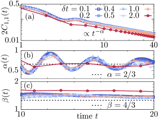
Figure 3: Impact of the Trotter time step. (a) $C_{1,1}(t)$ for varying values of $\delta t$. [(b),(c)] Extracted power-law exponents $\alpha(t)$ and $\beta(t)$. The dashed lines indicate the KPZ scaling Bertini2020 ; Gopalakrishnan2019 ; Ljubotina2017 ; Ljubotina2019 ; Gopalakrishnan2019_2 ; DeNardis2019 ; Weiner2020 . Data is obtained for $L=25$ and $d=20$.

Dependence on Trotter time step. Given the eponymous noise of NISQ devices, it is desirable to use as few gates as possible, i.e., a large time step $\delta t$. However, for a larger $\delta t$, the systematic error of the Trotter decomposition is in turn expected to increase [see r.h.s. of Eq. (4)]. In Fig. 3, we demonstrate that this expectation does not need to hold in practice (see Refs. Heyl2019 ; Sieberer2019 ), such that a favorable trade-off between large $\delta t$ and acceptable Trotter error can be achieved. Specifically, we find that the equal-site correlation function $C_{1,1}(t)$ in Fig. 3 (a) remains almost unchanged for varying $\delta t$ between $\delta t=0.1$ and $\delta t=1$. Even though small deviations appear for larger $\delta t=2$, the qualitative shape of $C_{1,1}(t)$ remains similar also in this case. For a more detailed analysis, we consider the emerging hydrodynamic scaling of $C_{\ell,\ell^{\prime}}(t)$ caused by the conservation of magnetization, $[{\cal H},\sum_{\ell}S_{\ell}^{z}]=0$. In particular, $C_{1,1}(t)\propto t^{-\alpha}$ develops a power-law tail for times $t\gtrsim 10$ [Fig. 3 (a)], while correlations $C_{\ell,1}(t)$ build up throughout the system [cf. Fig. 1 (d)], i.e., $\Sigma^{2}(t)\propto t^{\beta}$ with the spatial variance

$$\Sigma^{2}(t)=\sum_{\ell}\ell^{2}\widetilde{C}_{\ell,1}(t)-\big{[}\sum_{\ell}\ell\widetilde{C}_{\ell,1}(t)\big{]}^{2}\ ,$$ (5)

where $\widetilde{C}_{\ell,1}(t)=C_{\ell,1}(t)/\sum_{\ell=1}^{L}C_{\ell,1}(t)$ with $\sum_{\ell}\widetilde{C}_{\ell,1}(t)=1$. In Figs. 3 (b) and 3 (c), the impact of the Trotter step $\delta t$ on the instantaneous power-law exponents $\alpha(t)$ and $\beta(t)$ is studied for times $10\leq t\leq 20$,

$$\alpha(t)=-\frac{d\ln C_{1,1}(t)}{d\ln t}\ ,\quad\beta(t)=\frac{d\ln\Sigma^{2}(t)}{d\ln t}\ .$$ (6)

We find that $\alpha(t)$ exhibits damped oscillations (presumably caused by the integrability of ${\cal H}$ Gopalakrishnan2019 ) around the mean value $\alpha\approx 2/3$, which signals superdiffusion and is consistent with a description of spin transport in terms of the Kardar-Parisi-Zhang (KPZ) universality class for the integrable and isotropic Heisenberg chain Bertini2020 ; Gopalakrishnan2019 ; Ljubotina2017 ; Ljubotina2019 ; Gopalakrishnan2019_2 ; DeNardis2019 ; Weiner2020 . Remarkably, $\alpha(t)$ is essentially independent of $\delta t$ and $\alpha\approx 2/3$ can be readily extracted even for the largest $\delta t=2$. Likewise, $\beta(t)$ is found to remain stable up to $\delta t\leq 1$, albeit visible deviations now appear for $\delta t=2$, which is explainable by the fact that $\beta(t)$ depends on the accuracy of the Trotter decomposition on the full system while $\alpha(t)$ is a local probe. Overall, the robustness of $C_{\ell,\ell^{\prime}}(t)$ w.r.t. $\delta t$ is an important result and opens the door to reach nontrivial time scales with a manageable number of gates. For instance, fixing $\delta t=1$, an evolution of $L=25$ qubits up to $t=20$ requires $2400$ one-qubit and $1440$ two-qubit gates in our case SuppMat .

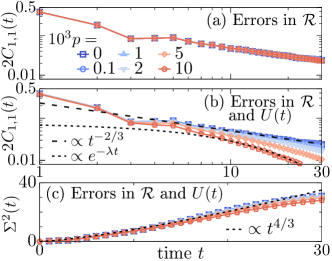
Figure 4: Impact of errors on [(a),(b)] $C_{1,1}(t)$ and (c) $\Sigma^{2}(t)$. In (a) errors are present only within ${\cal R}$. Data is obtained for $L=20$ and $d=20$, averaged over $N_{\bf{r}}=4500$ trajectories for a fixed design of ${\cal R}$ SuppMat .

Impact of noise. To model the impact of erroneous gates, we consider a depolarization model with quantum channels ${\cal E}_{\ell}$ (${\cal E}_{\ell,\ell^{\prime}}$) being applied after each one-qubit (two-qubit) gate Ippoliti2020 ,

$${\cal E}_{\ell}(\rho) =(1-p_{1})\rho+\frac{p_{1}}{3}\sum_{\mu\neq 0}\sigma_{\ell}^{\mu}\rho\sigma_{\ell}^{\mu}\ ,$$ (7)

$${\cal E}_{\ell,\ell^{\prime}}(\rho) =(1-p_{2})\rho+\frac{p_{2}}{15}\sum_{(\mu,\nu)\neq(0,0)}\sigma_{\ell}^{\mu}\sigma_{\ell^{\prime}}^{\nu}\rho\sigma_{\ell}^{\mu}\sigma_{\ell^{\prime}}^{\nu}\ ,$$ (8)

where $\rho$ is the system’s density matrix, $\sigma_{\ell}^{\mu}$ with $\mu=1,2,3$ are Pauli matrices, $\sigma_{\ell}^{0}=\mathbb{1}$, and $p_{1}$ ($p_{2}$) are the one-qubit (two-qubit) error rates. We evaluate Eqs. (7) and (8) by averaging over quantum trajectories Ippoliti2020 ; Dalibard1992 , $\rho(t)\approx(1/N_{\bf{r}})\sum_{\bf{r}}\ket{\psi_{{\cal R},\ell^{\prime}}^{\bf{r}}(t)}\bra{\psi_{{\cal R},\ell^{\prime}}^{\bf{r}}(t)}$, where each trajectory $\ket{\psi_{{\cal R},\ell^{\prime}}^{\bf{r}}(t)}$ corresponds to a particular history of one- and two-qubit Pauli errors. In Figs. 4, we analyze the dynamics of $C_{\ell,\ell^{\prime}}(t)$ obtained for a fixed time step $\delta t=1$ and varying error rates $p=p_{2}=10p_{1}$. First, we consider errors only within ${\cal R}$ and find that they have no effect on the equal-site correlator $C_{1,1}(t)$ [Fig. 4 (a)]. This exemplifies that typicality can also hold for states $\ket{\psi_{{\cal R},\ell^{\prime}}}$ with non-Gaussian distributions of the coefficients $c_{k}$ in the computational basis Jin2020 . Specifically, the distribution of $p_{k}=|c_{k}|^{2}$ drifts from exponential to uniform for large error rates Boixo2018 ; SuppMat . While this has been problematic for the sampling task in Arute2019 , it is irrelevant for our approach.

In contrast, if errors are present in both ${\cal R}$ and $U(t)$ [Fig. 4 (b)], the decay of $C_{1,1}(t)$ depends on $p$. While a power-law tail $C_{1,1}(t)\propto t^{-\alpha}$ with $\alpha=2/3$ can still be extracted for $p\lesssim 2\times 10^{-3}$ (roughly one order of magnitude smaller than currently achievable Arute2019 ), the depolarization errors cause $C_{\ell,\ell^{\prime}}(t)$ to decay exponentially for larger $p$ Ippoliti2020 . Compared to the local probe $C_{1,1}(t)$, the spatial variance $\Sigma^{2}(t)$ appears to be less sensitive to noise, see Fig. 4 (c), and exhibits a power-law growth even for $p=10^{-2}$. The robustness of $\Sigma^{2}(t)$ might be explained by the fact that $\ket{\psi_{{\cal R},\ell^{\prime}}}$ is random and structureless at short times except for sites close to $\ell^{\prime}$. Thus, errors away from $\ell^{\prime}$ do not drastically alter the spreading of $C_{\ell,\ell^{\prime}}(t)$ and the growth of $\Sigma^{2}(t)$. This is another result of this Letter. Given the robustness of $\Sigma^{2}(t)$ [and $C_{\ell,\ell^{\prime}}(t)$] against Trotter and gate errors as well as the gradual improvement of technology, we expect near-term NISQ devices to provide a useful platform to extract transport coefficients, such as diffusion constants, of many-body quantum systems. In this context, the signal-to-noise ratio of the data in actual experiments can be systematically improved by increasing the number of repetitions Arute2019 ; Ippoliti2020 ; SuppMat .

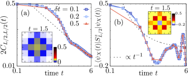
Figure 5: Dynamics in 2D. (a) $C_{L/2,L/2}(t)$ for varying $\delta t$. Dashed line indicates diffusive decay $\propto t^{-1}$. Inset shows $C_{\ell,L/2}(t)$ at $t=1.5$. (b) The nonrandom state $\ket{\psi_{X}(t)}$ (see text for details) yields dynamics incompatible with diffusion.

Dynamics of 2D systems. Our approach is neither restricted to the dynamics of 1D systems nor to the choice of $\ell^{\prime}=1$. In Fig. 5 (a), we repeat our analysis of the $\delta t$ dependence for a 2D Heisenberg model with $L=L_{x}\times L_{y}=25$ and choose the reference site $\ell^{\prime}=L/2$ as the central site of the lattice. Analogous to the 1D case, we find that $C_{L/2,L/2}(t)$ is remarkably robust w.r.t. $\delta t$, with a stable hydrodynamic tail $C_{L/2,L/2}(t)\propto t^{-1}$, which signals the onset of conventional diffusion in 2D consistent with the transition from integrability to nonintegrability of ${\cal H}$ from 1D to 2D Bertini2020 . Finally, let us consider the state $\ket{\psi_{X}}=\ket{\rightarrow}^{\otimes L/2-1}\otimes\ket{\uparrow}\otimes\ket{\rightarrow}^{\otimes L/2}$, i.e., a nonrandom product state where spins at $\ell\neq\ell^{\prime}$ point in the $x$ direction, preparable by applying Hadamard gates on all but the central site. At $t=0$, this state yields $\bra{\psi_{X}}S_{\ell}^{z}\ket{\psi_{X}}=0.5\delta_{\ell,L/2}$, i.e., the same as $\ket{\psi_{{\cal R},\ell^{\prime}}}$. The dynamics for $t>0$ [Fig. 5 (b)], however, clearly differs from $C_{L/2,L/2}(t)$ and is incompatible with a power-law decay. Thus, the randomness of $\ket{\psi_{{\cal R},\ell^{\prime}}}$ is crucial to extract the correct hydrodynamic scaling. This is another important result.

Conclusion. We have shown that NISQ devices provide useful platforms to simulate hydrodynamics of quantum many-body systems. Relying on random-circuit technology and “quantum parallelism”, we specifically presented an efficient scheme to obtain spatiotemporal correlation functions without the need of bath or ancilla qubits. As the intrinsic accuracy of Eq. (2) improves exponentially with the number of qubits, we expect it to be scalable to larger systems. Especially for quantum many-body dynamics in 2D, which is known to be notoriously challenging for numerical methods, simulations on NISQ devices might help to answer open questions such as the existence of many-body localization.

Recently, ergodic and nonergodic behaviors have been shown in dual-unitary circuits Bertini2019 ; Bertini2019_2 ; Claeys2021 . In a related work Claeys2021 , Claeys and Lamacraft also consider spatiotemporal correlations such as $C_{\ell,\ell^{\prime}}(t)$. While Ref. Claeys2021 explores their dynamics for different classes of dual-unitary circuits, our work studies $C_{\ell,\ell^{\prime}}(t)$ for explicit spin systems and, moreover, highlights the usefulness of random circuits for the preparation of suitable initial states. The role of typicality in dual-unitary circuits is a question for future work.

A natural extension would be to consider thermal expectation values $\langle\bullet\rangle_{\beta}=\text{Tr}[\bullet e^{-\beta{\cal H}}]/\text{Tr}[e^{-\beta{\cal H}}]$ at inverse temperature $\beta$, which by virtue of typicality can be written as $\langle\bullet\rangle_{\beta}\approx\bra{\psi_{\beta}}\bullet\ket{\psi_{\beta}}/\braket{\psi_{\beta}}{\psi_{\beta}}$ with $\ket{\psi_{\beta}}=e^{-\beta{\cal H}/2}\ket{r}$ sugiura2013 , where $\ket{r}$ is a random state. While $\ket{\psi_{\beta}}$ is straightforward to compute on a classical machine, a scheme to implement the unnatural nonunitary evolution on a quantum computer has been recently proposed Motta2020 . Thus, random circuits might also provide a means to prepare thermal states on NISQ devices, complementary to other approaches for this task Motta2020 ; Temme2011 ; Cohn2020 ; Lu2020 .

Acknowledgements. We sincerely thank F. Barratt, J. Dborin, H. De Raedt, A. G. Green, F. Jin, and R. Steinigeweg for helpful discussions and comments. This work was funded by the European Research Council (ERC) under the European Union’s Horizon 2020 research and innovation programme (Grant agreement No. 853368).

Supplemental material

.1 Derivation of Eq. (2)

Let us show how typicality can be used to recast the correlation function $C_{\ell,\ell^{\prime}}(t)$ from Eq. (1) into a form which can be readily evaluated on a quantum computer. We begin by rewriting Eq. (1) as

$$C_{\ell,\ell^{\prime}}(t) =\text{Tr}[S_{\ell}^{z}(t)P_{\ell^{\prime}}^{\uparrow}]/2^{L}-\text{Tr}[S_{\ell}(t)]/2^{L+1}$$ (S1)

$$=\text{Tr}[P_{\ell^{\prime}}^{\uparrow}S_{\ell}^{z}(t)P_{\ell^{\prime}}^{\uparrow}]/2^{L}\ ,$$ (S2)

where $P_{\ell^{\prime}}^{\uparrow}=S_{\ell^{\prime}}^{z}+1/2=({\cal P}_{\ell^{\prime}}^{\uparrow})^{2}$ is a projection onto the $\ket{\uparrow}$ state of the spin at site $\ell^{\prime}$. Moreover, from Eq. (S1) to Eq. (S2), we have used the cyclic invariance of the trace and $\text{Tr}[S_{\ell}^{z}]=0$. Let now $\ket{r}$ be a pure state drawn at random according to the unitary invariant Haar measure,

$$\ket{r}=\sum_{k=1}^{2^{L}}c_{k}\ket{k}\ ,$$ (S3)

i.e., the real and imaginary parts of the $c_{k}$ are Gaussian random numbers with zero mean (constrained by $\sum_{k}|c_{k}|^{2}=1$) with $\ket{k}$ denoting the orthogonal computational basis states. According to typicality, the trace $\text{Tr}[\cdot]/2^{L}$ can then be approximated as Jin2020S

$$\text{Tr}[P_{\ell^{\prime}}^{\uparrow}S_{\ell}^{z}(t)P_{\ell^{\prime}}^{\uparrow}]/2^{L}=\bra{r}P_{\ell^{\prime}}^{\uparrow}S_{\ell}^{z}(t)P_{\ell^{\prime}}^{\uparrow}\ket{r}+{\cal O}(2^{-L/2})\ ,$$ (S4)

where the second term on the right hand side indicates that the statistical error vanishes exponentially with the size of the system Jin2020S (and can often be neglected already for moderate values of $L$ Richter2019_2S ; Jin2020S ). Defining now

$$\ket{\psi_{\text{Haar},\ell^{\prime}}}=P_{\ell^{\prime}}^{\uparrow}\ket{r}/||P_{\ell^{\prime}}^{\uparrow}\ket{r}||\ ,$$ (S5)

with $||P_{\ell^{\prime}}^{\uparrow}\ket{r}||^{2}\approx(1/2)\braket{r}{r}=1/2$, and interpreting the time dependence as a property of the state, it follows from Eq. (S4) that

$$C_{\ell,\ell^{\prime}}(t)\approx(1/2)\bra{\psi_{\text{Haar},\ell^{\prime}}(t)}S_{\ell}^{z}\ket{\psi_{\text{Haar},\ell^{\prime}}(t)},$$ (S6)

which is formally equivalent to Eq. (2) upon identifying $\ket{\psi_{{\cal R},\ell^{\prime}}}\leftrightarrow\ket{\psi_{\text{Haar},\ell^{\prime}}}$. On current NISQ devices, the state $\ket{\psi_{{\cal R},\ell^{\prime}}}$ with approximately Haar-random coefficients can be efficiently generated by a (pseudo-)random circuit ${\cal R}$ Arute2019S ; Boixo2018S . Furthermore, while Gaussian coefficients $c_{k}$ are preferential as their distribution $P(c_{k})$ then remains Gaussian also in the eigenbasis of ${\cal H}$, the exact distribution (given enough randomness) often turns out to be unimportant for the applicability of typicality Jin2020S . We have demonstrated this fact in the context of Fig. 4 (a), where $C_{\ell,\ell^{\prime}}(t)$ was shown to be robust against depolarization errors within ${\cal R}$.

.2 Accuracy of the typicality approximation on a quantum computer

According to Eq. (2), the infinite-temperature spatiotemporal correlation function $2C_{\ell,\ell^{\prime}}(t)$ can be obtained as the expectation value $\bra{\psi_{{\cal R},\ell^{\prime}}(t)}S_{\ell}^{z}\ket{\psi_{{\cal R},\ell^{\prime}}(t)}$. This relation is based on the concept of typicality, the accuracy of which improves exponentially with the size of the system. While this accuracy has been already demonstrated in Figs. 3 - 5, we provide further evidence in Fig. S1 (a), where we compare results obtained from two different realizations of the random circuit ${\cal R}$ to exact diagonalization (ED) data for a system of size $L=16$. Even for this rather small value of $L$, we find that the dynamics obtained from $\ket{\psi_{{\cal R}_{1},\ell^{\prime}}}$ and $\ket{\psi_{{\cal R}_{2},\ell^{\prime}}}$ closely follow the exact result, albeit some small fluctuations are visible at longer times. In this context, we note that the accuracy of typicality can be further improved by averaging over the output of different random states, i.e., over different realizations of ${\cal R}$. As shown in Fig. S1 (a), averaging over $10^{2}$ realizations of ${\cal R}$ yields results indistinguishable from ED. For larger systems such as $L=25$ in Fig. 3, averaging is not necessary and a single random state is sufficient to yield negligibly small statistical errors.

So far, we have focused directly on the expectation value $\bra{\psi_{{\cal R},\ell^{\prime}}(t)}S_{\ell}^{z}\ket{\psi_{{\cal R},\ell^{\prime}}(t)}$. This expectation value, however, can not be obtained on a quantum computer in a single run. Specifically, the measurement of the qubits $1-L$ at the end of the algorithm merely yields a single state in the computational basis such as $\ket{0101\dots}$ or $\ket{1111\dots}$, while $\ket{\psi_{{\cal R},\ell^{\prime}}(t)}$ will in general be a superposition of all these states,

$$\ket{\psi_{{\cal R},\ell^{\prime}}(t)}=\sum_{k=1}^{2^{L}}a_{k}\ket{k}\ .$$ (S7)

The full expectation value $C_{\ell,\ell^{\prime}}(t)$ can then be reconstructed by repeating the experiment multiple times,

$$2C_{\ell,\ell^{\prime}}(t)=\frac{1}{2}\left(\sum_{\ket{k},\ell=\uparrow}|\widetilde{a}_{k}|^{2}-\sum_{\ket{k},\ell=\downarrow}|\widetilde{a}_{k}|^{2}\right)\ ,$$ (S8)

where $|\widetilde{a}_{k}|^{2}$ is the experimentally obtained probability of the state $\ket{k}$, and the sums rum over all states $\ket{k}$ for which the spin $\ell$ is found to be up or down respectively. (Once again we identify $\ket{0}=\ket{\uparrow}$ and $\ket{1}=\ket{\downarrow}$.) By increasing the number of repetitions, the accuracy can be systematically improved, $|\widetilde{a}_{k}|^{2}\to|a_{k}|^{2}$. In Fig. S1 (b), we show that this sampling of the distribution of the $|a_{k}|^{2}$ can be combined with the averaging over different random circuits ${\cal R}$ to yield accurate results. Specifically, we compare results from one realization of ${\cal R}$ with $N_{s}=10^{5}$ repetitions to data obtained from $100$ realizations of ${\cal R}$ with only $N_{s}=10^{3}$ repetitions each, i.e., the total number of experimental runs is the same in both cases. While the noise of the data is very similar in both cases, the averaging over different ${\cal R}$ yields a better agreement with ED. We note that varying the design of ${\cal R}$ on a NISQ device should be straightforward experimentally. Moreover, the number of experimental runs used in Fig. S1 would execute very quickly Arute2019S .

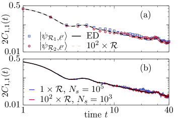
Figure S1: Accuracy of the typicality approach in comparison with exact diagonalization for a 1D Heisenberg chain with $L=16$. (a) Results obtained from two different realizations of ${\cal R}$ show visible fluctuations, while an averaging over $100$ instances of ${\cal R}$ yields results indistinguishable from ED. (b) The averaging over ${\cal R}$ can be combined with the necessary sampling over circuit outputs to reconstruct $C_{1,1}(t)$ in an actual experiment. $N_{s}$ here denotes the number of samples for each individual ${\cal R}$. Even though the total number of runs is the same, the data averaged over $100\times{\cal R}$ agrees better with ED.

.3 Impact of noise on probability distribution

In Fig. 4, we have shown that erroneous gates within ${\cal R}$ turn out to be unimportant for the typicality approach presented in this Letter. However, such errors do have an impact on the probability distribution $P(c_{k})$ which characterizes the state $\ket{\psi_{{\cal R},\ell^{\prime}}}$ Boixo2018S . This is visualized in Fig. S2 where we study the spreading of $\ket{\psi_{{\cal R},\ell^{\prime}}}$ in the computational basis, analogous to Fig. 2 (a). Given the trajectory approach to unravel the quantum channels, $S_{p_{k}}(\ket{\psi_{{\cal R},\ell^{\prime}}})$ is now defined as

$$S_{p_{k}}(\ket{\psi_{{\cal R},\ell^{\prime}}})=\sum_{k=1}^{2^{L}}\rho_{kk}\ln\rho_{kk}\ ,$$ (S9)

where $\rho=(1/N_{{\bf r}})\sum_{{\bf r}}\ket{\psi_{{\cal R},\ell^{\prime}}^{\bf{r}}}\bra{\psi_{{\cal R},\ell^{\prime}}^{\bf{r}}}$ approximates the system’s density matrix. We find that for increasing error rate $p$ (or increasing number of cycles $d$), $S_{p_{k}}(\ket{\psi_{{\cal R},\ell^{\prime}}})$ exhibits a drift from $\ln(2^{L-1})-1+\gamma$ towards $\ln(2^{L-1})$. While the former corresponds to a Gaussian distribution of the $c_{k}$ (i.e., an exponential distribution of $p_{k}=|c_{k}|^{2}$), the latter signals a uniform distribution of the $p_{k}$.

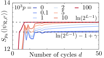
Figure S2: Altering of the output probability distribution of the state $\ket{\psi_{\cal R}}$ due to depolarization errors. For increasing error rate $p$ or increasing number of cycles $d$, $S_{p_{k}}(\ket{\psi_{{\cal R},\ell^{\prime}}})$ drifts from the Gaussian value $\ln(2^{L-1})-1+\gamma$ towards the value $\ln(2^{L}-1)$ which corresponds to a uniform distribution of the $p_{k}$. Data is obtained by averaging over $N_{{\bf r}}=5000$ trajectories for the random circuit shown in Fig. S3.

We note that the averages over quantum trajectories in Figs. 4 and S2 have been obtained for a single realization of the random circuit ${\cal R}$, i.e., a fixed sequence of one-qubit and two-qubit gates with errors being randomly interspersed in each run. This specific realization of ${\cal R}$ is visualized in Fig. S3. Note that due to the additional costs of averaging over trajectories, we have chosen a slightly smaller system with $L=L_{x}\times L_{y}=5\times 4=20$.

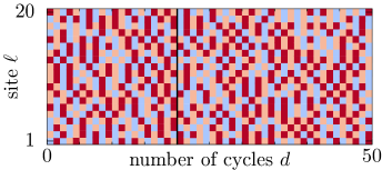
Figure S3: Visualization of the random circuit ${\cal R}$ used to produce the data in Figs. 4 and S2. Different colors signal different one-qubit gates from the set $\{X^{1/2},Y^{1/2},T\}$. The dynamics in Fig. 4 was computed for $d=20$, as indicated by the black vertical line.

.4 Random circuit with CNOT gates

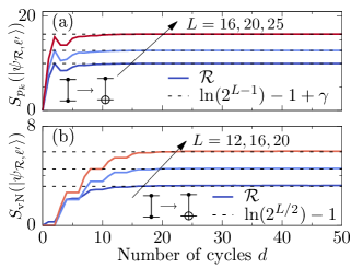
Figure S4: Analogous data as in Fig. 2, but now the two-site gates within ${\cal R}$ are chosen as CNOT gates instead of CZ gates. Once again $S_{p_{k}}(\ket{\psi_{{\cal R},\ell^{\prime}}})$ and $S_{\text{vN}}(\ket{\psi_{{\cal R},\ell^{\prime}}})$ approach their expected values for a random state with increasing cycle number $d$.

In Fig.  2 of the main text, we have shown that the application of the (pseudo-)random circuit ${\cal R}$ yields a state $\ket{\psi_{{\cal R},\ell^{\prime}}}$ which mimics a true Haar-random state, at least with respect to the quantities $S_{p_{k}}$ and $S_{\text{vN}}$. In Fig. S4, we show that the behavior found in Fig. 2 is not caused by ${\cal R}$ being fine-tuned. Specifically, we find that $S_{p_{k}}(\ket{\psi_{{\cal R},\ell^{\prime}}})$ and $S_{\text{vN}}(\ket{\psi_{{\cal R},\ell^{\prime}}})$ quickly approach the expected values for a random state also if the CZ gates are replaced by CNOT gates. Comparing Figs. 2 and S4, however, the convergence seems to be slightly faster in the former case.

.5 Generalization of the typicality relations

Relying on the concept of typicality, we show in this Letter that (pseudo-)random circuits ${\cal R}$ are useful building blocks to study quantum many-body systems. The important realization is that states $\ket{{\cal R}}={\cal R}\ket{0}^{\otimes L}$ generated from such a circuit can faithfully represent the properties of a true Haar-random state $\ket{r}$. In the main text, we have exemplified this approach by considering infinite-temperature spatiotemporal correlation functions $C_{\ell,\ell^{\prime}}(t)$ for one- and two-dimensional quantum spin systems. The overall scheme, however, can be applied in a more general context, which we outline below. (Obviously, instead of spin systems, one could likewise consider fermionic or bosonic models.) One additional application of random circuits would be the preparation of thermal states at finite temperature, which we have already mentioned in the main text. Here, however, we focus on simulations of general correlation functions and of the density of states.

.5.1 Correlation functions

Let $A$ and $B$ denote two hermitian operators and ${\cal D}$ the dimension of the Hilbert space. Then the infinite-temperature correlation function $\langle A(t)B\rangle_{\infty}$ is defined as

$$\langle A(t)B\rangle_{\infty}=\frac{\text{Tr}[A(t)B]}{{\cal D}}\ .$$ (S10)

Without loss of generality, we now assume that $\text{Tr}[A]=\text{Tr}[A(t)]=0$. Then, $\langle A(t)B\rangle_{\infty}$ can be formally rewritten as

$$\frac{\text{Tr}[A(t)B]}{{\cal D}} =\frac{\text{Tr}[A(t)(B+\epsilon)]}{{\cal D}}$$ (S11)

$$=\frac{\text{Tr}[\sqrt{B+\epsilon}A(t)\sqrt{B+\epsilon}]}{{\cal D}}\ ,$$ (S12)

where $\epsilon$ is chosen such that the spectrum of $B+\epsilon$ is non-negative and the square-root operation has to be understood in the eigenbasis of $B$. Exploiting typicality, we can approximate the trace by an expectation value with respect to a random state $\ket{{\cal R}}$ (generated by a random circuit),

$$\langle A(t)B\rangle_{\infty}=\frac{\bra{{\cal R}}\sqrt{B+\epsilon}A(t)\sqrt{B+\epsilon}\ket{{\cal R}}}{\braket{{\cal R}}{{\cal R}}}+{\cal O}(\frac{1}{\sqrt{{\cal D}}})\ ,$$ (S13)

where the statistical error of this approximation vanishes with the inverse square-root of the Hilbert-space dimension. For an interacting system, ${\cal D}$ grows exponentially with the system size. From Eq. (S13), it follows that

$$\langle A(t)B\rangle_{\infty}=c\bra{\widetilde{\cal R}(t)}A\ket{\widetilde{\cal R}(t)}\ ,$$ (S14)

where $\ket{\widetilde{\cal R}}=\sqrt{B+\epsilon}\ket{\cal R}/||\sqrt{B+\epsilon}\ket{\cal R}||$ and $c=||\ket{\widetilde{\cal R}}||^{2}/||\ket{\cal R}||^{2}$. Equation (S14) is a generalization of Eq. (2) from the main text. We note that the construction of the state $\ket{\widetilde{\cal R}}$ can be difficult in practice as the application of the square-root in principle requires the diagonalization of $B$. Assuming that $B$ is a local operator which only acts nontrivially on a few qubits, a full diagonalization can be circumvented however, and an efficient preparation of $\ket{\widetilde{\cal R}}$ might remain possible Richter2019_2S . A significant simplification can be achieved if $B+\epsilon=P$ is a projection, $P=P^{2}$. In this case, no diagonalization is required. Such a scenario applies to the spatiotemporal correlation function $C_{\ell,\ell^{\prime}}(t)$ studied in this Letter. In particular, we have $B=S_{\ell^{\prime}}^{z}$ and $\epsilon=1/2$.

.5.2 Density of states

Here, we briefly outline an algorithm to obtain the density of states (DOS) $\Omega(E)$ of some Hamiltonian ${\cal H}$ on a quantum computer by means of random states, which was first presented in DeRaedt2000S . The DOS is defined as

$$\Omega(E)=\sum_{i}\delta(E-E_{i})=\frac{1}{2\pi}\int_{-\infty}^{\infty}e^{iEt}\text{Tr}[e^{-i{\cal H}t}]\ dt\ ,$$ (S15)

where we have used the definition of the $\delta$ function. Once again, the trace on the right hand side can be approximated as

$$\text{Tr}[e^{-i{\cal H}t}]\approx\bra{\cal R}e^{-i{\cal H}t}\ket{\cal R}=\braket{{\cal R}}{{\cal R}(t)}\ .$$ (S16)

Instead of evolving the state $\ket{{\cal R}(t)}$ in time and projecting the initial state $\ket{\cal R}$ onto it, it is helpful to realize that $\text{Tr}[e^{-i{\cal H}t}]=\text{Tr}[e^{-i{\cal H}t/2}e^{-i{\cal H}t/2}]$. Thus, we can write

$$\text{Tr}[e^{-i{\cal H}t}]\approx\braket{{\cal R}(t/2)}{{\cal R}(t/2)}\ ,$$ (S17)

where the accuracy of the approximation, analogous to Eq. (S13), improves exponentially with the size of the system. The fact that the Fourier transform in Eq. (S15) can be carried out only up to a finite time leads to a broadening of the individual energy peaks. Increasing the time $t$ allows to obtain $\Omega(E)$ with a better and better resolution.

.6 Decomposition of spin-exchange terms into elementary gates

There exist different possibilities to decompose the time-evolution operator $\exp(-ih_{\ell,\ell^{\prime}}t)$ for a two-site Heisenberg Hamiltonian into elementary one- and two-qubit gates. Since two-qubit gates typically have a larger error rate, we here use a representation which only requires three CNOT gates as well as five one-qubit rotations Vatan2004S ; Smith2019S , see Fig. S5 for details. A single step on $L=25$ qubits (i.e., $24$ bond terms) would therefore require $5\times 24=120$ one-qubit and $3\times 24=72$ CNOT gates. Fixing $\delta t=1$, a time evolution up to $t=20$ thus involves $120\times 20=2400$ one-qubit and $72\times 20=1440$ CNOT gates.

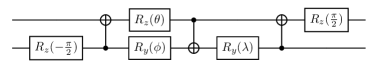
Figure S5: Decomposition of the two-site operator $\exp(-ih_{\ell,\ell^{\prime}}t)$ into elementary one- and two-qubit gates, where $h_{\ell,\ell^{\prime}}=S_{\ell}^{x}S_{\ell^{\prime}}^{x}+S_{\ell}^{y}S_{\ell^{\prime}}^{y}+S_{\ell}^{z}S_{\ell^{\prime}}^{z}$. The decomposition requires three CNOT gates and five one-qubit rotations. The angles of the one-qubit rotations are given by $\theta=\lambda=\pi/2-1/2$ and $\phi=1/2-\pi/2$ Smith2019S .

.7 Dependence of dynamics on depth of ${\cal R}$

In the main text, we have presented numerical results for a fixed depth $d=20$ of the random circuit ${\cal R}$. As exemplified in Fig. 1 (e), this depth turned out sufficient such that the correlation function $C_{1,1}(t)$ obtained from the state $\ket{\psi_{{\cal R},\ell^{\prime}}}$ is indistinguishable from that of a true Haar-random state. In Fig. S6, we now present additional results for shallower random circuits ${\cal R}$ with $d=5,10,15$, for which the resulting state $\ket{\psi_{{\cal R},\ell^{\prime}}}$ is consequently less random. While the data for $d=10$ and $d=15$ agree very well with our previous results for $d=20$, deviations occur for the shallowest circuit with $d=5$. However, even in the latter case, the emerging long-time hydrodynamic tail is very similar to the larger choices of $d$, albeit fluctuations are slightly more pronounced. Thus, even for moderately random states, for which the entanglement entropy differs from the Page value (cf. Fig. 2 from the main text), the resulting dynamics is still a good approximation to the autocorrelation function $C_{1,1}(t)$, and correctly captures the emerging hydrodynamic behavior.

We here leave it to future work to study the dependence of $\bra{\psi_{{\cal R},\ell^{\prime}}(t)}S_{\ell}^{z}\ket{\psi_{{\cal R},\ell^{\prime}}(t)}$ on the depth of ${\cal R}$ in more detail. In particular, it will be an interesting direction to analyze the impact of spatial variations of the randomness of $\ket{\psi_{{\cal R},\ell^{\prime}}}$ on non-local correlations with $\ell\neq\ell^{\prime}$. In this context, it might also be insightful to consider initial conditions where the system is split into patches of Haar-random states, with no initial entanglement between different patches Arute2019S .

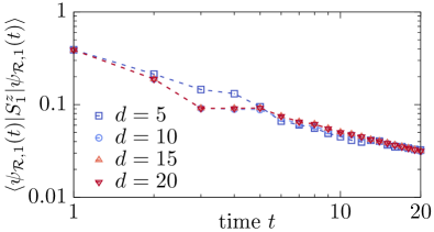
Figure S6: Expectation value $\bra{\psi_{{\cal R},1}(t)}S_{1}^{z}\ket{\psi_{{\cal R},1}(t)}$ for random circuits ${\cal R}$ with different depths $d=5,10,15,20$. Data is analogous to Fig. 1 (e) of the main text. For sufficiently large $d$, the expectation value converges towards the correlation function $2C_{1,1}(t)$. Data is shown for the 1D Heisenberg chain with system size $L=25$. The Trotter time step is fixed to $\delta t=0.5$.

.8 Extraction of diffusion constant for a nonintegrable spin-ladder model

In the main text, we have restricted ourselves to the analysis of the power-law exponents $\alpha(t)$ and $\beta(t)$ which have indicated the emergence of superdiffusive (diffusive) transport in the 1D (2D) Heisenberg model. Let us now demonstrate that our scheme can also quantitatively capture the correct diffusion constant in the case of a nonintegrable model. To this end, we focus on the quasi-1D XY ladder,

$${\cal H} =\sum_{\ell=1}^{L_{x}-1}\sum_{k=1}^{2}\left(S_{\ell,k}^{x}S_{\ell+1,k}^{x}+S_{\ell,k}^{y}S_{\ell+1,k}^{y}\right)$$ (S18)

$$+\sum_{\ell=1}^{L_{x}}\left(S_{\ell,1}^{x}S_{\ell,2}^{x}+S_{\ell,1}^{y}S_{\ell,2}^{y}\right)\ ,$$

where $L_{x}$ denotes the number of rungs. The high-temperature spin diffusion constant of the XY ladder is well-known to be $D\approx 0.95$ Steinigeweg2014S , and the model is a popular example to benchmark numerical methods for transport coefficients Rakovszky2020S .

In Fig. S7, we show numerical data obtained by the approach outlined in the main text. Specifically, we consider a grid of $13\times 2$ qubits, i.e., $26$ qubits in total, and perform a (pseudo)random circuit on the ladder, except for the reference rung $\ell^{\prime}$. We present two examples, namely, $\ell^{\prime}=1$ [edge of the ladder, see Fig. S7 (a)] and $\ell^{\prime}=L_{x}/2$ [center of the ladder, see Fig. S7 (b)]. Subsequently, the resulting state $\ket{\psi_{{\cal R},\ell^{\prime}}}$ is evolved in time with respect to ${\cal H}$ such that correlations spread throughout the system. The time-dependent diffusion coefficient $D(t)$ can then be extracted from the spatial variance $\Sigma^{2}(t)$ of the correlation profile [cf. Eq. (5) in the main text] according to $D(t)=\partial_{t}\Sigma^{2}(t)/2$ ($\ell^{\prime}=L_{x}/2$), or $D(t)=\partial_{t}\Sigma^{2}(t)$ ($\ell^{\prime}=1$, as correlations only spreads in one direction in this case).

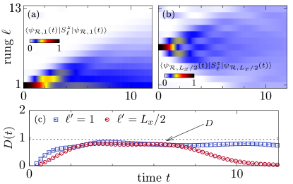
Figure S7: Expectation value $\bra{\psi_{{\cal R},\ell^{\prime}}(t)}S_{\ell}^{z}\ket{\psi_{{\cal R},\ell^{\prime}}(t)}$ for the XY ladder (S18) where the reference rung $\ell^{\prime}$ is chosen as (a) $\ell^{\prime}=1$ or (b) $\ell^{\prime}=L_{x}/2$. (c) Time-dependent diffusion coefficient $D(t)$ extracted from the correlation profiles in (a) and (b). The diffusion constant $D$ is consistent with known results from the literature Rakovszky2020S ; Steinigeweg2014S (horizontal dashed line). Note that the drop of $D(t)$ in the case of $\ell=L_{x}/2$ for $t\gtrsim 8$ indicates the onset of finite-site effects. We have $L_{x}=13$ and $\delta t=0.1$ in all cases.

The resulting data for $D(t)$ is shown in Fig. S7 (c). Above a mean-free time $t\gtrsim 2$, we find that $D(t)$ becomes roughly time-independent, i.e., it becomes a genuine diffusion constant, $D(t)\to D$. In particular, $D$ is almost independent of the choice of $\ell^{\prime}$ in the intermediate time-window $2\lesssim t\lesssim 8$, and is consistent with results from other numerical approaches [dashed line in Fig. S7 (c)] Steinigeweg2014S ; Rakovszky2020S . In this context, let us stress that in some cases it is not advisable to initialize the density peak at the edges of the system, as edge effects might influence the dynamics. For the nonintegrable spin ladder considered here, however, the choices of $\ell^{\prime}=1$ or $\ell^{\prime}=L_{x}/2$ yield consistent results.

Eventually, for $t>8$, we find that $D(t)$ starts to decrease again in the case of $\ell^{\prime}=L_{x}/2$. This can be understood as a finite-size effect as the correlation profile reaches the boundaries of the ladder at these times, cf. Fig. S7 (b). In constrast, finite-size effects are much less pronounced for $\ell^{\prime}=1$, such that $D(t)$ remains constant on longer time scales, which is beneficial for the extraction of $D$.

References

- (1) R. P. Feynman, Int. J. Theor. Phys. 21, 467 (1982).
- (2) U. Schollwöck, Rev. Mod. Phys. 77, 259 (2005); Ann. Phys. 326, 96 (2011).
- (3) A. Weiße, G. Wellein, A. Alvermann, and H. Fehske, Rev. Mod. Phys. 78, 275 (2006).
- (4) F. Verstraete, V. Murg, and J. I. Cirac, Adv. Phys. 57, 143 (2008).
- (5) E. Gull, A. J. Millis, A. I. Lichtenstein, A. N. Rubtsov, M. Troyer, and P. Werner, Rev. Mod. Phys. 83, 349 (2011).
- (6) H. Aoki, N. Tsuji, M. Eckstein, M. Kollar, T. Oka, and P. Werner, Rev. Mod. Phys. 86, 779 (2014).
- (7) G. Carleo and M. Troyer, Science 355, 602 (2017).
- (8) I. Bloch, J. Dalibard, and S. Nascimbène, Nat. Phys. 8, 267 (2012).
- (9) R. Blatt and C. F. Roos, Nat. Phys. 8, 277 (2012).
- (10) I. M. Georgescu, S. Ashhab, and F. Nori, Rev. Mod. Phys. 86, 153 (2014).
- (11) F. Tacchino, A. Chiesa, S. Carretta, D. Gerace, Adv. Quantum Technol. 3, 1900052 (2020).
- (12) A. Kandala, A. Mezzacapo, K. Temme, M. Takita, M. Brink, J. M. Chow, and J. M. Gambetta, Nature 549, 242 (2017).
- (13) P. J. J. O’Malley et al., Phys. Rev. X 6, 031007 (2016).
- (14) A. Chiesa, F. Tacchino, M. Grossi, P. Santini, I. Tavernelli, D. Gerace, and S. Carretta, Nat. Phys. 15, 455 (2019).
- (15) A. Francis, J. K. Freericks, and A. F. Kemper, Phys. Rev. B 101, 014411 (2020).
- (16) K. Choo, C. W. von Keyserlingk, N. Regnault, and T. Neupert, Phys. Rev. Lett. 121, 086808 (2018).
- (17) Y. Wang, Y. Li, Z.-q. Yin and B. Zeng, npj Quantum Inf. 4, 46 (2018).
- (18) A. Smith, B. Jobst, A. G. Green, and F. Pollmann, arXiv:1910.05351.
- (19) H. Lamm and S. Lawrence, Phys. Rev. Lett. 121, 170501 (2018).
- (20) A. Smith, M. S. Kim, F. Pollmann, and J. Knolle, npj Quantum Inf. 5, 106 (2019).
- (21) F. Arute et al., arXiv:2010.07965.
- (22) O. E. Sommer, F. Piazza, and D. J. Luitz, arXiv:2011.08853.
- (23) S. Boixo, S. V. Isakov, V. N. Smelyanskiy, R. Babbush, N. Ding, Z. Jiang, M. J. Bremner, J. M. Martinis, and H. Neven, Nat. Phys. 14, 595 (2018).
- (24) F. Arute et al., Nature 574, 505 (2019).
- (25) J. Preskill, Quantum 2, 79 (2018).
- (26) M. Ippoliti, K. Kechedzhi, R. Moessner, S. L. Sondhi, and V. Khemani, arXiv:2007.11602.
- (27) M. J. Gullans, S. Krastanov, D. A. Huse, L. Jiang, S. T. Flammia, arXiv:2010.09775.
- (28) P. M. Poggi, N. K. Lysne, K. W. Kuper, I. H. Deutsch, and P. S. Jessen, PRX Quantum 1, 020308 (2020).
- (29) B. Bertini, F. Heidrich-Meisner, C. Karrasch, T. Prosen, R. Steinigeweg, and M. Žnidarič, Rev. Mod. Phys. 93, 025003 (2021).
- (30) S. A. Wolf, D. D. Awschalom, R. A. Buhrman, J. M. Daughton, S. von Molnár, M. L. Roukes, A. Y. Chtchelkanova, and D. Treger, Science 294, 1488 (2001).
- (31) L. D’Alessio, Y. Kafri, A. Polkovnikov, and M. Rigol, Adv. Phys. 65, 239 (2016).
- (32) F. Borgonovi, F. M. Izrailev, L. F. Santos, and V. G. Zelevinsky, Phys. Rep. 626, 1 (2016).
- (33) C. Gogolin and J. Eisert, Rep. Prog. Phys. 79, 056001 (2016).
- (34) S. Das Sarma, S. Adam, E. H. Hwang, and E. Rossi, Rev. Mod. Phys. 83, 407 (2011).
- (35) C. Hess, Phys. Rep. 811, 1 (2019).
- (36) A. Scheie, N. E. Sherman, M. Dupont, S. E. Nagler, M. B. Stone, G. E. Granroth, J. E. Moore and D. A. Tennant, Nat. Phys. (2021). https://doi.org/10.1038/s41567-021-01191-6
- (37) S. Hild, T. Fukuhara, P. Schauß, J. Zeiher, M. Knap, E. Demler, I. Bloch, and C. Gross, Phys. Rev. Lett. 113, 147205 (2014).
- (38) N. Jepsen, J. Amato-Grill, I. Dimitrova, W. W. Ho, E. Demler, and W. Ketterle, Nature 588, 403 (2020).
- (39) T. Rakovszky, C. W. von Keyserlingk, and F. Pollmann, arXiv:2004.05177.
- (40) V. Khemani, A. Vishwanath, and D. A. Huse, Phys. Rev. X 8, 031057 (2018).
- (41) H. De Raedt, A. H. Hams, K. Michielsen, S. Miyashita, and K. Saito, Prog. Theor. Phys. Suppl. 138, 489 (2000).
- (42) See Supplemental Material for a derivation of Eq. (2), details on the accuracy and of our approach and generalizations thereof, the impact of noise on the output probability distribution, different circuit designs, the decomposition of spin exchange terms into elementary gates, dynamics for shallower , and the extraction of the diffusion coefficient for a nonintegrable model.
- (43) D. J. Luitz and Y. Bar Lev, Ann. Phys. 529, 1600350 (2017).
- (44) S. Popescu, A. J. Short, and A. Winter, Nat. Phys. 2, 754 (2006).
- (45) S. Goldstein, J. L. Lebowitz, R. Tumulka, and N. Zanghì, Phys. Rev. Lett. 96, 050403 (2006).
- (46) P. Reimann, Phys. Rev. Lett. 99, 160404 (2007).
- (47) S. Lloyd, Ph.D. Thesis, The Rockefeller University (1988), Chapter 3, arXiv:1307.0378.
- (48) J. Gemmer, M. Michel, and G. Mahler, Quantum Thermodynamics (Springer, Berlin, 2004).
- (49) C. Bartsch and J. Gemmer, Phys. Rev. Lett. 102, 110403 (2009).
- (50) T. Heitmann, J. Richter, D. Schubert, and R. Steinigeweg, Z. Naturforsch. A 75, 421 (2020).
- (51) A. Hams and H. De Raedt, Phys. Rev. E 62, 4365 (2000).
- (52) T. Iitaka and T. Ebisuzaki, Phys. Rev. Lett. 90, 047203 (2003).
- (53) G. A. Álvarez, E. P. Danieli, P. R. Levstein, and H. M. Pastawski, Phys. Rev. Lett. 101, 120503 (2008).
- (54) T. A. Elsayed and B. V. Fine, Phys. Rev. Lett. 110, 070404 (2013).
- (55) T. Monnai and A. Sugita, J. Phys. Soc. Jpn. 83, 094001 (2014).
- (56) R. Steinigeweg, J. Gemmer, and W. Brenig, Phys. Rev. Lett. 112, 120601 (2014).
- (57) J. Richter and R. Steinigeweg, Phys. Rev. B 99, 094419 (2019).
- (58) F. Jin, D. Willsch, M. Willsch, H. Lagemann, K. Michielsen, and H. De Raedt, J. Phys. Soc. Jpn. 90, 012001 (2021).
- (59) J. Richter, F. Jin, L. Knipschild, J. Herbrych, H. De Raedt, K. Michielsen, J. Gemmer, and R. Steinigeweg, Phys. Rev. B 99, 144422 (2019).
- (60) B. M. Terhal and D. P. DiVincenzo, Phys. Rev. A 61, 022301 (2000).
- (61) R. Somma, G. Ortiz, J. E. Gubernatis, E. Knill, and R. Laflamme, Phys. Rev. A 65, 042323 (2002).
- (62) J. S. Pedernales, R. Di Candia, I. L. Egusquiza, J. Casanova, and E. Solano, Phys. Rev. Lett. 113, 020505 (2014).
- (63) M. L. Baez, M. Goihl, J. Haferkamp, J. Bermejo-Vega, M. Gluza, and J. Eisert, PNAS 117, 26123 (2020).
- (64) J. Schliemann, A. V. Khaetskii, and D. Loss, Phys. Rev. B 66, 245303 (2002).
- (65) J. Emerson, Y. S. Weinstein, M. Saraceno, S. Lloyd, and D. G. Cory, Science 302, 2098 (2003).
- (66) R. Oliveira, O. C. O. Dahlsten, and M. B. Plenio, Phys. Rev. Lett. 98, 130502 (2007).
- (67) D. Poulin, A. Qarry, R. Somma, and F. Verstraete, Phys. Rev. Lett. 106, 170501 (2011).
- (68) R. Steinigeweg, F. Heidrich-Meisner, J. Gemmer, K. Michielsen, and H. De Raedt, Phys. Rev. B 90, 094417 (2014).
- (69) P. de Vries and H. De Raedt, Phys. Rev. B 47, 7929 (1993).
- (70) F. Vatan and C. Williams, Phys. Rev. A 69, 032315 (2004).
- (71) D. N. Page, Phys. Rev. Lett. 71, 1291 (1993).
- (72) M. Žnidarič, Phys. Rev. A 76, 012318 (2007).
- (73) Y. S. Weinstein, W. G. Brown, and L. Viola, Phys. Rev. A 78, 052332 (2008).
- (74) M. Heyl, P. Hauke, and P. Zoller, Sci. Adv. 5, eaau8342 (2019).
- (75) L. M. Sieberer, T. Olsacher, A. Elben, M. Heyl, P. Hauke, F. Haake, and P. Zoller, npj Quantum Inf. 5, 1 (2019).
- (76) S. Gopalakrishnan, R. Vasseur, and B. Ware, PNAS 116, 16250 (2019).
- (77) M. Ljubotina, M. Žnidarič, and T. Prosen, Nat. Commun. 8, 16117 (2017).
- (78) M. Ljubotina, M. Žnidarič, and T. Prosen, Phys. Rev. Lett. 122, 210602 (2019).
- (79) S. Gopalakrishnan and R. Vasseur, Phys. Rev. Lett. 122, 127202 (2019).
- (80) J. De Nardis, M. Medenjak, C. Karrasch, and E. Ilievski, Phys. Rev. Lett. 123, 186601 (2019).
- (81) F. Weiner, P. Schmitteckert, S. Bera, and F. Evers, Phys. Rev. B 101, 045115 (2020).
- (82) J. Dalibard, Y. Castin, and K. Mølmer, Phys. Rev. Lett. 68, 580 (1992).
- (83) B. Bertini, P. Kos, and T. Prosen, Phys. Rev. X 9, 021033 (2019).
- (84) B. Bertini, P. Kos, and T. Prosen, Phys. Rev. Lett. 123, 210601 (2019).
- (85) P. W. Claeys and A. Lamacraft, Phys. Rev. Lett. 126, 100603 (2021).
- (86) S. Sugiura and A. Shimizu, Phys. Rev. Lett. 111, 010401 (2013).
- (87) M. Motta, C. Sun, A. T. K. Tan, M. J. O’Rourke, E. Ye, A. J. Minnich, F. G. S. L. Brando, and G. K.-L. Chan, Nat. Phys. 16, 205 (2020).
- (88) K. Temme, T. J. Osborne, K. G. Vollbrecht, D. Poulin, and F. Verstraete, Nature 471, 87 (2011).
- (89) J. Cohn, F. Yang, K. Najafi, B. Jones, and J. K. Freericks, Phys. Rev. A 102, 022622 (2020).
- (90) S. Lu, M. C. Bauls, and J. I. Cirac, PRX Quantum 2,020321 (2021).

References

- (1) F. Jin, D. Willsch, M. Willsch, H. Lagemann, K. Michielsen, and H. De Raedt, J. Phys. Soc. Jpn. 90, 012001 (2021).
- (2) J. Richter, F. Jin, L. Knipschild, J. Herbrych, H. De Raedt, K. Michielsen, J. Gemmer, and R. Steinigeweg, Phys. Rev. B 99, 144422 (2019).
- (3) F. Arute et al., Nature 574, 505 (2019).
- (4) S. Boixo, S. V. Isakov, V. N. Smelyanskiy, R. Babbush, N. Ding, Z. Jiang, M. J. Bremner, J. M. Martinis, and H. Neven, Nat. Phys. 14, 595 (2018).
- (5) H. De Raedt, A. H. Hams, K. Michielsen, S. Miyashita, and K. Saito, Prog. Theor. Phys. Suppl. 138, 489 (2000).
- (6) F. Vatan and C. Williams, Phys. Rev. A 69, 032315 (2004).
- (7) A. Smith, M. S. Kim, F. Pollmann, and J. Knolle, npj Quantum Inf. 5, 106 (2019).
- (8) R. Steinigeweg, F. Heidrich-Meisner, J. Gemmer, K. Michielsen, and H. De Raedt, Phys. Rev. B 90, 094417 (2014).
- (9) T. Rakovszky, C. W. von Keyserlingk, and F. Pollmann, arXiv:2004.05177.