A Time-Varying Fine Structure Constant from Naturally Ultralight Dark Matter
Abstract
We present a class of models in which the coupling of the photon to an ultralight scalar field that has a time-dependent vacuum expectation value causes the fine structure constant to oscillate in time. The scalar field is assumed to constitute all or part of the observed dark matter. Its mass is protected against radiative corrections by a discrete exchange symmetry that relates the Standard Model to several copies to itself. The abundance of dark matter is set by the misalignment mechanism. We show that the oscillations in the fine structure constant are large enough to be observed in current and near-future experiments.
I Introduction
With the discovery of the Higgs boson Aad:2012tfa ; Chatrchyan:2012ufa , the Standard Model (SM) of particle physics is now complete. However, cosmological observations tell us that visible matter constitutes only about 20% of the matter in the universe, the remainder being composed of some form of non-luminous dark matter Aghanim:2018eyx . Despite contributing five times more to the energy budget of the universe than visible matter, the basic nature of dark matter has thus far eluded us.
Moduli are among the most well-motivated and compelling dark matter candidates Goldberger:1999uk ; Arvanitaki:2009fg ; Chacko:2012sy ; Coradeschi:2013gda ; Kane:2015jia . They often arise in ultraviolet-complete theories such as string theory, where their vacuum expectation values play a role in determining the values of fundamental parameters such as the fine structure constant. The properties of moduli make them ideal candidates to play the role of dark matter. During inflation, quantum fluctuations are stretched to super horizon length scales, with the result that all scalars lighter than the Hubble scale acquire large random vacuum expectation values. After inflation ends, a light scalar such as a modulus remains frozen away from its minimum by Hubble friction. At late times, the modulus begins to oscillate about its minimum, contributing to the energy density of the universe as a component of dark matter. This framework, termed the misalignment mechanism Linde_1987 , is a natural way of generating an abundance of extremely cold bosonic dark matter from light fields such as moduli.
There has recently been a surge of interest in finding new ways to search for very light dark matter, see e.g. Damour2010_convention ; Damour:2010rm ; Damour:2012rc ; Khmelnitsky:2013lxt ; Stadnik:2014tta ; Arvanitaki:2015iga ; Graham:2015ouw ; Graham:2015ifn ; Stadnik:2015xbn ; Delaunay:2016brc ; Berlin:2016woy ; Geraci:2016fva ; Krnjaic:2017zlz ; Roberts:2017hla ; Arvanitaki:2017nhi ; DeRocco:2018jwe ; Geraci:2018fax ; Irastorza:2018dyq ; Carney:2019cio ; Guo:2019ker ; Grote:2019uvn ; Dev:2020kgz ; Stadnik:2020bfk . One of the the most exciting approaches to finding modulus dark matter is applicable when it is so light that its Compton wavelength is macroscopic, so that the period of its oscillations, set by the inverse of its mass, can be directly observed. As moduli set the value of fundamental constants, they can be searched for by looking for time dependence (”chronovariance”) of these parameters. As a wave of modulus dark matter washes over us, it oscillates with a characteristic time dependence, where is the mass of the modulus field. Therefore a natural way to search for ultralight modulus dark matter is to look for time dependence of the fundamental constants. For early work on time variation of fundamental parameters, see for example Dirac:1937ti ; Chodos:1979vk ; Terazawa:1981ga ; Bekenstein:1982eu ; Marciano:1983wy .
For dark matter to be observable in this way, it must be strongly coupled enough to be detected over noise while oscillating at a low enough frequency that its effects are not averaged away. The condition that the frequency be low translates into the requirement that the mass be small. Since the mass of the modulus receives radiative corrections that depend on the size of its couplings, there is some tension between the condition that the mass remain small and the requirement that the couplings are large enough to be observable, resulting in a naturalness problem.
To understand the naturalness problem, we parametrize the couplings of the modulus to the electromagnetic field in the form,
| (1) |
where is defined as , where is Newton’s constant and is a dimensionless coupling constant that parametrizes the strength of the interaction. For a given mass of the modulus there is a bound on the amplitude of its oscillations, and therefore on the magnitude of the variation of , from the condition that the modulus contribute no more to the energy budget of the universe than the observed dark matter contribution. Current experiments are most sensitive to a modulus mass in the range eV. The corresponding bound on stands at , with the exact value depending on the modulus mass. This coupling in Eq. (1) gives rise to a radiative contribution to the mass of the modulus at two loops 111In the absence of other couplings, the interaction in Eq. (1) can be redefined away. When the electron is present, this redefinition results in a correction to the electron coupling to the photon. In this basis, the natural expectation is that the divergence appears at two-loops.,
| (2) |
where represents an ultraviolet cutoff. As an example, consider a modulus mass of eV for which the bound stands at . For this value of there is a contribution to its mass coming from loops involving the top quark of order eV. Thus, there must be a cancellation in the mass squared of this scalar between the top quark contribution and the bare mass to at least one part in . More generally, for any value of the modulus mass there is an upper bound on above which the conflict comes to the fore. Furthermore, any understanding of the abundance of the modulus requires a consistent ultraviolet completion, since the behavior of a modulus in the early universe is very complicated and is extremely sensitive to the presence of other fields.
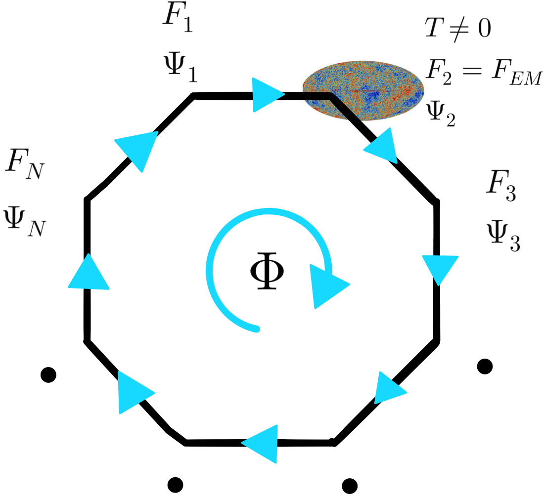
In this paper, we present a framework in which the modulus that controls the fine structure constant can naturally remain ultralight while constituting all of the observed dark matter in the universe. In order to make the modulus naturally light, we employ the mechanism proposed in Ref. Anson1802 . Accordingly, we introduce copies of the SM, where is a number of order a few. If the same modulus controls the fundamental parameters of all the copies of the SM while nonlinearly realizing the symmetry, then the sum of the contributions to the potential of the modulus from each of the copies of the SM cancels to a very high degree of accuracy. The end result is then a modulus with a parametrically smaller mass than naively expected.
A very attractive feature of this framework is that, for certain ranges of the modulus mass and couplings, the misalignment mechanism naturally allows the modulus to constitute all of the observed dark matter. For a given mass and couplings of the modulus, we can determine the thermal corrections to its potential in the early universe. The simplest region of parameter space is that in which the Hubble friction holds the modulus in place and oscillations only begin after thermal effects have become subdominant to the zero temperature potential. Even in this most simple of scenarios, there exists a vast region of parameter space in which the modulus can constitute all of dark matter. In general, finite temperature effects can drastically alter the behavior of the modulus at early times. They can act either to reduce or increase the abundance of dark matter by relaxing the modulus to the minimum or maximum of its potential at high temperatures. Including these effects expands the region of parameter space in which the modulus can play the role of dark matter.
Prospects for probing the time variation of fundamental constants due to ultralight scalars are very promising Arvanitaki2015 ; Arvanitaki:2015iga ; Arvanitaki2018 ; Arvanitaki:2017nhi . In fact, existing data from experiments VanTilburg2015 ; Hess2016 ; Berge2017_MICROSCOPE ; Hoyle1999_EP_CuPb ; Schlamminger2008_EP_BeTi ; Baggio2005_AURIGA ; Kennedy:2020bac ; Vermeulen:2021epa is already sufficient to place constraints on the scenario we propose in the mass range . These limits can be significantly improved in the future by increasing the integration times in the optical-optical clocks and ultimately by taking advantage of the anticipated 229Th nuclear-optical clock Arvanitaki2015 ; nuclearclock . Further advancements can be achieved with the recently proposed earth and space based atomic gravitational wave detectors, which will rely on atom interferometry Arvanitaki2018 ; Coleman_MAGIS100 ; Badurina2019_AION ; Bertoldi2019_AEDGE . The MAGIS and AION experiments Coleman_MAGIS100 ; Badurina2019_AION will be earth based interferometers that are planned to gradually increase in size to finally reach a length of 1 km. MAGIS is currently building a 100 m interferometer Coleman_MAGIS100 , which should be able to probe the proposed model in the mass range. The 1 km stage should increase this range to . Once built, the AION experiment will be able to improve the bounds set by MAGIS at both the 100 m and 1 km scale for the same range of masses . The AEDGE experiment Bertoldi2019_AEDGE is a proposed continuation of the AION experiment that will take advantage of satellites in order to increase the scale of the detector to thousands of kilometers. While it is a very distant prospect, it will have greatly improved sensitivity for masses in the range, .
The outline of this paper is as follows. In Sec. II, we discuss the framework and explain the mechanism that protects the mass of the ultralight modulus. In Sec. III, we study the cosmological history of this class of models and show that the misalignment mechanism can allow the modulus to constitute all of the observed cold dark matter. In Sec. IV we present our results. We determine the current bounds on this class of models and outline the region of parameter space that will be explored by current and future experiments. We conclude in Sec. V
II The Framework
In this section we construct a class of models in which the fine structure constant oscillates in time, and which are free of naturalness problems. We consider a complex scalar that is charged under an approximate U(1) symmetry. This field is assumed to acquire a vacuum expectation value, spontaneously breaking the global symmetry at a scale denoted by . It is convenient to employ an exponential parametrization of ,
| (3) |
Here represents the radial mode in the potential for the scalar field after symmetry breaking, while denotes the pseudo-Nambu-Goldstone boson. We write , where is the vacuum expectation value (VEV) of while represents the fluctuation about this expectation value. The field is assumed to couple to the electromagnetic field strength as shown in Eq. (1). Although this interaction is nonrenormalizable, it can be generated by coupling to some heavy charged fermions that are integrated out. As a consequence of this coupling, changes in the background value of will cause variations in the fine structure constant. However, this coupling violates the U(1) global symmetry explicitly. We therefore expect that, in general, it will generate a potential for , leading to a quadratically divergent mass. Since the parameter controls both the amplitude of the modulation as well as the magnitude of the potential, we require some mechanism that protects the potential against large radiative corrections while still admitting an observable signal. As we now explain, this can be done by employing a discrete symmetry under which the pseudo-Goldstone transforms nonlinearly Anson1802 .
We introduce copies of the SM, each with its own matter content and gauge groups. We label each of these different copies by an index , where runs from 1 to . The copies of the SM are related by a discrete symmetry under which . To each copy of the SM we add a heavy Dirac fermion that carries unit charge under the corresponding hypercharge gauge symmetry, but not under any of the other gauge groups. Each of the fermions is assumed to have a Yukawa coupling to the scalar . Under the symmetry these fields transform as,
| (4) |
The discrete symmetry forces the Yukawa couplings, gauge couplings and masses to be same across all the sectors. The Lagrangian for the is restricted to have the form,
| (5) |
Here the Yukawa coupling can be chosen to be real without loss of generality as any phase of complex can be absorbed into the definition of the complex scalar .
After symmetry breaking, the relevant part of the Lagrangian becomes
| (6) |
where the effective mass of each fermion depends on the VEV of the pseudo-Nambu Goldstone boson
| (7) |
Here the parameter is defined as . After integrating out the fermions we get a contribution at one loop to the effective potential for the pseudo-Nambu Goldstone boson,
| (8) |
where is an ultraviolet cutoff. This integral can be evaluated exactly.
After dropping terms that do not depend on and terms that vanish in the limit , we obtain
| (9) | |||||
where . The first two terms in Eq. (9) are quadratically divergent and logarithmically divergent. However, they can be seen to independent of as long as by virtue of the following identity Anson1802
| (10) |
where is a constant. The finite contribution is, however, -dependent. It can be extracted by expanding the last term in Eq. (9) in the small parameter . To all orders in , we get contributions from each sector that only differ by the phase of the cosine. Due to the identity in Eq. (10), all the terms up to cancel leaving the leading dependence to appear at . These cancellations are a direct consequence of the unbroken symmetry. After performing the integral in (8), the leading -dependent piece arises at order
| (11) |
where is given by
| (12) |
This potential has minima at the locations where runs from 1 to . Integrating out the fermions also leads to an effective coupling of to the gauge kinetic terms of each of the hypercharge gauge fields at low energies,
| (13) |
One of these copies corresponds to the hypercharge gauge boson of the SM. Since the effective potential Eq. (11) is invariant under , we have freedom to shift so that the coupling to SM hypercharge gauge boson simplifies to
| (14) |
Since in our normalization , the coupling to SM photons after spontaneous symmetry breaking takes the same form,
| (15) |
When performs small oscillations about one of the minima of (11), it gives rise to a linear term in the coupling to the photon,
| (16) |
where is the -th minimum of the potential, Eq. (11), and . Comparing to Eq. (1), we see that in terms of the parameters of our model, is given by,
| (17) |
We are now at a stage where we can demonstrate the improvement in naturalness that our model affords. As discussed in the Introduction, the natural expectation is that the mass of scales as
| (18) |
which is just Eq. (2) with the divergence cut off by the mass of the new charged fermion, in this case . To see how our model compares to this, we expand Eq. (11) about the minimum to obtain
The term in brackets represents the improvement with respect to the naive estimate. In order for this expression to be valid, we had assumed that . Because this correction factor is proportional to , we see that as long as is small the mass is parametrically smaller than expected from naive considerations. This demonstrates that our construction can indeed solve the naturalness problem discussed in the Introduction. We note that the mass term for the modulus is generated at one-loop order rather than being given by the naive 2-loop estimate in Eq. (2). This is because both the mass of the modulus and its coupling to the hypercharge gauge boson arise at the same one-loop order when the heavy fermions are integrated out, rather than the mass being generated radiatively from the coupling.
At this stage, the new fermions are electrically charged stable fermions. If the reheat temperature is larger than their mass, then these particles obtain a thermal abundance and will tend to overclose the universe if their masses lie above the TeV scale. In order to avoid this, we allow each of the to decay by introducing a small mixing with the right-handed lepton of the corresponding sector through the interaction
| (20) |
For TeV, we require eV in order to have the particles decay prior to Big Bang nucleosynthesis (BBN) and not pose a cosmological problem.
III Cosmological history
In this section, we will consider the cosmological history of this class of models. We work under the assumption that of the sectors, ours is the only one that is reheated after inflation222One way such a scenario can arise is if there are separate inflatons, one for each sector. Each of the inflatons is assumed to reheat only its own sector. Then the inflaton that slow rolls to its minimum last is associated with the sector that is identified with the SM, while the other sectors are not reheated.. We further assume that is homogenized as a result of inflation. The scalar field evolution is governed by the equation
| (21) |
where the potential is given by
| (22) |
Here is the zero temperature potential given in Eq. (11) while is the contribution to the potential from finite temperature effects. An explicit expression for may be found in Appendix A. At temperatures , the finite temperature contribution to the potential can be approximated as,
| (23) |
Once the temperature falls below its mass, the vector-like fermion begins to exit the bath. Accordingly the form of the thermal contribution to the potential undergoes a change. In the temperature range GeV it is well approximated by the expression,
| (24) |
For , the exponential suppression of the second term in the bracket means that it can be neglected.
The evolution of the scalar field at early times is governed by the extent to which its oscillations are damped by Hubble friction. To keep track of whether the system is underdamped or overdamped at temperature , we define the parameter
| (25) |
where represents the contribution to the mass of the modulus from finite temperature effects,
| (26) |
For the system is overdamped at temperature , while for it is underdamped.
At early times increases as the universe cools down. This can easily be seen from Eq. (23) by noting that when , the mass scales linearly with temperature, , while the Hubble parameter decreases faster, . Eventually, at temperatures of order , the growth of slows down, reaching its maximal value at a temperature . The value of is given by
| (27) |
Here is the reduced Planck mass and is the effective number of degrees of freedom at , consisting of just the SM fields. For , the field oscillates about the minimum of the thermal potential at temperatures of order . The oscillations begin at a temperature such that , given by
| (28) |
Here is the effective number of degrees of freedom at temperatures , which consists of the SM fields and the associated fermion .
Below the temperature , decreases rapidly as the exponential suppression of the second term in Eq. (24) takes effect. Eventually at temperatures , the contribution from the first term in Eq. (24) becomes dominant. In this temperature regime, the mass of the modulus and the Hubble parameter scale identically, . As a result reaches a terminal value , given by
| (29) |
The parameters and play an important role in the description of the system. The value of indicates whether the system undergoes oscillations when , while determines the behavior of the system at temperatures . These parameters are related as
| (30) |
From this relation we can see that in the regime which is always overdamped at early times, , the modulus field is effectively frozen until the temperature-independent part of the potential becomes dominant. In contrast, for the oscillations of the field begin at the temperature and continue till the present time. In the intermediate regime , the field oscillates at temperatures of order . However, these oscillations have ceased by the time the temperature falls below and only resume once the temperature-independent contribution to the potential begins to dominate.
In what follows below we obtain analytic expressions for the contribution of the modulus to the energy density of the universe. We focus on the limiting cases of and , deferring the intermediate range of to our numerical study.
III.1
For the early time evolution is especially simple as Hubble friction freezes the field in place at high temperatures, so that its evolution is independent of . It follows that for sufficiently small the field is effectively fixed until the mass approaches its zero temperature value, . Oscillations begin when , corresponding to a temperature
| (31) |
At this point, we make the standard approximation that transitions instantly from an overdamped harmonic oscillator to an underdamped one. At this stage the potential Eq. (22) is dominated by the zero temperature term,
| (32) | ||||
The mass is constant so the field will oscillate as an underdamped harmonic oscillator around a minimum , with the amplitude decaying as
| (33) |
Since the field is frozen, the value of when can lie anywhere in the range . Therefore can fall into any of the minima of the zero temperature potential, Eq. (32), with equal probability. Consequently the initial misalignment value of the excitation around that minimum can lie anywhere in the range . Due to this randomness in the initial condition and the homogeneity of , it is not possible to determine the exact value of the field today. However, what can be done instead is to average over all possible initial misalignment values, , given that all are equally likely. The expectation value of the energy density can be related to an effective initial amplitude of the field , where . The value of can be obtained by averaging over all values of the initial misalignment, leading to . As a result the expected amplitude of the field today is given by
| (34) |
where represents the current temperature of the Universe. This leads to a final result for the energy density in today,
| (35) |
III.2
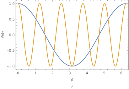
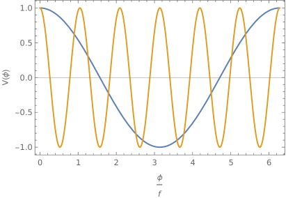
In this subsection, we consider the range of parameter space in which the behaviour of in the early universe at temperatures is like that of a harmonic oscillator that is either underdamped or close to critically damped. When discussing finite temperature effects, it is necessary to distinguish between the cases when is even and is odd. The reason for this can be seen from Fig. 2. In the case of even , the thermal potential pushes towards a maximum of the zero temperature potential. At late times, this results in an increase in the amplitude of oscillations, leading to enhanced abundance of dark matter and a larger signal. For odd , the thermal potential pushes towards a minimum of the zero temperature potential, decreasing the amplitude of oscillations at late times resulting in a suppressed abundance. In this case the situation is even worse because the minimum that is pushed towards is the one in which there is no linear coupling to the photon, so that the signal under consideration is greatly suppressed. Rather than a linear coupling, this minimum leads to a quadratic coupling, which gives rise to different phenomenology Stadnik:2015kia ; Sibiryakov:2020eir that we do not consider here.
odd
In the early universe is driven towards the minimum of the finite temperature potential, . From Fig. 2 we see that the minimum of the finite temperature potential is also a minimum of the zero temperature potential. Consequently the range of values of at the time when oscillations begin, , is significantly smaller than initial .
It follows from this that for each , there is a minimal value of above which this new range covers only the central minimum of the zero temperature potential, . Above this critical value of , which we denote by , always ends up in the central minimum. Furthermore, from Eq. (16) we see that at this central minimum, , the linear coupling of to photons vanishes, resulting in a greatly suppressed signal. The value of can be well approximated by considering evolution only in the regime . The evolution at higher temperatures is less efficient at focusing the range of values of due to the sudden drop of the modulus mass at , which has the effect of regenerating the amplitude of the field. The subsequent evolution of in the regime when and scales with temperature as
| (36) |
It follows that satisfies the condition,
| (37) |
From this we obtain an expression for ,
| (38) |
We see that in the case of odd , for , the field is pushed to the minimum in which does not have the coupling shown in Eq. (1), resulting in a greatly suppressed signal. The abundance of is also suppressed limiting its contribution to dark matter.
even
For even values of the picture is completely different. The minimum of the finite temperature contribution to the potential, which is at , now coincides with the maximum of the zero temperature potential, as can be seen in Fig. 2. Therefore, in the regime the initial value of the modulus at the time when oscillations begin will be close to and the initial amplitude will be very close to
| (39) |
This is very different from the case when the system is overdamped.
The amplitude of the oscillations of today depends on how close the field is to the minimum of the finite temperature potential at the time that the oscillations begin. Given that the mass of the scalar changes as a function of temperature, the simplest way to determine the behavior of at these early times is to employ the conservation of the number density of . The comoving number density of is approximately conserved in the limit that is close enough to a minimum that its potential is quadratic and as long as the WKB approximation holds, . The conserved comoving number density is given by
| (40) |
Based on these considerations the effective initial value of the modulus when the zero temperature potential begins to dominate can be obtained as
| (41) |
We continue to track the evolution of the field after it rolls down to the new minimum, which happens at temperatures of order .
In contrast to the case when , the position of when the zero temperature contribution to the potential begins to dominate is very close to . Since this point corresponds to an extremum of both the finite temperature and zero temperature contributions to the potential, the gradient of the potential at vanishes independent of the temperature. The fact that the potential in the neighborhood of this point is very flat leads to a delayed onset of oscillations Lyth_1992 ; Arvanitaki_anharmonic and interesting phenomenological signatures Arvanitaki:2019rax ; Huang:2020etx . As shown in Appendix B, for the parameters considered in this paper this delay is long enough to ensure that when the oscillations about the new minimum begin, the contributions to the potential from finite temperature effects are already negligible. Therefore, to a good approximation we can assume that the potential has the zero temperature form in Eq. (11) from the time that the oscillations begin.
It is tempting to assume that oscillations about the true minimum occur in a harmonic potential, starting from the temperature , defined in Eq. (31), with an initial amplitude and continuing till today. This leads to the following expression for the contribution of the oscillating field to the energy density today,
| (42) |
However, this expression does not give the correct result for the energy density as it fails to account for the the delay in the time at which the oscillations begin. To include this effect we employ the following empirical approximation Arvanitaki_anharmonic ,
| (43) |
Here
| (44) |
and
| (45) |
The coefficient defined in Eq. (44) corresponds to the correction arising from the delayed onset of oscillations.
The difference between the energy density in Eq. (43) and the naive estimate in Eq. (42) turns out to be quite significant. For TeV the correction factor is for and for .
Since the field is pushed very close to the central maximum of potential, one could imagine that instead of the field homogeneously rolling down to a unique minimum, quantum fluctuations would push the field in some regions of space to the minimum on the other side of the hill, resulting in domain walls. However, just after inflation, quantum fluctuations are given by Lyth_1992 ,
| (46) |
The ratio of fluctuations to the average value of the field is constrained by CMB observations,
| (47) |
Because this quantity changes at most logarithmically between the end of inflation and now Visinelli:2009zm and the emergence of domain walls requires , this scenario does not take place in our model.
IV Signal
In this section, we determine the region of parameter space populated by our model and explore the implications for experiment. Following the conventions employed in Damour2010_convention ; Damour:2010rm ; Arvanitaki2015 , we parametrize the changes to in terms of the variable defined in Eq. (1),
| (48) |
Here represents the amplitude of oscillations of the fine structure constant while denotes the amplitude of oscillations of the scalar field at the location of the earth. We introduce a parameter that represents the fractional contribution of to the total energy density in dark matter,
| (49) |
Experiments place a bound on for a given frequency of oscillation . Then, for a given dark matter fraction , this can be translated into a bound on using Eq. (48).
As can be seen from Eq. (17), the value of is a function of the parameters , , and . From this equation we further see that the value of also depends on the minimum that the field settles in, which is in turn determined by the initial conditions. In our analysis, we take to be the average of available values, e.g. for we have in the regime and in the regime . Additionally for odd values of we ignore the contribution of the central minimum () to the average. This allows us to determine the expected value of consistent with a given set of parameters.
In order to make contact with experiment it is convenient to eliminate the parameter in favor of . The expression for in terms of the other four variables is given in Eq. (32). The parameter space of our model can then be described in terms of the four variables , , and . Using the results of Section III, the expectation value of the dark matter abundance can also be expressed in terms of these parameters, after averaging over the initial conditions for the scalar field . The requirement that, after this averaging, the field constitutes all of the observed dark matter places a restriction on the allowed parameter space and allows us to fix the value of in terms of the three other variables. Then is determined in terms of , and . Taking advantage of the results of Section III, we can obtain semi-analytical expressions for as a function of these three remaining parameters in various regimes. These will prove helpful in illuminating the main features of the detailed numerical results, which we will present later.
IV.1 Analytic Results for
In the overdamped limit, we can use Eqs. (II), (35) and (17) to obtain an expression for in terms of , and ,
| (50) |
Here
| (51) | ||||
and
For convenience, a few values of are given in Table 1. This analytic approximation reproduces our detailed numerical results up to an accuracy of around . From Eq. (50) we can see that decreases as we raise the mass of the fermions . Then, by setting this mass to the lowest value allowed by experiment, we can place an upper bound on as a function of for any given value of .
IV.2 Analytic Results for
| [GeV] | [TeV] | [eV] | ||||
| 10 | 5 | |||||
| 10 | 6 | |||||
| 10 | 10 | |||||
| 10 | 11 |
As increases, the scalar field eventually enters the regime . In this regime, the case of odd is very different from that of even . For odd values of , the region where does not give rise to an observable signal because the field is trapped in the wrong vacuum as discussed in Section III. The boundary of this region is marked by , defined in Eq. (38). The condition translates into a restriction on the allowed range of , and . From Eqs. (II), (29) and (17) we can determine the value of at the boundary of this region to be
| (52) |
where
| (53) | ||||
The numerical values of for a few sample points were given in Table 1. The allowed parameter space is restricted to values of lower than Eq. (52). The line obtained from Eq. (52) is found to reproduce our numerical results up to a factor of 2.
We now turn our attention to the case of even . The expressions for the energy density in the case , Eq. (43), and the case , Eq. (35), differ only by their proportionality constant. It follows from this that scales with and in the same way in both regimes,
| (54) |
where
| (55) | ||||
Here , obtained from Eqs. (35), (II) and (29), corresponds to the mass of the modulus for which and . The numerical values of are given in Table 1 for a few reference points. Equation (54) reproduces the detailed numerical solution up to an accuracy of about .
IV.3 Numerical Results
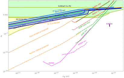
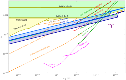
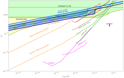
The analytic solutions found in the subsection above are valid in the limiting cases when the scalar field is either highly overdamped or highly underdamped. In order to determine the solution in the region of parameter space where the system transitions between these two regimes, we find it necessary to solve Eq. (21) numerically. We parametrize the model in terms of the four parameters and . As explained earlier, lighter fermion masses are associated with larger values of . In our study we therefore consider two different values of the fermion mass, TeV and TeV, which are close to the current lower bound from collider experiments. In addition, we consider four different values of , the odd values and 11 and the even values and 10. We then scan over for different values of . For each pair, the field was evolved from to starting from 1000 random initial conditions. In the case of odd , we discard any pair such that, for more than of initial conditions, the theory ends up in the vacuum with vanishing signal. For each point we obtain the contribution of to the dark matter density. We also determine the value of , which is obtained by averaging over solutions with , and use this to find the value of at each point from Eqs. (17) and (II).
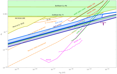
The results of our numerical study are shown in Figs. 3 and 4, where we have plotted as a function of for these theories, along with the current limits and the projected reach of future experiments. Our goal is to identify the region of parameter space that is naturally populated by these models. To this end, for each we have singled out the value of such that, for any larger than this, more than of points will lead to less than the observed abundance of dark matter, . Separately, for each we have singled out the value of such that, for any smaller than this, more than of points will lead to more than the observed abundance of dark matter, . These values have been plotted in Figs. 3 and 4 as the two light blue ( TeV) lines. The region between these lines, which corresponds to the natural parameter space for TeV, has been shaded in. The natural paramater space for TeV has also been shown, shaded in dark blue. We explicitly show the values of the parameters for a few reference points in Table 2.
In order to simplify the numerical computation, the number of effective degrees of freedom in the thermal bath has been held fixed at . The coefficient of the thermal contribution to the potential from the first term in Eq. (24), which also decreases as heavier species go out of the bath, has also been held fixed. These simplifications have an effect on the temperature at which the final oscillations begin, resulting in an overestimate of in the case of the lowest values of by a factor close to two. The error is smaller for larger values of since the oscillations begin earlier, and so there are a greater number of degrees of freedom in the bath at the corresponding .
In Figs. 3 and 4, we have also shown the analytic results obtained in subsections A and B for the case of a fermion mass TeV. For the case of odd , shown in Fig. 3, we have plotted the analytic results obtained from Eqs. (50) and (52), represented by the green and orange lines respectively. We see that there is good agreement between the analytic formulae and our numerical results. For the lightest moduli, the lines are in the overdamped regime and the slope closely follows the one predicted by Eq. (50) (green line). As the mass increases, the line eventually approaches the region where all solutions fall into the central minimum. In this regime the line tracks Eq. (52) (orange line), as expected.
For the plots in Fig. 4 where is even, the behavior for the lowest masses again follows Eq. (50). According to Eq. (50) and Eq. (54), when we should expect that the line jumps while maintaining the same slope. This is exactly what occurs. For larger values of the lower line merges with upper one. This occurs because in the () region, as mentioned earlier, essentially all initial conditions lead to as an initial condition. Therefore the parameter space populated by the model is essentially independent of the initial misalignment angle.
In Figs. 3 and 4, we see the preferred parameter space of our model for various choices of and . From these figures, it is clear that our models span a wide range of and . Larger values of are currently being probed by ongoing experiments while smaller values of are within reach of future experiments. Much as how the QCD axion line provides a goalpost for axion experiments, our small models constitute a well-motivated scenario that future experiments should aim to reach.
V Conclusions
Light moduli are one of the most attractive dark matter candidates. Not only are they ubiquitous in ultraviolet-complete models such as string theory, but the misalignment mechanism provides a simple explanation for their abundance. Despite these appealing features, detecting modulus dark matter remains a challenge. The problem is that the large coupling required to find them tends to be at odds with their very light mass, resulting in a hierarchy problem. In this article, we have shown that a nonlinearly realized symmetry can naturally protect the mass of a modulus against radiative corrections, provided the modulus itself transforms nonlinearly under the . It remains an intriguing open question whether a model that exhibits these features can be constructed within a string theory framework.
Much like the QCD axion, these models have a region of parameter space in which they naturally reproduce the observed dark matter abundance via the misalignment mechanism. The regions of parameter space populated by these models were shown in Figs. 3 and 4 for a few values of . We see from these figures that future experiments searching for chronovariance of the fine structure constant are expected to probe a large part of the preferred parameter space. This class of models is both simple and testable and provides additional theory motivation for exciting new quantum limited experiments.
Acknowledgements
We thank Elizabeth Egbert and Junwu Huang for useful discussions. ZC and AD are supported in part by the National Science Foundation under Grant Number PHY-1914731. ZC is also supported in part by the US-Israeli BSF Grant 2018236. DB and AH are supported in part by the NSF under Grant No. PHY-1914480 and by the Maryland Center for Fundamental Physics (MCFP).
Appendix A Finite Temperature Effects
In this appendix we obtain the contribution to the potential of the modulus from finite temperature effects. For temperatures , the leading contribution arises from the free energy contribution of the vector-like fermion through the dependence of its mass on the value of the modulus, as given in Eq. (7). This contribution is represented by the one-loop diagram shown in Fig. 5.
The form of this contribution is well-known Laine_book ; Kapusta_book and is given by the integral
| (56) |
We can extract the effect on the potential of the modulus by Taylor expanding the potential around and keeping the correction of order ,
| (57) |
This leads to
| (58) |
Another type of contribution arises from the dependence of the free energy of the universe on the hypercharge gauge coupling, which in turn is a function of the VEV of the modulus,
| (59) |
From the above expression we can determine the dependence of this effect on the temperature,
| (60) |
The leading finite temperature contributions to the free energy of the universe that involve the hypercharge gauge coupling arise at two loops. The problem therefore reduces to computing these two loop diagrams. There are three types of diagrams labelled by , and that contribute at this order,
| (61) |
where
| (62) |
The diagrams that give rise to , and are shown in Fig. 6. Here the index runs over all quark and lepton flavors. Using the methods of thermal field theory Laine_book ; Kapusta_book the first diagram, which represents the correction to the free energy from diagrams involving the SM fermions, can be evaluated

as
| (63) | ||||
where we follow the conventions of Laine_book . In these conventions the represent the Euclidean Dirac matrices,
| (64) |
The momenta in the loop integrals are in Euclidean space and have components , where . The symbol refers to integration over the spatial momenta along with summation over the Matsubara frequencies, which are defined as
| (65) |
for fermions and bosons respectively. If the momenta below the symbol appear between curly brackets it corresponds to summation and integration over fermionic boundary conditions while the absence of the brackets indicate bosonic boundary conditions. After the usual Dirac algebra we can express Eq. (63) in terms of known standard integrals Arnold_pureQCD ; Arnold_QCD ,
| (66) | ||||
where . In the limit the last integral vanishes Arnold_QCD . The remaining integrals are well known,
| (67) |
Putting these together we arrive at the result in the high temperature/low mass limit,
| (68) |
where we have expressed in terms of the fine structure constant and the Weinberg angle . Since the represent the hypercharges of the SM fermions and the heavy fermion from our sector, after including all the contributing particles we obtain a factor of .
The second and the third diagrams represent contributions to the free energy from the Higgs doublet. We focus on the high temperature/low mass limit prior to electroweak symmetry breaking. The contribution to the amplitude from the second diagram can be written as the product of the amplitude of two independent one loop diagrams,
| (69) |
In the limit we obtain,
| (70) |
Finally, the third diagram has a form very similar to the first (66), except that now all the integrals are bosonic,
| (71) | ||||
Now, using Eqs. (58) and (61) we put all the pieces together and see that for , the temperature dependent contribution simplifies to,
| (72) |
When the temperature falls below , the contribution given by Eq. (58) becomes exponentially suppressed while the correction to the gauge coupling from Eq. (60) becomes independent of temperature. Additionally, the vector-like fermion of our sector no longer contributes to the Eq. (68), resulting in . Therefore, when the temperature enters the range GeV, the potential takes the form
| (73) |
After electroweak symmetry breaking, we can neglect the contribution from the boson as it is suppressed almost immediately. To get the contribution from photons we multiply the temperature dependent part in Eq. (61) by , which effectively replaces the hypercharge gauge coupling by
| (74) |
Here is a coefficient that changes with the number of species that contribute to the temperature dependent potential. As the universe cools down the number of species that contribute to the potential drops as heavier fields go out of the bath. This in turn, increases the relative strength of Hubble friction. However, this effect is partially compensated for by the rise in the temperature when heavy fields exit the thermal bath.
Therefore, the thermal potential does not change qualitatively until the temperature drops below the mass of the lightest charged particle, the electron, so that . However, in order for this effect to play any role in the evolution of the modulus , the thermal part has to be significant at this point in time, which requires
| (75) |
where was defined in Eq. (38). On the top of that, has to dominate over at . Hence, we have to satisfy
| (76) |
If we additionally require that these conditions overlap with the parameter space not excluded by experiments, we conclude that for no solutions exist that satisfy the above criteria simultaneously. It therefore suffices to consider the high temperature limit of the temperature dependent potential.
Appendix B Form of the Potential at the Onset of Oscillations
In section III we argued that in the case when is even and we are in the underdamped scenario, , the energy density is well approximated by Eq. (43). This formula assumes that field only begins the final stage of oscillations once the finite temperature contributions to the potential are small, so that that the potential is well approximated by its zero temperature form. In order to verify that this condition holds, we will show that for most of the range of parameters considered in Fig. 4, the height difference between the the central maximum and the closest minimum is already within of its final value at the time that the oscillations begin. Recall that the potential is proportional to the sum of two cosines
| (77) | ||||
where is defined in Eq. (26) and is the temperature at which and have quadratic terms of the same magnitude at ,
| (78) |
Naively, oscillations will begin at a temperature when
| (79) |
This equation defines , the effective mass at temperature . Eq. (79) may be rewritten as,
| (80) |
At temperature , Hubble friction is sufficiently small for the field to roll down. However, due to the small gradient near the top of the potential, the moment it reaches the bottom of the potential is delayed by approximately Lyth_1992
| (81) |
where is a measure of how close to the maximum the field is when oscillations about the zero-temperature minimum begin and is the time at which oscillations would start in the overdamped scenario. The value of can be obtained from Eq. (41) as
| (82) |
Before moving on, it is important to point out that the Eq. (81) provides a good qualitative explanation of the evolution, but does not lead to Eq. (43), which is purely empirical. Now, with Eq. (81) we see that the time at which oscillations effectively start is
| (83) |
where is a time when . Using the fact that this transition always occurs during the radiation dominated epoch, when , we can write
| (84) |
Then, with help from Eq. (78) and Eq. (80), we can write
| (85) |
The ratio determines the shape of the potential in Eq. (77) at . Eq. (85) relates this ratio to the parameter . Using these equations we can determine the ratio of the height difference between the central maximum and the closest minimum at relative to the same height difference at zero temperature,
| (86) | ||||
Since the lowest value of for both and is , in order to satisfy we need . This condition is easily fulfilled for as . However, for it is satisfied only for smaller values of the mass of the modulus, eV. Nevertheless, as evident from the numerical simulations presented in Fig. 4, Eq. (54) continues to give a good approximation to the actual result even when this condition is not satisfied.
Appendix C Parametric Resonance
One may worry that decays of into photons may deplete the abundance of dark matter, particularly if the decay rate is enhanced by parametric resonance. In this appendix we consider this question. We find that in the region of parameter space of interest, the condition for parametric resonance is not satisfied. Therefore these decays are slow on cosmological time scales and the abundance of dark matter is not affected.
The Lagrangian for the coupling of to photons can be written as
| (87) |
The resulting equation of motion for the photon is given by
| (88) |
Working in the gauge where this becomes,
| (89) |
This leads to the modified dispersion relation,
| (90) |
Because the plasma mass of the photon is large at the time of the phase transition, we are interested in parametric resonance at times when . Perturbatively expanding the time-dependent dispersion relation, we obtain
| (91) |
When the condensate decays, the resulting photons have the frequency . In phase space, the photons are emitted into a thin shell centered around with width . The occupation number of photons with momentum can be related to the number density of photons as
| (92) |
The integrated Boltzmann equation for the production of photons from the decay of the condensate in the Bose enhanced regime is given by,
| (93) |
where denotes the decay rate of the condensate into photons at zero background photon density. This decay rate can be estimated as
| (94) | |||
For all of the benchmark points in Table 2, the lifetime is greater than years. This is much greater than the age of the universe. Therefore, in the absence of parametric resonance, decays of can safely be neglected.
The parametrically-resonant decay rate can be easily read off from Eq. (93) as
| (95) |
where we have used and . In an expanding universe the proper momentum is redshifting as . This means that the radius of the thin momentum shell is shrinking at the rate of . Since the momentum shell has a finite width , it takes time for an emitted photon to redshift outside the momentum shell. In order to avoid Bose enhancement of decays in the expanding universe, this time scale has to be parametrically smaller than the decay rate at the time of decay,
| (96) |
At early times prior to photon decoupling, the photon has a plasma mass which is larger than . Consequently, decays of into photons are kinematically forbidden until after decoupling. This means that the condition in Eq. (96) only has to be satisfied at times after eV to avoid parametric resonance. Since decoupling happens during matter domination, the Hubble expansion at these times can be related to the field as
| (97) |
where is the fraction of dark matter constituted by . Then, the condition to avoid parametric resonance becomes,
| (98) |
This condition is easily satisfied because the amplitude of the field has already undergone significant damping by the time of recombination.
References
- (1) Georges Aad et al. Observation of a new particle in the search for the Standard Model Higgs boson with the ATLAS detector at the LHC. Phys. Lett. B, 716:1–29, 2012.
- (2) Serguei Chatrchyan et al. Observation of a New Boson at a Mass of 125 GeV with the CMS Experiment at the LHC. Phys. Lett. B, 716:30–61, 2012.
- (3) N. Aghanim et al. Planck 2018 results. VI. Cosmological parameters. 7 2018.
- (4) Walter D. Goldberger and Mark B. Wise. Modulus stabilization with bulk fields. Phys. Rev. Lett., 83:4922–4925, 1999.
- (5) Asimina Arvanitaki, Savas Dimopoulos, Sergei Dubovsky, Nemanja Kaloper, and John March-Russell. String Axiverse. Phys. Rev. D, 81:123530, 2010.
- (6) Zackaria Chacko and Rashmish K. Mishra. Effective Theory of a Light Dilaton. Phys. Rev. D, 87(11):115006, 2013.
- (7) Francesco Coradeschi, Paolo Lodone, Duccio Pappadopulo, Riccardo Rattazzi, and Lorenzo Vitale. A naturally light dilaton. JHEP, 11:057, 2013.
- (8) Gordon Kane, Kuver Sinha, and Scott Watson. Cosmological Moduli and the Post-Inflationary Universe: A Critical Review. Int. J. Mod. Phys. D, 24(08):1530022, 2015.
- (9) Andrei D. Linde. Inflation and Axion Cosmology. Phys. Lett., B201:437–439, 1988.
- (10) Thibault Damour and John F. Donoghue. Equivalence principle violations and couplings of a light dilaton. Phys. Rev. D, 82:084033, Oct 2010.
- (11) Thibault Damour and John F. Donoghue. Phenomenology of the Equivalence Principle with Light Scalars. Class. Quant. Grav., 27:202001, 2010.
- (12) Thibault Damour. Theoretical Aspects of the Equivalence Principle. Class. Quant. Grav., 29:184001, 2012.
- (13) Andrei Khmelnitsky and Valery Rubakov. Pulsar timing signal from ultralight scalar dark matter. JCAP, 02:019, 2014.
- (14) Y.V. Stadnik and V.V. Flambaum. Searching for dark matter and variation of fundamental constants with laser and maser interferometry. Phys. Rev. Lett., 114:161301, 2015.
- (15) Asimina Arvanitaki, Savas Dimopoulos, and Ken Van Tilburg. Sound of Dark Matter: Searching for Light Scalars with Resonant-Mass Detectors. Phys. Rev. Lett., 116(3):031102, 2016.
- (16) Peter W. Graham, Igor G. Irastorza, Steven K. Lamoreaux, Axel Lindner, and Karl A. van Bibber. Experimental Searches for the Axion and Axion-Like Particles. Ann. Rev. Nucl. Part. Sci., 65:485–514, 2015.
- (17) Peter W. Graham, David E. Kaplan, Jeremy Mardon, Surjeet Rajendran, and William A. Terrano. Dark Matter Direct Detection with Accelerometers. Phys. Rev. D, 93(7):075029, 2016.
- (18) Y.V. Stadnik and V.V. Flambaum. Enhanced effects of variation of the fundamental constants in laser interferometers and application to dark matter detection. Phys. Rev. A, 93(6):063630, 2016.
- (19) Cédric Delaunay, Roee Ozeri, Gilad Perez, and Yotam Soreq. Probing Atomic Higgs-like Forces at the Precision Frontier. Phys. Rev. D, 96(9):093001, 2017.
- (20) Asher Berlin. Neutrino Oscillations as a Probe of Light Scalar Dark Matter. Phys. Rev. Lett., 117(23):231801, 2016.
- (21) Andrew A. Geraci and Andrei Derevianko. Sensitivity of atom interferometry to ultralight scalar field dark matter. Phys. Rev. Lett., 117(26):261301, 2016.
- (22) Gordan Krnjaic, Pedro A.N. Machado, and Lina Necib. Distorted neutrino oscillations from time varying cosmic fields. Phys. Rev. D, 97(7):075017, 2018.
- (23) Benjamin M. Roberts, Geoffrey Blewitt, Conner Dailey, Mac Murphy, Maxim Pospelov, Alex Rollings, Jeff Sherman, Wyatt Williams, and Andrei Derevianko. Search for domain wall dark matter with atomic clocks on board global positioning system satellites. Nature Commun., 8(1):1195, 2017.
- (24) Asimina Arvanitaki, Savas Dimopoulos, and Ken Van Tilburg. Resonant absorption of bosonic dark matter in molecules. Phys. Rev. X, 8(4):041001, 2018.
- (25) William DeRocco and Anson Hook. Axion interferometry. Phys. Rev. D, 98(3):035021, 2018.
- (26) Andrew A. Geraci, Colin Bradley, Dongfeng Gao, Jonathan Weinstein, and Andrei Derevianko. Searching for Ultralight Dark Matter with Optical Cavities. Phys. Rev. Lett., 123(3):031304, 2019.
- (27) Igor G. Irastorza and Javier Redondo. New experimental approaches in the search for axion-like particles. Prog. Part. Nucl. Phys., 102:89–159, 2018.
- (28) Daniel Carney, Anson Hook, Zhen Liu, Jacob M. Taylor, and Yue Zhao. Ultralight Dark Matter Detection with Mechanical Quantum Sensors. 8 2019.
- (29) Huai-Ke Guo, Keith Riles, Feng-Wei Yang, and Yue Zhao. Searching for Dark Photon Dark Matter in LIGO O1 Data. Commun. Phys., 2:155, 2019.
- (30) H. Grote and Y.V. Stadnik. Novel signatures of dark matter in laser-interferometric gravitational-wave detectors. Phys. Rev. Res., 1(3):033187, 2019.
- (31) Abhish Dev, Pedro A.N. Machado, and Pablo Martínez-Miravé. Signatures of Ultralight Dark Matter in Neutrino Oscillation Experiments. 7 2020.
- (32) Yevgeny V. Stadnik. New bounds on macroscopic scalar-field topological defects from non-transient signatures due to environmental dependence and spatial variations of the fundamental constants. Phys. Rev. D, 102:115016, 2020.
- (33) Paul A. M. Dirac. The Cosmological constants. Nature, 139:323, 1937.
- (34) Alan Chodos and Steven L. Detweiler. Where Has the Fifth-Dimension Gone? Phys. Rev. D, 21:2167, 1980.
- (35) Hidezumi Terazawa. Cosmological Origin of Mass Scales. Phys. Lett. B, 101:43–47, 1981.
- (36) J. D. Bekenstein. Fine Structure Constant: Is It Really a Constant? Phys. Rev. D, 25:1527–1539, 1982.
- (37) William J. Marciano. Time Variation of the Fundamental ’Constants’ and Kaluza-Klein Theories. Phys. Rev. Lett., 52:489, 1984.
- (38) Anson Hook. Solving the hierarchy problem discretely. Phys. Rev. Lett., 120:261802, Jun 2018.
- (39) Asimina Arvanitaki, Junwu Huang, and Ken Van Tilburg. Searching for dilaton dark matter with atomic clocks. Phys. Rev. D, 91:015015, Jan 2015.
- (40) Asimina Arvanitaki, Peter W. Graham, Jason M. Hogan, Surjeet Rajendran, and Ken Van Tilburg. Search for light scalar dark matter with atomic gravitational wave detectors. Phys. Rev. D, 97:075020, Apr 2018.
- (41) Ken Van Tilburg, Nathan Leefer, Lykourgos Bougas, and Dmitry Budker. Search for ultralight scalar dark matter with atomic spectroscopy. Phys. Rev. Lett., 115:011802, Jun 2015.
- (42) A. Hees, J. Guéna, M. Abgrall, S. Bize, and P. Wolf. Searching for an oscillating massive scalar field as a dark matter candidate using atomic hyperfine frequency comparisons. Phys. Rev. Lett., 117:061301, Aug 2016.
- (43) Joel Bergé, Philippe Brax, Gilles Métris, Martin Pernot-Borràs, Pierre Touboul, and Jean-Philippe Uzan. MICROSCOPE Mission: First Constraints on the Violation of the Weak Equivalence Principle by a Light Scalar Dilaton. Phys. Rev. Lett., 120(14):141101, 2018.
- (44) G. L. Smith, C. D. Hoyle, J. H. Gundlach, E. G. Adelberger, B. R. Heckel, and H. E. Swanson. Short-range tests of the equivalence principle. Phys. Rev. D, 61:022001, Dec 1999.
- (45) S. Schlamminger, K.-Y. Choi, T. A. Wagner, J. H. Gundlach, and E. G. Adelberger. Test of the equivalence principle using a rotating torsion balance. Phys. Rev. Lett., 100:041101, Jan 2008.
- (46) L. Baggio, M. Bignotto, M. Bonaldi, M. Cerdonio, L. Conti, P. Falferi, N. Liguori, A. Marin, R. Mezzena, A. Ortolan, S. Poggi, G. A. Prodi, F. Salemi, G. Soranzo, L. Taffarello, G. Vedovato, A. Vinante, S. Vitale, and J. P. Zendri. 3-mode detection for widening the bandwidth of resonant gravitational wave detectors. Phys. Rev. Lett., 94:241101, Jun 2005.
- (47) Colin J. Kennedy, Eric Oelker, John M. Robinson, Tobias Bothwell, Dhruv Kedar, William R. Milner, G. Edward Marti, Andrei Derevianko, and Jun Ye. Precision Metrology Meets Cosmology: Improved Constraints on Ultralight Dark Matter from Atom-Cavity Frequency Comparisons. Phys. Rev. Lett., 125(20):201302, 2020.
- (48) Sander M. Vermeulen et al. Direct limits for scalar field dark matter from a gravitational-wave detector. 3 2021.
- (49) P G Thirolf, B Seiferle, and L von der Wense. The 229-thorium isomer: doorway to the road from the atomic clock to the nuclear clock. Journal of Physics B: Atomic, Molecular and Optical Physics, 52(20):203001, sep 2019.
- (50) Jon Coleman. Matter-wave Atomic Gradiometer InterferometricSensor (MAGIS-100) at Fermilab. PoS, ICHEP2018:021, 2019.
- (51) L. Badurina et al. AION: An Atom Interferometer Observatory and Network. 2019.
- (52) Yousef Abou El-Neaj et al. AEDGE: Atomic Experiment for Dark Matter and Gravity Exploration in Space. 2019.
- (53) Y.V. Stadnik and V.V. Flambaum. Can dark matter induce cosmological evolution of the fundamental constants of Nature? Phys. Rev. Lett., 115(20):201301, 2015.
- (54) Sergey Sibiryakov, Philip Sorensen, and Tien-Tien Yu. BBN constraints on universally-coupled ultralight scalar dark matter. 6 2020.
- (55) D. H. Lyth. Axions and inflation: Vacuum fluctuations. Phys. Rev. D, 45:3394–3404, May 1992.
- (56) Asimina Arvanitaki, Savas Dimopoulos, Marios Galanis, Luis Lehner, Jedidiah O. Thompson, and Ken Van Tilburg. Large-misalignment mechanism for the formation of compact axion structures: Signatures from the QCD axion to fuzzy dark matter. Phys. Rev. D, 101(8):083014, 2020.
- (57) Asimina Arvanitaki, Savas Dimopoulos, Marios Galanis, Luis Lehner, Jedidiah O. Thompson, and Ken Van Tilburg. Large-misalignment mechanism for the formation of compact axion structures: Signatures from the QCD axion to fuzzy dark matter. Phys. Rev. D, 101(8):083014, 2020.
- (58) Junwu Huang, Amalia Madden, Davide Racco, and Mario Reig. Maximal axion misalignment from a minimal model. 6 2020.
- (59) Luca Visinelli and Paolo Gondolo. Dark Matter Axions Revisited. Phys. Rev. D, 80:035024, 2009.
- (60) Mikko Laine and Aleksi Vuorinen. Basics of Thermal Field Theory, volume 925. Springer, 2016.
- (61) J.I. Kapusta and Charles Gale. Finite-temperature field theory: Principles and applications. Cambridge Monographs on Mathematical Physics. Cambridge University Press, 2011.
- (62) Peter Arnold and Chengxing Zhai. Three-loop free energy for pure gauge qcd. Phys. Rev. D, 50:7603–7623, Dec 1994.
- (63) Peter Arnold and Chengxing Zhai. Three-loop free energy for high-temperature qed and qcd with fermions. Phys. Rev. D, 51:1906–1918, Feb 1995.