Batch Group Normalization

Abstract

Deep Convolutional Neural Networks (DCNNs) are hard and time-consuming to train. Normalization is one of the effective solutions. Among previous normalization methods, Batch Normalization (BN) performs well at medium and large batch sizes and is with good generalizability to multiple vision tasks, while its performance degrades significantly at small batch sizes. In this paper, we find that BN saturates at extreme large batch sizes, i.e., 128 images per worker, as well and propose that the degradation/saturation of BN at small/extreme large batch sizes is caused by noisy/confused statistic calculation. Hence without adding new trainable parameters, using multiple-layer or multi-iteration information, or introducing extra computation, Batch Group Normalization (BGN) is proposed to solve the noisy/confused statistic calculation of BN at small/extreme large batch sizes with introducing the channel, height and width dimension to compensate. The group technique in Group Normalization (GN) is used and a hyper-parameter $\rm G$ is used to control the number of feature instances used for statistic calulation, hence to offer neither noisy nor confused statistic for different batch sizes. We empirically demonstrate that BGN consistently outperforms BN, Instance Normalization (IN), Layer Normalization (LN), GN, and Positional Normalization (PN), across a wide spectrum of vision tasks, including image classification, Neural Architecture Search (NAS), adversarial learning, Few Shot Learning (FSL) and Unsupervised Domain Adaptation (UDA), indicating its good performance, robust stability to batch size and wide generalizability. For example, for training ResNet-50 on ImageNet with a batch size of 2, BN achieves Top1 accuracy of $66.512\%$ while BGN achieves $76.096\%$ with notable improvement.

Introduction

Since AlexNet was proposed in (Krizhevsky, Sutskever, and Hinton 2012), Deep Convolutional Neural Network (DCNN) has been a popular method for vision tasks including image classification (Deng et al. 2009), object detection (Lin et al. 2014) and semantic segmentation (Everingham et al. ). DCNNs are usually composed of convolutional layers, normalization layers, activation layers, etc. Normalization layers are important in improving performance and speeding up training.

Batch Normalization (BN) was one of the early proposed normalization methods (Ioffe and Szegedy 2015) and is widely used. It normalizes the feature map with the mean and variance calculated along with the batch, height, and width dimension of a feature map and then re-scales and re-shifts the normalized feature map to ensure DCNN representation ability. Based on BN, many normalization methods for other tasks have been proposed. For example, Layer Normalization (LN) was proposed for calculating the statistics along the channel, height and width dimension for Recurrent Neural Network (RNN) (Ba, Kiros, and Hinton 2016). Weight Normalization (WN) was proposed to parameterize the weight vector for supervised image recognition, generative modelling, and deep reinforcement learning (Salimans and Kingma 2016). Divisive Normalization which includes BN and LN as special cases was proposed for image classification, language modeling and super-resolution (Ren et al. 2016). Instance Normalization (IN) where the statistics were calculated from the height and width dimension was proposed for fast stylization (Ulyanov, Vedaldi, and Lempitsky 2016). Instead of calculating the statistics from data, Normalization Propagation estimated them data-independently from the distribution in layers (Arpit et al. 2016). Group Normalization divided the channels into groups and calculated the statistics for each grouped channel, height and width dimension, showing stability to batch sizes (Wu and He 2018). Positional Normalization (PN) was proposed to calculate the statistics along the channel dimension for generative networks (Li et al. 2019a).

Among these normalization methods, BN can usually achieve good performance at medium and large batch sizes. However, its performance degrades at small batch sizes, as shown in pre works (Wu and He 2018; Ioffe 2017). Furthermore, as shown in our experiments, BN’s performance saturates at extreme large batch sizes, i.e., 128 images per worker. GN enjoys a greater degree of stability at different batch sizes, while slightly under-performs BN at medium and large batch sizes. Other normalization methods, including IN, LN and PN perform well in specific tasks, but are usually less generalizable to and under-perform in other vision tasks. As reviewed in Related Work, many works have been conducted on proposing new normalization methods with good performance, stability and generalizability.

In this paper, unlike those reviewed works where additional trainable parameters, extra computation or additional information are used, Batch Group Normalization (BGN) is parameter- and computation-efficient. We know the fact that mini-batch training usually can perform better than single-batch (use a single image example as the DCNN input per iteration) and all-batch training (use all image examples as the DCNN input per iteration), as single-batch training can indicate noisy gradient while all-batch training may not indicate representative gradient (each image example indicates gradient with different directions, thus, adding them all indicates confused gradient). Inspired by this fact, we think the number of feature instances in statistic calculation in normalization should also be moderate, i.e., the degraded/saturated performance of BN on small/extreme large batch sizes is due to noisy/confused statistic calculation.

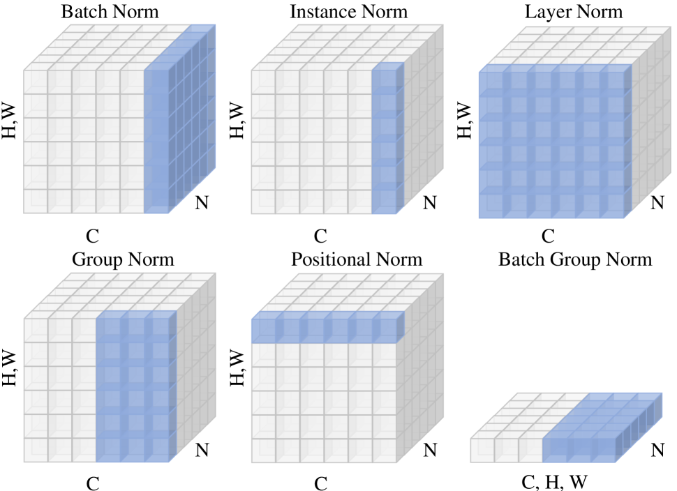
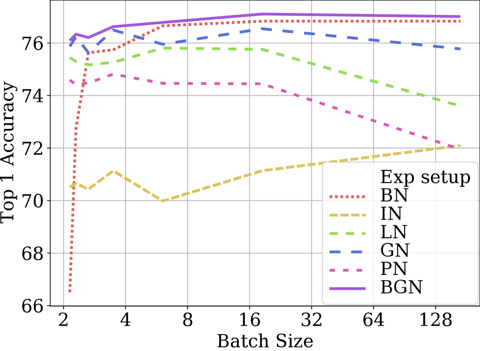
Figure 1: top). The difference between the statistic calculation in BN, IN, LN, GN, PN and BGN. Each subplot shows a feature map tensor, with N, C and (H, W) as the batch, channel and spatial axes. The pixels in blue are used to compute the statistics. This figure is inspired by (Wu and He 2018). bottom). The Top1 accuracy of training ResNet-50 on ImageNet, with different batch sizes, and with BN, IN, LN, GN, PN and BGN as the normalization.

Hence, BGN is proposed to facilitate the performance degradation/saturation of BN at small/extreme large batch sizes with the group technique from GN. It merges the channel, height and width dimensions into a new dimension, divides the new dimension into feature groups, and calculates the statistics across the whole mini-batch and feature group. A hyper-parameter $\rm G$ is used to control the level of feature division and to supply proper statistics for different batch sizes. The difference between BN, IN, LN, GN, PN and BGN, with respect to the dimensions along which the statistics are computed, are illustrated in Fig. 1(top). The Top1 accuracy of training ResNet-50 on ImageNet by using BN, IN, LN, GN, PN and BGN as the normalization layer are shown in Fig. 1(bottom). Without adding trainable parameters, using extra information or requiring extra computation, BGN achieves both good performance and stability at different batch sizes. We test on Neural Architecture Search (NAS), adversarial learning, Few Show Learning (FSL) and Unsupervised Domain Adaptation (UDA), BGN outperforms BN, IN, LN, GN and PN, showing its good generalizability.

Related Work

Why normalization works? The effectiveness of BN has been attributed to internal covariate shift where the distribution of each layer’s input changes and hence lower learning rate and careful parameter initialization are essential to guarantee good training in DCNNs without normalization (Ioffe and Szegedy 2015). Other works have investigated the reasons for the success of normalization. For example, Santurkar et al. (Santurkar et al. 2018) proposed that the effectiveness of BN has little to do with internal covariate shift, but to make the optimization landscape smoother and hence to introduce stable gradients and faster training. Bjorck et al. (Bjorck et al. 2018) proposed that allowing larger learning rates is the main reason for BN to achieve faster convergence and better generalization. A theoretical support was supplied for the effectiveness of BN in tuning learning rates less (Arora, Lyu, and Li 2019). Luo et al. demonstrated that BN and regularization share the same traits (Luo et al. 2019b). A quantitative analysis was provided to compare the gradient descent with and without BN on Ordinary Least Squares (OLS) (Cai, Li, and Shen 2019). In (Fan 2017), it was shown with fuzzy neural networks that BN estimates the correct bias induced by the generalized hamming distance. In contrast, BN was proved to be the cause of the gradient explosion for DCNNs without residual learning (Yang et al. 2019). In (Li et al. 2019b), from the theoretical and statistical aspects, the disharmony between dropout and BN was explained. It was claimed that BN is not unique for stable training, higher learning rates, accelerated convergence and improved generalization, and can be replaced by better initialization (Zhang, Dauphin, and Ma 2019; De and Smith 2020). Normalization layers were shown to introduce a stable gradient magnitude when training the Long-Short-Term Memory (LSTM) (Hou et al. 2019). Even though many interesting theories have been proposed to explain the effectiveness of BN, there is still a lack of consensus.

Improvements Previous works can be further improved. Centered WN proposed to add a learnable parameter to adjust the weight norm in WN (Huang et al. 2017). Recurrent BN was proposed to not only apply BN in the input-to-hidden, but also to the hidden-to-hidden transformation of RNNs (Cooijmans et al. 2016). Batch Renormalization was proposed to decrease the dependence of BN on the size of mini-batches (Ioffe 2017). Riemannian approach was combined to BN on the space of weight vectors, which improves BN’s performance on various DCNN architectures and datasets (Cho and Lee 2017). EvalNorm was proposed to estimate the corrected normalization statistics during evaluation to address the performance degradation of BN (Singh and Shrivastava 2019). Moving Average BN proposed using the batch statistics in the backward propagation of traditional BN (Yan et al. 2019). Based on LN, Adaptive Normalization proposed to modify bias and gain by using a new transformation function (Xu et al. 2019a). Root Mean Square LN proposed to abandon the re-centering and keep the re-scaling in LN (Zhang and Sennrich 2019).

Researchers are also looking into non-linear normalizing techniques with extra computation. For example, ZCA was used to replace the centering and scaling calculations in BN, resulting in Decorrelated BN (Huang et al. 2018). Iterative Normalization proposed using Newton iterations to avoid the eigen-decomposition in Decorrelated BN, indicating much more efficient whitening (Huang et al. 2019). Instead of normalizing in the spatial space, Spectral Normalization was proposed to normalize the spectral norm of weights and was used in Generative Adversarial Networks (GANs) (Miyato et al. 2018) and adversarial training (Farnia, Zhang, and Tse 2019).

Learning-to-normalize is also explored. Different normalization methods introduced before can be combined to achieve better performance and generalization. Batch-Instance Normalization (BIN) was proposed for adaptively style-invariant neural networks, with using a trainable parameter to combine the feature maps calculated from BN and IN (Nam and Kim 2018). Switchable Normalization (SN) was proposed by using trainable parameters on the mean and variance calculated in BN, IN and LN to learn new statistics (Luo et al. 2019a, c). Sparse SN used SparseMax to make the trainable parameters in SN sparse (Shao et al. 2019). In Instance-Level Meta Normalization (Jia, Chen, and Chen 2019), feature feed-forward and gradient back-propagation were used to learn the normalization parameters.

Others Normalization can be used as a method to achieve a task directly. For example, a real-time and arbitrary style transfer was achieved by aligning the mean and variance of the content features to that of the style features (Huang and Belongie 2017). Domain adaptation was achieved by changing the statistics from the source domain to the target domain (Li et al. 2018b). New tasks can be solved by using BN to combine learned tasks (Data et al. 2018). Specific normalization methods have also been specifically proposed for cross-domain tasks (Li and Vasconcelos 2019; Wang et al. 2019), global covariance pooling networks (Li et al. 2018a), multitask learning (Chen et al. 2018; Deecke, Murray, and Bilen 2019), UDA (Chang et al. 2019), semantic image synthesis (Park et al. 2019), medical area (Zhou and Yang 2019; Zhou et al. 2019; Zhou 2019), and scene text detection (Xu et al. 2019b). Kalman Normalization (KN) was proposed to combine internal representations across multiple DCNN layers (Wang et al. 2018). And, instead of using $L^{2}$ norm, $L^{1}$ and $L^{\infty}$ norm were proposed for numerical stability in low-precision calculation (Hoffer et al. 2018).

Methodology

In a DCNN with $\rm L$ layers, for an input feature map $\mathcal{F}^{l},l\in[1,\rm L]$, which is usually with four dimensions $(\rm N,C,H,W)$, where $\rm N,C,H,W$ is the batch, channel, height and width dimension respectively. For simplification, $n\in\rm[1,N],c\in\rm[1,C],h\in\rm[1,H],w\in\rm[1,W]$ are the corresponding batch, channel, height and width indices and will not be repeatly defined in the following usage. The feature map at $(l+1)$th layer is calculated as:

$$\mathcal{F}^{l+1}=\psi(\theta(\phi(\mathcal{F}^{l},w^{l},b^{l}),\gamma^{l},\beta^{l}))$$ (1)

where $w^{l}$ and $b^{l}$ are the trainable weight and bias parameters in convolutional layers, $\gamma^{l}$ and $\beta^{l}$ are the trainable re-scale and re-shift parameters in normalization layers, $\psi(\cdot)$ is the activation function. $\theta(\cdot)$ is the normalization function. $\phi(\cdot)$ is the convolusion function.

A typical normalization layer includes four steps: (1) divide the feature map into feature groups; (2) calculate the $mean$ and $variance$ statistics for each feature group; (3) normalize each feature group with the calculated statistics; (4) re-scale and re-shift the normalized feature map to maintain the DCNN representation ability. For example, in BN, the feature map is divided along the channel dimension, the $mean$ $\mu_{c}$ and $variance$ $\delta_{c}^{2}$ are calculated along the batch, height and width dimension as:

$$\mu_{c}=\frac{1}{\rm N\times\rm H\times\rm W}\sum\limits_{n=1}^{\rm N}\sum\limits_{h=1}^{\rm H}\sum\limits_{w=1}^{\rm W}f_{n,c,h,w}$$ (2)

$$\delta_{c}^{2}=\frac{1}{\rm N\times\rm H\times\rm W}\sum\limits_{n=1}^{\rm N}\sum\limits_{h=1}^{\rm H}\sum\limits_{w=1}^{\rm W}(f_{n,c,h,w}-\mu_{c})^{2}$$ (3)

Then the feature map is normalized as:

$$\hat{f}_{n,c,h,w}=\frac{f_{n,c,h,w}-\mu_{c}}{\sqrt{\delta_{c}^{2}+\epsilon}}$$ (4)

$\epsilon$ is a small number added for division stability. In order to maintain the DCNN representation ability, extra trainable parameters are added for each feature channel:

$$f^{\prime}_{n,c,h,w}=\gamma_{c}\hat{f}_{n,c,h,w}+\beta_{c}$$ (5)

Table 1: The Top1 validation accuracy of BGN on ImageNet with ResNet-50. G is set to be from 512 to 1.

Batch size	Group number
	512	256	128	64	32	16	8	4	2	1
128	77.008	75.936	76.256	76.096	75.984	75.504	76.016	75.632	75.520	75.360
2	63.968	66.000	68.160	70.064	71.856	72.832	74.928	75.120	75.968	76.096

By including multiple examples into statistic calculation, BN enjoys good performance at medium and large batch sizes and good generalizability to multiple vision tasks, i.e. NAS. However, its performance degrades dramatically, i.e., $>10\%$ in our ImageNet experiment, at small batch sizes. In order to improve this shortage, GN includes grouped channel dimension into statistic calculation:

$$\mu_{n,g}=\frac{1}{\rm M\times\rm H\times\rm W}\sum\limits_{m=(g-1)\cdot\rm M+1}^{\rm g\cdot M}\sum\limits_{h=1}^{\rm H}\sum\limits_{w=1}^{\rm W}f_{n,m,h,w}$$ (6)

$$\delta_{n,g}^{2}=\frac{1}{\rm M\times\rm H\times\rm W}\sum\limits_{m=(g-1)\cdot\rm M+1}^{\rm g\cdot M}\sum\limits_{h=1}^{\rm H}\sum\limits_{w=1}^{\rm W}(f_{n,m,h,w}-\mu_{n,g})^{2}$$ (7)

where $g\in\rm[1,G]$, $\rm G$ is a hyper parameter - group number, $\rm M=C//G$, $//$ is floor division. GN enjoys good stability to different batch sizes, however, its performance is slightly lower than BN at medium and large batch sizes and its generalizability to other vision tasks is weaker than BN. Except these known phenomena, our experiments show that BN saturates at extreme large batch sizes.

We think the degradation/saturation of BN at small/extreme large batch sizes are caused by noisy/confused statistic calculation. Similar indication also exists in mini-batch training, where single-batch/all-batch training are usually worse than mini-batch training, as noisy/confused gradients are calculated. To facilitate this, we propose BGN where the number of feature instances used for statistic calculation is controlled to be proper by using the group technique in GN. To be in more details, we first merge the channel, height and width dimensions into a new dimension and achieve $\rm\mathcal{F}^{l}_{N\times D}$, where $\rm D=C\times H\times W$. The mean $\mu_{g}$ and variance $\delta_{g}^{2}$ are calculated along the batch and new dimension as:

$$\mu_{g}=\frac{1}{\rm N\times\rm S}\sum\limits_{n=1}^{\rm N}\sum\limits_{d=(g-1)\cdot\rm S+1}^{\rm g\cdot S}f_{n,d}$$ (8)

$$\delta_{g}^{2}=\frac{1}{\rm N\times\rm S}\sum\limits_{n=1}^{\rm N}\sum\limits_{d=(g-1)\cdot\rm S+1}^{\rm g\cdot S}(f_{n,d}-\mu_{g})^{2}$$ (9)

where $\rm G$ is the number of groups that the new dimension is divided and is a hyper-parameter, $\rm S=M/G$ is the number of instances inside each divided feature group. When the batch size is small, a small G is used to combine the whole new dimension into statistic calculation to avoid noisy statistics, while when the batch size is large, a large G is used to split the new dimension into small pieces for calculating the statistics to avoid confused statistics. $\gamma_{c}$ and $\beta_{c}$ are used in the same way as BN. In BN, $\mu_{c}$ and $\delta_{c}^{2}$ used in the test are the moving average of that in the training stage. The proposed BGN uses this policy as well.

Relation to General Batch Group Normalization (GBGN) GBGN (Summers and Dinneen 2019) could be confused as a similar work to BGN, we clarify our contributions as below: 1. We first propose the saturation of BN at extreme large batch sizes. 2. We first propose that the degradation/saturation of BN at small/extreme large batch size are caused by noisy/confused statistic calculation. 3. We propose to use group in the channel, height and width dimension to compensate (in GBGN, the group is along the batch and channel dimension). 4. We offer extensive experiments on image classification, NAS, adversarial learning, FSL and UDA to validate our thoughts.

Experiments

Among the reviewed normalization methods, BN, IN, LN, GN, and PN are suitable for being baselines of BGN, as other normalization methods usually use additional trainable parameters, non-linear normalization or information from multiple layers, which are orthogonal to and can be combined to BGN to improve its performance further. BGN is validated on applications, including image classification, NAS, adversarial training, FSL and UDA.

Image Classification on ImageNet with ResNet-50

Image classification is one of the applications used to validate BGN. We focus on ImageNet (Krizhevsky, Sutskever, and Hinton 2012) which contains $\rm 1.28M$ training images and $50000$ validation images. The model used is ResNet-50 (He et al. 2016).

Implementation details: 8 GPUs are used in all ImageNet experiments. The gradients used for backpropagation are averaged across 8 GPUs, while the mean and variance used in BN and BGN are calculated within each GPU. $\gamma_{c}$ and $\beta_{c}$ are initialized as 1 and 0 respectively, while all other trainable parameters are initialized as in (He et al. 2016). 120 epochs are trained with the learning rate decayed by $10\times$ at the 30th, 60th, and 90th epoch. The initial learning rates for the experiments with batch sizes of 128, 64, 32, 16, 8, 4 and 2 are 0.4, 0.2, 0.1, 0.05, 0.025, 0.0125 and 0.00625 respectively, following (Goyal et al. 2017). Stochastic Gradient Descent (SGD) is used as the optimizer. A weight decay of $10^{-4}$ is applied to all trainable parameters. For the validation, each image is cropped into $224\times 224$ patches from the center, and the Top1 accuracy is reported. Following (Wu and He 2018), the median accuracy in the last five epochs is reported to reduce the random variance. All experiments are trained under the same programming implementation, with replacing the normalization layer into BN, IN, LN, GN, PN, and BGN respectively.

Hyper-parameter - $\rm G$: to explore the hyper-parameter $\rm G$, BGN with a group number of 512, 256, 128, 64, 32, 16, 8, 4, 2 and 1 respectively are used as the normalization layer in ResNet-50 for ImageNet classification. The largest (according to GPU memory) and smallest batch size in our experiments - 128 and 2 are tested. The Top1 accuracy of the validation dataset is shown in Tab. 1. We can see that a large G - 512 is suitable for a large batch size - 128, while a small G - 1 is suitable for a small batch size - 2. It can support our claims that a proper number of feature instances is important for the statistic calculation in normalization. When the batch size is large/small, a large/small $\rm G$ is used to split/combine the new dimension to avoid confused/noisy statistic calculation. The accuracy variance for batch size 128 is smaller than that for batch size of 2, indicating that either saturation is less serious than degradation in normalization or a large batch size of 128 has not reached the saturation edge yet.

Comparison with baselines: BN, IN, LN, GN, PN, GBGN and BGN are used as the normalization layer in ResNet-50, with a batch size of 128, 64, 32, 16, 8, 4 and 2 respectively. The group number in GN is set as 32, which was claimed as the optimal configuration for GN (Wu and He 2018). The group number for channel is set as 32 while that for batch is set as the batch size for GBGN based on our experience. With this setting, GBGN equals to BGN at moderate batch sizes, hence GBGN is only included in ImageNet experiments and is ignored in the following few experiments where moderate batch sizes are used. The group number in BGN is set to be 512, 256, 128, 64, 16, 2 and 1 for batch sizes of 128, 64, 32, 16, 8, 4 and 2 respectively. We choose $\rm G$ for the largest and smallest batch size according to Tab. 1 while choose $\rm G$ for other batch sizes with interpolation. The Top1 accuracy is shown in Tab. 2. We can see that the proposed BGN out-performs all previous methods, including BN, IN, LN, GN, PN and GBGN at all different batch sizes. To be specific, BN approaches BGN’s performance at large batch sizes, however, its performance degrades quickly at small batch sizes. GBGN is proposed for small batch sizes, however it under-performs BGN with $4.24\%$ at the batch size of 2, indicating the importance of introducing the whole channel, height and width dimension to compensate the noisy statistic calculation. IN overall performs not well on ImageNet classification. LN, GN and PN achieve average Top1 accuracy of $75.191\%$, $76.073\%$, $74.167\%$ respectively, while the proposed BGN achieves higher average Top1 accuracy of $76.594\%$.

Table 2: The Top1 validation accuracy of BN, IN, LN, GN, PN, GBGN and BGN on ImageNet with ResNet-50 and with different batch sizes from 128 to 2.

method	Batch size
	128	64	32	16	8	4	2
BN	76.832	76.832	76.656	75.744	75.632	72.752	66.512
IN	72.096	71.136	69.984	71.136	70.432	70.656	70.512
LN	73.600	75.760	75.808	75.264	75.168	75.296	75.440
GN	75.776	76.544	75.952	76.496	75.632	76.240	75.872
PN	71.952	74.448	74.464	74.816	74.48	74.416	74.592
GBGN	75.984	76.624	76.368	76.592	75.840	75.024	71.856
BGN	77.008	77.104	76.784	76.624	76.208	76.336	76.096

Image Classification on CIFAR-10 with NAS

Except manually designed and regular DCNN, BGN is applicable to automatically-designed and less-regular ones as well. We experiment with cell-based architectures designed automatically with NAS, specifically DARTS (Liu, Simonyan, and Yang 2019) and Multi-agent Neural Architecture Search (MANAS (Carlucci et al. 2019)). For DARTS, we experiment with normalization methods for both the searching and training. For MANAS, we experiment with normalization methods for the training only.

DARTS and MANAS share the same search space, the family of architectures searched (the search space; see Fig. 2) is composed of a sequence of cells, where each cell is a directed acyclic graph with nodes representing feature maps and edges representing network operations, e.g. convolutions or pooling layers ((Carlucci et al. 2019) and references therein). Given a set of possible operations, DARTS encodes the architecture search space with continuous parameters to form a one-shot model and performs searching by training the one-shot model with bi-level optimization, where the model weights and architecture parameters are optimized with training and validation data alternatively. MANAS uses a multi-agent learning approach (the search strategy) to find the combination of operations leading to the best-performing architecture according the validation accuracy.

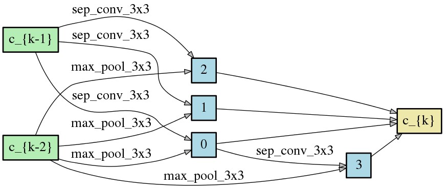
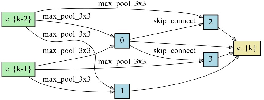
Figure 2: Cell-based architectures. Example of a normal cell (top) and a reduction cell (bottom) in the DARTS and MANAS search space. Each cell has $2$ input (green), $4$ internal (blue) and $1$ output node (yellow). Multiple cells are connected in a feedforward fashion to create a DCNN.

DARTS training configuration: we follow the same experiment setting as in (Liu, Simonyan, and Yang 2019). We replace the BN layers in DARTS with IN, LN, GN, PN and BGN in both search and evaluation stage. We search for 8 cells in $50$ epochs with batch size $64$ and initial number of channels as 16. We use SGD to optimize the model weights with initial learning rate $0.025$, momentum $0.9$ and weight decay $3\times 10^{-4}$. Adam (Kingma and Ba 2014) is used to optimize architecture parameters with initial learning rate $3\times 10^{-4}$, momentum $(0.5,0.999)$ and weight decay $10^{-3}$. We use network of 20 cells and 36 initial channels for evaluation to ensure a comparable model size as other baseline models. We use the whole training set to train the model for 600 epochs with batch size 96 to ensure convergence. For GN, we use $\rm G=32$ in (Wu and He 2018) while for BGN, we use $\rm G=256$ following Tab. 2. Other hyper-parameters are set the same as the ones in the search stage.

The best 20-cell architecture searched on CIFAR-10 by DARTS is trained from scratch with corresponding normalization methods used during the search phase. The validation accuracy of each method is reported in Tab. 3. We can see that IN and LN fails to converge while BGN out-performs GN and PN significantly and outperforms BN slightly. The accuracy of BN is re-implication of (Liu, Simonyan, and Yang 2019).

Table 3: The validation accuracy on CIFAR-10 with using BN, IN, LN, GN, PN and BGN in DARTS for the search and evaluation phase.

Normalization layer	BN	IN	LN	GN	PN	BGN
accuracy	$97.33$	-	-	$94.78$	94.41	97.40

MANAS training configuration: a single GPU is used to train the searched neural architectures (by BN) with replacing the normalization layers into BN, IN, LN, GN, PN and BGN. For GN, we use the best configuration $\rm G=32$ in (Wu and He 2018) while for BGN, we use $\rm G=64$. The network training protocol is the same as in (Carlucci et al. 2019), with the following hyperparameters: batch size $64$, epochs $600$, cutout length $16$, drop path probability $0.2$, gradient clip $5.0$, initial channels $36$, Cross-Entropy loss, SGD optimizer, learning rate decayed from $0.025$ to $0.0$, momentum $0.9$, weight decay $0.0003$.

The best 20-cell architecture searched on CIFAR-10 by MANAS is retrained from scratch with different normalization methods in place of the original BN used during the search phase. The validation accuracy of each method is reported in Tab. 4. We can see that IN, LN and PN fails to converge while BGN out-performs GN significantly and under-performs BN only slightly. It is worth noting that BN is used as the normalization layer in the neural architecture search phase, hence BN is at an advantage in this comparison.

Table 4: The validation accuracy on CIFAR-10 with replacing the normalization layer in the nerual architecture searched by MANAS to BN, IN, LN, GN, PN and BGN.

Normalization layer	BN	IN	LN	GN	PN	BGN
accuracy	97.18	-	-	$95.52$	-	$97.15$

DARTS experiment shows that BGN is generalizable to NAS for both search and evaluation. MANAS experiment shows that BGN is generalizable to less-regular neural architectures searched from NAS method.

Adversarial Training on CIFAR-10

DCNNs have been known to be vulnerable to malicious perturbed examples, known as adversarial attacks. Adversarial training was proposed to counter this problem. In this experiment, we apply BGN to adversarial training and compare its performance to BN, IN, LN, GN, and PN.

Implementation details: the WideResNet (Zagoruyko and Komodakis 2016) with the depth set as 10 and the wide factor set as 2 is used for image classification tasks on the CIFAR-10. The neural network is trained and evaluated against a four-step Projected Gradient Descent (PGD) attack. For the PGD attack, we set the step size as $2/255$, and the maximum perturbation norm as 0.0157. 200 epochs are trained until convergence. Due to the specialty of adversarial training, $\rm G=128$ is used in GN and BGN. It will divide images into patches, which can help to improve the robustness by breaking the correlation of adversarial attacks in different image blocks and constraining the adversarial attacks on the features within a limited range. This effect holds some similarity to the spectral normalization in (Farnia, Zhang, and Tse 2019). In the experiment, we use the Adam optimizer with a learning rate of 0.01.

The robust and clean accuracy of training WideResNet with BN, IN, LN, GN, PN and BGN as the normalization layer are shown in Tab. 5. The robust accuracy is more important than the clean accuracy in judging an adversarial network. PN experiences convergence difficulty and fails to converge. BGN out-performs BN and IN with a certain margin and out-performs LN and GN significantly.

Table 5: The robust and clean validation accuracy of adversarial training with BN, IN, LN, GN, PN and BGN as the normalization layer in WideResNet. The clean/robust accuracy is evaluated on the clean/PGD attacked data.

Accuracy	BN	IN	LN	GN	PN	BGN
robust accuracy	48.79	48.45	44.15	44.38	$-$	49.64
clean accuracy	72.09	72.35	64.1	68.96	$-$	72.94

Few Shot Learning

We evaluate BGN on FSL task. FSL aims to train models capable of recognizing new, previously unseen categories using only limited training samples. Basically, a training dataset with sufficient annotated samples comprise base categories. The test dataset contains $C$ novel classes, each of which is associated with only a few $K$ labelled samples (e.g. $\leq 5$ samples) compose the support set, while the remaining unlabelled samples consist the query set are used for evaluation (See Fig. 3). This is also referred to as a $C$-way $K$-shot FSL classification problem.

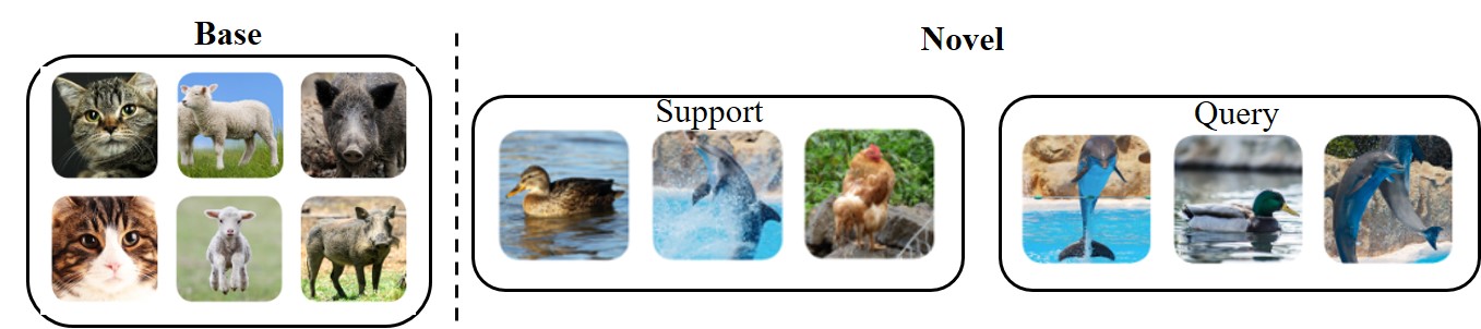
Figure 3: The illustration of FSL classification problem. The base category contains sufficient labelled samples, while the model aims at generalizing well on the novel category in the query set with limited labelled samples available in support set.

Implementation details: we experiment with imprinted weights (Qi, Brown, and Lowe 2018) model, which is one of the state-of-art metric-based FSL approaches and is widely used as the baseline in the current FSL community (Lifchitz et al. 2019; Su, Maji, and Hariharan 2019; Gidaris and Komodakis 2018). At training time, a cosine classifier is learned on top of feature extraction layers and each column of classifier parameter weights can be regarded as a prototype for the respective class. At test time, a new class prototype (new column of classifier weight parameters) is defined by averaging the feature representation of support images, and the unlabelled images are classified via a nearest neighbor strategy. We test different settings, including 5-way 1-shot and 5-way 5-shot for the ResNet-12 backbone (Oreshkin, López, and Lacoste 2018) on miniImageNet (Vinyals et al. 2016). We use the training protocol described in (Gidaris and Komodakis 2018): our model is optimized using SGD with Nesterov momentum set to $0.9$, weight decay to 0.0005, mini-batch size to 256, and 60 epochs. All input images were resized to $84\times 84$. The learning rate was initialized to 0.1, and changed to 0.006, 0.0012, and 0.00024 at the 20th, 40th and 50th, respectively.

The mean accuracy of replacing the normalization layers in Imprinted Weights to BN, IN, LN, GN, PN and BGN, of training on miniImageNet, and of the 5-way 1-shot and 5-shot tasks are shown Tab. 6. We can see that BGN out-performs BN slightly while out-performs IN, LN, GN and PN significantly, indicating the generalizability of BGN when the very limited labeled data is available.

Table 6: The mean accuracy of the 5-way 1-shot and 5-shot tasks on miniImageNet of Imprinted Weights with using ResNet-12 as a backbone. The normalization layer is replaced to BN, IN, LN, GN, PN and BGN. The mean accuracy of 600 randomly generated test episodes with 95% confidence intervals is reported.

Model	BN	IN	LN	GN	PN	BGN
1-shot	59.30	52.17	57.82	56.55	56.59	59.50
5-shot	76.22	70.49	74.87	73.20	73.89	76.32

Unsupervised Domain Adaptation on Office-31

UDA aims to learn models on a target domain while annotations are only accessible in a related source domain. Normalization layers have effect of aligning feature distributions and reducing the domain gap (Li et al. 2016; Cariucci et al. 2017). We evaluate BGN and other normalization layers on a widely adopted UDA benchmark Office-31 (Saenko et al. 2010), which consists of 4110 images belonging to 31 classes, with three different domains: Amazon, Webcam and Digital SLR camera (DSLR). CAN (Kang et al. 2019) is adopted as our model with replacing original BN with different normalization layers.

Implementation details: we follow the official released code’s implementation of CAN and use ImageNet-pretrained ResNet-50 as the model’s backbone. For tasks da (from domain DSLR to Amazon), wa and wd, the hyper-parameter $\rm G$ is set to 512. For ad and aw, we reduce $\rm G$ to 1 and 8 relatively as the source domain Amazon’s backgrounds are totally white and may result in noisy statistics when the group size is small. For dw, $\rm G$ is set to 32. We use Adam optimizer to optimize our model (Kingma and Ba 2014). The learning rate is set to 0.001 and exponential learning rate decay is applied with decay rate 0.1 and decay step 25. The mini-batch size is set to 30. The training stops when the distance between source and target features’ center is smaller than 0.001.

The results of BN, IN, LN, GN, PN and BGN are summarized in Table 7. We can see that BGN outperforms other normalization layers in most adaptation tasks, especially in wa with an $1.5\%$ accuracy improvement.

Table 7: The adaptation accuracy on Office-31 of CAN model with BN, IN, LN, GN, PN and BGN as the normalization layer. The result of each entry is averaged by three runs.

model	ad	da	wa	aw	dw	wd	mean
BN	94.8	77.2	76.1	94.2	98.4	99.7	90.1
BGN	95.2	78.5	78.5	94.2	99.1	99.9	90.9
GN	90.0	77.2	77.2	91.1	96.9	99.1	88.6
IN	88.0	76.1	75.4	90.0	97.2	98.5	87.5
LN	92.8	76.8	76.0	91.1	97.8	98.7	88.9
PN	90.9	76.5	77.1	90.6	97.8	99.5	88.7

Conclusion

BGN is proposed with good performance, stability and generalizability and without using additional trainable parameters, information across multiple layers or iterations, or extra computation. BGN facilitates the noisy/confused statistic calculation in BN with adaptively introducing feature instances from the grouped (channel, height and width) dimensions and uses a hyper-parameter $\rm G$ to control the size of divided feature groups. It is intuitive to implement, is orthogonal to and can be used in addition to many methods reviewed in Related Work to further improve performance.

References

- Arora, Lyu, and Li (2019) Arora, S.; Lyu, K.; and Li, Z. 2019. Theoretical analysis of auto rate-tuning by batch normalization. In ICLR.
- Arpit et al. (2016) Arpit, D.; Zhou, Y.; Kota, B.; and Govindaraju, V. 2016. Normalization Propagation: A Parametric Technique for Removing Internal Covariate Shift in Deep Networks. In ICML, 1168–1176.
- Ba, Kiros, and Hinton (2016) Ba, J. L.; Kiros, J. R.; and Hinton, G. E. 2016. Layer normalization. NeurIPS Deep Learning Symposium .
- Bjorck et al. (2018) Bjorck, N.; Gomes, C. P.; Selman, B.; and Weinberger, K. Q. 2018. Understanding batch normalization. In NeurIPS, 7694–7705.
- Cai, Li, and Shen (2019) Cai, Y.; Li, Q.; and Shen, Z. 2019. A Quantitative Analysis of the Effect of Batch Normalization on Gradient Descent. In ICML, 882–890.
- Cariucci et al. (2017) Cariucci, F. M.; Porzi, L.; Caputo, B.; Ricci, E.; and Bulo, S. R. 2017. Autodial: Automatic domain alignment layers. In ICCV, 5077–5085. IEEE.
- Carlucci et al. (2019) Carlucci, F.; Esperança, P. M.; Singh, M.; Yang, A.; Gabillon, V.; Xu, H.; Chen, Z.; and Wang, J. 2019. MANAS: Multi-agent neural architecture search. arxiv:1909.01051 .
- Chang et al. (2019) Chang, W.-G.; You, T.; Seo, S.; Kwak, S.; and Han, B. 2019. Domain-Specific Batch Normalization for Unsupervised Domain Adaptation. In CVPR, 7354–7362.
- Chen et al. (2018) Chen, Z.; Badrinarayanan, V.; Lee, C.-Y.; and Rabinovich, A. 2018. GradNorm: Gradient Normalization for Adaptive Loss Balancing in Deep Multitask Networks. In ICML, 794–803.
- Cho and Lee (2017) Cho, M.; and Lee, J. 2017. Riemannian approach to batch normalization. In NeurIPS, 5225–5235.
- Cooijmans et al. (2016) Cooijmans, T.; Ballas, N.; Laurent, C.; Gülçehre, Ç.; and Courville, A. 2016. Recurrent batch normalization. ICLR .
- Data et al. (2018) Data, G. W. P.; Ngu, K.; Murray, D. W.; and Prisacariu, V. A. 2018. Interpolating Convolutional Neural Networks Using Batch Normalization. In ECCV, 591–606. Springer.
- De and Smith (2020) De, S.; and Smith, S. L. 2020. Batch normalization biases deep residual networks towards shallow paths. arXiv preprint arXiv:2002.10444 .
- Deecke, Murray, and Bilen (2019) Deecke, L.; Murray, I.; and Bilen, H. 2019. Mode Normalization. In ICLR. URL https://openreview.net/forum?id=HyN-M2Rctm.
- Deng et al. (2009) Deng, J.; Dong, W.; Socher, R.; Li, L.-J.; Li, K.; and Fei-Fei, L. 2009. Imagenet: A large-scale hierarchical image database. In CVPR, 248–255. Ieee.
- (16) Everingham, M.; Van Gool, L.; Williams, C. K. I.; Winn, J.; and Zisserman, A. ???? The PASCAL Visual Object Classes Challenge 2012 (VOC2012) Results. http://www.pascal-network.org/challenges/VOC/voc2012/workshop/index.html.
- Fan (2017) Fan, L. 2017. Revisit fuzzy neural network: Demystifying batch normalization and ReLU with generalized hamming network. In NeurIPS, 1923–1932.
- Farnia, Zhang, and Tse (2019) Farnia, F.; Zhang, J.; and Tse, D. 2019. Generalizable Adversarial Training via Spectral Normalization. In ICLR. URL https://openreview.net/forum?id=Hyx4knR9Ym.
- Gidaris and Komodakis (2018) Gidaris, S.; and Komodakis, N. 2018. Dynamic few-shot visual learning without forgetting. In CVPR.
- Goyal et al. (2017) Goyal, P.; Dollár, P.; Girshick, R.; Noordhuis, P.; Wesolowski, L.; Kyrola, A.; Tulloch, A.; Jia, Y.; and He, K. 2017. Accurate, large minibatch sgd: Training imagenet in 1 hour. arXiv preprint arXiv:1706.02677 .
- He et al. (2016) He, K.; Zhang, X.; Ren, S.; and Sun, J. 2016. Deep residual learning for image recognition. In CVPR, 770–778.
- Hoffer et al. (2018) Hoffer, E.; Banner, R.; Golan, I.; and Soudry, D. 2018. Norm matters: efficient and accurate normalization schemes in deep networks. In NeurIPS, 2160–2170.
- Hou et al. (2019) Hou, L.; Zhu, J.; Kwok, J.; Gao, F.; Qin, T.; and Liu, T.-y. 2019. Normalization Helps Training of Quantized LSTM. In NeurIPS, 7344–7354.
- Huang et al. (2017) Huang, L.; Liu, X.; Liu, Y.; Lang, B.; and Tao, D. 2017. Centered weight normalization in accelerating training of deep neural networks. In ICCV, 2803–2811.
- Huang et al. (2018) Huang, L.; Yang, D.; Lang, B.; and Deng, J. 2018. Decorrelated batch normalization. In CVPR, 791–800.
- Huang et al. (2019) Huang, L.; Zhou, Y.; Zhu, F.; Liu, L.; and Shao, L. 2019. Iterative normalization: Beyond standardization towards efficient whitening. In CVPR, 4874–4883.
- Huang and Belongie (2017) Huang, X.; and Belongie, S. 2017. Arbitrary style transfer in real-time with adaptive instance normalization. In ICCV, 1501–1510.
- Ioffe (2017) Ioffe, S. 2017. Batch renormalization: Towards reducing minibatch dependence in batch-normalized models. In NeurIPS, 1945–1953.
- Ioffe and Szegedy (2015) Ioffe, S.; and Szegedy, C. 2015. Batch Normalization: Accelerating Deep Network Training by Reducing Internal Covariate Shift. In ICML, 448–456.
- Jia, Chen, and Chen (2019) Jia, S.; Chen, D.-J.; and Chen, H.-T. 2019. Instance-Level Meta Normalization. In CVPR, 4865–4873.
- Kang et al. (2019) Kang, G.; Jiang, L.; Yang, Y.; and Hauptmann, A. G. 2019. Contrastive adaptation network for unsupervised domain adaptation. In CVPR, 4893–4902.
- Kingma and Ba (2014) Kingma, D. P.; and Ba, J. 2014. Adam: A method for stochastic optimization. arXiv preprint arXiv:1412.6980 .
- Krizhevsky, Sutskever, and Hinton (2012) Krizhevsky, A.; Sutskever, I.; and Hinton, G. E. 2012. Imagenet classification with deep convolutional neural networks. In NeurIPS, 1097–1105.
- Li et al. (2019a) Li, B.; Wu, F.; Weinberger, K. Q.; and Belongie, S. 2019a. Positional Normalization. In NeurIPS, 1620–1632.
- Li et al. (2018a) Li, P.; Xie, J.; Wang, Q.; and Gao, Z. 2018a. Towards faster training of global covariance pooling networks by iterative matrix square root normalization. In CVPR, 947–955.
- Li et al. (2019b) Li, X.; Chen, S.; Hu, X.; and Yang, J. 2019b. Understanding the disharmony between dropout and batch normalization by variance shift. In CVPR, 2682–2690.
- Li and Vasconcelos (2019) Li, Y.; and Vasconcelos, N. 2019. Efficient Multi-Domain Learning by Covariance Normalization. In CVPR, 5424–5433.
- Li et al. (2018b) Li, Y.; Wang, N.; Shi, J.; Hou, X.; and Liu, J. 2018b. Adaptive batch normalization for practical domain adaptation. PR 80: 109–117.
- Li et al. (2016) Li, Y.; Wang, N.; Shi, J.; Liu, J.; and Hou, X. 2016. Revisiting batch normalization for practical domain adaptation. arXiv preprint arXiv:1603.04779 .
- Lifchitz et al. (2019) Lifchitz, Y.; Avrithis, Y.; Picard, S.; and Bursuc, A. 2019. Dense Classification and Implanting for Few-Shot Learning. CVPR .
- Lin et al. (2014) Lin, T.-Y.; Maire, M.; Belongie, S.; Hays, J.; Perona, P.; Ramanan, D.; Dollár, P.; and Zitnick, C. L. 2014. Microsoft coco: Common objects in context. In ECCV, 740–755. Springer.
- Liu, Simonyan, and Yang (2019) Liu, H.; Simonyan, K.; and Yang, Y. 2019. DARTS: Differentiable Architecture Search. In International Conference on Learning Representations. URL https://arxiv.org/abs/1806.09055.
- Luo et al. (2019a) Luo, P.; Ren, J.; Peng, Z.; Zhang, R.; and Li, J. 2019a. Differentiable Learning-to-Normalize via Switchable Normalization. In ICLR. URL https://openreview.net/forum?id=ryggIs0cYQ.
- Luo et al. (2019b) Luo, P.; Wang, X.; Shao, W.; and Peng, Z. 2019b. Towards Understanding Regularization in Batch Normalization. In ICLR. URL https://openreview.net/forum?id=HJlLKjR9FQ.
- Luo et al. (2019c) Luo, P.; Zhang, R.; Ren, J.; Peng, Z.; and Li, J. 2019c. Switchable normalization for learning-to-normalize deep representation. TPAMI .
- Miyato et al. (2018) Miyato, T.; Kataoka, T.; Koyama, M.; and Yoshida, Y. 2018. Spectral normalization for generative adversarial networks. arXiv preprint arXiv:1802.05957 .
- Nam and Kim (2018) Nam, H.; and Kim, H.-E. 2018. Batch-instance normalization for adaptively style-invariant neural networks. In NeurIPS, 2558–2567.
- Oreshkin, López, and Lacoste (2018) Oreshkin, B.; López, P. R.; and Lacoste, A. 2018. Tadam: Task dependent adaptive metric for improved few-shot learning. In NeurIPS.
- Park et al. (2019) Park, T.; Liu, M.-Y.; Wang, T.-C.; and Zhu, J.-Y. 2019. Semantic image synthesis with spatially-adaptive normalization. In CVPR, 2337–2346.
- Qi, Brown, and Lowe (2018) Qi, H.; Brown, M.; and Lowe, D. G. 2018. Low-shot learning with imprinted weights. In CVPR, 5822–5830.
- Ren et al. (2016) Ren, M.; Liao, R.; Urtasun, R.; Sinz, F. H.; and Zemel, R. S. 2016. Normalizing the normalizers: Comparing and extending network normalization schemes. ICLR .
- Saenko et al. (2010) Saenko, K.; Kulis, B.; Fritz, M.; and Darrell, T. 2010. Adapting visual category models to new domains. In ECCV, 213–226. Springer.
- Salimans and Kingma (2016) Salimans, T.; and Kingma, D. P. 2016. Weight normalization: A simple reparameterization to accelerate training of deep neural networks. In NeurIPS, 901–909.
- Santurkar et al. (2018) Santurkar, S.; Tsipras, D.; Ilyas, A.; and Madry, A. 2018. How does batch normalization help optimization? In NeurIPS, 2483–2493.
- Shao et al. (2019) Shao, W.; Meng, T.; Li, J.; Zhang, R.; Li, Y.; Wang, X.; and Luo, P. 2019. Ssn: Learning sparse switchable normalization via sparsestmax. In CVPR, 443–451.
- Singh and Shrivastava (2019) Singh, S.; and Shrivastava, A. 2019. EvalNorm: Estimating Batch Normalization Statistics for Evaluation. In ICCV, 3633–3641.
- Su, Maji, and Hariharan (2019) Su, J.-C.; Maji, S.; and Hariharan, B. 2019. Boosting Supervision with Self-Supervision for Few-shot Learning. arXiv .
- Summers and Dinneen (2019) Summers, C.; and Dinneen, M. J. 2019. Four Things Everyone Should Know to Improve Batch Normalization. arXiv preprint arXiv:1906.03548 .
- Ulyanov, Vedaldi, and Lempitsky (2016) Ulyanov, D.; Vedaldi, A.; and Lempitsky, V. 2016. Instance normalization: The missing ingredient for fast stylization. arXiv preprint arXiv:1607.08022 .
- Vinyals et al. (2016) Vinyals, O.; Blundell, C.; Lillicrap, T.; Wierstra, D.; et al. 2016. Matching networks for one shot learning. In NeurIPS.
- Wang et al. (2018) Wang, G.; Luo, P.; Wang, X.; Lin, L.; et al. 2018. Kalman normalization: Normalizing internal representations across network layers. In NeurIPS, 21–31.
- Wang et al. (2019) Wang, X.; Jin, Y.; Long, M.; Wang, J.; and Jordan, M. I. 2019. Transferable Normalization: Towards Improving Transferability of Deep Neural Networks. In NeurIPS, 1951–1961.
- Wu and He (2018) Wu, Y.; and He, K. 2018. Group normalization. In ECCV, 3–19.
- Xu et al. (2019a) Xu, J.; Sun, X.; Zhang, Z.; Zhao, G.; and Lin, J. 2019a. Understanding and Improving Layer Normalization. In NeurIPS, 4383–4393.
- Xu et al. (2019b) Xu, Y.; Duan, J.; Kuang, Z.; Yue, X.; Sun, H.; Guan, Y.; and Zhang, W. 2019b. Geometry Normalization Networks for Accurate Scene Text Detection. In ICCV, 9137–9146.
- Yan et al. (2019) Yan, J.; Wan, R.; Zhang, X.; Zhang, W.; Wei, Y.; and Sun, J. 2019. Towards Stabilizing Batch Statistics in Backward Propagation of Batch Normalization. In ICLR.
- Yang et al. (2019) Yang, G.; Pennington, J.; Rao, V.; Sohl-Dickstein, J.; and Schoenholz, S. S. 2019. A Mean Field Theory of Batch Normalization. In ICLR. URL https://openreview.net/forum?id=SyMDXnCcF7.
- Zagoruyko and Komodakis (2016) Zagoruyko, S.; and Komodakis, N. 2016. Wide Residual Networks. In Richard C. Wilson, E. R. H.; and Smith, W. A. P., eds., BMVC, 87.1–87.12. BMVA Press. ISBN 1-901725-59-6. doi:10.5244/C.30.87. URL https://dx.doi.org/10.5244/C.30.87.
- Zhang and Sennrich (2019) Zhang, B.; and Sennrich, R. 2019. Root Mean Square Layer Normalization. In NeurIPS, 12360–12371.
- Zhang, Dauphin, and Ma (2019) Zhang, H.; Dauphin, Y. N.; and Ma, T. 2019. Residual Learning Without Normalization via Better Initialization. In ICLR. URL https://openreview.net/forum?id=H1gsz30cKX.
- Zhou (2019) Zhou, X. 2019. 3D shape instantiation for intra-operative navigation from a single 2D projection .
- Zhou et al. (2019) Zhou, X.-Y.; Li, P.; Wang, Z.-Y.; and Yang, G.-Z. 2019. U-net training with instance-layer normalization. In International Workshop on Multiscale Multimodal Medical Imaging, 101–108. Springer.
- Zhou and Yang (2019) Zhou, X.-Y.; and Yang, G.-Z. 2019. Normalization in training U-Net for 2-D biomedical semantic segmentation. IEEE Robotics and Automation Letters 4(2): 1792–1799.