Relativistic time-dependent quantum dynamics across supercritical barriers for Klein-Gordon and Dirac particles

Abstract

We investigate wavepacket dynamics across supercritical barriers for the Klein-Gordon and Dirac equations. Our treatment is based on a multiple scattering expansion (MSE). For spin-0 particles, the MSE diverges, rendering invalid the use of the usual connection formulas for the scattering basis functions. In a time-dependent formulation, the divergent character of the MSE naturally accounts for charge creation at the barrier boundaries. In the Dirac case, the MSE converges and no charge is created. We show that this time-dependent charge behavior dynamics can adequately explain the Klein paradox in a first quantized setting. We further compare our semi-analytical wavepacket approach to exact finite-difference solutions of the relativistic wave equations.

I Introduction

One of the salient features of relativistic quantum mechanics is the intrinsic mixture of particles with their corresponding antiparticles. This aspect already appears in "first quantized" single particle Relativistic Quantum Mechanics (RQM) greiner . This phenomenon becomes prominent when a particle is placed in a very strong external classical field, a field strong enough to close the gap between particles and antiparticles – a supercritical field.

Most textbooks, as well as the overwhelming majority of past works employ time-independent stationary phase or plane wave arguments when dealing with supercritical fields within RQM. As is well known, in quantum scattering theory time-independent quantities such as cross-sections or energy levels can be readily computed, but it is often ambiguous to attempt to infer the dynamics from considerations involving a single plane wave. This is even more the case when relativistic phenomena are investigated: one has to deal with additional difficulties, such as the breakdown of the usual connection formulas linking the scattering solutions in different regions, or the Klein paradox – a phenomenon usually expressed as a current reflected from a supercritical step or barrier higher than the incident one. Standard textbooks (e.g. bjorken ; greiner ; strange ; wachter ) give different, often conflicting accounts of the Klein paradox. This situation is reflected even in recent works DiracSpin ; kim2019 ; morales19 ; xue ; no-klein-tunnel-dirac ; noKP-Dirac ; bosanac ; emilio ; leo2006 ; noKP-KG ; nitta , that reach different conclusions generally based on time independent considerations.

In part for this reason, it is often stated, in different situations dealing with the Klein paradox, that a RQM approach is inadequate and that a quantum field theory (QFT) treatment is necessary (see e.g. strange for the step case, or xue for the barrier case). Nevertheless even in a first quantized framework the RQM wave equations have charge creation built-in. We argue in this paper that this aspect is best understood by considering the time-dependent wavefunction dynamics. We will assess whether this leads to a consistent first quantized explanation of the Klein paradox. Interestingly, other very recent works have focused on different time-dependent aspects of the relativistic wave equations transient ; KG-moving .

In this paper we will develop a time-dependent wavepacket treatment suited to investigate the dynamics of spin-0 bosons and spin-1/2 fermions in model supercriticial barriers. In order to develop our semi-analytic wavepacket approach, we will rely on a Multiple Scattering Expansion (MSE). We will see that the nature of the MSE is different for solutions of the Klein-Gordon and Dirac equations. In the Klein-Gordon case, the MSE diverges, physically corresponding to charge creation as the wavepacket hits a barrier’s edge. This implies that the usual connection formulas between wavefunctions in different regions – which are obeyed when a single step potential is considered – are not applicable when dealing with supercritical barriers. Employing connection formulas leads to inconsistencies, like superluminal traversal times, that were recently noted xue though (incorrectly, as we will see) attributed to the limitations of the first quantized formalism. In the Dirac case, the MSE converges, as no charge is created when the wavepacket hits the barrier. This leads to an interpretation of Klein tunneling that is qualitatively different from the bosonic case. This also ensures that the connection formulas, that have been employed in a countless number of works, remain valid.

The multiple scattering expansion will be given in Sec. II, after introducing the model barriers we will be working with. These ingredients will be employed in Sec. III to build wavepackets. We will then give a couple of examples displaying the dynamics of a bosonic or fermionic particle impinging on a supercritical barrier. Our wavepacket results will be compared to numerical solutions obtained from a code we have developed to solve numerically the relativistic wave equations. Our results will be discussed in Sec. IV. We will more specifically focus on the extent to which the Klein paradox can be accounted for within a first quantized framework. We close the paper by a Conclusion.

II Charge creation and Multiple Scattering Expansions

II.1 Potential barriers

We are interested in this work by the dynamics of a relativistic “particle” impinging on a one dimensional static barrier of width $L$. The barrier should be discriminated from the step, which is by far the case that has most often been considered in studies of the Klein paradox. The relevant wave equations for spin-0 and spin-1/2 particles are recalled in Appdx A.

The simplest case is the rectangular barrier defined by $V(x)=V\theta(x)\theta(L-x)$ where $\theta$ denotes the unit-step function and $V$ denotes the barrier height. We will also consider smooth barriers, for which we will employ the potential $V_{s}(x,\epsilon)=\frac{V}{2}\left[\tanh(\epsilon x)-\tanh\left(\epsilon(x-L)\right)\right]$ since for this potential analytical solutions are known kennedy ; $\epsilon$ is the smoothness parameter.

II.1.1 Subcritical barriers

Let us consider a rectangular barrier. Plane wave solutions of the canonical KG equation (see Appdx A) are of the form

$$\psi_{j}^{\pm}(t,x)=\left(A_{j}^{\pm}e^{ip_{j}x/\hbar}+B_{j}^{\pm}e^{-ip_{j}x/\hbar}\right)e^{\mp iE(p_{1})t/\hbar}$$ (1)

where $j=1,2,3$ denotes the regions depicted in Fig. 1 and the $\pm$ signs corresponds to states with positive and negative energies $\pm E(p_{1})$ with $E(p_{1})=\sqrt{m^{2}c^{4}+p_{1}^{2}c^{2}}$. $p_{j}$ is the momentum; for positive energies, $p_{j}>0$ gives a wave moving from left to right (but from right to left for negative energies).

As is well known manogue ; greiner , for “subcritical” potentials ($p_{2}$ is imaginary) plane-waves scattering is similar to the usual non-relativistic situation (small transmission amplitude and exponentially decreasing waves). Assume boundary conditions for which an incident positive energy wave travels from left to right; this imposes $B_{3}=0$ and for definiteness we set the incoming amplitude to $A_{1}=1$. The other amplitudes $A_{j}$ and $B_{j}$ are deduced by matching the wavefunctions and their space derivatives at the boundaries $x=0$ and $x=L$ (for reasons that will become clear below, we will not need to deal with boundary conditions for negative energy plane waves; we henceforth write $A$ for $A^{+},$ etc.). This way of obtaining the amplitudes does not necessarily hold when $V$ becomes supercritical.

II.1.2 Supercritical barriers

A supercritical potential is a potential high enough to give rise to Klein tunneling review99 , whereby the incoming wavepacket penetrates undamped ($p_{2}$ is real) inside the barrier. In the bosonic case, this gives rise manogue to superradiance (a reflected current higher than the incoming one). In the fermionic case there is no superradiance (although some authors suggest differently, see e.g. bjorken ; leo2006 ), and supercritical steps have been deemed to have an acceptable interpretation only within a QFT approach hansen ; grobe-review ; gavrilov , a point that appears to be supported by the wide variety of conflicting interpretations of Klein tunneling that have been proposed within the first quantized framework DiracSpin ; kim2019 ; morales19 ; xue ; no-klein-tunnel-dirac ; noKP-Dirac ; bosanac ; emilio ; leo2006 ; noKP-KG ; nitta .

II.2 Multiple Scattering Expansions

It is well-known that when transmission of waves across several media takes place, one has to take into account a multiple scattering process. Referring again to Fig. 1, consider an asymptotically free (at $x=-\infty$) wave coming toward the barrier (we set again $A_{1}=1$ and $B_{3}=0$). Reflection of the incoming wave on the barrier takes place with amplitude $r_{l}^{i}$, which is the reflection amplitude of a step. The transmitted amplitude at that point, $t_{l}^{i}$ is that of a step, but the wave traveling inside the barrier reaches the right edge and gets transmitted and reflected with amplitudes $t_{r}^{i}$ and $r_{r}^{i}$. This reflected wave travels back towards the left side of the barrier, getting reflected and transmitted with coefficients $r_{l}^{o}$ and $t_{l}^{o}$. This process is iterated an infinite number of times yielding

$$r\equiv B_{1}=r_{l}^{i}+t_{l}^{i}t_{l}^{o}r_{r}^{i}\sum_{n\geq 0}(r_{l}^{o}r_{r}^{i})^{n}\quad$$

       (2)

The amplitudes obtained by using this Multiple Scattering Expansion (MSE) should match those obtained by employing the usual connection formulas at the boundaries, but this will happen only provided the sums in Eq. (2) converge.

II.2.1 Klein-Gordon equation: Divergent Multiple Scattering Expansion

Let us consider the KG equation in the presence of a supercritical step $V\theta(x)$ at $x=0$. Scattering of a positive energy plane wave coming from the left, as given by Eq. (1) sets $\bar{A}_{1}=1,\bar{B}_{2}=0$ (we use the bar to avoid confusion between the step and barrier amplitudes). $\bar{A}_{2}$ and $\bar{B}_{1}$ are thus obtained by applying the boundary conditions at $x=0$, yielding $\bar{B}_{1}=(p_{1}-p_{2})/(p_{1}+p_{2})$ and $\bar{A}_{2}=2p_{1}/(p_{1}+p_{2})$ where following our notation given above, $p_{1}>0$ is the momentum of the incoming plane wave (in region 1) and

$$p_{2}(p_{1})=-\frac{1}{c}\sqrt{p_{1}^{2}c^{2}-2V\left(m^{2}c^{4}+p_{1}^{2}c^{2}\right)^{1/2}+V^{2}}.$$ (3)

The amplitudes $\bar{B}_{1}$ and $\bar{A}_{2}$ of the step correspond to the amplitudes $r_{l}^{i}$ and $t_{l}^{i}$ of the barrier MSE, Eq. (2). $r_{r}^{i}$ and $t_{r}^{i}$ are obtained by considering the step $V\theta\left(L-x\right)$, and $r_{l}^{o}$ and $t_{l}^{o}$ arise from the step $V\theta(x)$ with a wave coming from the right (see Appdx B). By inserting the values for these elementary scattering amplitudes into the MSE of Eq. (2), we obtain the scattering amplitudes for the rectangular barrier. These amplitudes converge if $|(p_{1}-p_{2})/(p_{1}+p_{2})|<1$ in which case it can be checked that the amplitudes $A_{j}$ and $B_{j}$ match the ones obtained by using the connection formulas at the boundaries.

This condition is fulfilled for subcritical barriers (both $p_{1}$ and $p_{2}$ are positive) but for supercritical barriers, we have $p_{1}>0$ and $p_{2}<0$ and the MSE diverges. This divergence does not make much sense in a stationary plane-wave picture, in which the scattering amplitudes become infinite, but we will see below in Sec. III that in a time-dependent approach, the divergence corresponds physically to the creation of charge each time a wavepacket hits a barrier edge.

Interestingly, if the “converged” amplitudes (usually obtained by employing the connection formulas) are employed in the supercritical case, unphysical results are obtained. It was recently noticed xue in a plane wave analysis that the barrier traversal time defined from the phase energy derivative was superluminal in the supercritical case, an unphysical result attributed to the limitations of the first quantized formalism. In a wavepacket approach, building wavepackets with the converged amplitudes results in an acausal wavepacket coming out from the right side of the supercritical barrier before the incoming wavepacket has even hit the barrier paper1 . Other works have also employed the connection formulas in a supercritical context kim2019 ; emilio .

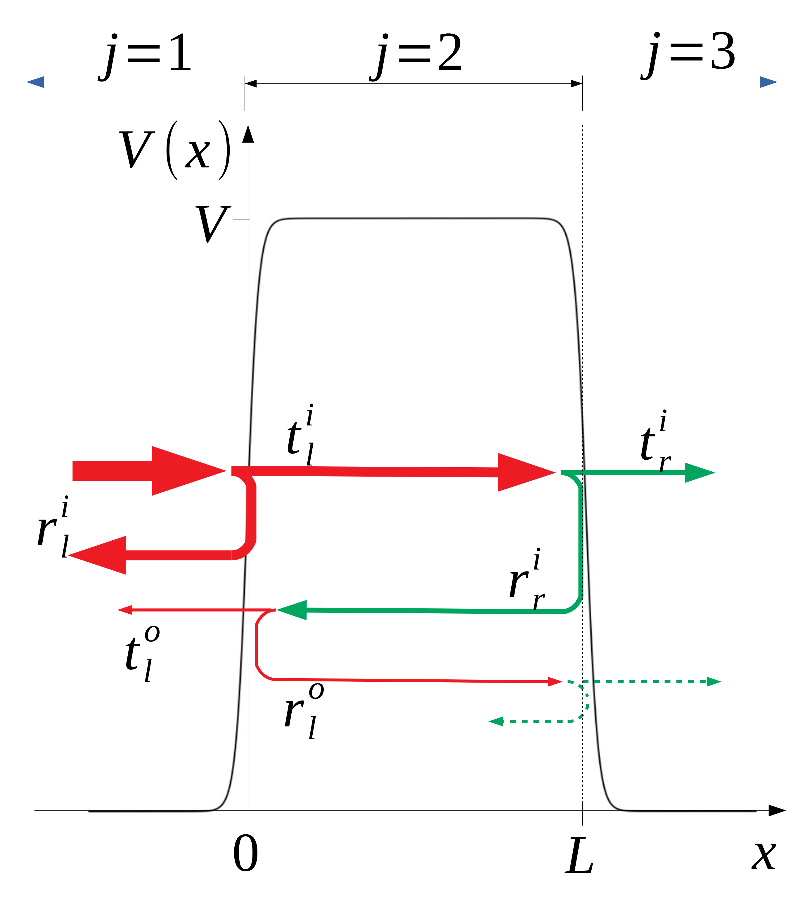
Figure 1: A generic barrier is shown along with the $3$ regions $j=1,2,3$. The scattering amplitudes of the Multiple Scattering Expansion at the left ($l$) and right ($r$) edges are indicated for an incoming wave boundary condition (see text for details).

II.2.2 Dirac equation: Convergent Multiple Scattering Expansion

The derivation of the MSE for the Dirac equation is similar to the one we have given for the KG equation. The plane wave solutions of the 2-component state $\Phi(t,x)$ take the form:

$$\Phi_{j}^{\pm}(t,x)=\left[A_{j}^{\pm}\left(\begin{array}[c]{c}1\\ \alpha_{j}^{\pm}(p_{1})\end{array}\right)e^{{}^{ip_{j}x/\hbar}}+B_{j}^{\pm}\left(\begin{array}[c]{c}1\\ -\alpha_{j}^{\pm}(p_{1})\end{array}\right)e^{{}^{-ip_{j}x/\hbar}}\right]e^{-i\sqrt{m^{2}c^{4}+p_{1}^{2}c^{2}}t/\hbar}n_{j}^{\pm}(p_{1})$$ (4)

where the coefficients $\alpha_{j}^{\pm}$ are given by Eqs. (C-5) to (C-8) of Appdx C.$j$ refers again to the 3 regions depicted in Fig. 1 and $n_{j}^{\pm}$ are normalization coefficients.

As in the KG case, let us treat the barrier as a multiple scattering expansion, with the same boundary conditions. The amplitudes $A_{j}^{\pm}$ and $B_{j}^{\pm}$ are again given by Eq. (2), with coefficients $r_{l}^{i},$ $t_{l}^{i}...$ that are different for positive and negative energy wavefunctions. As in the KG case, the MSE for a rectangular barrier is built from the reflection and transmission amplitudes $\bar{A}_{j}^{\pm}$ and $\bar{B}_{j}^{\pm}$ of the steps $V\theta(x)$ and $V\theta(L-x)$. The matching condition $\Phi_{1}^{+}(t,x=0)=\Phi_{2}^{+}(t,x=0)$, yields

$$\bar{B}_{1}^{+}=\frac{\alpha_{1}^{+}(p_{1})-\alpha_{2}^{+}(p_{1})}{\alpha_{1}^{+}(p_{1})+\alpha_{2}^{+}(p_{1})}\qquad\bar{A}_{2}^{+}=\frac{2\alpha_{1}^{+}(p_{1})}{\alpha_{1}^{+}(p_{1})+\alpha_{2}^{+}(p_{1})}\frac{n_{1}^{+}}{n_{2}^{+}}.$$ (5)

The amplitudes $\bar{B}_{1}$ and $\bar{A}_{2}$ of the step correspond to the amplitudes $r_{l}^{i+}$ and $t_{l}^{i+}$ entering the MSE for the barrier. The other step amplitudes are obtained in the same manner, see Eq. (B-5) in the Appdx. It can be seen that the series converge provided $\lvert\frac{\alpha_{1}^{+}(p_{1})-\alpha_{2}^{+}(p_{1})}{\alpha_{1}^{+}(p_{1})+\alpha_{2}^{+}(p_{1})}\rvert<1$ true since $\alpha_{2}^{+}(p_{1})$ is positive when $V$ is supercritical.

Therefore for the Dirac equation, the MSE converges. The usual connection formulas at $x=0$ and $x=L$ may be employed to obtain directly the barrier amplitudes $A_{j}^{\pm}$ and $B_{j}^{\pm}$ given by Eqs. (C-9) to (C-12). Note that most past works (e.g., emilio ; graphene ; barrierDex1 ) have indeed employed such connection formulas without however examining the justifications for their use.

III Wavepacket dynamics

III.1 Construction from plane-wave expansions

The most straightforward way to construct wavepackets starting from an initial distribution is to employ a plane-wave expansion, valid everywhere except in the slope region for a sufficiently steep barrier.

III.1.1 Klein-Gordon equation wavepackets

The Klein-Gordon plane-waves were given in Eq. (1). These solutions can be expressed in Hamiltonian form (see Appdx A), as

$$\Psi_{j}^{\pm}(t,x)=N\begin{pmatrix}mc^{2}\pm\sqrt{m^{2}c^{4}+p_{j}^{2}c^{2}}\\ mc^{2}\mp\sqrt{m^{2}c^{4}+p_{j}^{2}c^{2}}\end{pmatrix}\left(A_{j}^{\pm}e^{ip_{j}x/\hbar}+B_{j}^{\pm}e^{-ip_{j}x/\hbar}\right)e^{\mp i\sqrt{m^{2}c^{4}+p_{1}^{2}c^{2}}t/\hbar}\ ,$$ (6)

where $p_{3}=p_{1}$ and $p_{2}$ is given by Eq. (3), the amplitudes $A_{j}^{\pm}$ and $B_{j}^{\pm}$ are given by Eq. (2), and $N$ is a global normalisation constant.

Assume that at $t=0$ we have an initial wavefunction $G(t=0,x)=\left(\varphi_{G}(0,x),\chi_{G}(0,x)\right)$ in region 1, to the left of the barrier. The time evolution can be employed by applying the pseudo-unitary evolution operator on $G(t=0,x),$ or equivalently by using the Fourier transform $G(t=0,x)=\int dpe^{ipx/\hbar}\hat{G}(t=0,p).$  The time evolved wavepacket can then be written as

$$G(t,x)=\sum_{j}\theta_{j}\int dp_{1}\left(c_{KG}^{+}(p_{1})\Psi_{j}^{+}(t,x;p_{1})+c_{KG}^{-}(p_{1})\Psi_{j}^{-}(t,x;p_{1})\right),$$ (7)

where $\theta_{j}$ ensures each expression is used only in the region $j$ in which it is valid, as per Fig. 1 (explicitly, $\theta_{1}=\theta(-x),\theta_{2}=\theta(x)\theta(L-x)$ and $\theta_{3}=\theta(x-L)$).

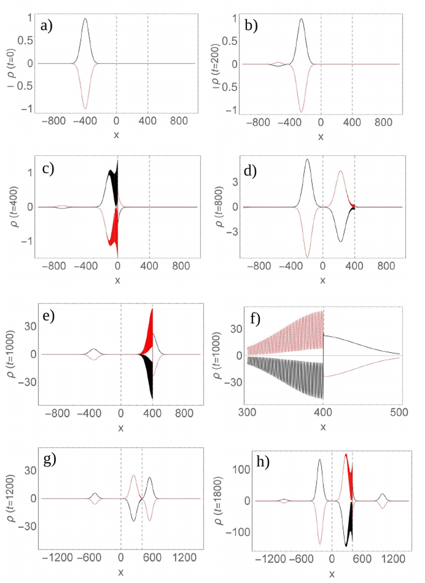
Figure 2: Wavepacket dynamics for a spin-0 boson described by the Klein Gordon equation impinging on a smooth supercritical barrier. The charge density $\rho(t)$ is given for different times as specified on each plot. Our semi-analytic wavepacket approach is shown in black solid lines, while for the sake of comparison our finite-difference solutions are shown upside-down with a dashed (online: red) line. The supercritical barrier lies within the dotted vertical gray lines. The same initial state, shown in a) is taken for the wavepacket and the numerical calculations and no adjustment or renormalization are made at longer times (the change in scale reflects charge creation). Note that f) is a zoom of e) in the region around the right edge of the barrier. The values of the parameters employed are given in the main text. Natural units ($\hbar=c=m=\varepsilon_{0}=1$) are used units .

To be specific, we will choose an initially localized state of the form

$$G(0,x)=(\exp(\frac{-(x-x_{0})^{2}}{4d^{2}}-ip_{0}x/\hbar),0)$$ (8)

Picking $x_{0}$ far to the left of the barrier and $p_{0}>0$, the choice (25) gives an initial state with positive charge. The coefficients $c_{KG}^{\pm}=\left\langle\Psi_{1}^{\pm}\right|\left.G\right\rangle_{KG}$ are readily computed [Eq. (C-4)] and it can be seen that $c_{KG}^{-}$ is non-zero (although it is small for non-relativistic velocities). This negative energy component moves to the left (recall that $p_{0}>0$ yields an antiparticle that moves in the negative direction), so only the positive energy wavepacket (particle) impinges on the barrier .

III.1.2 Dirac equation wavepackets

A similar construction can be used to build wavepackets evolving according to the Dirac equation, starting from an initial state $\left|G(t=0)\right\rangle$ of the same form as Eq. (25) now expanded over the Dirac equation plane-wave solutions. The time evolved wavepacket is

$$G(t,x)=\sum_{j}\theta_{j}\int dp_{1}\left(c_{D}^{+}(p_{1})\Phi_{j}^{+}(t,x;p_{1})+c_{D}^{-}(p_{1})\Phi_{j}^{-}(t,x;p_{1})\right),$$ (9)

where the coefficients $c_{D}^{\pm}=\left\langle\Phi_{1}^{\pm}\right|\left.G\right\rangle$ are given by Eq. (C-13).

III.2 Numerical solutions

We have computed numerical solutions to the Klein-Gordon and Dirac equations. This was done by discretizing the corresponding evolution operator in real space for small time steps. The initial wavefunction $G(t=0,x)$ is discretized on a fixed space-grid and the derivatives in the evolution operator are approximated by finite differences in the fourth or fifth-order approximation. The computational details are given in Appdx D (see also Refs. keitel ; bauke ; muller ).

III.3 Illustrative Results

We will now illustrate our wavepacket approach and compare it with fully numerical solutions obtained by solving the relativistic wave equations with a finite-difference scheme.

Fig. 2 illustrates the wavepacket dynamics for a spin-0 boson impinging on a smooth barrier $V_{s}(x,\epsilon)$ with $\epsilon=5,$ $L=400$ and $V=3.4$ (we use natural units units ). We pick the initial state Eq. (25) with $x_{0}=-400,$ $p_{0}=\sqrt{5}/2$ and $d=50$ (in order to have a rather narrow momentum distribution). We also provide numerical solutions obtained by using our finite-difference scheme introduced above (these solutions are plotted upside-down). The wavepacket moves towards the barrier (save for an antiparticle component moving to the left, visible at $t=200$), and has appreciably hit the barrier by $t=400$, while at $t=800$ one sees Klein tunneling accompanied by charge production both inside and outside the left edge of the barrier (note the vertical scale). At $t=1000$, the antiparticle wavepacket hits the right edge of the barrier, inducing additional charge production both for the transmitted (particle) wavepacket and for the reflected (antiparticle) one. This motion continues, with the amplitude inside the barrier growing at each reflection.

The MSE based wavepacket dynamics match very well the computations obtained from the finite-difference solutions. In practice, the number of terms that need to be taken into account in the MSE sum (2) is congruent with the time $t$ at which the wavepacket is computed. Indeed, the $n$th term corresponds formally to a wavepacket translated by the order of $2n\pi L$, that for values of $n$ that are high enough did not have time to reach the barrier. Hence these terms do not contribute to the wavepacket (in the calculations shown on Fig. 2, including terms up to $n=4$ is sufficient).

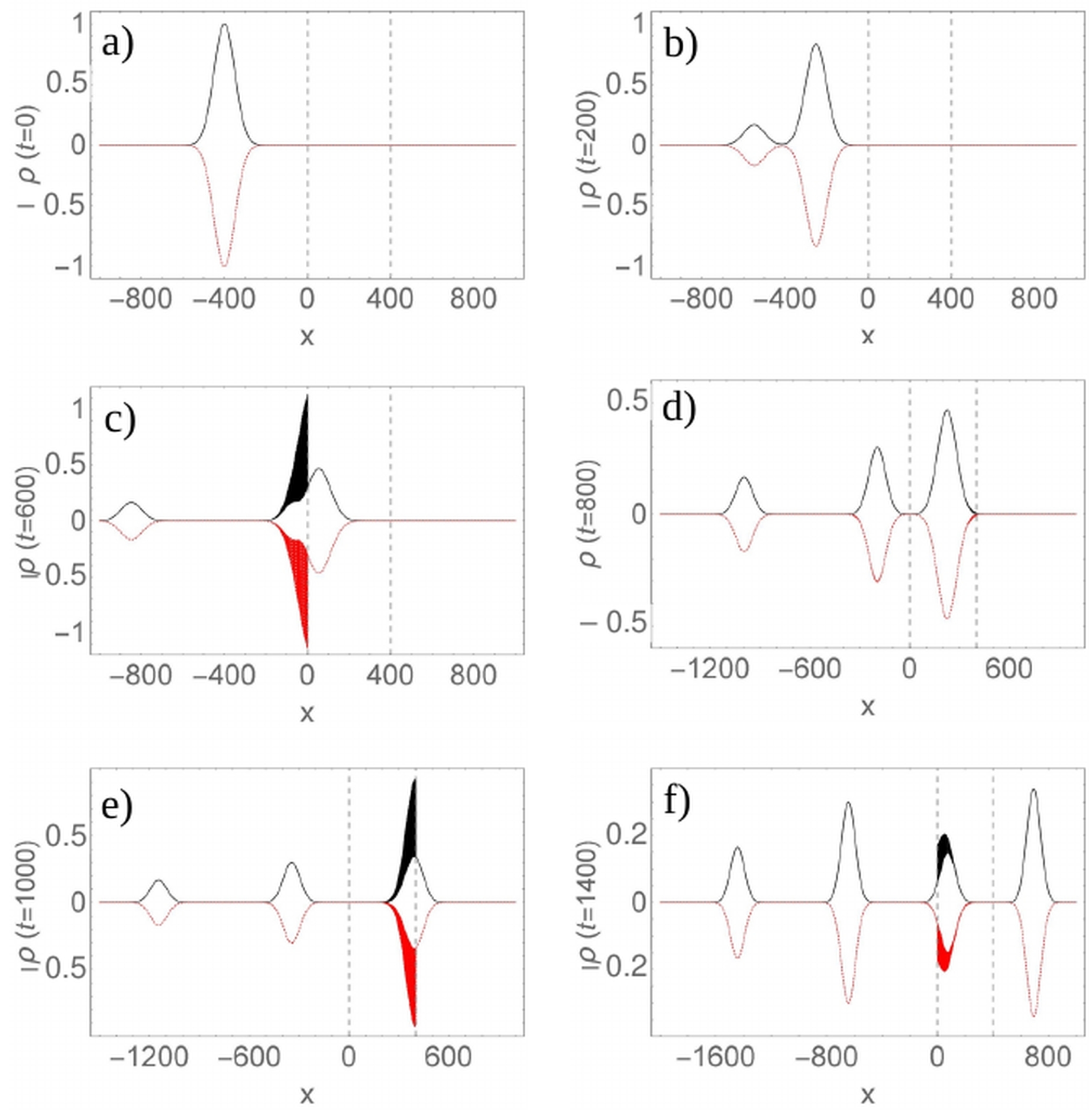
Figure 3: Wavepacket dynamics for a spin-1/2 fermion described by the Dirac equation impinging on a supercritical barrier. The density $\rho(t)$ is given for different times as specified. The semi-analytic wavepacket approach gives the results shown in black solid lines, while the finite-difference solutions are shown upside-down with a dashed (online: red) line. The supercritical barrier lies within the dotted vertical gray lines. The same initial state, shown in a) is taken for the wavepacket and the numerical calculations and no adjustment or renormalization are made at longer times. The values of the parameters employed are given in the main text. Natural units ($\hbar=m=c=\varepsilon_{0}=1$, where $m$ is the electron mass) are used.

The wavepacket dynamics for a spin 1/2 fermion is shown in Fig. 3. We picked the same barrier and initial state parameters as in the Klein-Gordon case except that the smoothness parameter was taken to be the size of the space integration step in the numerical code ($\epsilon\simeq 250$), effectively corresponding to the rectangular barrier limit. We note again the very good agreement between the wavepackets constructed with Eq. (9) and the numerical solutions.

IV Discussion

IV.1 General remarks

We have developed a wave-packet approach to describe Klein tunneling across a supercritical barrier both for Klein-Gordon and Dirac particles. The main ingredient was seen to be the multiple scattering expansion, that diverges in the KG case but converges in the Dirac case.

The main issue now is whether these results lend to a consistent interpretation of the Klein paradox within the first quantized formalism. This is known to be problematic when basing considerations on stationary plane waves, and indeed different, sometimes conflicting interpretations of superradiance and supercritical tunneling in a first quantized framework have been given DiracSpin ; kim2019 ; morales19 ; xue ; no-klein-tunnel-dirac ; noKP-Dirac ; bosanac ; emilio ; leo2006 ; noKP-KG ; nitta . Klein tunneling has even been denied to exist in the bosonic  case noKP-KG or for fermions noKP-Dirac . Of course since particle creation is induced by supercritical potentials, a proper approach requires a QFT treatment. But time-dependent QFT approaches to tackle this problem are scarce (with the exception of the work reviewed in Ref grobe-review , where supercriticial steps, rather than barriers, were investigated both for fermions and bosons; see also grobe-recent and Refs. therein for recent ramifications of this  time-dependent QFT method). Hence, although time-independent approaches to Klein tunneling within the first quantized framework might be seen as unreliable, it would be worthwhile to consider the merits of a time-dependent first quantized account, and examine its consistency with time-dependent QFT approaches.

IV.2 Klein Paradox in a first quantized framework

IV.2.1 Bosons

For the Klein-Gordon equation, the account seems rather simple: a supercritical potential creates positive and negative charges in equal amounts but in different spatial regions. In our wavepacket approach, this is explained by the divergent character of the multiple scattering expansion, although this property is encapsulated in the pseudo-unitary evolution operator that is solved numerically in the finite-difference code.

Hence, when a particle impinges on a supercritical barrier, the reflected wavepacket has a higher amplitude than the incoming one. Similarly, when the Klein tunneling wavepacket reaches the right edge of the barrier, a positively charged wavepacket leaves the barrier, and this is compensated by additional negative charge inside the barrier. This process goes on indefinitely with positive and negative charge increasing at each reflection (to the extent that the supercritical potential can be maintained despite the growing charge inside the barrier).

It is difficult to accommodate the charge creation mechanism by supercritical fields with the idea that the first quantized framework would describe a single particle in a superposition of states of different charges (rather than explaining this feature in terms of particle-antiparticle creation). However, leaving this important physical issue aside, we see that the time-dependent wavepackets by themselves do account for the bosonic Klein paradox.

IV.2.2 Fermions

For the Dirac equation, the dynamics is very different. Assume the incoming particle is an electron (with negative charge). Part of the incoming wavepacket gets reflected by the barrier, and part gets transmitted. Contrary to the bosonic case, there is no charge creation, so the reflected wavepacket has a smaller amplitude than the incoming one. Since the total probability density is conserved, requiring charge conservation implies that the wavepacket tunneling inside the barrier also has negative charge. This is difficult to accommodate within a single particle picture, even by relying on hole theory.

Indeed, according to the standard hole theory account of the Klein paradox for fermions (see Ch. 12 of greiner ), the energy levels of the Dirac sea are raised inside the barrier by the supercritical potential. The incoming electron can then “knock off” an electron from the Dirac sea inside the barrier. This would account for the reflected electron, and would leave a hole in the Dirac sea, corresponding to a positively charged positron. However we have seen the wavefunction we have obtained inside the barrier has an overall negative charge, so that in addition to the hole an electron should also propagate inside the barrier.

IV.3 Relation to time-dependent QFT

Klein tunneling and the Klein paradox ultimately depend on a multiparticle process involving particle-antiparticle pairs creation, that should therefore be described by QFT. A time-dependent QFT scheme grobe-review has investigated Klein tunneling for rectangular and smooth steps. The QFT calculations have been compared to numerical solutions of the Klein-Gordon boson-qft-grobe and Dirac dirac-qft-grobe equations.

IV.3.1 Bosonic QFT

In the absence of any incoming particle, space-time dependent charge densities obtained from the bosonic field operator indicate that the supercritical step induces pair creation, particles with positive energies moving away from the step and wavepackets with negative energies (antiparticles) “tunneling” inside the step boson-qft-grobe . When a particle is sent towards the barrier, the QFT computations show that pair creation is enhanced (precisely by the transmission amplitude $t_{l}^{i}$ of Eq. (2)). This enhancement corresponds to the first quantized computations for the step. The same correspondence between QFT and our results can be thought to hold in the barrier case: the wavepackets we obtained would correspond to the pair creation enhancement produced by sending a particle on the barrier, on top of the pair creation process out of the vacuum. Note that in the barrier case, spontaneous pair creations are also expected to lead to an amplification mechanism through multiple reflections inside the barrier.

IV.3.2 Fermionic QFT

In the Dirac case, QFT computations of the time-dependent spatial densities from the fermionic operators for a step show that an incoming electron modifies the pair production process induced by the supercritical field dirac-qft-grobe . The reflected fraction of the incoming first quantized wavepacket appears as an excess of the particle charge (relative to the charge produced by the step). The transmitted wavepacket, propagating inside the step, appears instead as a dip in the anti-particle (positronic) charge produced by the supercritical potential. The interpretation is that, as a result of the Pauli principle, the incoming electron decreases the pair-production process that takes place at the step. The decrease of antiparticle production at the edge of the step gives rise to a hole in the positronic charge inside the step. The dip in the electron production is partially compensated by the incoming electron that is interpreted dirac-qft-grobe as being fully reflected, yielding overall an excess of electronic charge which is the reflected first quantized wavepacket.

It is not obvious whether one can extrapolate straightforwardly the QFT results for a step to a fermionic barrier. Now both edges of the barrier have a pair production process. Inside the barrier, the Pauli principle also applies to positrons. This has no counterpart in a first quantized framework. Nevertheless, one can speculate that, at least for a sufficiently wide barrier, an incoming electron partially suppresses pair production (similarly to the step) at the left edge of the barrier. The hole in positronic charge propagating inside the barrier partially lifts the blockade due to the Pauli principle. Upon reaching the right edge of the barrier, this results in an enhancement in pair production. The wavepacket coming out from the barrier in our first quantized calculations should therefore correspond to the additional electrons produced on the right side of the barrier as the hole reaches the right edge. The additional positrons that are produced are responsible for the smaller amplitude of the hole reflected inside the barrier. This process continues inside the barrier with the hole oscillating with decreasing amplitude. While this QFT-based picture, hinging on the results obtained for a step appear to be consistent with the present first-quantized results, time-dependent QFT computations for the barrier would be needed in order to confirm the precise relationship between both pictures of supercritical Klein tunneling.

V Conclusion

We have investigated in this paper the Klein paradox for barriers from a time-dependent perspective within the first quantized framework. We have developed a semi-analytical wavepacket approach relying on the properties of a multiple scattering process inside the barrier. This yields a very different behavior for bosons and fermions. In the bosonic case, each collision of the wavepacket on an edge of the supercritical potential creates charge (as the multiple scattering process diverges), leading to superradiance. In the Dirac case Klein tunneling occurs without superradiance (the MSE converges). The wavepacket calculations were complemented with exact numerical solutions obtained by implementing a finite-difference code, leading to an excellent agreement for rectangular and smooth barriers.

We have argued that while a stationary first quantized approach to the Klein paradox has resulted in different and conflicting interpretations, a time-dependent account adequately describes the dynamics. We further believe such wavepacket calculations might be valuable in order to have a qualitative or quantitative understanding for processes that should in principle be described by spacetime QFT approaches, which are computationally much more involved.

Acknowledgments. We would like to thank Rainer Grobe and Charles Su (Illinois State Univ.) for helpful discussions. Financial support of MCIU, through the Grant PGC2018-101355-B-100(MCIU/AEI/FEDER,UE) (XGdC, MP, DS), of Spanish MINECO, project FIS2016-80681-P (MP), and of the Basque Government Grant no. IT986-16 (MP, DS) is gratefully acknowledged.

Appendix A Relativistic wave equations

The Klein-Gordon (KG) equation, describing spin-0 bosons of rest mass $m$, in the presence of a time-independent potential (electrostatic type) in the minimal coupling scheme is given in the canonical form by

$$\hbar^{2}\partial_{t}^{2}\psi-c^{2}\hbar^{2}\partial_{x}^{2}\psi+2iV(x)\hbar\partial_{t}\psi+\left(m^{2}c^{4}-V(x)^{2}\right)\psi=0$$ (10)

We mostly use the Hamiltonian version of the KG equation, given by

$$ih\partial_{t}\Psi=-\frac{\hbar^{2}}{2m}\left(\sigma_{3}+i\sigma_{2}\right)\partial_{x}^{2}\Psi+\left(mc^{2}\sigma_{3}+V(x)\right)\Psi$$ (11)

where $\Psi$ has components

$$\Psi=\left(\begin{array}[c]{c}\varphi\\ \chi\end{array}\right)$$ (12)

linked to the solutions $\psi(t,x)$ of the canonical KG equation through

$$\psi(t,x)=\varphi(t,x)+\chi(t,x)$$ (13)

$$i\hbar\partial_{t}\psi-V(x)\psi=mc^{2}\left(\varphi-\chi\right).$$ (14)

$\sigma_{j}$ with $j=1,2,3$ denotes the Pauli matrices. Recall greiner that the local charge probability density $\rho(t,x)$ can be negative; it is given in the Hamiltonian formulation by

$$\rho(t,x)=\varphi^{\ast}(t,x)\varphi(t,x)-\chi^{\ast}(t,x)\chi(t,x)$$ (15)

so that the positive and negative charge amplitudes are respectively carried by $\varphi$ and $\chi$. The more general expression for the Klein-Gordon scalar product for two wavefunctions $\Psi_{1}=\left(\varphi_{1},\chi_{1}\right)$ and $\Psi_{2}=\left(\varphi_{2},\chi_{2}\right)$ given by Eq. (12) is given by

$$\left\langle\Psi_{1}\right|\left.\Psi_{2}\right\rangle_{KG}=\left\langle\Psi_{1}\right|\sigma_{3}\left|\Psi_{2}\right\rangle=\int dx(\varphi_{1}^{\ast}\varphi_{2}-\chi_{1}^{\ast}\chi_{2}).$$ (16)

The Dirac equation for a fermion propagating in one spatial direction can be reduced to an equation for a 2 component wavefunction $\Phi$. Hence in one dimension the spin is “frozen” and does not play any role, but in more than one spatial dimensions, there could be spin flip upon reflection on the barrier. It can be seen either by starting from the usual Dirac equation with an electrostatic potential,

$$[i\hbar(\gamma^{0}\partial_{t}+\vec{\gamma}.\vec{\nabla})-\gamma^{0}V(x)-mc^{2}]\Upsilon(t,x)=0$$ (17)

where $\gamma^{\mu}$, $\mu=0,...,3$ are the usual $4\times 4$ gamma matrices greiner , and then restricting the 4 component wavefunction $\Upsilon(t,x)$ to the non-trivial subspace involving only two components (valid in the laboratory frame); alternatively one can start from a non-covariant equation implementing the usual constraints leading to the Dirac equation for one spatial dimension nitta . This yields the 2-component Dirac equation for $\Phi$

$$i\hbar\partial_{t}\Phi=-i\hbar c\sigma_{1}\partial_{x}\Phi+\left(mc^{2}\sigma_{3}+V(x)\right)\Phi.$$ (18)

Recall that in the Dirac case the local probability density $\rho(t,x)=\Phi^{{\dagger}}(t,x)\Phi(t,x)$ is always positive and can be written as $\rho(t,x)=\left|\varphi(t,x)\right|^{2}+\left|\chi(t,x)\right|^{2}$ if we label the components as in Eq. (12). The positive definite scalar product is

$$\left\langle\Phi_{1}\right|\left.\Phi_{2}\right\rangle=\int dx(\varphi_{1}^{\ast}\varphi_{2}+\chi_{1}^{\ast}\chi_{2}).$$ (19)

Appendix B Multiple Scattering Expansion amplitudes

In the MSE one treats the barrier problem as multiple reflections involving two steps. The barrier transmission and reflection amplitudes are expressed in terms of the transmission and reflection amplitudes of each step with different boundary conditions in order to obtain Eq (2) of the paper. We set $\hbar=1$ in this Section.

B.1 Klein-Gordon Equation

For the rectangular barrier, the amplitudes are obtained from the left ($l$) step $V\theta(x)$ and the right ($r$) step $V\theta(L-x)$. The amplitudes for each step are obtained straightforwardly from the continuity of the wave function in the canonical form and its first derivative at $x=0$ for the left step and $x=L$ for the right step by considering a wave incoming from the left ($i$) or “outcoming” from the right ($o$). This gives the amplitudes

$$\begin{split}t_{l}^{i}=\frac{2p_{1}}{p_{1}+p_{2}(p_{1})},\quad t_{r}^{i}=\frac{2p_{2}(p_{1})}{p_{1}+p_{2}(p_{1})}e^{i(p_{2}(p_{1})-p_{1})L},\\ r_{l}^{o}=\frac{p_{2}(p_{1})-p_{1}}{p_{2}(p_{1})+p_{1}},\quad r_{r}^{i}=r_{l}^{o}e^{2ip_{2}(p_{1})L},\quad t_{l}^{o}=\frac{2p_{2}(p_{1})}{p_{1}+p_{2}(p_{1})}\end{split}$$ (20)

For the smooth barrier given by $V_{s}(x,\epsilon)=\frac{V}{2}\left[\tanh(\epsilon x)-\tanh\left(\epsilon(x-L)\right)\right]$, the problem involves the two smooth steps

$$\begin{split}V_{s1}(x)&=\frac{V}{2}\left(1+\tanh(\epsilon x)\right)\\ V_{s2}(x)&=\frac{V}{2}\left(1+\tanh(\epsilon(L-x))\right)\\ \end{split}$$ (21)

The amplitudes for such hyperbolic tangent potentials can be extracted from the ones given in Ref. rojas . They are given by:

$$\begin{split}t_{l}^{i}&=\frac{\Gamma(-i\nu+\lambda-i\mu)\Gamma(1-i\nu-\lambda-i\mu)}{\Gamma(1-2i\mu)\Gamma(-2i\nu)}\\ t_{l}^{o}&=\frac{\Gamma(i\mu+\lambda+i\nu)\Gamma(1+i\mu-\lambda+i\nu)}{\Gamma(1+2i\nu)\Gamma(2i\mu)}\\ t_{r}^{i}&=(t_{l}^{o})^{\ast}e^{2\epsilon i\mu L(\mu-\nu)}\\ r_{l}^{o}&=\frac{\Gamma(-2i\mu)\Gamma(i\mu+\lambda+i\nu)\Gamma(1+i\mu-\lambda+i\nu)}{\Gamma(2i\mu)\Gamma(-i\mu+\lambda+i\nu)\Gamma(1-i\mu-\lambda+i\nu)}\\ r_{l}^{i}&=\frac{\Gamma(2i\nu)\Gamma(-i\nu+\lambda-i\mu)\Gamma(1-i\nu-\lambda-i\mu)}{\Gamma(-2i\nu)\Gamma(i\nu+\lambda-i\mu)\Gamma(1+i\nu-\lambda-i\mu)}\\ r_{r}^{i}&=(r_{l}^{o})^{\ast}e^{4i\epsilon\mu L}\end{split}$$ (22)

with $\mu,\nu$ and $\lambda$ given by

$$\nu=\frac{p_{1}}{2\epsilon},\qquad\mu=\frac{p_{2}}{2\epsilon},$$

$$\lambda=\frac{1}{2}+\frac{\sqrt{\epsilon^{2}-V_{0}^{2}}}{2\epsilon}$$ (23)

B.2 Dirac Equation

One can proceed similarly for the Dirac equation. For a rectangular barrier it suffices to match the wavefunction at $x=0$ and $x=L$ (since the Dirac equation is of first order in $x$) for the left step, and then the right step. This yields, for positive energy waves (we drop the “$+$” superscript)

$$\begin{split}t_{l}^{i}=\frac{2\alpha_{1}}{\alpha_{1}+\alpha_{2}}\frac{n_{1}}{n_{2}},\quad t_{l}^{o}=\frac{2\alpha_{2}}{\alpha_{1}+\alpha_{2}}\frac{n_{2}}{n_{1}},\quad t_{r}^{i}=\frac{2\alpha_{2}}{\alpha_{1}+\alpha_{2}}e^{i(p_{2}(p_{1})-p_{1})L}\frac{n_{2}}{n_{1}}\\ r_{l}^{i}=\frac{\alpha_{1}-\alpha_{2}}{\alpha_{1}+\alpha_{2}},\quad r_{l}^{o}=\frac{\alpha_{2}-\alpha_{1}}{\alpha_{1}+\alpha_{2}},\quad r_{r}^{i}=r_{l}^{o}e^{2ip_{2}(p_{1})L}\end{split}$$ (24)

Negative energy amplitudes can be obtained similarly (though we do not need them in this work).

Appendix C Wavepackets

Let the initial state be given by

$$G(0,x)=\left(\begin{array}[c]{c}\exp(\frac{-(x-x_{0})^{2}}{4d^{2}}-ip_{0}x/\hbar\\ 0\end{array}\right)$$ (25)

In the Klein-Gordon case, the wavepacket expansion at time $t$, given by Eq. (7) of the paper, can be expanded as

$$\begin{split}G_{KG}(t,x)&=\theta_{1}\int dp_{1}\left(c_{KG}^{+}(\mathcal{A}_{1}e^{ip_{1}x/\hbar}+\mathcal{B}_{1}e^{-ip_{1}x/\hbar})e^{-i\sqrt{m^{2}c^{4}+p_{1}^{2}c^{2}}t/\hbar}+c_{KG}^{-}\mathcal{A}_{1}e^{ipx/\hbar}e^{+i\sqrt{m^{2}c^{4}+p_{1}^{2}c^{2}}t/\hbar}\right)\\ &+\theta_{2}\int dp_{1}\left(c_{KG}^{+}(\mathcal{A}_{2}e^{ip_{2}(p_{1})x/\hbar}+\mathcal{B}_{2}e^{-ip_{2}(p_{1})x/\hbar})e^{-i\sqrt{m^{2}c^{4}+p_{1}^{2}c^{2}}t/\hbar}\right)\\ &+\theta_{3}\int dp_{1}\left(c_{KG}^{+}\mathcal{A}_{3}e^{ip_{3}x/\hbar}e^{-i\sqrt{m^{2}c^{4}+p_{1}^{2}c^{2}}t/\hbar}\right)\end{split}$$ (26)

where $\theta_{j}$ ensures each expression is used only in the region $j$ in which it is valid ($\theta_{1}=\theta(-x),\theta_{2}=\theta(x)\theta(L-x)$ and $\theta_{3}=\theta(x-L)$). The amplitudes $\mathcal{A}_{j}$ are defined by

$$\mathcal{A}_{j}^{\pm}=\begin{pmatrix}mc^{2}\pm\sqrt{m^{2}c^{4}+p_{j}^{2}c^{2}}\\ mc^{2}\mp\sqrt{m^{2}c^{4}+p_{j}^{2}c^{2}}\end{pmatrix}A_{j}^{\pm}$$ (27)

where $A_{j}^{\pm}$ are given by Eq. (2) of the paper. The amplitudes $\mathcal{B}_{j}^{\pm}$ are related similarly to the amplitudes $B_{j}^{\pm}$ given by Eq. (2). Finally the expansion coefficients $c_{KG}^{\pm}=\left\langle\Psi_{1}^{\pm}\right|\left.G\right\rangle_{KG}$ are readily computed from the Klein-Gordon scalar product (16):

$$c_{KG}^{\pm}=\frac{mc^{2}\pm\sqrt{m^{2}c^{4}+p_{1}^{2}c^{2}}}{\sqrt{m^{2}c^{4}+p_{1}^{2}c^{2}}}\exp\left(-d^{2}(p_{1}-p_{0})^{2}/\hbar^{2}-i\left(p_{1}-p_{0}\right)x_{0}/\hbar\right)$$ (28)

For the Dirac case, we first recall the expression of the amplitudes and spinor coefficients in the plane wave expression given by Eq. (4) of the paper. The spinor coefficients are given, for each region $j\$of the rectangular barrier, by the following expressions:

$$\alpha_{j}^{+}(p_{1}) =\frac{p_{1}}{mc^{2}+\sqrt{m^{2}c^{4}+p_{1}^{2}c^{2}}}\text{ for }j=1,3$$ (29)

$$\alpha_{2}^{+}(p_{1}) =-\frac{\sqrt{p_{1}^{2}c^{2}-2V\sqrt{m^{2}c^{4}+p_{1}^{2}c^{2}}+V^{2}}}{mc^{2}+\sqrt{m^{2}c^{4}+p_{1}^{2}c^{2}}-V}\text{ }$$ (30)

$$\alpha_{j}^{-}(p_{1}) =\frac{p_{1}}{mc^{2}-\sqrt{m^{2}c^{4}+p_{1}^{2}c^{2}}}\text{ for }j=1,3$$ (31)

$$\alpha_{2}^{-}(p_{1}) =-\frac{\sqrt{p_{1}^{2}c^{2}+2V\sqrt{m^{2}c^{4}+p_{1}^{2}c^{2}}+V^{2}}}{mc^{2}-\sqrt{m^{2}c^{4}+p_{1}^{2}c^{2}}-V}.\text{ }$$ (32)

The amplitudes $A_{j}$ and $B_{j}$ are then obtained by using the connection formulas at $x=0$ and $x=L$ (since the MSE converges), yielding

$$B_{1}=\frac{(\alpha_{1}-\alpha_{2})(\alpha_{1}+\alpha_{2})\sin(Lp_{2}(p))}{2i\alpha_{1}\alpha_{2}\cos(Lp_{2}(p_{1}))+({\alpha_{1}}^{2}+{\alpha_{2}}^{2})\sin(Lp_{2}(p))}$$ (33)

$$A_{2}=\frac{2\alpha_{1}(\alpha_{1}+\alpha_{2})}{(\alpha_{1}+\alpha_{2})^{2}-(\alpha_{1}-\alpha_{2})^{2}e^{2iLp_{2}(p_{1})}}\frac{n_{1}}{n_{2}}$$ (34)

$$B_{2}=\frac{2\alpha_{1}(\alpha_{1}-\alpha_{2})e^{2iLp_{2}(p_{1})}}{-(\alpha_{1}+\alpha_{2})^{2}+(\alpha_{1}-\alpha_{2})^{2}e^{2iLp_{2}(p_{1})}}\frac{n_{1}}{n_{2}}$$ (35)

$$A_{3}=\frac{2i\alpha_{1}\alpha_{2}e^{-iLp_{1}}}{2i\alpha_{1}\alpha_{2}\cos(Lp_{2})+({\alpha_{1}}+{\alpha_{2}})^{2}\sin(Lp_{2})},$$ (36)

where $n_{j}$ are normalization coefficients. Finally, when the initial state is given by Eq. (25), we need the expansion coefficients $c_{D}^{\pm}=\left\langle\Phi_{1}^{\pm}\right|\left.G\right\rangle$ in order to compute the time-dependent wavepacket $G(t,x)$ given by Eq. (9) of the paper. These coefficients are obtained trough the Dirac scalar product (19) as

$$c_{D}^{\pm}=n^{\pm}(p_{1})\exp\left(-d^{2}(p_{1}-p_{0})^{2}/\hbar^{2}-i\left(p_{1}-p_{0}\right)x_{0}/\hbar\right)$$ (37)

with $n^{\pm}(p_{1})=\left(1+\alpha_{1}^{\pm}(p_{1})^{2}\right)^{-1/2}.$

Appendix D Finite-Difference Computations

For the Klein-Gordon equation, real-space approaches are now possible keitel ; bauke although they are computationally more demanding than the Fourier-transformed based split operator methods. The evolution operator for an infinitesimal time step $\delta t$ is given by

$$U_{KG}(\delta t)=e^{-i\hat{H}_{KG}\delta t/\hbar}$$ (38)

where

$$\hat{H}_{KG}=-\frac{\hbar^{2}}{2m}\left(\sigma_{3}+i\sigma_{2}\right)\partial_{x}^{2}+\left(mc^{2}\sigma_{3}+V(x)\right)$$ (39)

is obtained from the right hand-side of Eq. (11). This operator is pseudo-unitary in the sense that $\sigma_{3}U_{KG}^{\dagger}\sigma_{3}U_{KG}=\mathbb{I}.$ It is given explicitly by

$$U_{KG}(\delta t)=e^{-i\hat{H}_{KG}\delta t}=\begin{pmatrix}\exp(-imc^{2}\delta t)&0\\ 0&\exp(imc^{2}\delta t)\end{pmatrix}\sum_{n=0}^{n_{\mathrm{max}}}{\frac{1}{n!}u_{KG}^{n}}$$ (40)

where $u_{KG}$ is given by Eq. (43) and $n_{\mathrm{max}}$ sets the number of terms kept in the Taylor expansion.

To solve the Klein-Gordon equation, Eq. (11), numerically, we use the finite-difference fourth order approximation of the second derivative with respect to position. This approximation is given by:

$$\partial_{x}^{2}=\frac{-f(x-2\delta x)+16f(x-\delta x)-30f(x)+16f(x+\delta x)-f(x+2\delta x)}{12\delta x^{2}}+O(\delta x^{4}).$$ (41)

The one dimensional space of length $l$ is discretized into a lattice of $N_{x}$ points, $X=\{-\frac{l}{2}+n\delta x\ ;n=0,1,2,\dots Nx\}$ with $\delta x=l/N_{x}$. Thus, this second derivative is represented by an $N_{x}\times N_{x}$ matrix:

$$\partial_{x}^{2}=\begin{pmatrix}&-30&16&-1&0&0&\dots\\ &16&-30&16&-1&0&\dots\\ &-1&16&-30&16&-1&\ddots\\ &0&-1&16&-30&16&\ddots\\ &0&0&-1&16&-30&\ddots\\ &0&0&0&-1&16&\ddots\\ &\vdots&\vdots&\vdots&\ddots&\ddots&\ddots\\ &&&&&&\end{pmatrix}.$$ (42)

The potential $V(x)$ is represented by a diagonal matrix $N_{x}\times N_{x}$ where the diagonal $V(X)$ is obtained by evaluating the potential $V(x)$ at every point of the lattice $X$. We then use Eq. (49) and $V(X)$ to construct the operator

$$u_{KG}=\delta t\begin{pmatrix}i\frac{\hbar}{2m}\partial_{x}^{2}-iV(x)&i\frac{\hbar}{2m}\partial^{2}\\ -i\frac{\hbar}{2m}\partial_{x}^{2}&-i\frac{\hbar}{2m}\partial_{x}^{2}-iV(x)\end{pmatrix}.$$ (43)

Using $u_{KG}$ and the matrix:

$$e^{-i\sigma_{3}mc^{2}\delta t/\hbar}=\begin{pmatrix}exp(-imc^{2}\delta t)&0\\ 0&exp(imc^{2}\delta t)\\ &\end{pmatrix}$$ (44)

that commutes with both $\partial^{2}_{x}$ and $V(X)$, we obtain the time evolution operator $U_{KG}(\delta t)=e^{-i\hat{H}_{KG}\delta t}$ given by Eq. (40). This operator is represented by a $2N_{x}\times 2N_{x}$ matrix that is applied recursively on the one-dimensional vector $\Psi(t,X)$ to obtain $\Psi(t+dt,X)$ following

$$\Psi(t+\delta t,x)=\begin{pmatrix}\varphi(t+\delta t,x)\\ \chi(t+\delta t,x)\end{pmatrix}=U(\delta t)\begin{pmatrix}\varphi(t,x)\\ \chi(t,x)\end{pmatrix}$$ (45)

The numerical stability criteria was implemented similarly as in Ref. bauke .

The numerical solutions to the Dirac equation were obtained along the same procedure. An initial Dirac wavepacket $G(t=0,x)$ is evolved numerically according to Eq. (18) by implementing the finite-difference approximation of the Hamiltonian

$$\hat{H}_{D}=-i\hbar c\sigma_{1}\partial_{x}+\left(mc^{2}\sigma_{3}+V(x)\right)$$ (46)

The time evolution operator is then obtained as

$$U_{D}(\delta t)=e^{-i\hat{H}_{D}\delta t}=\begin{pmatrix}\exp(-imc^{2}\delta t)&0\\ 0&\exp(imc^{2}\delta t)\end{pmatrix}\sum_{n=0}^{n_{\mathrm{max}}}{\frac{1}{n!}u_{D}^{n}},$$ (47)

where $u_{D}$ is given by Eq. (50). The time evolution operator, Eq. (47) was built using the fifth-order finite-difference approximation of the first spatial derivative

$$\partial_{x}f(x)\approx\frac{f(x-2\delta x)-8f(x-\delta x)+8f(x+\delta x)-f(x)}{12\delta x}+O(\delta x^{4})$$ (48)

This approximation is employed on a discretized lattice of dimension $l$, yielding the matrix:

$$\partial_{x}=\begin{pmatrix}&0&8&-1&0&0&\dots\\ &-8&0&8&-1&0&\dots\\ &1&-8&0&8&-1&\ddots\\ &0&1&-8&0&8&\ddots\\ &0&0&1&-8&0&\ddots\\ &0&0&0&1&-8&\ddots\\ &\vdots&\vdots&\ddots&\ddots&\ddots&\ddots\\ &&&&&&\end{pmatrix}$$ (49)

Along with the potential $V(X)$ (that is again diagonal) we obtain the matrix representing the operator $u_{D}$,

$$u_{D}=-\delta t\begin{pmatrix}iV(x)&\partial_{x}\\ \partial_{x}&iV(x)\\ &\end{pmatrix}$$ (50)

and finally the Dirac time evolution operator as per Eq. (47). Note that the ‘fermion-doubling” problem muller (appearance of spurious numerical solutions to the Dirac equation) is avoided by working with small space steps so that the momentum cutoff remains well below the largest momentum included in the wavepackets.

In the computations displayed in Fig. 1 of the paper, we used a lattice of length $l=4000$ and $N_{x}=3\times 10^{6}$ points. The time step was $\delta t=10^{-3}$. For the finite-difference solutions to the Dirac equation displayed in Fig. 2 of the paper we used $l=4000$, $N_{x}=5\times 10^{5}$ and $\delta t=2\times 10^{-2}$. The momentum cutoff, $\pi/(l/N_{x})$, is 2 orders of magnitude larger than the highest momentum contributing to the wavepacket.

References

- (1) W. Greiner, Relativistic Quantum Mechanics (Springer, Berlin, 1996).
- (2) J. D. Bjorken and S. D. Drell, Relativistic Quantum Mechanics (McGraw-Hill, New York, 1965).
- (3) P. Strange, Relativistic Quantum Mechanics (Cambridge University Press, Cambridge, 1998).
- (4) A. Wachter, Relativistic Quantum Mechanics (Springer, Berlin, 2011).
- (5) W. Zawadzki and P. Pfeffer, Acta Phys. Pol. B 51, 995 (2020).
- (6) K. Kim, Results in Physics 12 1391 (2019).
- (7) I. Morales, B. Neves, Z. Oporto and O. Piguet, Eur. Phys. J. C 79, 1014 (2019).
- (8) D. Xu, T. Wang and X. Xue, Found Phys 43, 1257 (2013).
- (9) A D Alhaidari, Phys. Scr. 83 025001 (2011).
- (10) Y.V. Kononets, Found Phys 40, 545 (2010).
- (11) S. D. Bosanac, J. Phys. A 40 8991 (2007).
- (12) P. Christillin and E. d’Emilio, Phys. Rev. A 76, 042104 (2007).
- (13) S. De Leo and P. P. Rotelli, Phys. Rev. A 73, 042107 (2006).
- (14) P. Ghose, M. K. Samal and A. Datta, Phy. Lett. A 315 (2003).
- (15) H. Nitta and T. Kudo and H. Minowa, Am. J. Phys. 67, 966 (1999).
- (16) F. Nieto-Guadarrama and J. Villavicencio, Phys. Rev. A 101, 042104 (2020).
- (17) S. Colin and A. Matzkin, EPL 130 50003 (2020).
- (18) P. Kennedy, J. Phys. A: Math. Gen. 35 689 (2002).
- (19) N. Dombey and A. Calogeracos, Phys. Rep. 315, 41 (1999).
- (20) C. A. Manogue, Ann. Phys. 181, 261 (1988).
- (21) A. Hansen and F. Ravndal, Phys. Scr. 2, 1036 (1981).
- (22) T. Cheng, Q. Su and R. Grobe, Contemporary Physics 51 315 (2010).
- (23) S. P. Gavrilov and D. M. Gitman, Phys. Rev. D 93, 045002 (2016).
- (24) X. Gutierrez de la Cal, M. Alkhateeb, M. Pons, A. Matzkin and D. Sokolovski, Sci. Rep. 10, 19225 (2020).
- (25) M. I. Katsnelson, K. S. Novoselov and A. K. Geim, Nature Phys. 2, 620 (2006).
- (26) R.-K. Suff, G. G. Siu and X. Chou, J. Phys. A: Math. Gen. 26 1001 (1993).
- (27) M. Ruf, H. Bauke and C. H.Keitel, J. Comp. Phys. 228 9092 (2009).
- (28) F. Blumenthal and H. Bauke, J. Comp. Phys. 231, 454 (2012).
- (29) C. Mueller, N. Gruen and W. Scheid, Phys. Lett. A 242, 245 (1998).
- (30) Y. Lu, N. Christensen, Q. Su, and R. Grobe, Phys. Rev. A 101, 022503 (2020).
- (31) R. E. Wagner, M. R. Ware, Q. Su, and R. Grobe, Phys. Rev. A 81, 024101 (2010).
- (32) P. Krekora, Q. Su, and R. Grobe, Phys. Rev. A 72, 064103 (2005).
- (33) C. Rojas, Can. J. Phys. 93, 85 (2014).
- (34) We use natural units where is the vacuum permittivity. For the Dirac equation, is the electron mass. For the Klein-Gordon equation, the conversion to SI units depends on the specific boson mass , eg for a pion meson the mass entering the conversion factor is 139.57 MeV/c2.