Derandomizing Knockoffs

Abstract

Model-X knockoffs is a general procedure that can leverage any feature importance measure to produce a variable selection algorithm, which discovers true effects while rigorously controlling the number or fraction of false positives. Model-X knockoffs is a randomized procedure which relies on the one-time construction of synthetic (random) variables. This paper introduces a derandomization method by aggregating the selection results across multiple runs of the knockoffs algorithm. The derandomization step is designed to be flexible and can be adapted to any variable selection base procedure to yield stable decisions without compromising statistical power. When applied to the base procedure of Janson et al., (2016), we prove that derandomized knockoffs controls both the per family error rate (PFER) and the $k$ family-wise error rate ($k$-FWER). Further, we carry out extensive numerical studies demonstrating tight type-I error control and markedly enhanced power when compared with alternative variable selection algorithms. Finally, we apply our approach to multi-stage genome-wide association studies of prostate cancer and report locations on the genome that are significantly associated with the disease. When cross-referenced with other studies, we find that the reported associations have been replicated.

1 Introduction

There has been a surge of interest in the design of trustworthy inferential procedures for massive data applications with a focus on the development of variable selection algorithms that are flexible, and at the same time, possess clear performance guarantees. Among them, the method of knockoffs, or knockoffs for short (Barber et al.,, 2015; Candès et al.,, 2018), has proved particularly effective in a variety of applications (Gao et al.,, 2018; Srinivasan et al.,, 2019; Sesia et al., 2020b, ). Imagine a scientist wishes to infer which of the many covariates she has measured are truly associated with a response of interest; for instance, which of the many genetic variants influence the susceptibility of a disease. At a high-level, the knockoffs selection algorithm begins by synthesizing ‘fake’ copies of the covariates (fake genetic variants in our example), which can be thought of as serving as a control group for the features. By contrasting the values a feature importance statistic takes on when applied to a true variable and a fake variable, it becomes possible to tease apart those features which have a true effect on the response. This can be achieved via a clever filter while controlling either the expected fraction of false positives (Barber et al.,, 2015) or simply the number of false positives (Janson et al.,, 2016).

A frequently discussed issue is that knockoffs is a randomized procedure; that is, the fake covariates (the knockoffs) are stochastic. Therefore, different runs of the algorithm produce different knockoffs (unless we use the same random seed), and in big data applications, researchers have observed that the selection algorithm may each time return overlapping, yet, different selected sets. This has led researchers to report those features whose selection frequency exceeds a threshold along with the corresponding frequencies (Candès et al.,, 2018; Sesia et al.,, 2019). While statisticians are accustomed to randomized procedures—after all, any procedure based on data splitting is randomized in the sense that different splits typically yield different outcomes—it is still desirable to derandomize the knockoffs selection algorithm as to produce consistent results. This paper achieves this goal by running the knockoffs algorithm several times and aggregating results across all runs.

An overview of our contributions

Our derandomization scheme is inspired by the stability selection framework of Meinshausen and Bühlmann, (2010) and Shah and Samworth, (2013), which finds its roots in bootstrap aggregating (Efron and Gong,, 1983; Breiman,, 1996, 1999), subbagging (Bühlmann et al.,, 2002) and random forest (Breiman,, 2001). In a nutshell, our scheme consists in applying a knockoffs selection algorithm multiple times, each time with a new matrix of knockoffs, and proceeds by aggregating the results using the same rationale behind the stability selection criterion, which as its name suggests, puts a premium on stability and consistency. We will demonstrate that this indeed reduces the variability of the outcome. In Section 2, we will however explain why the similarities between stability selection and derandomized knockoffs stop here, and why the interpretation and properties of the two procedures are very different. Moving on, we empirically demonstrate that derandomized knockoffs achieves tight type-I error control and markedly enhanced power when compared with alternative variable selection algorithms, including ‘vanilla’ knockoffs. We establish theoretical support for derandomized knockoffs by proving per family error rate (PFER) control and $k$ family-wise error rate ($k$-FWER) control.

Besides methodological developments, a fair fraction of this paper is concerned with applying our ideas to genome-wide association studies (GWAS) in Section 6. We make two contributions.

• In previous applications of knockoffs to GWAS, the base procedure is typically applied multiple times with different random seeds. While each run comes with a type-I error guarantee, the authors often report genetic variants together with their selection frequency to identify variants which are consistently discovered, see Ren and Candès, (2020) for some examples. One issue is that we would not know how to interpret a ‘meta-set’ of variants whose selection frequency is above a given threshold. By this, we mean that we would not be able to give this meta-set type-I error guarantees. The methods from this paper offer a remedy.

• We design a general and scientifically sound workflow for multi-stage GWAS. Suppose we have a family of SNPs $X_{1},\ldots,X_{p}$ and are interested in determining whether the distribution of a phenotype $Y$ conditional on $X_{1},\ldots,X_{p}$ depends on $X_{j}$ or not; that is, we want to know whether $Y$ depends on $X_{j}$ controlling for all the other variables $X_{-j}$. We will show how to achieve this in a multi-stage approach, where one can use a first study to determine a set of candidate SNPs and a second study for confirmatory analysis.

2 A framework for derandomizing knockoffs

Knockoffs

To set the stage for derandomized knockoffs, imagine we are given a response variable $Y$ and potential explanatory variables $X=(X_{1},\ldots,X_{p})$. We would like to identify those variables that truly influence the response; that is, we would like to discover those $X_{j}$’s on which the distribution $Y\mid X_{1},\ldots,X_{p}$ depends. Formally, a variable $X_{j}$ is said to be null if the response $Y$ is independent of $X_{j}$ given all other variables; i.e.,

$$Y~{}\rotatebox[origin={c}]{90.0}{$\models$}~{}X_{j}\mid X_{-j}$$ (1)

(throughout, $X_{-j}$ is a shorthand for all $p$ features except the $j$-th). Our goal is of course to test each of the $p$ nonparametric hypotheses (1).

In this setting, the key idea underlying knockoffs is to generate ‘fake’ covariates ${\widetilde{X}}=({\widetilde{X}}_{1},\ldots,{\widetilde{X}}_{p})$ whose distribution roughly matches that of the true covariates, except that knockoffs are designed to be conditionally independent of the response, and hence should never be selected by a feature selection procedure. Assemble the covariates in an $n\times p$ matrix $\bm{X}$ and the responses in an $n\times 1$ vector $\bm{Y}$. Then we say that the new set of variables $\widetilde{\bm{X}}\in\mathbb{R}^{n\times p}$ is a knockoff copy of $\bm{X}$ if the following two properties hold: first,

$$\bm{X}_{j},\widetilde{\bm{X}}_{j}\mid\bm{X}_{-j},\widetilde{\bm{X}}_{-j}\,\stackrel{{\scriptstyle\textnormal{d}}}{{=}}\,\widetilde{\bm{X}}_{j},\bm{X}_{j}\mid\bm{X}_{-j},\widetilde{\bm{X}}_{-j}.$$ (2)

This says that by looking at $\bm{X}$ and $\widetilde{\bm{X}}$ we cannot tell whether the $j$th column is a true variable or a knockoff. (The point is that if $\bm{X}_{j}$ is non null, then we can tell by looking at $\bm{Y}$.) The second property is that $\bm{Y}~{}\rotatebox[origin={c}]{90.0}{$\models$}~{}\widetilde{\bm{X}}\mid\bm{X}$. This says that knockoffs provide no further information about the response (knockoffs are constructed without looking at $\bm{Y}$).

To perform variable selection, the researcher applies her favorite feature importance statistic to the augmented data set $(\bm{X},\widetilde{\bm{X}},\bm{Y})$ and scores each of the original and knockoff variables. For example, she can score each variable by recording the magnitudes of the Lasso coefficients for a value of the regularization parameter chosen by cross-validation. The scores are then combined to produce a test statistic for each feature. This can be as simple as the difference between the feature importance statistics, e.g. the difference between the magnitude of the Lasso coefficient of the original feature and that of its knockoff. In the sequel, we refer to this test statistic as the Lasso coefficient difference (LCD, Candès et al., 2018). Finally the test statistics are passed through the knockoff filter (e.g. SeqStep, Barber et al., 2015) and a selection set $\hat{{\mathcal{S}}}$ is generated.

Derandomized knockoffs

With these preliminaries, our derandomized procedure to stabilize the selection set over different runs is as follows:

• Construct $M$ conditionally independent knockoff copies $\widetilde{\bm{X}}^{1},\ldots,\widetilde{\bm{X}}^{M}\in^{n\times p}$.

• For each $m\in[M]:=\{1,\ldots,M\}$, apply a base procedure to produce a rejection set $\hat{{\mathcal{S}}}^{m}$.

• For each feature $j$, compute its selection frequency via

  $$\Pi_{j}:=\dfrac{1}{M}\sum^{M}_{m=1}\operatorname{\mathds{1}}\{j\in\hat{{\mathcal{S}}}^{m}\}.$$ (3)

• Lastly, given a threshold $\eta>0$, return the final selection set

  $$\hat{{\mathcal{S}}}\,:=\,\{j\in[p]:\Pi_{j}\geq\eta\}.$$ (4)

The above derandomized knockoffs procedure is summarized in Algorithm 1. Readers will recognize that (3) and (4) are borrowed from stability selection (please see below for a detailed comparison). The parameter $\eta$ controls how many times a variable needs to be selected to be present in the final selection set. The larger $\eta$, the fewer variables will ultimately be selected. Unless otherwise specified, we fix $\eta$ to be $0.5$ throughout the paper for simplicity.

Input: Covariate matrix $\bm{X}\in\mathbb{R}^{n\times p}$; response variables $\bm{Y}\in\mathbb{R}^{n}$; number of realizations $M$; a base procedure; selection threshold $\eta$.

1. for $m=1,\ldots,M$ do

       i. Generate a knockoff copy $\widetilde{\bm{X}}^{m}$.

       ii. Run the base procedure with $\widetilde{\bm{X}}^{m}$ as knockoffs and obtain the selection set $\hat{{\mathcal{S}}}^{m}$.

      

end for

2. Calculate the selection probability

$$\Pi_{j}=\dfrac{1}{M}\sum^{M}_{m=1}\operatorname{\mathds{1}}\{j\in\hat{{\mathcal{S}}}^{m}\}.$$

Output: selection set $\hat{{\mathcal{S}}}:=\{j\in[p]:\Pi_{j}\geq\eta\}$.

Algorithm 1 Derandomized knockoffs procedure

At each iteration, the statistician is allowed to use a different knockoffs generating distribution as well as a different test statistic. That said, consider the scenario in which each copy $\widetilde{\bm{X}}^{m}$ is identically distributed and that the same test statistics are used (e.g. LCD). Then the law of large numbers implies that each $\Pi_{j}$ converges to $\mathbb{P}(j\in\hat{{\mathcal{S}}}^{1}\mid\bm{X},\bm{Y})$ as $M$ increases to infinity. We thus see that in the limit of an infinite number of knockoff copies, the procedure is fully derandomized since the outcome is determined by $\bm{X}$ and $\bm{Y}$.

Reduced variability

When working on a specific data set or application, researchers are typically interested in the fraction of false positives (FDP) and/or the number $V$ of false positives. Even in the case where one employs a procedure controlling the false discovery rate (this is the expected value of the FDP) or the PFER (this is the expected value of $V$), one would always prefer a method which has lower variability in FDP and/or $V$ so that FDP and $V$ are close to their expectations. The reason is that on any given data set, we would like to be sure that the fraction and/or number of false positives are not too high. The variability of these random variables and others, such as whether a specific variable is selected or not, originates from different sources. First, it comes from the draw we got to see, i.e. the sample $\bm{X},\bm{Y}$. In the case of knockoffs, it also comes from the random nature of the algorithm itself producing $\widetilde{\bm{X}}$. Clearly, the derandomization scheme removes the second source of variability, which is a desirable trait.

Connections to prior literature

Certainly, aggregating results from multiple runs of a random procedure is not a new idea. A line of work develops methods to represent the consensus over multiple runs of one algorithm, with the aim of reducing its sensitivity to the initialization or the randomness inherent in the algorithm, see e.g. Bhattacharjee et al., (2001); Monti et al., (2003). Another line of prior work seeks to combine multiple different learning algorithms to improve performance, which is often referred to as ensemble learning. A few examples would include Strehl and Ghosh, (2002); Rokach, (2010); Polikar, (2012). Yet, most of these methods are neither directly applicable to the knockoffs framework nor come with a finite sample type-I error control.

Comparisons with stability selection

It is time to expand on the similarities and differences with stability selection. To facilitate this discussion, it is helpful to briefly motivate and describe the stability selection algorithm. We are given data $(\bm{X},\bm{Y})$ and would like to find important variables by reporting those variables which have a nonzero Lasso coefficient. How confident are we that our selections will replicate in the sense that we would get a similar result on an independent data set? How do we make sure that the nonzero coefficients are not merely due to chance? Stability selection addresses this issue by sampling repeatedly $\lfloor n/2\rfloor$ observations without replacement from the original data set as if they were independent draws from the population. Important variables are then determined based on their selection frequencies just as in (3)–(4). Despite evident similarities, there are major differences with derandomized knockoffs.

• First, stability selection introduces randomness via data splits and it is precisely this extra source of randomness which permits inference. In contrast, vanilla knockoffs natively provides valid inference and the aim of the derandomized procedure is simply to remove the randomness of the knockoffs.

• Second, while stability selection benefits from the bootstrap aggregating procedure preventing overfitting, it only operates on a random subset of the data at each step. This difference explains why our algorithm is particularly useful in the case where the samples size is comparable to the number of features we are assaying, since subsampling inevitably leads to a loss of power. We refer the reader to the numerical comparisons from Section 5 that illustrate this point.

• Third, the theoretical guarantees for stability selection come with very strong assumptions—such as the exchangeability assumption of null statistics—which are nearly impossible to justify in practice. In contrast, our theoretical results hold under fairly mild assumptions.

A representative base procedure

While our aggregating framework can be easily applied to a wide range of base procedures, the current paper focuses on that proposed by Janson et al., (2016)—referred to as $v$-knockoffs throughout—which has been shown to control the PFER. Informally, suppose we wish to make at most $v$ false discoveries over the long run. Then this base procedure (1) sorts the features based on the absolute value of their test statistic $|W_{j}|$; (2) it then examines the ordered features starting from the largest $|W_{j}|$ and selects those examined features with $W_{j}>0$; (3) the procedure stops the first time it sees $v$ features with negative values of $W_{j}$. For more details about $v$-knockoffs, we refer the readers to Section A from the Appendix.

3 Theoretical guarantees: controlling the PFER

We now tune derandomized knockoffs parameters to control the per family error rate. Formally, let $\mathcal{H}_{0}\subset[p]:=\{1,\cdots,p\}$ denote the set of null variables for which (1) is true, and consider a selection procedure producing a set of discoveries $\hat{{\mathcal{S}}}\subset[p]$. Letting $V$ be the number of false discoveries defined as

$$V:=\#\{j:j\in\mathcal{H}_{0}\cap\hat{{\mathcal{S}}}\},$$ (5)

the PFER is simply the expected number of false discoveries, $\text{PFER}=\mathbb{E}[V]$ (see, e.g. Dudoit and Van Der Laan, (2007)).

Theorem 1.

Consider derandomized knockoffs (Algorithm 1) with a base procedure obeying $\operatorname{PFER}\leq v$ (e.g. $v$-knockoffs). If the condition

$$\mathbb{P}(\Pi_{j}\geq\eta)~{}\leq~{}\gamma\mathbb{E}[\Pi_{j}],$$ (6)

holds for every $j\in{\mathcal{H}}_{0}$, then the PFER can be controlled as

$$\mathbb{E}[V]~{}\leq~{}\gamma v.$$ (7)

In particular, Markov’s inequality ensures that we always have

$$\mathbb{E}[V]~{}\leq~{}v/\eta.$$ (8)

To prove Theorem 1, observe that

$$\mathbb{E}[V]=\mathbb{E}\left[\sum_{j\in{\mathcal{H}}_{0}}\mathbf{1}\{\Pi_{j}\geq\eta\}\right]=\sum_{j\in{\mathcal{H}}_{0}}\mathbb{P}\left(\Pi_{j}\geq\eta\right){\leq}\sum_{j\in{\mathcal{H}}_{0}}\gamma\mathbb{E}[\Pi_{j}]=\gamma\mathbb{E}[V_{1}]\leq\gamma v,$$ (9)

where $V_{1}$ denotes the number of false discoveries in $\hat{{\mathcal{S}}}^{1}$; the first inequality follows from (6) and the second from the property of the base procedure.

Returning to the comparison with stability selection, we note that PFER control holds regardless of the choice of $M$ and without any assumption on the exchangeability of the selected variables.

3.1 Guarantees under mild assumptions

Set $\eta=1/2$. In this case, we have seen that (6) holds with $\gamma=2$. This is however too conservative in all the cases we have ever encountered. In fact, we will be surprised to ever see an example where the ratio $\mathbb{P}(\Pi_{j}\geq 1/2)/\mathbb{E}[\Pi_{j}]$ exceeds one. Consider for instance the setting from Figure 5. In this case, Figure 1 plots the realized ratios $\mathbb{P}(\Pi_{j}\geq 1/2)/\mathbb{E}[\Pi_{j}]$ for each null variable, and we can observe that all the ratios are below one.

Turning to formal statements, Proposition 1 below examines assumptions under which pairs $(\eta,\gamma)$ obey condition (6). The idea is very similar to that of Shah and Samworth, (2013), where a general bound is first established and then followed by a sharpened version holding under constraints on the shape of the distribution $\Pi_{j}$.

Definition 1.

Let $M$ be a positive integer and $X$ a random variable supported on $\{0,1/M,\ldots,1\}$. The probability mass function (pmf) of $X$ is said to be monotonically non-increasing if for any $m_{1}\leq m_{2}\in\{0,1,\ldots,M\}$,

$$\mathbb{P}(X={m_{1}}/{M})~{}\geq~{}\mathbb{P}(X={m_{2}}/{M}).$$

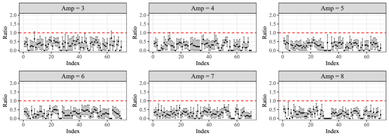
Figure 1: Realized ratios between $\mathbb{P}(\Pi_{j}\geq 1/2)$ and $\mathbb{E}[\Pi_{j}]$, along with $95\%$ confidence intervals, estimated from $1,000$ repetitions. The setting is that from Figure 5. We caution the reader when interpreting the reported values of the ratios since there is a multiple selection issue at play here. The largest observed ratios indicate that the means are larger but also that the difference between the empirical means and the true means may also be large. To drive this point home, suppose we are to look at $m$ random variables all with means less than 0.8, say. Suppose each empirical mean has a standard deviation equal to 0.1. Then we would expect to see a few empirical means above 1 even though all theoretical means are below 0.8.

Proposition 1.

1. Assume the pmf of $\Pi_{j}$ is monotonically non-increasing for each $j\in{\mathcal{H}}_{0}$, then condition (6) holds with $\gamma$ being the optimal value of the following linear program (LP):

   $$\begin{array}[]{ll}\text{\em maximize}&\quad\sum_{m\geq M\eta}\,\,y_{m}\\ \text{\em subject to}&\quad y_{m}\geq 0,\\ &\quad y_{m-1}\geq y_{m},~{}m\in[M],\\ &\quad\sum^{M}_{m=0}y_{m}\,m/M=1.\end{array}$$ (10)

2. Assume that for any $j\in{\mathcal{H}}_{0}$,

   $$\int^{\eta}_{0}\mathbb{P}(\Pi_{j}\in[\eta-u,\eta))\mathrm{d}u\geq\int^{\eta-1/M}_{0}\mathbb{P}(\Pi_{j}\in[\eta,\eta+u))\mathrm{d}u,$$ (11)

   then condition (6) holds with $\gamma$ being the optimal value of the following linear program:

   $$\begin{array}[]{ll}\text{\em maximize}&\quad\sum_{m\geq M\eta}y_{m}\\ \text{\em subject to}&\quad y_{m}\geq 0,~{}m\in\{0,1,2,\ldots,M\},\\ &\quad\sum_{m=0}^{M}y_{m}\,\,{m}/{M}=1,\\ &\quad\sum_{m=0}^{M}y_{m}\geq 2,\\ &\quad\sum^{{\left\lceil{\eta M}\right\rceil}-1}_{m=1}my_{m}\geq\sum^{{\left\lfloor{2\eta M-1}\right\rfloor}-{\left\lceil{\eta M}\right\rceil}}_{m=0}\left(2\eta M-1-{\left\lceil{\eta M}\right\rceil}-m\right)y_{{\left\lceil{\eta M}\right\rceil}+m}.\end{array}$$ (12)

3. As a special case of (b), assume that for any $j\in{\mathcal{H}}_{0}$, the pmf of $\Pi_{j}$ is unimodal where the mode is less than or equal to $\eta$ and $\mathbb{P}(\Pi_{j}=0)\geq\mathbb{P}(\Pi_{j}={\left\lceil{\eta M}\right\rceil}/M)$. Then (11) holds and, therefore, (6) holds with $\gamma$ being the optimal value of (12).

4. Suppose there exists a constant $\beta\in[0,1]$ such that for any $j\in{\mathcal{H}}_{0}$, the pmf of $\Pi_{j}$ satisfies

   $$\mathbb{P}(\Pi_{j}=m/M)\leq\beta\cdot\mathbb{P}(\Pi_{j}=(m-1)/M),\qquad\text{for }m\in[M].$$ (13)

   Then condition (6) holds with $\gamma$ being the optimal value of the LP,

   $$\begin{array}[]{ll}\text{\em maximize}&\quad\sum_{m\geq M\eta}\,\,y_{m}\\ \text{\em subject to}&\quad y_{m}\geq 0,\\ &\quad\beta y_{m-1}\geq y_{m},~{}m\in[M],\\ &\quad\sum^{M}_{m=0}y_{m}\,m/M=1.\end{array}$$ (14)

For illustration, Figure 3 plots the optimal value of (10) versus $M$ with $\eta=0.501$, $0.751$ and $1$, respectively. Taking $M=31$ and $\eta=0.501$ for example, we see that (6) holds with $\gamma=1$. Also, and this is important for later, (6) holds with $\gamma=1$ for $M=31$, $\eta=1/2$.

The proof of Proposition 1 is deferred to Appendix B.1 and we pause here to parse the claims. The monotonicity assumption in part (a) states that the chance that a null variable gets selected 50 times is at most that it gets selected 49 times, which is at most that it gets selected 48 times and so on. (When we say chance, recall that the probability is taken over $\bm{X},\bm{Y},\widetilde{\bm{X}}^{1},\ldots,\widetilde{\bm{X}}^{M}$.) In part (b), (11) is a relaxed version of the monotonicity condition. To be sure, if the pmf of $\Pi_{j}$ is monotonically non-increasing, then (11) holds. Setting $F_{-}(x):=\mathbb{P}(X<x)$, condition (11) says this: the area between the two curves $y=F_{-}(x)$ and $y=F_{-}(\eta)$ (the latter does not vary with $x$) over the interval $[0,\eta]$—the blue area in Figure 2—is larger than the area between the same two curved curves over $[\eta,2\eta-1/M]$—the red area in Figure 2. In other words, the pmf of $\Pi_{j}$ is skewed towards the left as illustrated in Figure 2(b). Part (d) shows that we can sharpen the bound (as illustrated in Figure 4) if the pmf of $\Pi_{j}$ decays at a faster rate—$\mathbb{P}(\Pi_{j}=m/M)\leq\beta\mathbb{P}(\Pi_{j}=(m-1)/M)$—where the smaller $\beta$, the faster the decay. In this paper, we only consider $\beta=1$ (the weakest possible condition), which just says that the pmf is monotonically non-increasing.

(a) $F_{-}(x)=\mathbb{P}(X<x)$.

(b) Probability mass function.

Figure 2: An example of a distribution obeying (11).

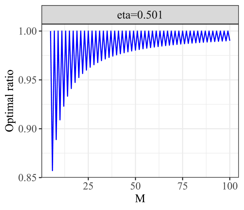
(a) $\eta=0.501$

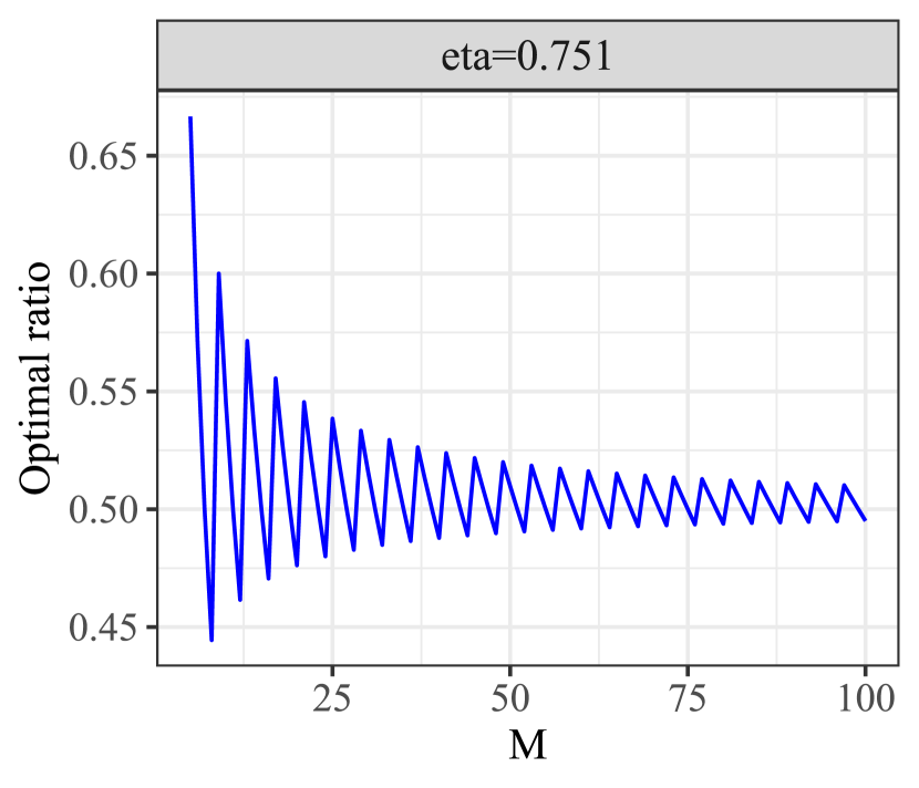
(b) $\eta=0.751$

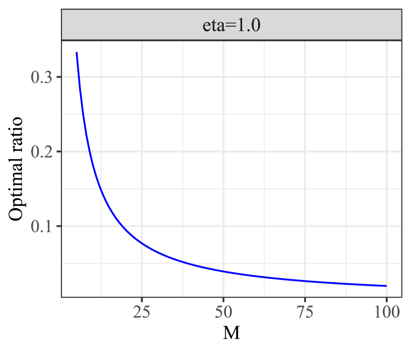
(c) $\eta=1$

Figure 3: Optimal value of (10) as a function of the number $M$ of replicates.

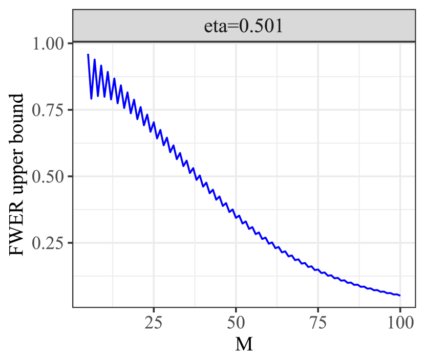
(a) $\eta=0.501$

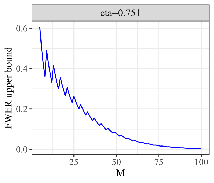
(b) $\eta=0.751$

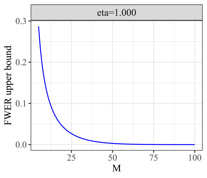
(c) $\eta=1$

Figure 4: Optimal value of (14), with $\beta=0.9$, as a function of the number $M$ of replicates.

3.2 Numerical evaluation of the “derandomization” effect

To illustrate the effect of “derandomization”, we compare derandomized knockoffs with vanilla knockoffs in a small-scale and a large-scale simulation study. Our method is implemented in the R derandomKnock package, available at https://github.com/zhimeir/derandomKnock; code to reproduce all the numerical results from this paper can be found at https://github.com/zhimeir/derandomized_knockoffs_paper. We evaluate the difference in the type-I error, the power and the stability of the selection set. Throughout this section, we set $\eta=0.5$ and $M=31$, which according to Proposition 1 yields $\mathbb{E}[V]\leq v$ (recall that $v$ is the nominal level of the base procedure) under the monotonicity assumption. Here, $Y$ is generated from a linear model conditional on the feature vector $X$, namely,

$$Y\mid X_{1},\ldots,X_{p}\sim\mathcal{N}(\beta_{1}X_{1}+\ldots+\beta_{p}X_{p},1).$$ (15)

As for the covariates, $X$ is drawn from a multivariate Gaussian distribution with parameters to be specified below. We remark that under this model, testing conditional independence is the same as testing whether $\beta_{j}=0$.

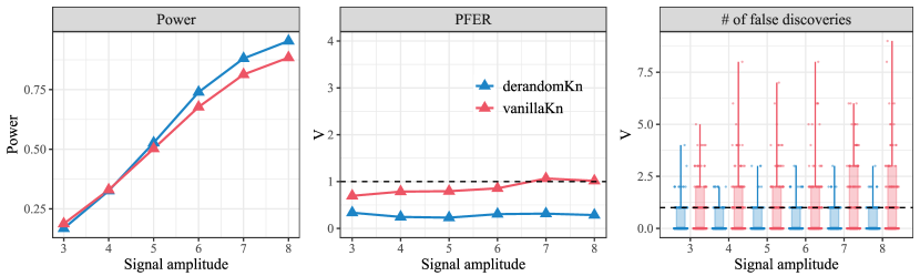
Figure 5: Performance of derandomized and vanilla knockoffs in the small-scale study. Here, $n=200$, $p=100$, $X\sim{\mathcal{N}}(\bm{0},\bm{\Sigma})$ with $\Sigma_{ij}=0.6^{|i-j|}$, and $Y\mid X$ is generated from a linear model with $30$ non-zero coefficients. Each nonzero coefficient $\beta_{j}$ takes value $\pm A/\sqrt{n}$ where the signal amplitude $A$ ranges in $\{3,4,\ldots,8\}$ and the sign is determined by i.i.d. coin flips. The locations of the non-zero signal are randomly chosen from $[p]$. We show the averaged results over 200 trials. The parameter $\bm{\beta}$ is fixed across trials so that the distribution of $(X,Y)$ does not vary. The dashed black line indicates the target PFER level $v=1$. In the boxplot, the box is drawn from the $10$th quantile to the $90$th quantile; the whiskers represent the maximum and the minimum of the data; each jittered dot represents a raw data points outside of the $[10,90]$th percentile range.

Figure 5 compares the performance of derandomized and vanilla knockoffs in the small-scale study. The construction of knockoffs in this study is based on a version suggested by Spector and Janson, (2020), and we use the LCD statistic to tease the signal and noise apart. We can see that both procedures control the PFER, while the power of derandomized knockoffs is slightly better than that of vanilla knockoffs. The boxplot shows that derandomization significantly decreases the marginal selection variability as claimed earlier (we additionally provide the frequencies of the number of false discoveries resulting from both methods in Table 3 in Appendix D.3).

PFER control is theoretically guaranteed with our parameter choices since the ratio between $\mathbb{P}(\Pi_{j}\geq 1/2)$ and $\mathbb{E}[\Pi_{j}]$ is below one for all null variables $j$, as seen earlier in Figure 1. A different way to establish validity is to check the monotonicity condition from Proposition 1 (which in turn implies that none of the ratios exceed one). Figure 6 shows the pooled histograms of all (nonzero) null $\Pi_{j}$’s; the non-increasing property of the pooled distributions is clear.

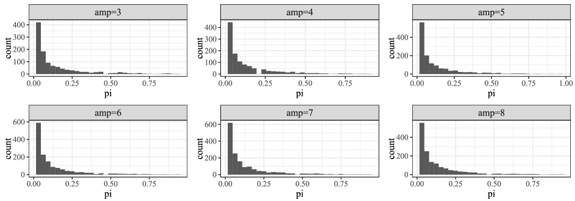
Figure 6: Pooled histograms of all nonzero null $\Pi_{j}$’s under different signal amplitude. The experiment setting is the same as in Figure 5.

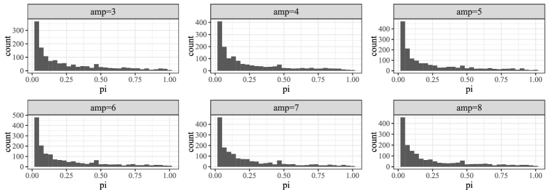
Figure 29: Pooled histograms of all nonzero null $\Pi_{j}$’s for different signal amplitudes. The experiment setting is the same as in Figure 7.

Our large-scale study uses the same LCD statistic and $M=31$, with the knockoff construction based on the version described in Candès et al., (2018). As shown in Figure 7, we observe similar results: both derandomized and vanilla knockoffs control the PFER as expected; the power of derandomized knockoffs is slightly higher than that of the vanilla knockoffs; and derandomized knockoffs has a lower marginal variability than vanilla knockoffs. In addition, the frequencies of the number of false discoveries $V$ are recorded in Table 4 for both methods respectively; the pooled histograms of all null $\Pi_{j}$’s are constructed in Figure 29 and we refer the readers to Appendix D.2 for other diagnostic plots.

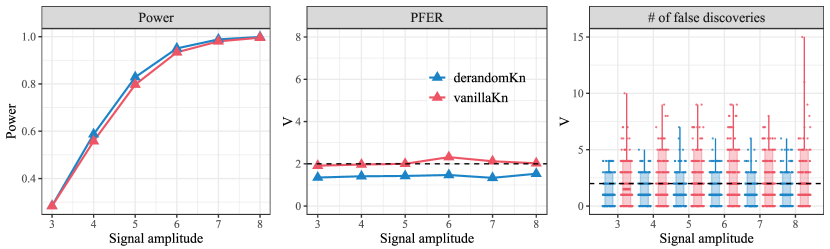
Figure 7: Performance of derandomized and vanilla knockoffs in the large-scale setting. Here, $n=2000$, $p=1000$ and $\Sigma_{ij}=0.5^{|i-j|}$. $Y\mid X$ is generated from a linear model with $60$ non-zero coefficients. The experiment settings are otherwise the same as in Figure 5. The dashed black line corresponds to the target PFER level $v=2$. The construction of boxplots is as in Figure 5.

3.3 Improving assumption-free guarantees

We are primarily interested in a relatively large number $M$ of repetitions in order to enable stable decision making. In the case where $M$ is low, it is possible to significantly improve on the assumption-free bound $\mathbb{E}[V]~{}\leq~{}v/\eta$. Indeed, assuming that the knockoff features are conditionally i.i.d., then the number of selections $M\Pi_{j}$ is binomial conditional on $\bm{X}$ and $\bm{Y}$, i.e. $M\Pi_{j}|\bm{X},\bm{Y}\sim\operatorname{Bin}(M,\mathbb{P}(j\in\hat{{\mathcal{S}}}^{1}\mid\bm{X},\bm{Y}))$. Therefore, the PFER can be directly computed via

$$\mathbb{E}[V]=\mathbb{E}\left[\sum_{j\in{\mathcal{H}}_{0}}\mathbb{P}(j\in\hat{{\mathcal{S}}}\mid\bm{X},\bm{Y})\right] =\mathbb{E}\left[\sum_{j\in{\mathcal{H}}_{0}}\mathbb{P}(M\Pi_{j}\geq M\eta\mid\bm{X},\bm{Y})\right].$$

For example, let us consider the case $\eta=0.5$ and $M=3$. Setting $p_{j}:=\mathbb{P}(j\in\hat{{\mathcal{S}}}^{1}\mid\bm{X},\bm{Y})$ gives

$$\mathbb{E}[V] =\mathbb{E}\left[\sum_{j\in{\mathcal{H}}_{0}}p^{3}_{j}+3p_{j}^{2}(1-p_{j})\right]=\mathbb{E}\left[\sum_{j\in{\mathcal{H}}_{0}}p_{j}\left(p_{j}^{2}+3p_{j}(1-p_{j})\right)\right]\leq 1.125v,$$

where the last inequality follows from two facts, namely,

$$\max_{x\in[0,1]}(x^{2}+3x(1-x))=1.125~{}\text{ and }~{}\sum_{j\in{\mathcal{H}}_{0}}\mathbb{P}(j\in\hat{{\mathcal{S}}}^{1})\leq v.$$ (16)

This bound is of course better than $\mathbb{E}[V]\leq 2v$ from (8). Such calculations for any value of $\eta$ and $M$ provide a tighter control and can be carried out in a completely offline fashion. In this spirit, Figure 8 shows a valid assumption-free bound for a number of repetitions ranging from $2$ to $50$.

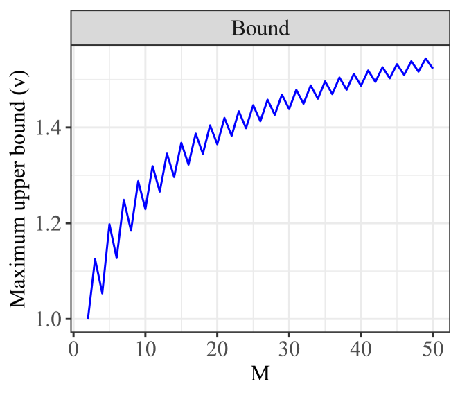
Figure 8: (a) Refined assumption-free PFER bounds as a function of the number of repetitions. The PFER bound is the number reported on the y-axis times the PFER of the base procedure. (b) Value of $p_{j}$ at which the upper bound as in (16) (shown for $M=3$) is achieved.

4 Theoretical guarantees: controlling the $k$-FWER

Another widely used type-I error measure is the $k$ family-wise error rate ($k$-FWER): defined as the probability of making at least $k$ false discoveries, $k\operatorname{-FWER}=\mathbb{P}(V\geq k)$. Dating back to Bonferroni (Dunn,, 1961) and Holm, (1979), many procedures guaranteeing $k\operatorname{-FWER}$ control have been proposed. Most operate on p-values and many require various assumptions on the dependence structure between these p-values (see, e.g. Karlin and Rinott, (1980); Hochberg, (1988); Benjamini and Yekutieli, (2001); Romano et al., (2010)). We refer the readers to Guo et al., (2014); Duan et al., (2020) and the references therein for a survey of these methods.

We now demonstrate how to tune the parameters for derandomized knockoffs to control the $k\operatorname{-FWER}$. Our exposition parallels that from the previous section.

Theorem 2.

Let $V$ be the number of false discoveries after applying derandomized knockoffs (Algorithm 1) with a base procedure obeying $\text{PFER}\leq v$. Suppose condition (6) holds and that for each $k\geq 1$,

$$\mathbb{P}(V\geq k)~{}\leq~{}\dfrac{\rho\mathbb{E}[V]}{k}.$$ (17)

Then the $k\operatorname{-FWER}$ is controlled via

$$\mathbb{P}(V\geq k)~{}\leq~{}\dfrac{\rho\gamma v}{k}.$$ (18)

In particular, by Markov’s inequality one always has $\rho=1$, and consequently,

$$\mathbb{P}(V\geq k)~{}\leq~{}\gamma v/k.$$

The proof of this result is straightforward since we have

$$\mathbb{P}(V\geq k)\leq\dfrac{\rho\mathbb{E}[V]}{k}\leq\dfrac{\rho\gamma v}{k},$$

where the last inequality follows from Theorem 1.

Set $h(x):=x$ and let $Z\sim\mathrm{NB}(v,1/2)$, where $\mathrm{NB}(m,q)$ denotes a negative binomial random variable, which counts the number of successes before the $m$-th failure in a sequence of independent Bernoulli trials with success probability $q$. With this, the right-hand side of (18) can be expressed as $\rho\gamma\mathbb{E}[h(Z)]/k$ (by simply observing that $\mathbb{E}[Z]=v$). This leads to the following extension:

Corollary 1.

Let $h:\mathbb{R}\mapsto\mathbb{R}$ be a convex, non-negative and non-decreasing function. In the setting of Theorem 2, suppose that

$$\mathbb{P}(V\geq k)\leq\dfrac{\rho\mathbb{E}[h(V)]}{h(k)}.$$ (19)

Then the $k\operatorname{-FWER}$ obeys

$$\mathbb{P}(V\geq k)\leq\dfrac{\rho\mathbb{E}[h(Z/\eta)]}{h(k)},\qquad Z\sim\mathrm{NB}(v,1/2).$$ (20)

In particular, Markov’s inequality shows that (20) always holds with $\rho=1$.

The proof of Corollary 1 is deferred to Appendix B.2.

4.1 Guarantees under mild assumptions

While (17) holds with $\rho=1$, we observe in simulations that this value is often quite conservative and we give an example where (17) holds with $\rho=1/2$. The proof and an extension of the proposition below are given in Appendix B.3.

Proposition 2.

In the setting of Theorem 2, suppose the pmf of $V$ is skewed to the left of $k$ in the sense that

$$\sum_{u=1}^{k-1}\,\mathbb{P}(V\in[k-u,k))~{}\geq~{}\sum_{u=1}^{k}\,\mathbb{P}(V\in[k,k+u))$$ (21)

(observe the similarity with (11)). Then condition (17) holds with $\rho=1/2$.

In applications, $k$ and $\alpha$ are supplied and we provide below some guidance on the selection of $v$ and $\eta$ to control the $k$-FWER at level $\alpha$. In order to do so, however, we must extend the base procedure to control the PFER at levels $v$ which may not be integer valued.

Non-integer $v$

Let ${\left\lfloor{v}\right\rfloor}$ be the integer part of $v$ and sample a random variable $U\sim\mathrm{Bern}(v-{\left\lfloor{v}\right\rfloor})$. If $U=1$, run the $({\left\lfloor{v}\right\rfloor}+1)$-knockoffs and ${\left\lfloor{v}\right\rfloor}$-knockoffs otherwise. It is easy to see that such an algorithm controls the PFER at level $v$.

Choices of parameters for larger values of $k$

When $k\geq\max(1/(4\alpha),2)$, we shall fix $\eta$ to be $0.5$ and choose $M$ such that the optimal value of (10) is one. In this way, all the reported variables are selected at least half of the times by the base procedure. We then set $v=2k\alpha$. For example, when $k=3$ and $\alpha=0.1$, we simply set $v=0.6$ and use the base procedure at level 0.6 as above.

Choice of parameters for smaller values of $k$

In the case where $k=1$ or $k<1/(4\alpha)$, we fix $v=1$. When $k=1$, note that the LHS in (21) vanishes so we cannot make use of this condition. In order to control the FWER at the nominal level $\alpha$, it suffices to control $\gamma$ by $\alpha$ since $\mathbb{P}(V\geq 1)\leq\mathbb{E}[V]\leq\gamma$. As shown in Figure 3, under the monotonicity assumption of each $\Pi_{j}$, pairs $(\eta,M)$ yield different values of $\gamma$. Among those pairs for which $\gamma\leq\alpha$, we shall select the pair with the smallest value of $\eta$. For example, suppose we wish to have $\text{FWER}\leq 0.1$. Then Figure 9(a) plots the admissible pairs $(\eta,M)$ (under the monotonicity condition), among which we shall use $\eta=0.95$ and $M=20$ (one may opt to use a larger value of $M$ to increase stability if the computational cost allows it). Similarly, when $k<1/(4\alpha)$, we cannot use $\eta=0.5$ and $v=2k\alpha$ because such a parameter combination would always yield no selection since $v<\eta$. Figure 9(b) plots the pairs $(\eta,M)$ controlling the $2$-FWER by $0.1$ (once again, under the monotonicity condition). According to this plot, we can pick $\eta=0.81$ and $M$ within the computational limit as large as possible in order to enhance stability. In our simulation, we shall take $M=30$.

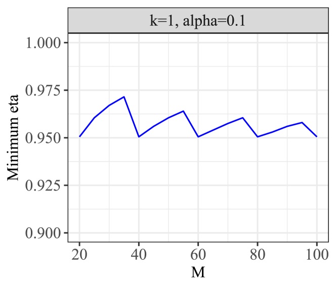
(a) $k=1$ and $\alpha=0.1$.

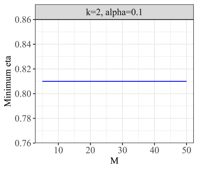
(b) $k=2$ and $\alpha=0.1.$

Figure 9: Pairs $(\eta,M)$ controlling the $k$-FWER control at level $\alpha$ with $v=1$.

4.2 Numerical evaluation of the derandomization effect

We perform two numerical experiments to gauge the performance of derandomized knockoffs. In this study, the response $Y$ is sampled from a logistic model

$$Y\mid X_{1},\ldots,X_{p}\sim\mathrm{Bern}~{}\left(\dfrac{\exp(\beta_{1}X_{1}+\ldots+\beta_{p}X_{p})}{1+\exp(\beta_{1}X_{1}+\ldots+\beta_{p}X_{p})}\right)$$ (22)

and $X$ is drawn from a multivariate Gaussian distribution with parameters to be specified later on. As in Section 3.2, the vector of regression coefficients is sparse so that most of the hypotheses are actually null; under this model, testing conditional independence is the same as testing whether $\beta_{j}=0$.

We evaluate derandomized knockoffs on a small-scale and a large-scale data set. In the small-scale study, the knockoff construction is the same as that from Section 3.2, and the LCD statistic is used as our importance statistic. $M=30$ knockoff copies generated in each run and the selection threshold is $\eta=0.81$. Under the monotonicity constraint, the value of (10) is $0.39$. According to Theorem 2, we thus control the $2$-FWER at level $0.1$. Figure 10 displays the results of the small-scale experiment, where derandomized and vanilla knockoffs obey $\text{$2$-FWER}\leq 0.1$. As before, the boxplot shows that derandomized knockoffs exhibits less marginal randomness than vanilla knockoffs. At the same time, we can clearly see a substantial power gain.

We empirically verify the monotonicity assumption and the skewness property (21) by plotting the histograms of null $\Pi_{j}$’s and false discoveries $V$ respectively in Figure 12 and 13. Under the monotonicity assumption, we expect to see the ratios obeying $\mathbb{P}(\Pi_{j}\geq 0.81)/\mathbb{E}[\Pi_{j}]\leq 0.39$, which is indeed the case as shown in Figure 11.

In the large-scale experiment, the construction of knockoffs and the feature importance statistics are the same as in Section 3.2; the number of knockoff copies is $M=31$ and the selection threshold is $\eta=0.5$ (this yields $\gamma=1$ under the monotonicity constraint). Figure 14 presents the results from which we observe that derandomized knockoffs achieves comparable power, lower $k$-FWER, and reduced variability when compared with vanilla knockoffs. Additionally, we plot the ratios between $\mathbb{P}(\Pi_{j}\geq\eta)$ and $\mathbb{E}[\Pi_{j}]$, histograms of the $\Pi_{j}$’s and the number of false discoveries in Figure 30-32 in Appendix D.2.

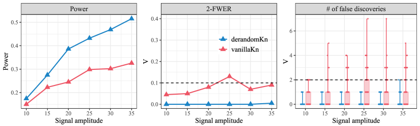
Figure 10: Performance of derandomized knockoffs ($\eta=0.81$ and $v=1$) and vanilla knockoffs. The target $2$-FWER level is $0.1$. In this setting, $n=300$ and $p=50$, $X\sim{\mathcal{N}}(0,\bm{\Sigma})$ with $\Sigma_{ij}=0.5^{|i-j|}$. $Y\mid X$ is sampled from a logistic model (22) with $30$ non-zero entries in $\bm{\beta}$. These nonzero entries take values $\pm A/\sqrt{n}$, where the signal amplitude $A$ ranges in $\{10,15,\ldots,35\}$ and the sign is determined by i.i.d. coin flips. The setting is otherwise the same as in Figure 5. We indicate the target $2$-FWER level $\alpha=0.1$ and $\text{PFER}=2$ with a dashed line. Each point in the first two panels represents an average over $200$ replications. The construction of boxplots is as in Figure 5. Exact frequencies of the number of false discoveries are provided in Table 5, Appendix D.3.

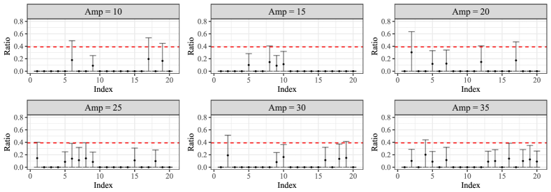
Figure 11: Realized ratios between $\mathbb{P}(\Pi_{j}\geq 0.81)$ and $\mathbb{E}[\Pi_{j}]$ with corresponding $95\%$ confidence intervals estimated from $200$ repetitions. The setting is the same as in Figure 10. The red dashed line corresponds to the target upper bound of $0.39$.

Figure 12: Pooled histograms of all nonzero null $\Pi_{j}$’s. The experiment setting is the same as in Figure 10.

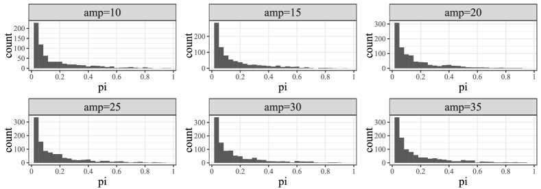
Figure 13: Histograms of the number of false discoveries $V$. The setting is the same as in Figure 10.

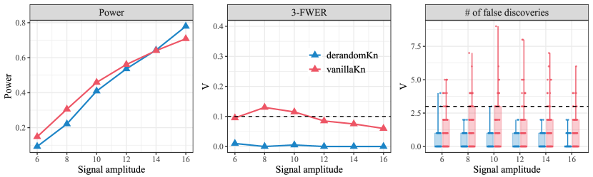
Figure 14: Results from derandomized knockoffs ($\eta=0.5$ and $v=0.6$) and vanilla knockoffs. In this setting, $n=2000$, $p=1000$ and $\Sigma_{ij}=0.2^{|i-j|}$. The number of signals is $60$, and the signal amplitude $A$ ranges in $\{6,8,\ldots,16\}$. The setting is otherwise the same as in Figure 10. We indicate the target 3-FWER level $\alpha=0.1$ and $\text{PFER}=3$ with a dashed line. Each point in the first two panels represents an average over $200$ replications. The construction of boxplots is as in Figure 5.

5 Numerical simulations

Thurs far, we merely demonstrated the enhanced stability of randomized knockoffs when compared to the base procedure. It is, however, unclear whether this stability improvement comes at a price of a potential power loss, as is often seen in the literature on stability selection. This section dispels this concern by comparing our procedure with its competitors via further numerical studies.

5.1 PFER control

In our first experiment, we keep the two simulation settings from Section 3 and compare derandomized knockoffs with a p-value based method applying a Bonferroni correction and with stability selection. The p-values used in the Bonferroni’s procedure are computed from the conditional randomization test (CRT; Candès et al., 2018) in the small-scale study, and from multivariate linear regression in the large-scale study. The CRT p-values are in general more powerful but require intensive computations. This is why we only calculate them in the small-scale study. For stability selection, we use the stabs R-package (Hofner and Hothorn,, 2015) and take the selection threshold to be $0.75$ suggested by the example from the R-package.

Small-scale study

We can see in Figure 15 that all three procedures control the PFER as expected. The power of derandomized knockoffs is slightly better than that of the Bonferroni procedure with CRT p-values. Stability selection suffers a huge power loss vis a vis the other methods due to sample splitting and a conservative choice of threshold.

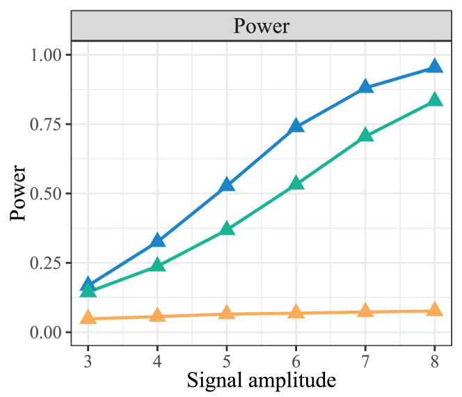
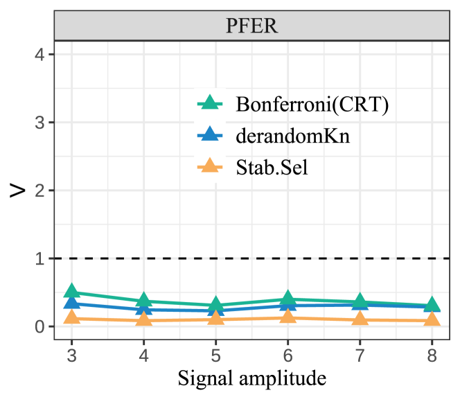
Figure 15: Results from derandomized knockoffs, stability selection and the Bonferroni correction with CRT p-values. The simulation setting is the same as that in Figure 5.

Large-scale study

In this case, we see from Figure 16 that the three procedures control the PFER (up to fluctuations). Derandomized knockoffs has a higher power than the other methods. The Bonferroni correction suffers a power loss because of the low quality of the p-values. Once again, stability selection loses power due to sample splitting and a conservative choice of threshold.

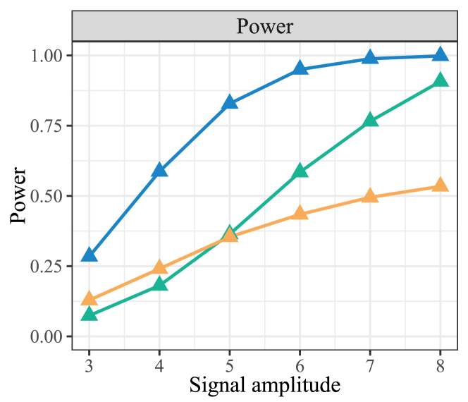
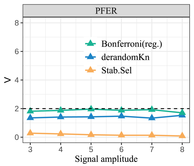
Figure 16: Results from derandomized knockoffs, stability selection and the Bonferroni correction with regression p-values. The simulated setting is the same as that in Figure 7.

5.2 $k$-FWER control

We now turn our attention to evaluating $k$-FWER control, following the set of simulation settings from Section 4. In the small-scale experiment, we compare derandomized knockoffs with stability selection (the implementation is the same as in Section 5.1) and the Bonferroni’s method where the p-values are computed via CRT. In the large-scale experiment, it is computationally very expensive to compute the CRT p-values as observed earlier. How about other p-values? The truth is that p-value based methods face a serious problem since, to the best of our knowledge, it is totally unclear how to compute valid p-values for conditional hypothesis testing; that is, for determining whether $\beta_{j}=0$. The reader may consider that in our high-dimensional logistic regression setting, the maximum likelihood estimator does not even exist. This is the reason why in the large-scale experiment, we forego the comparison with the Bonferroni procedure and only compare with the stability selection procedure (with the same parameters used in the small-scale experiment).

Figure 17 concerns the small-scale study and show the realized power and FWER. Figure 18 displays the same statistics in the large-scale study. As before, we see that both procedures control the FWER. We can also see that derandomized knockoffs yields a much higher power.

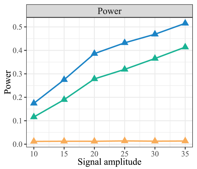
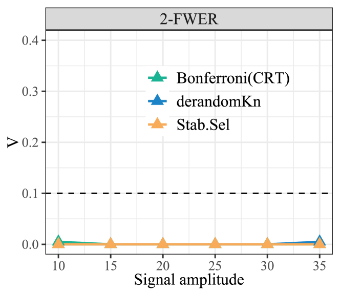
Figure 17: Results from derandomized knockoffs and stability selection. The simulation setting is the same as that in Figure 10.

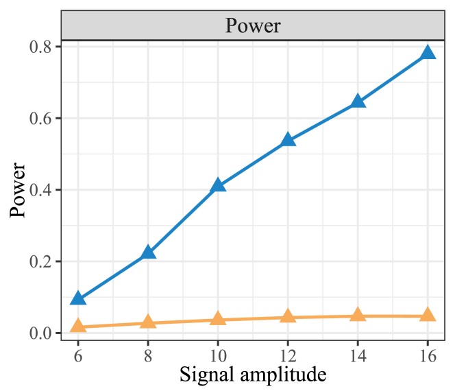
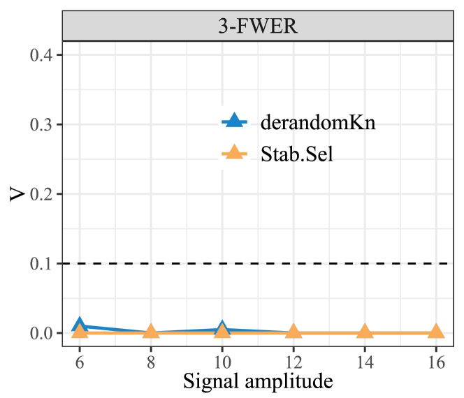
Figure 18: Results from derandomized knockoffs and stability selection. The simulation setting is the same as that in Figure 14.

6 Application to multi-stage GWAS

6.1 Background

The main goal of GWAS is to detect single-nucleotide polymorphisms (SNPs) associated with certain phenotypes. The task is commonly carried out in multiple stages, see e.g., Kote-Jarai et al., (2011); Thomas et al., (2009); Lambert et al., (2013). The purpose of the early stages is often exploratory so that researchers tend to consider more liberal type-I error criteria (such as FDR) to allow for the inclusion of more candidates. The end-stage study is, in contrast, confirmatory, thus asking for a more stringent type-I error criterion (such as FWER). Informally, we can say that the early stage study narrows down the choices to a subset of “candidate SNPs”, whereas the end-stage study pins down the final discoveries. Figure 19 provides a pictorial description of a typical multi-stage GWAS workflow. Here, we would like to apply derandomized knockoffs to the end stage, paving the way to reliable and stable decision making.

Figure 19: A typical workflow of multi-stage GWAS.

6.2 Answering the same question in stages

We pause to discuss challenges associated with multi-stage studies. Although our methods apply regardless of the relationship between a phenotype $Y$ and genetic variants $X_{1},\ldots,X_{p}$, and always yield type-I error control, it may simplify the discussion to consider a standard linear model relating the quantitative $Y$ to $X$ to bring the reader onto familiar grounds (recall this is purely hypothetical). Consider a geneticist who has genotyped a number of sites. She wants to know whether the coefficient $\beta_{j}$ associated with the variant $X_{j}$ vanishes or not. Suppose now that in a first stage—e.g. after analyzing the results of a first study—she thins out the list of possibly interesting variants, those for which she suspects $\beta_{j}$ may not be zero. In a later confirmatory study, we want her to determine whether the coefficients of the screened variables in a model that still includes all the variants $X_{1},\ldots,X_{p}$ she was originally interested vanish or not. It might be tempting to test in the second stage whether coefficients vanish in the reduced model only including those variables that passed screening. However, note that this would lead to test hypotheses that are different from those we started with, not merely a subset of them. To bring this point home, imagine that only one variable passed screening. Then in the second stage, this strategy would lead to test a marginal test of hypothesis, which is not what our geneticist wants (she wants a conditional test). This change of hypotheses so strongly influenced by the random results of the selection of the first stage seems hardly coherent with the goal of the scientific study. (For more discussion about full versus reduced model inference, we refer the reader to Wu et al., (2010); Wasserman and Roeder, (2009); Barber et al., (2019) and Fan and Lv, (2008); Voorman et al., (2014); Belloni et al., (2014); Ma, (2017).)

In light of this, this paper proposes a pipeline for multi-stage GWAS that answers the same question throughout the stages. More specifically, from the very first stage, we are committed to testing the conditional independence hypothesis:

$${\mathcal{H}}_{j}:~{}Y~{}\rotatebox[origin={c}]{90.0}{$\models$}~{}X_{j}\mid X_{-j},$$

where $X_{-j}$ corresponds to all the SNPs except $X_{j}$. This means that if ${\mathcal{C}}$ is the candidate set selected by previous stages, we test ${\mathcal{H}}_{j}$ for each $j\in{\mathcal{C}}$ in the end stage. We do this by applying derandomized knockoffs, which controls type-I errors regardless of the procedures used in the previous stages. This is very different from existing approaches which switch the inferential target and would test whether a variable $j\in{\mathcal{C}}$ is significant in a model that only includes variables in ${\mathcal{C}}$ (Lee et al.,, 2013; Tibshirani et al.,, 2016; Tian et al.,, 2018; Fithian et al.,, 2014; Barber et al.,, 2019).

6.3 A synthetic example with real genetic covariates

We now rehearse the pipeline for multi-stage GWAS and showcase the performance of derandomized knockoffs using a synthetic example with real genetic covariates. Recall that the key assumption underlying the knockoffs procedure is the knowledge of the distribution of $X$. For real data analysis, the distribution of $X$ can only be approximated, which raises the concern of whether such an approximation invalidates FWER control. With this in mind, we set up a simulation with real covariates and synthetic phenotypes generated from a known model. The knockoffs are constructed with the approximated distribution of $X$ and we verify whether or not FWER is controlled at the desired level since we know the true conditional model. (Recall that FWER constrol does not in any away depend upon the unknown relationship between $Y$ and $X$.)

Data acquisition

We obtain the covariate matrices by subsetting the genoypte matrix from the UK Biobank data set (Bycroft et al.,, 2018), where we only include the $9{,}537$ SNPs from chromosome $22$. A subset of $n=6,000$ samples is drawn for the early-stage GWAS and $20$ other disjoint subsamples (each of size $n=3{,}000$) for the end-stage GWAS (see Figure 20 for illustration), where all samples are unrelated British individuals. The FWER and power reported are averaged over these $20$ independent subsets. Conditional on $X$, the variable $Y$ is generated from a linear model:

$$Y\mid X_{1},\ldots,X_{p}\sim\mathcal{N}(\beta_{1}X_{1}+\ldots+\beta_{p}X_{p},1).$$ (23)

The $40$ non-null features are equally divided into $20$ clusters, where the clusters are evenly spaced on the chromosome. The magnitudes and signs of the coefficients vary across clusters, and are the same within each cluster. The relative absolute values of the magnitudes are chosen uniformly at random so that the ratio between the smallest and the largest is $1/19$; the signs of the coefficients are determined by independent coin flips. The heritability, defined as $h^{2}:=\operatorname{Var}(X^{\top}\beta)/\operatorname{Var}(Y)$, is used as a control parameter; informally, this is the fraction of the variance of the phenotype explained by genetic factors.

Figure 20: Splitting the UK Biobank data set and obtaining covariate matrices.

Pre-processing and clustering

We follow the pre-processing steps in Sesia et al., 2020b , and only consider the biallelic SNPs with minor allele frequency above $0.1\%$ and in Hardy-Weinberg equilibrium ($10^{−6}$). A typical challenge in GWAS is the presence of linkage disequilibrium, which makes it essentially difficult to pin-point the important SNPs. To address this difficulty, we use the treatment suggested in Sesia et al., 2020b and partition the genetic variants into groups—we shall use the words “groups” and “clusters” interchangeably—via adjacency-constrained hierarchical clustering. After clustering, we treat the clusters as the inferential object and test whether or not a cluster of SNPs is independent of the phenotype conditional on all other clusters of SNPs. Formally, let $G$ be a partition of $[p]$. For each cluster $g\in G$, the hypothesis to be tested is

$${\mathcal{H}}_{g}:~{}Y~{}\rotatebox[origin={c}]{90.0}{$\models$}~{}X_{g}\mid X_{-g}.$$ (24)

For example, suppose as in Figure 21 that we have $12$ SNPs divided into four clusters. With $g=\{5,6\}$, hypothesis (24) translates into $(X_{5},X_{6})~{}\rotatebox[origin={c}]{90.0}{$\models$}~{}Y\mid X_{-\{5,6\}}$. The sizes of the clusters determine how fine our discoveries are. In the experiment we consider five levels of resolution: $2\%$, $10\%$, $20\%$, $50\%$ and $100\%$, where the resolution is defined as the number of groups divided by the number of SNPs.

Figure 21: Visual illustration of the partition of SNPs.

Early-stage GWAS

We apply two procedures to identify candidate hypotheses:

1. The first is the group model-X knockoffs procedure (Sesia et al., 2020b, ) with FDR controlled at level $0.5$. The selected clusters then become the candidate SNP clusters for the end stage.

2. The second is motivated by the practice of early-stage studies, which often only provide summary statistics such as p-values and, lead to the selection of candidate SNPs via p-value cutoffs. To evaluate the performance of derandomized knockoffs in such a context, we screen candidate SNPs as follows: compute a marginal regression p-value for each SNP and select those SNPs with a p-value below $5\times 10^{-6}~{}(\approx 0.05/p)$. Then a SNP cluster is considered a “candidate” if at least one of its SNPs passes the p-value threshold.

Figure 22 summarizes the basic steps of our hypothetical multi-stage GWAS.

Figure 22: Schematic representation of the multi-stage GWAS used in the numerical study.

Knockoffs and feature importance statistics construction

Let ${\mathcal{G}}$ be the set of candidate SNP clusters identified during the earlier stage. We proceed to construct a conditional knockoff copy only for $X_{{\mathcal{G}}}$: the knockoff copy ${\widetilde{X}}_{{\mathcal{G}}}$ satisfies the knockoff properties conditional on $X_{-{\mathcal{G}}}$; that is, ${\widetilde{X}}_{{\mathcal{G}}}~{}\rotatebox[origin={c}]{90.0}{$\models$}~{}Y\mid(X_{{\mathcal{G}}},X_{-{\mathcal{G}}})$ and

$$(X_{{\mathcal{G}}},{\widetilde{X}}_{{\mathcal{G}}})_{\text{swap}(g)}|X_{-{\mathcal{G}}}\stackrel{{\scriptstyle\mathrm{d}}}{{=}}(X_{{\mathcal{G}}},{\widetilde{X}}_{{\mathcal{G}}})|X_{-{\mathcal{G}}},$$ (25)

where $g$ denotes a SNP cluster that belongs to ${\mathcal{G}}$. Above, $(X_{{\mathcal{G}}},{\widetilde{X}}_{{\mathcal{G}}})_{\text{swap}(g)}$ is obtained from $(X_{{\mathcal{G}}},{\widetilde{X}}_{{\mathcal{G}}})$ by swapping the features $X_{j}$ and ${\widetilde{X}}_{j}$ for each SNP $j\in g$. We model the distribution of $X$ via a hidden Markov model (HMM), and construct (group) HMM knockoffs based on a variant of an existing procedure (Sesia et al.,, 2019; Sesia et al., 2020b, ). The HMM used here describes the distribution of SNPs in unrelated British individuals (Sesia et al., 2020b, ). Details about the construction of ${\widetilde{X}}_{\mathcal{G}}$ are deferred to Appendix D.1. As for the feature importance statistic, we use the (group) LCD statistics introduced in Sesia et al., 2020b .

Results

Figure 23 presents the marginal p-values for a subset of SNPs in the form of a Manhattan plot, where it is easily seen that the selected SNPs are clustered together. Figure 25 shows the realized power, end-stage power (the number of true discoveries divided by the number of non-nulls selected by pre-GWAS) and FWER with different resolutions in the case where the screening step thresholds marginal p-values. Figure 25 presents the same statistics in the case where the screening step uses knockoffs. In both cases, it can readily be observed that even with an approximate distribution of $X$, our procedure successfully controls the FWER. Furthermore, while the candidates selected by p-value thresholding are clustered together (which potentially affects power), the two-stage procedure still makes a reasonable number of findings.

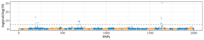
Figure 23: The Manhattan plot of a subset of $2000$ SNPs in the synthetic example. The colors correspond to the clusters at 2% resolution.

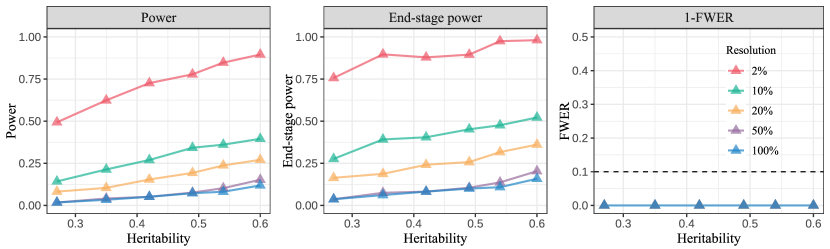
Figure 24: Realized power (left), end-stage power (middle) and FWER (right) in the synthetic multi-stage GWAS. The early-stage GWAS selects SNPs with p-values less than $5\times 10^{-6}$. The target FWER level of derandomized knockoffs is $0.1$.

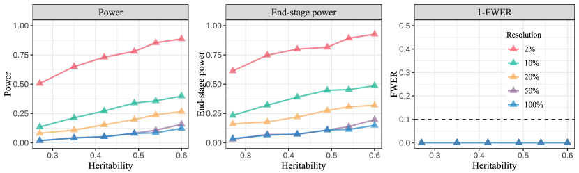
Figure 25: Realized power (left), end-stage power (middle) and FWER (right) in the synthetic multi-stage GWAS. The early-stage GWAS uses model-X knockoffs with target FDR level $0.5$. The target FWER level of derandomized knockoffs is $0.1$.

6.4 End-stage GWAS of prostate cancer

We finally apply our procedure to an end-stage GWAS of prostate cancer. We take the meta-analysis conducted by Schumacher et al., (2018) as the early-stage study, and apply derandomized knockoffs on a data set from UK Biobank for a confirmatory analysis. The UK biobank data set contains genetic information on $161$K unrelated British male individuals and their disease status, i.e., whether or not a participant has reported being diagnosed with prostate cancer.

After selecting p-values from Schumacher et al., (2018) below $10^{-3}$, we end up with $4072$ pre-selected SNPs. (The set of SNPs recorded in Schumacher et al., (2018) can be different from that in the UK Biobank data set. Here, we only consider the intersection of the two sets.)

As in our earlier numerical study, the next step is to partition a priori all the SNPs into clusters at a level of resolution $2\%$. The resulting average length of the clusters is $0.226$ Mb. A cluster is called a candidate cluster if at least one of its SNPs is a candidate SNP. Ten runs of conditional group HMM knockoffs are constructed for the candidate clusters. We compute the group LCD statistics as in the synthetic example from Section 6.3. Six additional covariates, namely, age and the top five principal components of the genotypes are included in the knockoffs predictive model as follows: instead of using the phenotypes as the response, we use the residuals of the phenotypes after regressing out these six additional covariates. The inclusion of these covariates allows us to account for the (remaining) population structure in the data, which increases the detection power. Finally, we apply derandomized knockoffs with target FWER level $0.1$. Table 1 provides detailed information on the final list of clusters when the resolution is $2\%$.

We compare our findings with those from the existing literature. Since our discoveries are SNP clusters and different studies may contain different sets of SNPs, we cannot directly compare the results across different studies. Here we consider findings to be confirmed by another study if the latter reports a SNP whose position is within the genomic locus spanned by a cluster we discovered. With this, it turns out that all of our $8$ findings are confirmed by other studies. Further, $7$ matches are exact in the sense that the leading SNP of a discovered cluster is reported significant in the literature. Specifically, clusters represented by rs12621278, rs1512268, rs6983267, rs7121039, rs10896449 and rs1859962 are replicated by Wang et al., (2015), which is a large GWAS conducted in the Asian population; rs1016343 is confirmed by Hui et al., (2014)—a study specifically investigating the associations of six SNPs including rs1016343 in a Chinese population; the association between rs7501939 and prostate cancer is in Elliott et al., (2010), which is a study focusing on the association of two SNPs including rs7501939 with several diseases.

What would happen if we were a little more liberal? To find out, we also run the derandomized knockoffsset to control the $3$-FWER at level $0.1$: all the SNPs discovered earlier appear in the new discovery set. The more liberal procedure makes seven additional discoveries and the corresponding SNPs are listed in Table 2.

Lead SNP	Chromosome	Position range (Mb)	Size	Confirmed by?
rs12621278	2	173.28-173.58	68	Wang et al., (2015)
rs1512268	8	23.39-23.55	48	Wang et al., (2015)
rs1016343	8	128.07-128.24	45	Hui et al., (2014)
rs6983267	8	128.40-128.47	37	Wang et al., (2015)
rs7121039	11	2.18-2.31	40	Wang et al., (2015)*
rs10896449	11	68.80-69.02	62	Wang et al., (2015)
rs7501939	17	36.05-36.18	55	Elliott et al., (2010)
rs1859962	17	69.07-69.24	40	Wang et al., (2015)

Table 1: Discoveries made by derandomized knockoffs at 2% resolution and the target FWER level set to $0.1$. The asterisk indicates the following: the lead SNP is not found in the literature; however, the literature reports a SNP within the position range of our reported cluster.

Lead SNP	Chromosome	Position range (Mb)	Size	Confirmed by?
rs905938	1	154.80-155.04	66	Wang et al., (2015)*
rs6545977	2	62.81-63.60	65	Wang et al., (2015)*
rs77559646	2	242.07-242.16	35	Kaikkonen et al., (2018)
rs2510769	4	95.28-95.60	59	Wang et al., (2015)*
rs10486567	7	27.56-28.04	87	Haiman et al., (2011)
rs17762878	8	127.85-128.07	70	Wang et al., (2015)*
rs4242382	8	128.47-128.56	34	Zhao et al., (2014)

Table 2: Additional discoveries made by derandomized knockoffs at 2% resolution and the target $3$-FWER level set to $0.1$ (all the SNPs reported in Table 1 is also discovered by this procedure). The setting is otherwise the same as in Table 1.

7 Discussion

We proposed a framework for derandomized knockoffs inspired by stability selection. By exploiting multiple runs of the knockoffs algorithm, our method offers a more stable solution for selecting non-null variables. Leveraging a base procedure with controlled PFER, we show how to achieve PFER and $k\operatorname{-FWER}$ control, these being error metrics perhaps more suitable than FDR for confirmatory stage studies (Tukey,, 1980; Goeman et al.,, 2011) as well as more resource-consuming applications such as end-stage GWAS (Meijer and Goeman,, 2016; Sham and Purcell,, 2014), clinical trials (Crouch et al.,, 2017) and neuro-imaging (Eklund et al.,, 2016). Furthermore, we execute our methodology on a GWAS example and and find that all our findings are confirmed by related studies.

Future work

While the current paper empirically demonstrates enhanced statistical power, it would be of interest to theoretically validate power gains, at least in some simple settings. Also, the machinery described here is general and can be applied to a variety of base procedures—even procedures that do not come with controlled PFER. One would, therefore, ask whether our theoretical framework can be adapted to accommodate such base procedures. Finally, perhaps the most natural question is whether our ideas can be adapted to the more liberal FDR criterion or related error rates such as the false discovery exceedence.

Acknowledgment

The authors would like to thank Malgorzata Bogdan, Lihua Lei, and Chiara Sabatti for helpful discussions. The authors also would like to thank the PRACTICAL consortium, CRUK, BPC3, CAPS, PEGASUS for providing GWAS summary statistics (more information can be found at http://practical.icr.ac.uk/blog/?page_id=8164). Z. R. is supported by the Math + X award from the Simons Foundation, the JHU project 2003514594, the ARO project W911NF-17-1-0304 , the NSF grant DMS 1712800 and the Discovery Innovation Fund for Biomedical Data Sciences. Y. W. is supported partially by the NSF grants CCF 2007911 and DMS 2015447. E. C. is partially supported by NSF via grants DMS 1712800 and DMS 1934578 and by the Office of Naval Research grant N00014-20-12157.

Appendix A More details on $v$-knockoffs

A.1 Algorithm description

Suppose at the $m$-th round, the feature importance statistic $\bm{W}^{m}$ has been computed. The $v$-knockoffs algorithm starts by ordering the features according to the magnitudes of $W^{m}_{j}$, i.e.

$$|W^{m}_{r_{1}}|\geq\ldots\geq|W^{m}_{r_{j}}|\geq\ldots\geq|W^{m}_{r_{p}}|,\qquad\text{for some permutation }~{}r_{1},\ldots,r_{p}.$$

Given a pre-specified integer $v$, the procedure examines the features one by one from $r_{1}$ to $r_{p}$ according to the ordering above until the first time there are $v$ negative $W^{m}_{j}$’s. Formally, the stopping criterion is defined as

$$T_{v}^{m}:=\min\,\Big{\{}k\in[p]\,\mid\,\sum^{k}_{j=1}{\mathbf{1}_{\left\{{W^{m}_{r_{j}}<0}\right\}}}\geq v\Big{\}}.$$

The selected set is then defined to be the collection of the features examined before $T_{v}^{m}$ which have positive signs of feature importance statistics, i.e.,

$$\hat{{\mathcal{S}}}^{m}:=\{r_{j}\,\mid\,j<T_{v}^{m},~{}W^{m}_{r_{j}}>0\}.$$ (26)

Figure 26: Visual illustration of the base procedure.

A.2 Theoretical properties

Lemma 1 (Janson et al., (2016)).

For any integer $v$, the number of false discoveries produced by the $v$-knockoffs procedure

$$V_{m}:=\#\{j\in\mathcal{H}_{0}\cap\hat{{\mathcal{S}}}^{m}\},$$ (27)

is stochastically dominated by a negative binomial variable $\mathrm{NB}(v,1/2)$.

This lemma is originally stated in Janson et al., (2016) for fixed knockoffs in linear models. However, the result is a direct consequence of the coin-flip property (see Candès et al., (2018, Lemma 3.3)); here the coin-flip property means that conditional on $(|W^{m}_{1}|,\ldots,|W^{m}_{p}|)$, the signs of the null $W^{m}_{j}$’s ($j\in\mathcal{H}_{0}$) are i.i.d. coin flips. Therefore, Lemma 1 is also applicable in the model-X setting.

Appendix B Proofs of the main results

B.1 Proof of Proposition 1

Proof of (a)

For every $j\in{\mathcal{H}}_{0}$, the selection probability $\Pi_{j}$ is supported on $\{0,1/M,2/M,\ldots,1\}$. Letting $p_{m}:=\mathbb{P}\left(\Pi_{j}=m/M\right)$ for $m=0,1,\ldots,M$, we can express the ratio as

$$\frac{\mathbb{P}(\Pi_{j}\geq\eta)}{\mathbb{E}[\Pi_{j}]}=\Big{(}\sum_{m\geq\eta M}p_{m}\Big{)}/\Big{(}\sum^{M}_{m=0}p_{m}\cdot\dfrac{m}{M}\Big{)}.$$

By definition, $p_{m}\geq 0$ and $\sum^{M}_{m=0}p_{m}=1$. In addition, by the coin-flip property (see Candès et al., (2018, Lemma 3.3)), $\mathbb{E}[\Pi_{j}]\leq 1/2$ since $j\in{\mathcal{H}}_{0}$, which translates into $\sum^{M}_{m=0}p_{m}\cdot(m/M)\leq 1/2$. Together with the monotonicity assumption, the optimization problem can be written as

$$\begin{array}[]{ll}\text{maximize}&\quad\Big{(}\sum_{m\geq\eta M}p_{m}\Big{)}/\Big{(}\sum^{M}_{m=0}p_{m}\cdot\dfrac{m}{M}\Big{)}\\ \text{subject to}&\quad p_{m}\geq 0,\\ &\quad p_{m-1}\geq p_{m},~{}m\in[M],\\ &\quad\sum^{M}_{m=0}p_{m}=1,~{}\sum^{M}_{m=0}p_{m}\cdot\dfrac{m}{M}\leq 1/2.\end{array}$$ (28)

Setting $y_{m}:=p_{m}/\Big{(}\sum^{M}_{m=0}p_{m}\cdot\dfrac{m}{M}\Big{)}$, optimization problem (28) reduces to

$$\begin{array}[]{ll}\text{maximize}&\quad\sum_{m\geq\eta M}y_{m}\\ \text{subject to}&\quad y_{m}\geq 0,\\ &\quad y_{m-1}\geq y_{m},~{}m\in[M],\\ &\quad\sum^{M}_{m=0}y_{m}\cdot\dfrac{m}{M}=1,\end{array}$$

which proves (a). Here, we use the fact that

$$\sum^{M}_{m=0}p_{m}\cdot\dfrac{m}{M}\leq(\sum^{M}_{m=0}p_{m})\cdot(\frac{1}{M+1}\sum^{M}_{m=0}\frac{m}{M})=\frac{1}{2}$$

holds for any non-increasing sequence $\{p_{m}\}$.

Proof of (b), (c) and (d)

• The proof of (b) is similar except that we replace the monotonicity condition by the condition on the partial summation.

• For (c), note that if the pmf of $\Pi_{j}$ is unimodal where the mode is less than or equal to $\eta$ and $\mathbb{P}(\Pi_{j}=0)\geq\mathbb{P}(\Pi_{j}={\left\lceil{\eta M}\right\rceil}/M)$, then (11) holds.

• The proof of (d) is essentially the same as that of part (a), thus omitting here.

B.2 Proof of Corollary 1

For any monotonically non-decreasing and non-negative function $h:\mathbb{R}\mapsto\mathbb{R}$, Markov’s inequality gives

$$\mathbb{P}(V\geq k) \leq\dfrac{\mathbb{E}[h(V)]}{h(k)}.$$

By the definition of $V$,

$$V=\sum_{j\in{\mathcal{H}}_{0}}\mathbf{1}\{\Pi_{j}\geq\eta\}\leq\sum_{j\in{\mathcal{H}}_{0}}\dfrac{\Pi_{j}}{\eta}=\sum_{j\in{\mathcal{H}}_{0}}\sum_{m=1}^{M}\dfrac{\mathbf{1}\{j\in\hat{{\mathcal{S}}}^{m}\}}{\eta M}=\sum^{M}_{m=1}\dfrac{V_{m}}{\eta M}.$$ (29)

As a consequence,

$$\frac{\mathbb{E}[h(V)]}{h(k)} \stackrel{{\scriptstyle(i)}}{{\leq}}\frac{\mathbb{E}\Big{[}h\left(\sum^{M}_{m=1}V_{m}/\eta M\right)\Big{]}}{h(k)}\stackrel{{\scriptstyle(ii)}}{{\leq}}\sum_{m=1}^{M}\frac{\mathbb{E}[h(V_{m}/\eta)]}{Mh(k)}\stackrel{{\scriptstyle(iii)}}{{=}}\frac{\mathbb{E}[h(V_{1}/\eta)]}{h(k)}.$$

Step (i) holds since $h$ is non-decreasing and $V$ obeys (29); step (ii) follows from the convexity of $h$ and Jensen’s inequality; step (iii) uses the fact that each $V_{m}$ has the same marginal distribution. Putting things together, the $k$-FWER satisfies

$$\mathbb{P}(V\geq k) ~{}\leq~{}\frac{\mathbb{E}[h(V_{1}/\eta)]}{h(k)}.$$

To complete the proof, use the fact that $V_{1}$ is stochastically dominated by $\mathrm{NB}(v,1/2)$ by Lemma 1.

B.3 Proof and extension of Proposition 2

Proof of Proposition 2

The proof of Proposition 2 is a direct consequence of the following result, whose proof is provided in Section C.1.

Lemma 2 (Huber, (2018)).

Let $X$ denote a non-negative random variable. Assume there exists $\xi>0$, such that

$$\int^{\eta}_{0}\mathbb{P}(X\in[\eta-u,\eta))\mathrm{d}u\geq\int^{\xi}_{0}\mathbb{P}(X\in[\eta,\eta+u))\mathrm{d}u,$$

then the following Markovian type tail bound holds:

$$\mathbb{P}(X\geq\eta)\leq\dfrac{\mathbb{E}[X]}{\eta+\xi}.$$

Applying Lemma 2 to the random variable $V$ with $\eta=\xi=k$ completes the proof of Proposition 2.

Extension of Proposition 2

The result below provides conditions under which the bounds in Corollary 1 can be tightened.

Proposition 3.

Consider the setting of Corollary 1.

1. Let $h(x)=x^{\nu}$ for $\nu\geq 1$. Suppose the pmf of $V$ obeys

   $$\sum^{{\left\lfloor{k/\nu}\right\rfloor}-1}_{u=1}\mathbb{P}\left(V\in[k-u,k)\right)+(k/\nu-{\left\lfloor{k/\nu}\right\rfloor})\cdot\mathbb{P}(V\in[k-{\left\lfloor{k/\nu}\right\rfloor},k))\geq\\ \sum^{{\left\lfloor{k/\nu}\right\rfloor}}_{u=1}\mathbb{P}(V\in[k,k+u))+(k/\nu-{\left\lfloor{k/\nu}\right\rfloor})\cdot\mathbb{P}(V\in[k,k+{\left\lfloor{k/\nu}\right\rfloor}+1)),$$ (30)

   then (19) holds with $\rho=1/2$.

2. Let $h(x)=\exp{(\lambda x)}$ for $\lambda\in(0,1]$. Suppose the pmf of $V$ obeys

   $$\sum^{{\left\lfloor{1/\lambda}\right\rfloor}-1}_{u=1}\mathbb{P}\left(V\in[k-u,k)\right)+(1/\lambda-{\left\lfloor{1/\lambda}\right\rfloor})\cdot\mathbb{P}(V\in[k-{\left\lfloor{1/\lambda}\right\rfloor},k))\geq\\ \sum^{{\left\lfloor{1/\lambda}\right\rfloor}}_{u=1}\mathbb{P}(V\in[k,k+u))+(1/\lambda-{\left\lfloor{1/\lambda}\right\rfloor})\cdot\mathbb{P}(V\in[k,k+{\left\lfloor{1/\lambda}\right\rfloor}+1)),$$ (31)

   then (19) holds with $\rho=1/2$.

The proof of Proposition 3 follows from the following lemma, whose proof is provided in Section C.2.

Lemma 3.

Suppose $X$ is a non-negative random variable.

1. If

   $$\int^{\frac{k}{\nu}}_{0}\mathbb{P}(X\in[k-u,k))\mathrm{d}u\geq\int^{\frac{tk}{\nu}}_{0}\mathbb{P}(X\in[k,k+u))\mathrm{d}u$$ (32)

   for some $k,t>0$ and $\nu\geq 1$, then

   $$\mathbb{P}(X\geq k)\leq\dfrac{\mathbb{E}[X^{\nu}]}{(1+t)k^{\nu}}.$$ (33)

2. If

   $$\int^{\frac{1}{\lambda}}_{0}\mathbb{P}(X\in[k-u,k))\mathrm{d}u\geq\int^{\frac{t}{\lambda}}_{0}\mathbb{P}(X\in[k,k+u))\mathrm{d}u$$

   holds for some $k,t,\lambda>0$, then

   $$\mathbb{P}(X\geq k)\leq\dfrac{\mathbb{E}[\exp(\lambda X)]}{(1+t)\exp(\lambda k)}.$$ (34)

Applying Lemma 3 to $V$ with $t=1$ yields Proposition 3.

Appendix C Proofs of auxiliary lemmas

C.1 Proof of Lemma 2

For each $\xi>0$, we introduce an auxiliary random variable $U\sim\text{Unif}[-\xi,\eta]$ independent of $X$. We claim that

$$\mathbb{P}(X\geq\eta)\leq\mathbb{P}(X+U\geq\eta)\leq\dfrac{\mathbb{E}[X]}{\xi+\eta},$$

which completes the proof. To see this, let us start with establishing the second inequality. A direct computation yields

$$\mathbb{P}(X+U\geq\eta) =\mathbb{E}[\mathbb{P}(U\geq\eta-X|X)]$$

$$=\mathbb{E}[\operatorname{\mathds{1}}\{\eta-X\leq-\xi\}]+\mathbb{E}\left[\dfrac{X}{\eta+\xi}\operatorname{\mathds{1}}\{-\xi<\eta-X\leq\eta\}\right]\leq\mathbb{E}\left[\dfrac{X}{\xi+\eta}\right].$$

By definition,

$$\mathbb{P}(X+U\geq\eta) =\dfrac{1}{\eta+\xi}\int^{\eta}_{-\xi}\mathbb{P}(X\geq\eta-u)\mathrm{d}u$$

$$=\dfrac{1}{\eta+\xi}\left[\int^{0}_{-\xi}\mathbb{P}(X\geq\eta-u)\mathrm{d}u+\int^{\eta}_{0}\mathbb{P}(X\geq\eta-u)\mathrm{d}u\right]$$

$$=\dfrac{1}{\eta+\xi}\left[\int^{\eta}_{-\xi}\mathbb{P}(X\geq\eta)\mathrm{d}u-\int^{0}_{-\xi}\mathbb{P}(X\in[\eta,\eta-u))\mathrm{d}u+\int^{\eta}_{0}\mathbb{P}(X\in[\eta-u,\eta))\mathrm{d}u\right]$$

$$=\mathbb{P}(X\geq\eta)+\dfrac{1}{\eta+\xi}\left[-\int^{\xi}_{0}\mathbb{P}(X\in[\eta,\eta+u))\mathrm{d}u+\int^{\eta}_{0}\mathbb{P}(X\in[\eta-u,\eta))\mathrm{d}u\right]$$

$$\geq\mathbb{P}(X\geq\eta),$$

where the last inequality follows from our assumption.

C.2 Proof of Lemma 3

Let $U\sim\text{Unif}[-\frac{tk}{\nu},\frac{k}{\nu}]$ be independent of $X$. We prove that

$$\mathbb{P}(X\geq k)\leq\mathbb{P}(X+U\geq k)\leq\dfrac{\mathbb{E}[X^{\nu}]}{(1+t)k^{\nu}}.$$

The second inequality follows from direct calculations:

$$\mathbb{P}(X+U\geq k) =\mathbb{E}\left[\operatorname{\mathds{1}}\left\{k-X\leq-\frac{tk}{\nu}\right\}\right]+\mathbb{E}\left[\dfrac{\frac{k}{\nu}-k+X}{(1+t)\frac{k}{\nu}}\cdot\operatorname{\mathds{1}}\left\{-\frac{tk}{\nu}<k-X\leq\frac{k}{\nu}\right\}\right]$$

$$\leq\mathbb{E}\left[\dfrac{X-\frac{(\nu-1)k}{\nu}}{(1+t)\frac{k}{\nu}}\right]\leq\dfrac{\mathbb{E}[X^{\nu}]}{(1+t)k^{\nu}},$$

where the last inequality uses $x-\frac{\nu-1}{\nu}k\leq\frac{x^{\nu}}{\nu k^{\nu-1}}$. As for the first inequality,

$$\mathbb{P}(X+U\geq k) =\dfrac{1}{(1+t)\frac{k}{\nu}}\left[\int^{\frac{k}{\nu}}_{-\frac{tk}{\nu}}\mathbb{P}(X\geq k-u)\mathrm{d}u\right]$$

$$=\dfrac{1}{(1+t)\frac{k}{\nu}}\left[\int^{\frac{k}{\nu}}_{-\frac{tk}{\nu}}\mathbb{P}(X\geq k)\mathrm{d}u+\int^{\frac{k}{\nu}}_{0}\mathbb{P}(X\in[k-u,k))\mathrm{d}u-\int^{\frac{tk}{\nu}}_{0}\mathbb{P}(X\in[k,k+u))\mathrm{d}u\right]$$

$$\geq\mathbb{P}(X\geq k)$$

(the last inequality follows from our assumption).

For the second part, introduce an independent uniform random variable $U$ supported on $[-\frac{t}{\lambda},\frac{1}{\lambda}]$. We prove that

$$\mathbb{P}(X\geq k)\leq\mathbb{P}(X+U\geq k)\leq\dfrac{\mathbb{E}[\exp(\lambda X)]}{(1+t)\exp(\lambda k)}.$$

The proof of the first inequality is exactly the same as that of Lemma 2 and 3 and is omitted. Direct calculations give

$$\mathbb{P}(X+U\geq k) =\mathbb{E}\left[\operatorname{\mathds{1}}\left\{k-X\leq-\frac{t}{\lambda}\right\}\right]+\mathbb{E}\left[\dfrac{X-k+\frac{1}{\lambda}}{\frac{1+t}{\lambda}}\operatorname{\mathds{1}}\left\{-\frac{t}{\lambda}<k-X\leq\frac{1}{\lambda}\right\}\right]$$

$$\leq\frac{1}{1+t}\mathbb{E}[1+\lambda(X-k)]$$

$$\leq\frac{1}{1+t}\mathbb{E}[\exp(\lambda(X-k))].$$

The last inequality uses $1+x\leq e^{x}$ for each $x\in\mathbb{R}$.

Appendix D Auxiliary details

D.1 Construction of the conditional HMM knockoffs

In this section, we provide further details on the construction of the conditional HMM knockoff copies discussed in Section 6.3. Suppose the feature vector $X=(X_{1},\ldots,X_{p})$ follows a hidden Markov model and let $M=(M_{1},\ldots,M_{p})$ denote the corresponding hidden Markov chain. Given a set $C\subset[p]$, we define the “adjacent set” to $C$ as

$$A(C):=\{j\in[p]\mid j\notin C,~{}j+1\text{ or }j-1\in C\}.$$ (35)

The adjacent set contains all the SNPs that are adjacent to $C$ on the Markov chain. For example, in Figure 27, the red nodes represent $C$ and the blue nodes correspond to $A(C)$.

Figure 27: Visual illustration of the adjacent set: the red nodes correspond to $C=E$ and the blue ones represent $A(C)$.

Recall that ${\mathcal{G}}$ refers to the set of SNP clusters identified by the first stage of GWAS. We define $E$ to be the set of SNPs that appear in the clusters of ${\mathcal{G}}$. The construction of $\widetilde{X}_{{\mathcal{G}}}$ proceeds in the following three steps:

1. Sample the hidden Markov chain $M$ conditionally on $X$.

2. Generate a (conditional) knockoff copy $\widetilde{M}_{{\mathcal{G}}}$ of $M_{{\mathcal{G}}}$ such that for any $g\in{\mathcal{G}}$,

   $$(M_{{\mathcal{G}}},\widetilde{M}_{{\mathcal{G}}})_{\text{swap}(g)}\mid M_{-{\mathcal{G}}}\stackrel{{\scriptstyle\mathrm{d}}}{{=}}(M_{{\mathcal{G}}},\widetilde{M}_{{\mathcal{G}}})\mid M_{-{\mathcal{G}}}.$$ (36)

3. Conditional on $\widetilde{M}_{{\mathcal{G}}}$, sample $\widetilde{X}_{{\mathcal{G}}}$ from the emission probability of the HMM.

Proposition 4.

Suppose $X=(X_{1},\ldots,X_{p})$ follows a hidden Markov model and use $M=(M_{1},\ldots,M_{p})$ to denote the hidden Markov chain. The procedure above (steps 1–3) produces valid conditional knockoff copies as defined in (25) in the sense that

$$(X_{{\mathcal{G}}},\widetilde{X}_{{\mathcal{G}}})_{\text{swap}(g)}\mid X_{-{\mathcal{G}}}\stackrel{{\scriptstyle\mathrm{d}}}{{=}}(X_{{\mathcal{G}}},\widetilde{X}_{{\mathcal{G}}})\mid X_{-{\mathcal{G}}}.$$ (37)

Proof.

Let $(x,x^{\prime},m,m^{\prime},a,b)$ be a possible realization of $(X_{{\mathcal{G}}},\widetilde{X}_{{\mathcal{G}}},M_{{\mathcal{G}}},\widetilde{M}_{{\mathcal{G}}},X_{-{\mathcal{G}}},M_{-{\mathcal{G}}})$. For simplicity, we use $\bar{x}$ and $\bar{x}^{\prime}$ to denote the resulting vectors after swapping $x_{g}$ and $x^{\prime}_{g}$. Define $\bar{m}$ and $\bar{m}^{\prime}$ similarly. Then direct calculations give

$$\mathbb{P}(X_{{\mathcal{G}}}=x,\widetilde{X}_{{\mathcal{G}}}=x^{\prime},M_{{\mathcal{G}}}=m,\widetilde{M}_{{\mathcal{G}}}=m^{\prime}\mid X_{-{\mathcal{G}}}=a,M_{-{\mathcal{G}}}=b)$$

$$\quad=\mathbb{P}(X_{{\mathcal{G}}}=x,\widetilde{X}_{{\mathcal{G}}}=x^{\prime}\mid M_{{\mathcal{G}}}=m,\widetilde{M}_{{\mathcal{G}}}=m^{\prime},X_{-{\mathcal{G}}}=a,M_{-{\mathcal{G}}}=b)\mathbb{P}(M_{{\mathcal{G}}}=m,\widetilde{M}_{{\mathcal{G}}}=m^{\prime}\mid X_{-{\mathcal{G}}}=a,M_{-{\mathcal{G}}}=b)$$

$$\quad=\mathbb{P}(X_{{\mathcal{G}}}=x,\widetilde{X}_{{\mathcal{G}}}=x^{\prime}\mid M_{{\mathcal{G}}}=m,\widetilde{M}_{{\mathcal{G}}}=m^{\prime})\mathbb{P}(M_{{\mathcal{G}}}=m,\widetilde{M}_{{\mathcal{G}}}=m^{\prime}\mid M_{-{\mathcal{G}}}=b)$$

$$\quad=\mathbb{P}(X_{{\mathcal{G}}}=\bar{x},\widetilde{X}_{{\mathcal{G}}}=\bar{x}^{\prime}\mid M_{{\mathcal{G}}}=\bar{m},\widetilde{M}_{{\mathcal{G}}}=\bar{m}^{\prime})\mathbb{P}(M_{{\mathcal{G}}}=\bar{m},\widetilde{M}_{{\mathcal{G}}}=\bar{m}^{\prime}\mid M_{-{\mathcal{G}}}=b)$$

$$\quad=\mathbb{P}(X_{{\mathcal{G}}}=\bar{x},\widetilde{X}_{{\mathcal{G}}}=\bar{x}^{\prime}\mid M_{{\mathcal{G}}}=\bar{m},\widetilde{M}_{{\mathcal{G}}}=\bar{m}^{\prime},X_{-{\mathcal{G}}}=a,M_{-{\mathcal{G}}}=b)\mathbb{P}(M_{{\mathcal{G}}}=\bar{m},\widetilde{M}_{{\mathcal{G}}}=\bar{m}^{\prime}\mid X_{-{\mathcal{G}}}=a,M_{-{\mathcal{G}}}=b)$$

$$\quad=\mathbb{P}(X_{{\mathcal{G}}}=\bar{x},\widetilde{X}_{{\mathcal{G}}}=\bar{x}^{\prime},M_{{\mathcal{G}}}=\bar{m},\widetilde{M}_{{\mathcal{G}}}=\bar{m}^{\prime}\mid X_{-{\mathcal{G}}}=a,M_{-{\mathcal{G}}}=b).$$

Above, the second equality uses the hidden Markov structure and the third applies the conditional exchangeability of $M$. Taking expectation w.r.t. $M_{-{\mathcal{G}}}$ and marginalizing over $(M_{{\mathcal{G}}},\widetilde{M}_{{\mathcal{G}}})$ completes the proof. ∎

The implementation of Steps 1 and 3 is standard and can be carried out using internal functions of the SNPknock R-package; for more details, refer to Sesia et al., 2020a . We now elaborate on the implementation of Step 2. As is shown in the Proposition 5 below, (36) is equivalent to

$$(M_{{\mathcal{G}}},\widetilde{M}_{{\mathcal{G}}})_{\text{swap}(g)}\mid M_{A(E)}\stackrel{{\scriptstyle\mathrm{d}}}{{=}}(M_{{\mathcal{G}}},\widetilde{M}_{{\mathcal{G}}})\mid M_{A(E)}$$ (38)

for any $g\in{\mathcal{G}}$. We proceed to discuss how to generate $\widetilde{M}_{{\mathcal{G}}}$ obeying (38). Let us call the consecutive clusters in ${\mathcal{G}}$ a clip; for example in Figure 27, $g_{2}$ is a clip, $g_{4}$ and $g_{5}$ form a clip, and so on. Conditional on $A(E)$, the clips are independent of each other thanks to the Markov property. It is then sufficient to generate knockoff copies separately for each clip: in the example from Figure 27, we shall thus sample $\widetilde{M}_{g_{2}}$ and $\widetilde{M}_{(g_{4},g_{5})}$ independently. To sample $\widetilde{M}_{g_{2}}$—a knockoff copy for $M_{g_{2}}$ conditional on $A(E)$—we shall generate $(\widetilde{M}_{2},\widetilde{M}_{g_{2}},\widetilde{M}_{5})$, which is a knockoff copy for $(M_{2},M_{g_{2}},M_{5})$. An immediate consequence is that the subset $\widetilde{M}_{g_{2}}$ is a knockoff copy for $M_{g_{2}}$ conditional on $(M_{2},M_{5})$; i.e.,

$$(M_{g_{2}},\widetilde{M}_{g_{2}})\mid M_{(2,5)}\stackrel{{\scriptstyle d}}{{=}}(\widetilde{M}_{g_{2}},M_{g_{2}})\mid M_{(2,5)},$$

which by the Markov property is equivalent to

$$(M_{g_{2}},\widetilde{M}_{g_{2}})\mid M_{A(E)}\stackrel{{\scriptstyle d}}{{=}}(\widetilde{M}_{g_{2}},M_{g_{2}})\mid M_{A(E)}.$$

The same reasoning can be used to construct knockoffs for $M_{(g_{4},g_{5})}$ and all the other clips. In the end, we hold $\widetilde{M}_{{\mathcal{G}}}$.

Proposition 5.

Suppose $M=(M_{1},\ldots,M_{p})$ is a Markov chain. Then

$$(M_{{\mathcal{G}}},\widetilde{M}_{{\mathcal{G}}})_{\text{swap}(g)}\mid M_{A(E)}\stackrel{{\scriptstyle\mathrm{d}}}{{=}}(M_{{\mathcal{G}}},\widetilde{M}_{{\mathcal{G}}})\mid M_{A(E)}$$ (39a)

if and only if

$$(M_{{\mathcal{G}}},\widetilde{M}_{{\mathcal{G}}})_{\text{swap}(g)}\mid M_{-{\mathcal{G}}}\stackrel{{\scriptstyle\mathrm{d}}}{{=}}(M_{{\mathcal{G}}},\widetilde{M}_{{\mathcal{G}}})\mid M_{-{\mathcal{G}}}.$$ (39b)

Proof.

The derivation from (39b) to (39a) is straightforward since $A(E)$ is a subset of the complement of $E$ (and $M_{-{\mathcal{G}}}=M_{-E}$). To see the reverse direction, note that by the Markov property, $M_{{\mathcal{G}}}$ is independent of $M_{-(E\cup A(E))}$ conditional on $M_{A(E)}$. Additionally, the construction of $\widetilde{M}_{{\mathcal{G}}}$ only depends on $M_{E\cup A(E)}$. Consequently, one has

$$(M_{{\mathcal{G}}},\widetilde{M}_{{\mathcal{G}}})\mid M_{-{\mathcal{G}}}\stackrel{{\scriptstyle\mathrm{d}}}{{=}}(M_{{\mathcal{G}}},\widetilde{M}_{{\mathcal{G}}})\mid M_{A(E)}\stackrel{{\scriptstyle\mathrm{d}}}{{=}}(M_{{\mathcal{G}}},\widetilde{M}_{{\mathcal{G}}})_{\text{swap}(g)}\mid M_{A(E)}\stackrel{{\scriptstyle\mathrm{d}}}{{=}}(M_{{\mathcal{G}}},\widetilde{M}_{{\mathcal{G}}})_{\text{swap}(g)}\mid M_{-{\mathcal{G}}}.$$

∎

D.2 Additional figures

Large-scale simulation from Section 3

Figure 28 and 29 plot the realized ratio between $\mathbb{P}(\Pi_{j}\geq 0.5)$ and $\mathbb{E}[\Pi_{j}]$ (with $95\%$ confidence intervals), and the pooled histograms of all nonzero null $\Pi_{j}$’s.

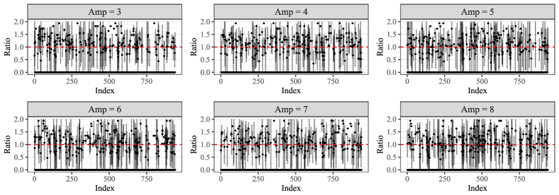
Figure 28: Realized ratios $\mathbb{P}(\Pi_{j}\geq 1/2)/\mathbb{E}[\Pi_{j}]$ with $95\%$ confidence intervals estimated from $200$ repetitions. The experiment setting is the same as in Figure 7.

Large-scale simulation from Section 4

Figure 30 plots the realized ratio between $\mathbb{P}(\Pi_{j}\geq 0.5)$ and $\mathbb{E}[\Pi_{j}]$ (with $95\%$ confidence intervals); Figure 31 and 32 are the (pooled) histograms of all nonzero null $\Pi_{j}$’s and the number of false discoveries.

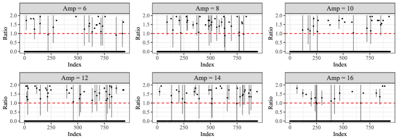
Figure 30: Realized ratios $\mathbb{P}(\Pi_{j}\geq 1/2)/\mathbb{E}[\Pi_{j}]$ with $95\%$ confidence intervals estimated from $200$ repetitions. The experiment setting is the same as in Figure 14.

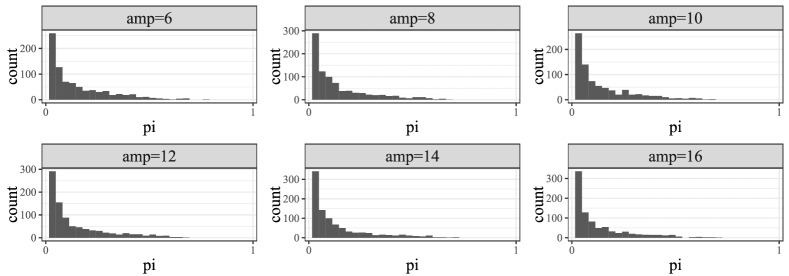
Figure 31: Pooled histograms of all nonzero null $\Pi_{j}$’s for different signal amplitudes. The experiment setting is the same as in Figure 14.

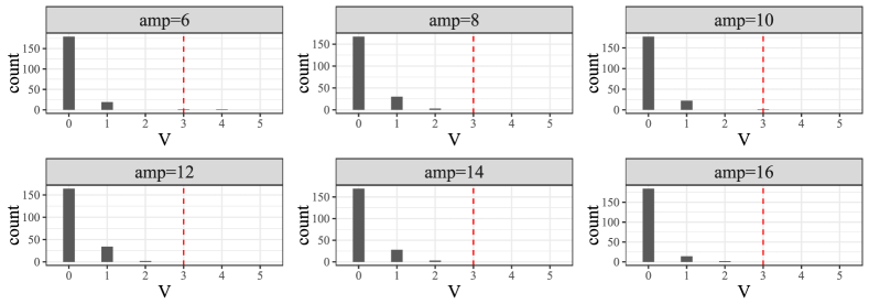
Figure 32: Histograms of the number of false discoveries $V$ for different signal amplitudes. The experiment setting is the same as in Figure 14.

D.3 Additional tables

		V
Amplitude	Method	0	1	2	3	4	5	6	7	8	9	10+
	Derandomized Knockoffs	147	42	9	1	1	0	0	0	0	0	0
3	Vanilla Knockoffs	119	47	17	11	5	1	0	0	0	0	0
	Derandomized Knockoffs	159	33	8	0	0	0	0	0	0	0	0
4	Vanilla Knockoffs	117	42	24	8	6	1	1	0	1	0	0
	Derandomized Knockoffs	163	31	3	3	0	0	0	0	0	0	0
5	Vanilla Knockoffs	116	42	23	11	5	1	1	1	0	0	0
	Derandomized Knockoffs	153	35	10	2	0	0	0	0	0	0	0
6	Vanilla Knockoffs	110	45	30	7	1	3	3	0	1	0	0
	Derandomized Knockoffs	145	48	6	1	0	0	0	0	0	0	0
7	Vanilla Knockoffs	102	44	20	18	8	5	3	0	0	0	0
	Derandomized Knockoffs	152	40	7	1	0	0	0	0	0	0	0
8	Vanilla Knockoffs	102	51	22	10	7	3	3	0	1	1	0

Table 3: Frequencies (out of $200$ runs) of the number of false discoveries. The simulation setting is the same as in Figure 5.

		V
Amplitude	Method	0	1	2	3	4	5	6	7	8	9	10	11	12	13	14	15	16+
	Derandomized Knockoffs	62	57	45	21	15	0	0	0	0	0	0	0	0	0	0	0	0
3	Vanilla Knockoffs	57	43	35	23	27	6	4	4	0	0	1	0	0	0	0	0	0
	Derandomized Knockoffs	41	77	51	22	8	1	0	0	0	0	0	0	0	0	0	0	0
4	Vanilla Knockoffs	49	48	44	20	17	11	7	1	2	1	0	0	0	0	0	0	0
	Derandomized Knockoffs	51	65	53	17	10	2	1	1	0	0	0	0	0	0	0	0	0
5	Vanilla Knockoffs	52	45	40	24	18	8	4	7	0	2	0	0	0	0	0	0	0
	Derandomized Knockoffs	48	69	44	22	15	1	1	0	0	0	0	0	0	0	0	0	0
6	Vanilla Knockoffs	47	44	35	23	17	15	6	6	4	3	0	0	0	0	0	0	0
	Derandomized Knockoffs	57	61	53	20	6	2	1	0	0	0	0	0	0	0	0	0	0
7	Vanilla Knockoffs	49	40	39	26	21	11	10	3	1	0	0	0	0	0	0	0	0
	Derandomized Knockoffs	40	71	54	20	9	5	1	0	0	0	0	0	0	0	0	0	0
8	Vanilla Knockoffs	45	54	44	21	13	11	6	2	1	1	0	1	0	0	0	1	0

Table 4: Frequencies (out of $200$ runs) of the number of false discoveries. The simulation setting is the same as in Figure 7.

		V
Amplitude	Method	0	1	2	3	4	5	6	7	8+
	Derandomized Knockoffs	196	4	0	0	0	0	0	0	0
10	Vanilla Knockoffs	171	20	9	0	0	0	0	0	0
	Derandomized Knockoffs	196	4	0	0	0	0	0	0	0
15	Vanilla Knockoffs	172	18	6	2	1	1	0	0	0
	Derandomized Knockoffs	194	6	0	0	0	0	0	0	0
20	Vanilla Knockoffs	166	18	9	4	3	0	0	0	0
	Derandomized Knockoffs	192	8	0	0	0	0	0	0	0
25	Vanilla Knockoffs	152	22	15	6	4	0	0	1	0
	Derandomized Knockoffs	193	7	0	0	0	0	0	0	0
30	Vanilla Knockoffs	161	25	7	5	1	0	0	1	0
	Derandomized Knockoffs	190	9	1	0	0	0	0	0	0
35	Vanilla Knockoffs	155	27	4	10	3	1	0	0	0

Table 5: Frequencies (out of $200$ runs) of the number of false discoveries. The simulation setting is the same as in Figure 10.

		V
Amplitude	Method	0	1	2	3	4	5	6	7	8	9	10+
	Derandomized Knockoffs	179	19	0	1	1	0	0	0	0	0	0
6	Vanilla Knockoffs	127	35	19	10	5	4	0	0	0	0	0
	Derandomized Knockoffs	167	30	3	0	0	0	0	0	0	0	0
8	Vanilla Knockoffs	111	35	28	15	9	0	1	1	0	0	0
	Derandomized Knockoffs	177	22	0	1	0	0	0	0	0	0	0
10	Vanilla Knockoffs	125	37	15	14	5	2	1	0	0	1	0
	Derandomized Knockoffs	164	34	2	0	0	0	0	0	0	0	0
12	Vanilla Knockoffs	123	42	18	6	6	3	0	0	2	0	0
	Derandomized Knockoffs	169	28	3	0	0	0	0	0	0	0	0
14	Vanilla Knockoffs	125	42	18	7	3	3	1	1	0	0	0
	Derandomized Knockoffs	184	14	2	0	0	0	0	0	0	0	0
16	Vanilla Knockoffs	126	45	17	7	4	0	1	0	0	0	0

Table 6: Frequencies (out of $200$ runs) of the number of false discoveries. The simulation setting is the same as in Figure 14.

References

- Barber et al., (2015) Barber, R. F., Candès, E. J., et al. (2015). Controlling the false discovery rate via knockoffs. The Annals of Statistics, 43(5):2055–2085.
- Barber et al., (2019) Barber, R. F., Candès, E. J., et al. (2019). A knockoff filter for high-dimensional selective inference. The Annals of Statistics, 47(5):2504–2537.
- Belloni et al., (2014) Belloni, A., Chernozhukov, V., and Hansen, C. (2014). Inference on treatment effects after selection among high-dimensional controls. The Review of Economic Studies, 81(2):608–650.
- Benjamini and Yekutieli, (2001) Benjamini, Y. and Yekutieli, D. (2001). The control of the false discovery rate in multiple testing under dependency. Annals of statistics, pages 1165–1188.
- Bhattacharjee et al., (2001) Bhattacharjee, A., Richards, W. G., Staunton, J., Li, C., Monti, S., Vasa, P., Ladd, C., Beheshti, J., Bueno, R., Gillette, M., et al. (2001). Classification of human lung carcinomas by mrna expression profiling reveals distinct adenocarcinoma subclasses. Proceedings of the National Academy of Sciences, 98(24):13790–13795.
- Breiman, (1996) Breiman, L. (1996). Bagging predictors. Machine learning, 24(2):123–140.
- Breiman, (1999) Breiman, L. (1999). Using adaptive bagging to debias regressions. Technical report, Technical Report 547, Statistics Dept. UCB.
- Breiman, (2001) Breiman, L. (2001). Random forests. Machine learning, 45(1):5–32.
- Bühlmann et al., (2002) Bühlmann, P., Yu, B., et al. (2002). Analyzing bagging. The Annals of Statistics, 30(4):927–961.
- Bycroft et al., (2018) Bycroft, C., Freeman, C., Petkova, D., Band, G., Elliott, L. T., Sharp, K., Motyer, A., Vukcevic, D., Delaneau, O., O’Connell, J., et al. (2018). The uk biobank resource with deep phenotyping and genomic data. Nature, 562(7726):203–209.
- Candès et al., (2018) Candès, E., Fan, Y., Janson, L., and Lv, J. (2018). Panning for gold:‘model-x’knockoffs for high dimensional controlled variable selection. Journal of the Royal Statistical Society: Series B (Statistical Methodology), 80(3):551–577.
- Candès and Sur, (2020) Candès, E. J. and Sur, P. (2020). The phase transition for the existence of the maximum likelihood estimate in high-dimensional logistic regression. The Annals of Statistics, 48(1):27–42.
- Crouch et al., (2017) Crouch, L. A., Dodd, L. E., and Proschan, M. A. (2017). Controlling the family-wise error rate in multi-arm, multi-stage trials. Clinical Trials, 14(3):237–245.
- Duan et al., (2020) Duan, B., Ramdas, A., and Wasserman, L. (2020). Familywise error rate control by interactive unmasking. arXiv preprint arXiv:2002.08545.
- Dudoit and Van Der Laan, (2007) Dudoit, S. and Van Der Laan, M. J. (2007). Multiple testing procedures with applications to genomics. Springer Science & Business Media.
- Dunn, (1961) Dunn, O. J. (1961). Multiple comparisons among means. Journal of the American statistical association, 56(293):52–64.
- Efron and Gong, (1983) Efron, B. and Gong, G. (1983). A leisurely look at the bootstrap, the jackknife, and cross-validation. The American Statistician, 37(1):36–48.
- Eklund et al., (2016) Eklund, A., Nichols, T. E., and Knutsson, H. (2016). Cluster failure: Why fmri inferences for spatial extent have inflated false-positive rates. Proceedings of the national academy of sciences, 113(28):7900–7905.
- Elliott et al., (2010) Elliott, K. S., Zeggini, E., McCarthy, M. I., Gudmundsson, J., Sulem, P., Stacey, S. N., Thorlacius, S., Amundadottir, L., Grönberg, H., Xu, J., et al. (2010). Evaluation of association of hnf1b variants with diverse cancers: collaborative analysis of data from 19 genome-wide association studies. PloS one, 5(5):e10858.
- Fan and Lv, (2008) Fan, J. and Lv, J. (2008). Sure independence screening for ultrahigh dimensional feature space. Journal of the Royal Statistical Society: Series B (Statistical Methodology), 70(5):849–911.
- Fithian et al., (2014) Fithian, W., Sun, D., and Taylor, J. (2014). Optimal inference after model selection. arXiv preprint arXiv:1410.2597.
- Gao et al., (2018) Gao, C., Sun, H., Wang, T., Tang, M., Bohnen, N. I., Müller, M. L., Herman, T., Giladi, N., Kalinin, A., Spino, C., et al. (2018). Model-based and model-free machine learning techniques for diagnostic prediction and classification of clinical outcomes in parkinson’s disease. Scientific reports, 8(1):1–21.
- Goeman et al., (2011) Goeman, J. J., Solari, A., et al. (2011). Multiple testing for exploratory research. Statistical Science, 26(4):584–597.
- Guo et al., (2014) Guo, W., He, L., Sarkar, S. K., et al. (2014). Further results on controlling the false discovery proportion. The Annals of Statistics, 42(3):1070–1101.
- Haiman et al., (2011) Haiman, C. A., Chen, G. K., Blot, W. J., Strom, S. S., Berndt, S. I., Kittles, R. A., Rybicki, B. A., Isaacs, W. B., Ingles, S. A., Stanford, J. L., et al. (2011). Characterizing genetic risk at known prostate cancer susceptibility loci in african americans. PLoS Genet, 7(5):e1001387.
- Hochberg, (1988) Hochberg, Y. (1988). A sharper bonferroni procedure for multiple tests of significance. Biometrika, 75(4):800–802.
- Hofner and Hothorn, (2015) Hofner, B. and Hothorn, T. (2015). stabs: Stability selection with error control. R package version R package version 0.5-1.
- Holm, (1979) Holm, S. (1979). A simple sequentially rejective multiple test procedure. Scandinavian journal of statistics, pages 65–70.
- Huber, (2018) Huber, M. (2018). Halving the bounds for the markov, chebyshev, and chernoff inequalities using smoothing. arXiv preprint arXiv:1803.06361.
- Hui et al., (2014) Hui, J., Xu, Y., Yang, K., Liu, M., Wei, D., Zhang, Y., Shi, X. H., Yang, F., Wang, N., Wang, X., et al. (2014). Study of genetic variants of 8q21 and 8q24 associated with prostate cancer in jing-jin residents in northern china. Clinical Laboratory, 60(4):645–652.
- Janson et al., (2016) Janson, L., Su, W., et al. (2016). Familywise error rate control via knockoffs. Electronic Journal of Statistics, 10(1):960–975.
- Kaikkonen et al., (2018) Kaikkonen, E., Rantapero, T., Zhang, Q., Taimen, P., Laitinen, V., Kallajoki, M., Jambulingam, D., Ettala, O., Knaapila, J., Boström, P. J., et al. (2018). Ano7 is associated with aggressive prostate cancer. International journal of cancer, 143(10):2479–2487.
- Karlin and Rinott, (1980) Karlin, S. and Rinott, Y. (1980). Classes of orderings of measures and related correlation inequalities. i. multivariate totally positive distributions. Journal of Multivariate Analysis, 10(4):467–498.
- Kote-Jarai et al., (2011) Kote-Jarai, Z., Al Olama, A. A., Giles, G. G., Severi, G., Schleutker, J., Weischer, M., Campa, D., Riboli, E., Key, T., Gronberg, H., et al. (2011). Seven prostate cancer susceptibility loci identified by a multi-stage genome-wide association study. Nature genetics, 43(8):785–791.
- Lambert et al., (2013) Lambert, J.-C., Ibrahim-Verbaas, C. A., Harold, D., Naj, A. C., Sims, R., Bellenguez, C., Jun, G., DeStefano, A. L., Bis, J. C., Beecham, G. W., et al. (2013). Meta-analysis of 74,046 individuals identifies 11 new susceptibility loci for alzheimer’s disease. Nature genetics, 45(12):1452.
- Lee et al., (2013) Lee, J. D., Sun, D. L., Sun, Y., and Taylor, J. E. (2013). Exact post-selection inference with the lasso. arXiv preprint arXiv:1311.6238, 354:355.
- Ma, (2017) Ma, C. (2017). Semi-penalized inference with direct false discovery rate control for high-dimensional aft model. In 2017 IEEE 2nd International Conference on Big Data Analysis (ICBDA), pages 48–52. IEEE.
- Meijer and Goeman, (2016) Meijer, R. J. and Goeman, J. J. (2016). Multiple testing of gene sets from gene ontology: possibilities and pitfalls. Briefings in bioinformatics, 17(5):808–818.
- Meinshausen and Bühlmann, (2010) Meinshausen, N. and Bühlmann, P. (2010). Stability selection. Journal of the Royal Statistical Society: Series B (Statistical Methodology), 72(4):417–473.
- Monti et al., (2003) Monti, S., Tamayo, P., Mesirov, J., and Golub, T. (2003). Consensus clustering: a resampling-based method for class discovery and visualization of gene expression microarray data. Machine learning, 52(1-2):91–118.
- Polikar, (2012) Polikar, R. (2012). Ensemble learning. In Ensemble machine learning, pages 1–34. Springer.
- Ren and Candès, (2020) Ren, Z. and Candès, E. (2020). Knockoffs with side information. arXiv preprint arXiv:2001.07835.
- Rokach, (2010) Rokach, L. (2010). Ensemble-based classifiers. Artificial intelligence review, 33(1-2):1–39.
- Romano et al., (2010) Romano, J. P., Wolf, M., et al. (2010). Balanced control of generalized error rates. The Annals of Statistics, 38(1):598–633.
- Schumacher et al., (2018) Schumacher, F. R., Al Olama, A. A., Berndt, S. I., Benlloch, S., Ahmed, M., Saunders, E. J., Dadaev, T., Leongamornlert, D., Anokian, E., Cieza-Borrella, C., et al. (2018). Association analyses of more than 140,000 men identify 63 new prostate cancer susceptibility loci. Nature genetics, 50(7):928.
- (46) Sesia, M., Bates, S., Candès, E., Marchini, J., and Sabatti, C. (2020a). Controlling the false discovery rate in gwas with population structure. bioRxiv.
- (47) Sesia, M., Katsevich, E., Bates, S., Candès, E., and Sabatti, C. (2020b). Multi-resolution localization of causal variants across the genome. Nature Communications, 11(1):1–10.
- Sesia et al., (2019) Sesia, M., Sabatti, C., and Candès, E. J. (2019). Gene hunting with hidden markov model knockoffs. Biometrika, 106(1):1–18.
- Shah and Samworth, (2013) Shah, R. D. and Samworth, R. J. (2013). Variable selection with error control: another look at stability selection. Journal of the Royal Statistical Society: Series B (Statistical Methodology), 75(1):55–80.
- Sham and Purcell, (2014) Sham, P. C. and Purcell, S. M. (2014). Statistical power and significance testing in large-scale genetic studies. Nature Reviews Genetics, 15(5):335–346.
- Spector and Janson, (2020) Spector, A. and Janson, L. (2020). Private communication.
- Srinivasan et al., (2019) Srinivasan, A., Zhan, X., and Xue, L. (2019). Compositional knockoff filter for high-dimensional regression analysis of microbiome data. bioRxiv, page 851337.
- Strehl and Ghosh, (2002) Strehl, A. and Ghosh, J. (2002). Cluster ensembles—a knowledge reuse framework for combining multiple partitions. Journal of machine learning research, 3(Dec):583–617.
- Thomas et al., (2009) Thomas, G., Jacobs, K. B., Kraft, P., Yeager, M., Wacholder, S., Cox, D. G., Hankinson, S. E., Hutchinson, A., Wang, Z., Yu, K., et al. (2009). A multistage genome-wide association study in breast cancer identifies two new risk alleles at 1p11. 2 and 14q24. 1 (rad51l1). Nature genetics, 41(5):579.
- Tian et al., (2018) Tian, X., Loftus, J. R., and Taylor, J. E. (2018). Selective inference with unknown variance via the square-root lasso. Biometrika, 105(4):755–768.
- Tibshirani et al., (2016) Tibshirani, R. J., Taylor, J., Lockhart, R., and Tibshirani, R. (2016). Exact post-selection inference for sequential regression procedures. Journal of the American Statistical Association, 111(514):600–620.
- Tukey, (1980) Tukey, J. W. (1980). We need both exploratory and confirmatory. The American Statistician, 34(1):23–25.
- Voorman et al., (2014) Voorman, A., Shojaie, A., and Witten, D. (2014). Inference in high dimensions with the penalized score test. arXiv preprint arXiv:1401.2678.
- Wang et al., (2015) Wang, M., Takahashi, A., Liu, F., Ye, D., Ding, Q., Qin, C., Yin, C., Zhang, Z., Matsuda, K., Kubo, M., et al. (2015). Large-scale association analysis in asians identifies new susceptibility loci for prostate cancer. Nature communications, 6(1):1–7.
- Wasserman and Roeder, (2009) Wasserman, L. and Roeder, K. (2009). High dimensional variable selection. Annals of statistics, 37(5A):2178.
- Wu et al., (2010) Wu, J., Devlin, B., Ringquist, S., Trucco, M., and Roeder, K. (2010). Screen and clean: a tool for identifying interactions in genome-wide association studies. Genetic Epidemiology: The Official Publication of the International Genetic Epidemiology Society, 34(3):275–285.
- Zhao et al., (2014) Zhao, C.-X., Liu, M., Xu, Y., Yang, K., Wei, D., Shi, X.-H., Yang, F., Zhang, Y.-G., Wang, X., Liang, S.-Y., et al. (2014). 8q24 rs4242382 polymorphism is a risk factor for prostate cancer among multi-ethnic populations: evidence from clinical detection in china and a meta-analysis. Asian Pacific Journal of Cancer Prevention, 15(19):8311–8317.