Hiperfact: In-Memory High Performance Fact Processing - Rethinking the Rete Inference Algorithm

Abstract

The Rete forward inference algorithm forms the basis for many rule engines deployed today, but it exhibits the following problems: (1) the caching of all intermediate join results, (2) the processing of all rules regardless of the necessity to do so (stemming from the underlying forward inference approach), (3) not defining the join order of rules and its conditions, significantly affecting the final run-time performance, and finally (4) pointer chasing due to the overall network structure, leading to inefficient usage of the CPU caches caused by random access patterns. The Hiperfact approach aims to overcome these shortcomings by (1) choosing cache efficient data structures on the primary rank 1 fact index storage and intermediate join result storage levels, (2) introducing island fact processing for determining the join order by ensuring minimal intermediate join result construction, and (3) introducing derivation trees to allow for parallel read/write access and lazy rule evaluation. The experimental evaluations show that the Hiperfact prototype engine implementing the approach achieves significant improvements in respect to both inference and query performance. Moreover, the proposed Hiperfact engine is compared to existing engines in the context of a comprehensive benchmark.

1 Introduction

The Rete inference algorithm [11] forms the basis for most rule engines deployed today [17, 31, 15, 29]. Existing research deal with the extension of the core algorithm for specific applications [33, 30, 2], while other approaches cover the deficiencies of the Rete inference approach, [19, 28, 6, 9]. The main problems of the Rete inference algorithm can be summarized as follows: (1) All intermediate results are cached, regardless of the necessity to do so, leading to ballooning of consumed RAM. (2) All rules passed to the Rete rule engine will be evaluated, potentially leading to inferred facts that are irrelevant and might never be used as input, which is the drawback of the applied forward chaining inference approach. (3) Rete does not deal with join ordering, which affects the final run-time performance. (4) The network structure of the Rete algorithm does not facilitate efficient CPU cache usage, as pointer chasing causes poor usage of prefetched data from the CPU caches (L1/L2). Regarding (3), join ordering falls under the topic of query optimization. As efficient fact retrieval is central to identifying rules having their conditions satisfied, it is critical for inference. Recent work [14, 12] focus on efficient query execution, but treats the topic independently from inference.

The original Rete algorithm [11] proposes the triple fact structure as the basis for modeling facts, which is the de facto data structure for reasoning within the Semantic Web’s Resource Description Framework (RDF) domain [10, 14]. While column-oriented storage approaches are discussed in context of RDF / triple stores [18], it is usually only within the context of the fact index layer. The dependent layers on top: intermediate join result and the final result data structure are not considered. We argue that by explicitly decoupling the data store (triple store) and the inference fact processing step, potential performance gains are missed due to not considering the optimization techniques that are possible within the layers in-between these two processes. Here both the underlying data storage techniques and the inference processing technique need to coordinate for achieving better inference performance. For example in [10], not all storage proposals support inference, showing the disconnect of storage design and inference. It is imperative to consider fact storage techniques in regards to inference as well. Furthermore, Rete does not consider compression when processing facts as it assumes that the triples are fully materialized during processing. As shown in [1], applying operations directly on compressed blocks without decompressing has significant impact on the final performance. Again, all three layers of the storage, i.e. fact index, intermediate joins, and final result sets, need to coordinate when dealing with compressed data types.

Thread and data parallelization can both be applied for further improving the performance of the inference process. Existing works [23, 2] deal with parallelizing the core Rete algorithm. In addition to parallelizing the core fact processing step with multiple worker threads during the fact processing step, we study where and how data parellelism – namely vectorization – can be applied.

In order to meet the mentioned challenges above we propose Hiperfact, a comprehensive architecture (data structures and algorithms) for high performance fact processing covering forward inference and query execution, allowing monotonic interactive data exploration by supporting incremental inference. We adapt Stylus’ [14] strong typing idea both on the fact type level and the data value type level. This strong typed design allows for improved query execution and parallel fact insertions. We adopt Inferray’s [32] cache efficiency idea in all levels of the fact storage and employ both thread parallelism and additionally data parallelism (vectorization), and column-oriented storage to improve throughput. We do not limit the rule model to a specific domain and stay as generic as possible. Concretely, the contributions in this paper tackling the aforementioned problems Rete exhibits are as follows:

• Fork Join Model Instances and Block Sizing We illustrate many instances of the fork join model for thread parallelism and show opportunities for applying data parallelism in the context of fact processing. These applications are at the level of both, the single fact and inter-fact processing layers. Core to the fork join model is determining the data block size each work thread should take as input.

• Island Fact Processing. We propose an overall island fact processing method that, together with sort keys, finds the optimal order for rule processing and underlying condition lookup and joins. To do so we determine the best join order for inter-fact processing using cardinality estimates derived from the underlying rank 1 indices and other condition-associated metrics.

• Derivation Trees. We define derivation trees in order to detect which rules can be skipped for processing (laziness property) and identify parallel write opportunities to the underlying rank 1 indices.

• Evaluation. We evaluate the proposed techniques and concepts internally and against other existing rule engine implementations using OpenRuleBench [21].

1.1 Motivation

In this section we motivate Hiperfact by summarizing the Rete inference algorithm and the aforementioned problems.

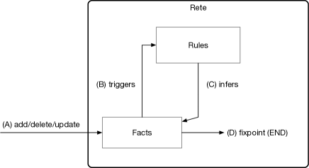
Figure 1: Rete Inference Loop

The Rete algorithm includes an inference step depicted in Figure 1. The goal of it being to infer derived facts each time facts are modified (Figure 1 A). After each modification, user-defined rules can be triggered (Figure 1 B). If so, facts can be inferred (Figure 1 C), after which the loop continues until a fixpoint is reached where no more facts can be inferred (Figure 1 D). At this point the inference step concludes, waiting until the next fact modification event occurs. Note that the triggering of rules (B) can be omitted if no rule conditions are matched, in that case the fixpoint (D) is directly reached.

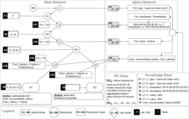
Figure 2: Rete Basic Components

The data structure of Rete is depicted in Figure 2 and is divided into two components: the alpha and the beta network. The alpha network is designed to handle two issues. First, it is responsible for indexing the facts entered into Rete, and secondly it breaks down the user-defined rules into their elementary conditions on which to filter facts with. This indexing process is conducted based on the triple fact structure: (id, attribute, value) respected by both the facts being entered as well as by the conditions making up the rules. This triple structure is divided into three id, attribute, and value parts. The id marks the unique identifier to track a certain entity. Each entity has at least one but unbounded attribute, value pairs. Rule conditions can contain optional variable parts, prepended with the ’?’ character. For example, in Figure 2 the A3 alpha node handles all facts that match the pattern (?id, value, ?value), meaning all entities with the attribute literal value and any kind of associated value on the id and value parts are passed to the alpha node and processed through the network from there. This is one of the two pattern matching tasks performed by Rete, in this case the pattern matching is conducted between fact and conditions, handled by the alpha nodes.

The beta network handles the second pattern matching task of Rete starting with facts being passed from the alpha nodes to the join nodes. These join nodes deal with the joining of facts that match based on common logical variables. For example, the join node J2 joins all facts coming from A2 and B1 and joins based on the common variables ?id. These variables can occur in any of the three fact places. As facts are joined together, they are passed down to the attached beta nodes and stored there as tokens (i.e. T2 in Figure 2). Any join nodes attached to these beta nodes are then triggered, using the newly added tokens as input for the join process. Triggering those join nodes means that facts are retrieved from the associated alpha nodes. These facts are then joined with the aforementioned tokens to perform the join operation. Continuing the previous example, the beta node B2 passes down the tokens to J3, which fetches the facts from A3 (f5 and f6) and performs an equi-join based on the common variables ?id. The results of these join operations are passed to B3. This join process is repeated until either no more successful joins can be performed or a production node is activated (see R1 and R2 in Figure 2). Triggering a production node means the associated rule is executed (corresponding to Figure 1 B), after which new facts could be inferred from (corresponding to Figure 1 C). Entering these facts causes the fact processing through the alpha network to be triggered, thus another fact join processing loop to be started. The fixpoint is then reached (Figure 1 D) when the join process in the beta network stops due to no successful joins being possible. The inference loop of Figure 1 is designed to be implemented by both the alpha network and beta network working together.

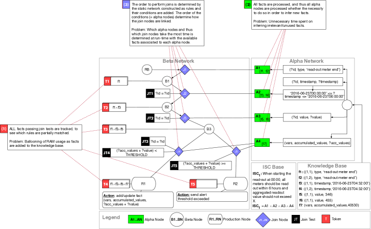
Figure 3: Rete Problems

Based on this foundation we will summarize the common problems Rete has (as annotated in Figure 3). (P1) The first problem concerns the tracking of partial rule matches, represented as tokens under the respective beta nodes. The cost of maintaining these tokens, especially in a pure in-memory setting, is the ballooning in RAM usage. The design trade-off being made here is that through sacrificing storage space, the process of re-joining facts is avoided and thus no wasted joins are performed. (P2) The second problem is related to the alpha network, specifically the processing of all facts, regardless of the necessity to do so in regards to the queries that are in effect. In fact, there is no notion of queries in Rete. Rete’s rule system could be used for defining queries, where the action part is empty, but this is not explicitly defined. Since there is no way to connect governing queries with the facts that are required to answer them, there is no filtering process to know which set of inference rules are inactive and thus know which facts to ignore. When there is an ability to skip processing such facts, wasted time spent on those unneccessary facts can be avoided. (P3) The order to perform joins is statically pre-determined at the time the network is built at initialization. This step happens when the rules are added to the Rete system before the inference loop is triggered. Thus, the order of the rules being added affects the order of alpha nodes being created. The alpha nodes in turn help build up the beta network, starting with the definition of join nodes, beta nodes and finally the production nodes. One critical aspect being ignored in this regard is the information available at run-time: the actual number of facts (cardinality) associated to the alpha nodes that actually serve as input in all of the join operations. Re-ordering the way the facts are joined together based on this cardinality alone affects the run-time performance of the inference loop. (P4) The final problem is the incompatibility of Rete’s network structure towards how modern CPUs and RAM work. Figure 4 shows a full inference step showing the nodes being processed starting from the alpha node A1. As each node is being looked up, in modern memory systems [7] data elements are not simply looked up atomically, but due to pre-fetching, neighbor entries in the same array will be fetched as well. The assumption here is that through spatial locality that those pre-fetched neighbor nodes will be required for later CPU processing as well. This assumption does not work with Rete, as only that single node is accessed and processed before another unrelated lookup (in terms of memory location) is performed for the associated nodes to continue fact processing (join node J1 in this example). The main problem here is that the pre-fetching behaviour of modern CPUs is not being exploited in Rete, thus a new structural design is required to exploit that behaviour. Another related problem is that basic Rete does not prescribe the storage level design in terms of how the facts are stored. It only prescribes that the alpha nodes are used to start the processing of facts, but does not determine how the facts are fetched in which order, nor how the facts are stored in the knowledge base. These issues are important topics as well, that we will discuss in this paper. Note that the Rete algorithm is designed to be an in-memory inference algorithm. Realizing the fact storage in another context, such as in a persisted or distributed fashion is not part of this work.

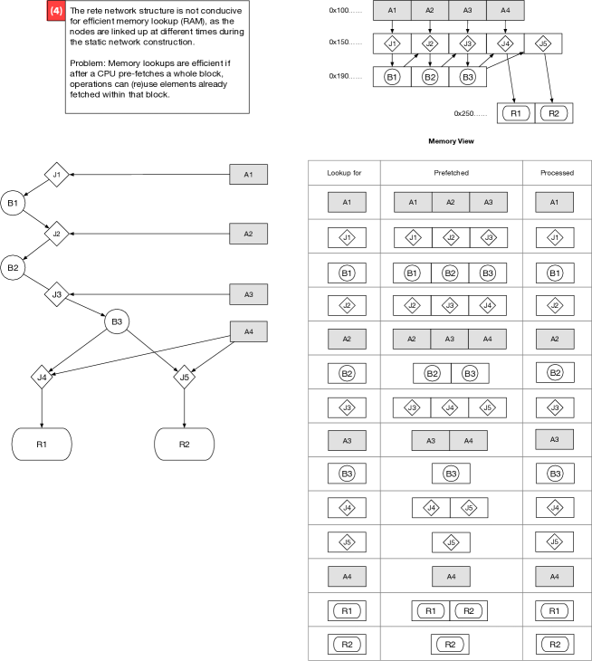
Figure 4: Rete Memory Access Patterns

This paper addresses each of the aforementioned problems by redesigning the core componenets making up the Rete algorithm. The resulting data structures and algorithms deviate from Rete that we give it a new name under which the collection of changes constitute a novel inference and querying algorithm: Hiperfact. In the next section we will describe the baseline Hiperfact Architecture, which addresses all of the problems mentioned in this section.

2 Hiperfact Architecture

In this section we highlight the individual components required for realizing the overall Hiperfact architecture as shown in Figure 5 and discuss relevant technical details. We follow the design guidelines – choke points [8] – that are critical for achieving good performance for query execution and thus inference which motivated the chosen components. Specifically, we focus on (1) estimating cardinality, (2) choosing the right join order, (3) parallelism and (4) result reuse. The components discussed in this section will cover some or several of these guidelines.

Figure 5: Hiperfact Architecture Overview

As shown in Figure 5, the focus of Hiperfact is less on executing specific languages, such as Datalog or SPARQL, but more on the underlying low-level process of efficient pattern matching, joining, processing and aggregating facts before inferring new facts based on matched results. As long as a translation path to the model of facts, conditions and rules as defined in this section exists, then the Hiperfact engine can be used for execution of such queries and rules.

2.1 Preliminaries

We start with preliminary definitions that underly all the components, starting with the definition of facts.

Definition 1

[Fact] Based on Rete’s [11] and RDF’s triple fact structure, we extend a fact to be a quintuple structured data item to represent a concrete aspect of an event. Facts are used as input for Hiperfact to derive more facts, as well as to answer queries and has the following structure:

(<fact type> <id> <attr> <val> <value type>)

The <fact type> allows facts to be strongly typed, which is beneficial for two reasons. First, to store facts in distinct namespaces for avoiding unnecessary pattern matches on common <id>, <attr> or <val> fact components that are not conceptually related. Secondly, it serves as the basis for the derivation tree allowing parallel lazy rule evaluation (see Section 2.4). <value type> is one of {string, int32, int64, uint32, uint64, float, double, bool}.

Example: Fact (City “city1” “name” “New York” string) represents the data item with type City holding the name of the city “New York” under the id “city1”. Fact (Person “person1” “name” “Jane” string) represents a person named “Jane” stored under the namespace Person.

Definition 2

[Condition] A condition specifies a pattern to perform fact lookups, returning all facts matching that pattern and follows the same structure as a fact with the possibility of having named logical variables populating the <id>, <attr> and <val> fact components. Several conditions can be joined together having the same named logical variables. A named logical variable starts with the “?” symbol. An optional component <tests> is added to the condition to house a set of join tests (see Definition 9).

Example: The conditions (Person ?p1 “livesIn” ?city string) and (City ?city “name” ?name string) perform fact lookups on both Person and City where the logical variable ?city match (i.e. are equal). Furthermore, the logical variables ?p1 and ?name are mapped to actual person ids and city names where those conditions are satisfied.

Definition 3

[Rule] A rule holds a collection of conditions for specifying the facts the rule is to be applied to, and an action part to process the matched facts:

$$(\texttt{conditions = <c1, ..., cN>},\texttt{action = <a1, ..., aN>})$$

Actions can be either external for connecting the matched facts to external systems (e.g. monitoring/alerting systems) or internal for adding new or modifying existing facts. The focus of this paper is on internal actions as it pertains to fact processing: add(new <fact>), delete(old <fact>), and replace(old <fact>, new <fact>).

Example: Given conds = [(DailySales ?s “profitEUR” ?p double), (DailySales ?s “EURUSD” ?f double)] and actions = [add(DailySales ?s “profitUSD” ($?p\,*\,?f$) double)], Rule(conds, actions) defines a rule that derives the absolute profit in USD from existing facts.

2.2 Fact-Level Rank 1 Index

One responsibility of a fact storage layer is the ability to query that storage layer. In this context, we have a knowledge base that can be queried to retrieve facts. This is not a topic discussed explicitly by Rete, the only assumption being that alpha nodes know how to retrieve facts that match the pattern associated to the alpha node. Especially in an in-memory setting, that efficient usage of both CPU and modern RAM is critical to keep performance high, which basic Rete completely ignores. Subsequent fact processing work depend on this layer to function efficiently. We call this layer: the rank 1 index. The main driver of this component is (P4) where we try to efficiently use pre-fetched data in order to improve overall fact lookup operations. The rank 1 index is the primary data structure for storing and retrieving facts. The relevant design choke point estimating cardinality serves as the main guiding principle in designing this component. In Figure 5 we can see that this component serves as input for the component responsible for query optimization: island processing. For this purpose the rank 1 index provides an API focused on fact retrieval by conditions. As the condition is the main driver for retrieval of facts, we estimate the cardinality of facts returned by a given condition thus fulfilling this component’s guiding design principle. First, we need to understand a condition’s rank that affects the cardinality of facts to be retrieved.

Definition 4

[Condition Rank (CR)] We define the condition rank (CR) to be equal to the number of concrete values filling the (<id> <attr> <val>) triple part of a condition. The valid CR range is $[0,3]$, where 0 represents a condition that matches all facts. The higher the CR, the more specific the filtered facts are. The maximum is 3 representing all triple components being filled with concrete values. For example, given the condition (City ?id name ?x string), its rank CR((City ?id name ?x string)) = 1 due to only one concrete value found in the attribute part.

The rank 1 index then is a set of inverted indices, one for each triple part of facts: id, attribute, value, allowing for efficient retrieval of facts queried by conditions that have a condition rank of 1 (i.e., have only one slot filled with concrete values). The corresponding lookup function used in later components for retrieving such facts is called the Rank 1 Condition Lookup (R1L), defined as follows:

Definition 5

[Rank 1 Condition Lookup (R1L)] Given a condition c with rank $\texttt{CR}(c)=1$, we define three lookup functions R1L_id(c), R1L_attr(c), R1L_val(c)) to be trivial fetch functions from the inverted index on the corresponding triple component. The R1L can then be defined as:

$$\texttt{R1L}(c)=\begin{cases}\texttt{R1L${}_{id}$}(c),&\text{if }\texttt{CR}(c)=1\,\wedge\,!\texttt{isVar}(c.id)\\ \texttt{R1L${}_{attr}$}(c),&\text{if }\texttt{CR}(c)=1\,\wedge\,!\texttt{isVar}(c.attr)\\ \texttt{R1L${}_{val}$}(c),&\text{if }\texttt{CR}(c)=1\,\wedge\,!\texttt{isVar}(c.val)\\ \{\},&\texttt{otherwise}\end{cases}$$

For example, given c = (Person ?person name ?name string) and CR(c) = 1, the lookup R1L(c) fetches from the attribute inverted index using the keys (Person, string, name) and returns the materialized tight array of all facts that have name as the concrete value in the attribute triple part.

We further define condition cardinality (CCar), to estimate the number of facts a given condition returns.

Definition 6

[Condition Cardinality (CCar)] The condition cardinality is the minimum number of facts indexed on the non-variable triple component parts of the condition. Since the condition cardinality is critical for determining fact processing order, conditions with CR(c) = 0 need to be de-prioritized. Thus, given the set of all triple components $cs=\{id,attr,val\}$, the cardinality of a condition is defined:

$$\texttt{CCar}(c)=\begin{cases}\texttt{inf},&\text{if }\texttt{CR}(c)=0\\ min(\{count(\texttt{R1L${}_{x}$}(c))\mid\forall x\in cs\}),&\text{otherwise }\end{cases}$$

What follows are definitions for Condition Lookup functions of condition rank greater than 1 as well as the generic condition lookup function RL allowing for fact lookup independent of condition rank.

Definition 7

[Rank N $>$ 1 Condition Lookup (RNL)] Given a condition with condition rank $\texttt{CR}(c)>1$, we define its lookup RNL(c) to be an initial R1L(c) lookup on the triple component with the lowest cardinality ($count(\texttt{R1L}(c))=\texttt{CCar}(c)$) and performing a subsequent EQUAL filter on the other triple components of the returned facts that are not variables. The first minimum R1L(c) lookup ensures we start with a small result set, as the subsequent filter results are combined in an AND relation.

Definition 8

[Generic Rank Condition Lookup (RL)] The generic rank condition lookup function (RL) calls the correct rank lookup function depending on the condition’s rank (CR), and is defined as

$$\texttt{RL}(c)=\begin{cases}\texttt{R1L}(c),&\text{if }\texttt{CR}(c)=1\\ \texttt{RNL}(c),&otherwise\end{cases}$$

In this section we highlighted the critical functions required for efficient fact retrieval through estimating cardinality, which will be extensively used in the query optimization phase under the island processing component. For the Hiperfact engine prototype we have three different rank 1 index implementations that expose the common API functions as defined in this section, focusing on cache-efficient loops when retrieving facts. While we do try to keep the storage size small for each fact stored, we do not further optimize on the efficient storage aspect in this work, such as using compression techniques. In a later section we evaluate these differing index implementations in regards to their runtime performance measures: loading, inference, and query time.

The first implementation is a two-level hash table where the first distinguishes on the <fact type> and the second on the concrete fact component. Associated to those keys is a tightly packed array of all matching facts. This can be seen as an inverted index. Since we have three parts to a single fact, i.e., (<id> <attr> <val>), we define an index for each. Notable is the <id> index, which can be seen as the primary fact base where the keys are the <fact type> as well as the unique <id> of the fact. Additionally, to save more space, the actual fact component for which it is being indexed can be removed. For example, on the <val> index we eschew the storage of the <val> part of the quintuple when adding the fact to the tight array inside the inverted index. The same technique is applied to the other two indices. At the time of lookup, the full fact quintuple can be reconstructed adding the missing part using the index key.

The second implementation is a sparse array for holding the two level index. The main insight stems from the <fact type> exhibiting low randomness and thus a simple tight array being sufficient for holding the first level index. The second level index is a sparse array for all possible values being indexed.

The third implementation follows the same tight array design for the <fact type> level and further applies a memory efficient pool of pages that are pre-allocated and provided dynamically for the second level index. The goal is to spend less time on dynamic memory operations due to memory fragmentation, and memcpy operations for accomodating growth at the second level index.

These three implementations focus on dynamic memory management and efficient CPU cache usage for fact retrieval. Possible alternative indexing structures focusing on efficient storage could be bit vectors for further space savings with the cost of having to perform fact id lookups more frequently when performing concrete data filtering.

String Dictionary. Strings are a special consideration as they occur frequently in all facts, i.e., on the <id> and <attr> level, and in the <val> part in case it is of type string. The first line of lookups are equality checks, namely when looking up facts from the inverted index. In order to satisfy that operation and to avoid dynamic memory allocation performing it, we maintain both a string to uint64 string-id radix tree as well as a tightly packed uint64 string-id to string array to index string values. String values are always encoded into an internal dictionary string-id handle before being added to the inverted index. This facilitates cache efficient looping through the index at lookup time as each individual fact becomes fixed size.

2.3 Island Fact Processing

Recall that the basic Rete design is a static processing network that does not take into account the cardinality of inserted facts nor the fact’s type. For this reason, we devised the island processing (see Figure 5) component which focuses on the problems: P1, P3 and P4. On the one hand it eschews the storage vs speed tradeoff of storing pre-joined tokens, with the reason of having low-cost joins for taking into consideration P4’s efficient RAM+CPU usage of pre-fetched data on the underlying rank 1 index, as well as the same considerations made in the design of the island processing component. For most use cases, performing a re-join of existing facts does not hamper performance. In terms of P3, we build a dynamic processing network based on the underlying rank 1 index to process facts in such an order that join effort is kept low. Several join result data structures are discussed to store intermediate join results. The driving idea of the island processing component is that we can process facts in sets grouped by their id part (islands of facts that are directly related) and then joining these islands together. The main problem becomes in which order to process these islands. This component focuses on query optimization issues, i.e., determining the most efficient join order and cost estimation. The latter issue is delegated to the rank 1 index and accumulated into an aggregate cost estimate per island from which the final join order is derived. Core to an efficient fact processing scheme is the cost estimation of joins performed for gathering all relevant facts matching rule conditions. In this section we focus on logical AND relations between rule conditions, and consider OR relations to be independent paths processed concurrently.

Condition lookup complexity estimation The basis for the cost estimation is formed from the lowest rank 1 index level, where the cardinality of individual conditions are known. For example, given c1 = (Book ?x title ‘Title X’ string) and the individual rank 1 cardinalities on the constants $count(\texttt{R1L}_{attr}(c))=10$ for the attribute ‘title’ and $count(\texttt{R1L}_{val}(c))=1$ for the value ‘Title X’, we would be well-advised to start the rank 1 lookup based on $\texttt{R1L}_{val}(c)$ due to its higher selectivity. As per Definition 6, this is indeed the operation being chosen, as $CCar(c)$ equals $1$ by the underlying $\texttt{R1L}_{val}$ lookup. From there the other triple component constants, or constant join tests if they are set, are used for filtering out facts that match. Notice that CCar does not estimate the actual final lookup size, but it does help in picking the triple component with the lowest number of facts stored in the rank 1 index. It is clear that having a higher rank leads to a lower number of results due to higher amount of filtering conducted. Thus we can say that we should prefer higher rank conditions in the beginning of the fact processing to keep the overall join effort low. Keeping the join result as small as possible at all times ensures no unnecessary joins are performed at a later stage.

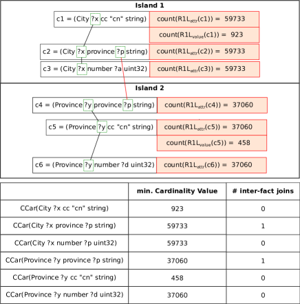
Figure 6: Island-based Inference (fact processing)

Island-based evaluation After having the cardinality estimate of a single condition, we can now extend the estimation to a group of conditions. The conditions inside rules (see Definition 3) usually come in distinct island groups. For example, the conditions (Book ?x title ‘Title X’ string), (Book ?x description ?d string), and (Book ?x author ‘J. D.’ string) can be evaluated together, and represent an island, i.e., Book. ?x is bound to all instances of such books. We consider islands to be all conditions bound to the same variable on the <id> triple component, loosely linked to other islands through common variables at the <value> triple component of one island condition and to any other triple position in one or more other islands. Additionally, for parallel processing purposes, islands can be evaluated separately. Just as we estimate the cost of a single condition, we can now estimate the cost of an island by summing up the individual island conditions. Knowing the island costs before joining them allows picking the best island to start fact lookups with. Thus, for the cost estimation of this particular example, the aggregation would be defined as

$$\begin{split}island_{1}&=\texttt{CCar((Book ?x title `Title X' string))}\\ &+\texttt{CCar((Book ?x description ?d string))}\\ &+\texttt{CCar((Book ?x author `J. D.' string))}\end{split}$$ (1)

Example. Figure 6 shows two islands bound to the <id> variables ?x and ?y. The rank 1 and subsequent rank 2 cardinality cost estimations are shown as well. The aggregate island costs for ?x is higher than ?y’s. For that reason, ?y is evaluated first. The condition lookup sequence for ?y becomes: (Province ?y cc ‘cn’ string) [cost: 458], (Province ?y province ?p string) [cost: 37060], (Province ?y number ?d uint32) [cost: 37060]. We additionally track the number of inter-fact joins between conditions. This number helps us to identify the hook point on which to perform joins between islands. Having evaluated island ?y we can start with island ?x. Then, we continue with the condition that links to island ?x. This would be the condition with the only number of inter-fact joins $>0$, in this case: (Province ?x province ?p string), which includes the unbound variable ?p from the previous island evaluation. Thus the full condition lookup sequence for island ?x becomes: (City ?x province ?p string) [cost: 59733], (City ?x cc ‘cn’ string) [cost: 923], (City ?x number ?a uint32) [cost: 59733]. Note that the first condition’s rank increases at lookup time as the variable ?p is bound and the values are now known. Instead of performing a lookup with cost 59733, we can perform the RNL lookup of rank 2: RNL((City ?x province bound_p string)) $\texttt{count}(?p)$ times, and then combining the results.

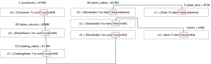
Figure 7: TPC Island-Processing Example

Example: TPC. Figure 7 shows a real-world benchmark example (TPC) for OLAP-based systems. In this particular use case, a shopping data set with customers, sales, store_sales are modeled. Applying the island processing approach to this data set for a query dealing with customer returns would identify the following islands: C with cardinality=100K, SR with cardinality=288K, CS with cardinality=1.4M, SS with cardinality=2.8M, D with cardinality=73K, I with cardinality=18K. The first three islands (C, SR, CS) would be processed first in order of increasing cardinality, and then the final main island (SS). Even though the last two (D,I) have the lowest cardinality, they are only required for the SS island, and are thus delegated until that island is processed.

We can now define the island-based evaluation algorithm (see Algorithm 1), which is split into six phases. Phase 1 is concerned with collecting all conditions that occur in the rule and mapping them according to the <id> variable, associating to it the following metrics: condition rank, number of inter-fact joins and rank 1 cardinality values per <id>, <attr>, <val> triple component (see Definition 6). Conditions are strongly typed, meaning at rule definition time the rule writer has to explicitly set the <fact type>. This reduces ambiguous condition lookups where the same attribute occurs in many namespaces. In Phase 2, all the mapped <id> variables are iterated and for each associated set of conditions an island is initialized, associating to it the total estimated cost (see Equation 1), as well as outgoing and incoming variables. The variables are required in order to know how to join other islands to this one. Additionally, we need to track which condition is mapped to this island. Phase 3 is the main join phase. It starts by sorting the islands by their total cost, and then starting lookups for the first island. When processing an island, conditions are sorted by their cardinality. The rank lookup function (RL) refers to the one defined in Definition 8, performing rank 1-3 lookups depending on the condition’s rank. The join function refers to the join method as defined in Section 2, and includes the logic to choose the appropriate join type. The core part is to join all the separate conditions belonging to the same island on the id position so that the final island can be materialized at a later point. If there is a next island to be joined, its incoming variables are inspected, matched with the corresponding variable name that can be joined. The actual condition and the triple position where to join with is marked and prepared as well (via sorting, such that the corresponding condition is in front). Phase 3 ends once all islands are processed. Phase 4 then materializes and builds the final data structure, allowing user defined actions to be triggered and processed (see ”Action Execution” component in Figure 5). In the original Rete algorithm, all pattern matches for each rule are performed first and rules activated in that process collected in a so called conflict set before the associated actions (e.g., inferring new facts) are triggered. The order in which these rule actions are executed is based on the rule writer’s priority designation, usually a positive integer number where the lower number represents higher priority. In Hiperfact, we follow the derivation trees’ (see Section 2.4) order of evaluation where the dependency of inferred facts to associated rules are explicitly modeled, allowing for concurrent write access to the rank 1 indices. Thus all inferred facts and any actions associated to the current rule are executed once phase 5 is reached. In Phase 5 cleanup operations are performed, mainly releasing stale memory, especially deallocating the final result structure, which has been processed at this point.

Input:

1          $rule$ - Single Rule to be evaluated

2 Begin

3

4// Phase 1: Hash and aggregate statistics on conditions to determine islands and best join order.

5 id_hash $\leftarrow$ {}; attr_hash $\leftarrow$ {}; value_hash $\leftarrow$ {}; island_tracker $\leftarrow$ {};

6 foreach  $condition$ in $rule.conditions$  do

7       cond $\leftarrow$ initialize condition: hash, rank, connected level, rank 1 cardinality values per triple component;

8       $\{id\_hash,attr\_hash,value\_hash\}\leftarrow$ hash cond varname to its triple position;

9

10// Phase 2: Detect all islands and sort by total estimated cost.

11 $islands\leftarrow\{\};$

12 foreach  $varname$ in $id\_hash.keys()$  do

13       conds $\leftarrow id\_hash[varname]$

14       island $\leftarrow$ initialize island from conds: total estimated cost, register outgoing vars, ingoing vars;

15       $islands.add(island)$

16      foreach  $cond$ in $conds$  do

17             it $\leftarrow$ island_tracker[cond.hash] $\mid$ initialize island tracker from cond: count = 0;

18             island_tracker[cond.hash] $\leftarrow$ it.count + 1;

19      

20

21// Phase 3: Process each island, connected through common variables.

22 sort(islands by total_cost);

23 sort(islands[0].conditions by cardinality, connected level);

24 join_result $\leftarrow$ prepare_join(RL(islands[0].conditions[0]));

25 foreach  $island$ in $islands[1:]$  do

26       foreach  $cond$ in $island.conditions[1:]$  do

27             rhs $\leftarrow$ RL(cond);

28             join_result $\leftarrow$ join(join_result, rhs, POS_ID);

29             hash_combine(join_result, cond);

30            

31      if  has_next_island(island)  then

32             connected_vars $\leftarrow$ determine whether cond vars exist for joining to next island using out_vars;

33             if  length(connected_vars) $>$ 0  then

34                   sort(connected_vars by cardinality, connected level);

35                   join_pos $\leftarrow$ connected_vars[0].join_pos;

36            else

37                   join_pos $\leftarrow$ POS_ID;

38            

39            sort(next_island.conditions by cardinality, connected level);

40            

41            rhs $\leftarrow$ RL(next_island.conditions[0]);

42             join_result $\leftarrow$ join(join_result, rhs, join_pos);

43             hash_combine(join_result, cond);

44             island $\leftarrow$ next_island;

45      

46

47// Phase 4: Trigger associated rule actions

48 result $\leftarrow$ build_join_results(join_result);

49 rule.action(result);

50// Phase 5: Cleanup.

51 clean(result);

Algorithm 1 Island-based Evaluation Algorithm

2.3.1 Sort Keys

The previous fact processing approach assumes the following: (a) that the metrics used for ordering the fact evaluation are fixed, and (b) that the sort order for that particular set of metrics is pre-determined. Namely, these are the condition rank, connected level of variables, condition triple component cardinality values, and estimated island cost. With sort keys we extract the ordering logic from the island fact processing algorithm, allowing us to change the set of metrics and the sort order independent of the fact processing algorithm. This decoupling allows us to observe the effect of metric sorting on the overall performance of the inference algorithm, and reduce the number of sort calls made in general (see Section 2.4: derivation trees). For sorting the sort keys we can apply the parallel sort merge algorithm introduced in Section 1, as a sort key is defined as a 32-bit unsigned integer value that is populated with the different metrics in specific bit ranges of that value.

Capping sort key buckets. Before defining the bit ranges, we first discuss the need to bucketize and lower the entropy of the sort key. Instead of using the actual values for filling the individual sort key buckets, which potentially might increase the available bucket size we can opt to keep the relative order between the actual values but mapping them to buckets. For example, having the distinct estimated island scores $\{2043,6833,6833,9700,50900,160000,700000\}$ we observe that fitting the maximum value of 70000 requires 20 bits. Bucketizing the actual values allows us to extract the same information with a lower bit amount, which would give the following mappings { 0=2043, 1=6833, 2=9700, 3=50900, 4=160000, 5=700000 }. By using the bucket keys to encode the metric value into the sort key, we still maintain the relative order between the actual values whilst reducing the required amount of bits for encoding, in this example within 3 bits. In case the bit amount is still too high for the reserved bit range for a given metric, we aggregate the bucket values by the standard deviation of the metric value range starting from the minimum value. For example, the first bucket would cover values $2043+mult*\sigma$, where $\sigma=236988.01$. Having a lower $mult=0.05$ value allows us to capture { 0={ 2043,6833,9700 }, 1={ 50900 }, 2={ 160000 }, 3={ 700000 } } within 2 bits. As the entropy of the value range increases, $mult$ can be adjusted higher until the required bit amount covers the whole metric value range. Sort Key encoding We encode the metrics for each condition into a single unsigned 32-bit integer to build sort keys, which can be comfortably sorted using the parallel sort function introduced in Section 1. The first 9 bits are allocated for the number of inter-fact connections (assumed to be at max. 512 bucket keys). The next 11 bits can be used to store the estimated island score (max 2048 bucket keys). Then, 2 bits can be used to store the condition’s rank, since the available condition ranks are fixed at the value set $\{0,1,2,3\}$. The last 10 bits can be used to store the minimum rank 1 cardinality cost for that condition (max 1024 bucket keys). The order of the sorted conditions using such an encoding scheme follows the priorities: number of inter-fact connections, estimated island score, condition rank, min. rank 1 cardinality cost. As each rule’s conditions can be evaluated independently of each other, the thread parallel version of the sort key construction algorithm is simply running it inside separate worker threads (see Algorithm 2). Vectorization opportunities for sort keys are not discussed in this paper.

2.3.2 Join-Level Structures and Algorithms

Rules are a composition of conditions that require a series of RNL lookups. The rank 1 index helps with the initial lookup of stored facts, but the subsequent pattern matching on logical variables that are equal among conditions (inter-condition joins) require another layer of data structures to perform efficiently. For example, when joining the conditions c1 = (Person ?p livesIn ?c string) and c2 = (City ?c name “Vienna” string) it would conceptually result in a materialized result set of facts that includes all facts from the fact type Person, where the <value> component is equal to the <id> component of all facts that has type City and its <value> component $=$ “Vienna”. This join happens due to the common logical variable ?c on the respective components of both conditions.

In terms of storing these join results we can pursue the following designs: (1) row-oriented, (2) column-oriented, and (3) bit vectors. In this paper we focus on the first two approaches. The row-oriented result data structure holds a two-dimensional array of join results, where the inner array represents rows of join results. The column of that array represents the fields on which to slot in the join results. For example in conditions c1 and c2, the fields would represent the logical variables ?p and ?c. The column-oriented data structure swaps rows with columns. Each inner row holds all values of a single column. For example, the first index to the first array of the column-oriented two-dimensional array would hold all values matching the logical variable ?p. One major advantage of this scheme is compression, as the tightly packed inner array holds values of the same value type and allows for techniques such as run-length encoding (RLE) and delta encoding to be applied, as well as make better use of the CPU caches. One major challenge compared to the row-oriented design is the sorting of facts.

By default, pattern matching for joins happens with an EQUAL check on logical variables, which is not always applicable. In order to support arbitrary joins based on custom boolean binary functions, we can define variable join tests.

Definition 9

[Variable Join Test (I)] We define a Variable Join Test to be a triple

(<var1> <operator> <var2>)

where <var1> refers to a logical variable inside the first condition and <var2> refers to a logical variable inside the second condition that the join operation is applied on. The <value type> of both conditions have to be the same in case the variables refer to the <value> component, and are internal string-id handles to the string dictionary otherwise. <operator> is a boolean binary function that takes <var1> and <var2> as input. Variable join tests come into play when joins between two conditions are performed, in which case the <operator> function is called and if passed, a successful pattern match is registered whereupon the facts are added to the join result data structure.

Example: Given two conditions with a variable join test c1 = (AgeClass ?ac minAge ?acMin uint32), c2 = (Person ?p age ?pAge uint32 [(?page $>=$ ?acMin)]) the join of these two conditions results in successful joins for facts of type Person and AgeClass where the person’s age exceeds or matches the corresponding minium age class attribute.

Join Algorithms. A plethora of join algorithms have been researched and discussed [3, 4, 20]. Hiperfact focuses on the basic hash join and the parallel sort merge join. The latter has been discussed in existing research [3]. We pick up the discussion in the context of fact triple databases, especially due to the underlying fork join model’s applicability to other problems in the engine. It is not only suitable as a join algorithm, but we can create instances of the model for sorting (Section 2.3), filtering (as a uniqueness filter in Section 2.4.3), and aggregating of matched facts. The model is malleable for both thread as well as data parallelization implementations in all of the mentioned instances. Due to space constraints, we will limit the discussion to the join and sorting instances of the fork join model.

Fork-Join Model. The fork-join model [27] is composed of a fork function that splits the initial data into blocks, operates on the blocks after the split, and finally joins those blocks together with a join function. The idea is that both thread and data parallelism shall be employed. The former can be applied due to the blocks being able to be processed independently per thread. Data parallelism can be – depending on the fork-join instance – employed in both the fork function, as well as the join function. We now discuss each different instances of the fork-join model.

1. Instance: Parallel Sort Merge for Sorting.

   For read queries the parallel sort algorithm becomes a critical component as it can be applied in several situations: (1) when sorting conditions within a rule, (2) when sorting islands using sort keys (see Section 2.3), and (3) when sorting intermediate join results as well as the final matching facts. Figure 8 shows a fork-join model instance for a parallel sort merge operation.

   

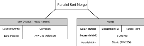
   Figure 8: Parallel Sort Merge Overview

   Fork Function: For the implementation of the fork function for the sorting problem, we have implemented a data parallel version based on AVX-256 Quicksort [5] and a thread and data sequential implementation of Combsort [16]. In this phase the algorithm focuses on partitioning the whole data set and applies to those partitions the designated local sort algorithm. The whole array is partitioned to be sorted according to a given block size. Jobs are assigned to each partition for local sorting. To ensure spatial locality, sub partitions are consecutively stored in tightly packed arrays. Each thread owns the memory region allowing independent read and write access, and thus ensuring concurrent sort of all blocks. A good first estimate for the block size is the size of the L2 cache.

   Join Function. After all partitions are sorted locally, each partition is merged pairwise iteratively until no more partition pairs are found. During the merging step, ensure that the sort order of the combined array is maintained. To make this step parallel we merge two adjacent partitions per thread. This individual merge thread can benefit from SIMD registers as well. We take the AVX2-based merge operators (bitonic sort network) from [3] and adapt it for 32-bit integer values as well. We also implement a sequential merge function for the basis of calculating achieved speedup. To ensure no bottlenecks occur due to dynamic memory management we pre-allocate the final sorted list twice for double buffering. We alternate between those two buffers at each merge level such that at no point do we require dynamic allocation for storing merge results. Each thread has exclusive access to their memory ranges ensuring parallel writes.

2. Instances: Parallel Sort Merge Join, Unique Filter, Id+Object Sort.

   As mentioned before, the parallel sort merge join instance implements the algorithm described in [3]. It is structured similar to the parallel sort instance, but since the input consists of two arrays to be joined according to some join key, now each thread holds a range partition, allowing local joins between the two locally sorted fact arrays to be performed. Further instances include a parallel sort unique filter, where the join step performs a modified merge operation filtering for unique values. This unique filter algorithm is used primarily in derivation trees (see Section 2.4) for deduplication of inferred facts. Finally, a fork-join instance for sorting objects, where arbitrary objects are sorted according to their associated integer id by swapping the same index values in the corresponding arrays. In this instance, the join operation is identical to the parallel sort, but the fork operation includes the extra swap operations for the object arrays. This fork-join instance is heavily used for sort keys in Section 2.3.1 and column-based join result structures, where the object arrays correspond to the individual columns.

2.4 Derivation Trees

The final component to discuss is the derivation tree concept, dealing with design chokepoints parallelism and lazy evaluation in the context of fact inference. The motivation for this component is based on (P2), as having the ability to filter out facts that are tied to inactive rules is beneficial for overall fact processing performance. In order to do so we need to define the queries that are in effect: active rules. We do this by building a rule hierarchy that maps the fact type dependencies between the rules. If the query does not necessitate certain types, then rules with those types can be excluded from processing (passed to the island processing component). A derivation tree is based on the strong typing property of each fact (see Definition 1) in order to structure the flow of inference (see Figure 9). Each node within this tree maintains the resulting data type and maps to it all of the conditions that map to that data type. The resulting data type is the <fact type> being inserted in the action part of a rule.

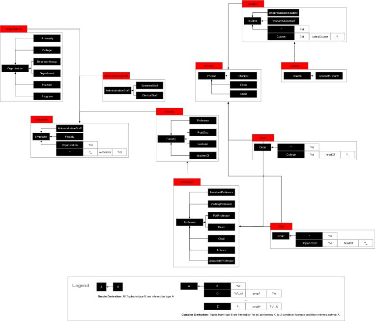
Figure 9: Derivation Tree

2.4.1 Parallel Execution using Derivation Trees

One of the benefits the derivation tree can realize is the identification of concurrent writing opportunities. Since the underlying data structure responsible for storing facts are the rank 1 indices, combined with facts’ strongly typed property – and thus being stored separately – it becomes possible to pipeline the index modification per <fact type>. The driving factor is the <fact type>, which is a meta data associated to the rule action. The top-down approach is used when processing derivation trees. Starting from level 0 root nodes, representing the rules that have no incoming edges (i.e. no rules are defined that result in derivation of this fact type), rule processing is done by grouping them by their resulting fact type, submitting each group to the job system for parallel execution. Each group is then processed sequentially inside the assigned thread. By doing so the rank 1 indices are modified consistently as each thread owns the memory range associated to that fact type. The levels are followed and each rule group is processed in the same fashion recursively until all levels are traversed. Algorithm 2 illustrates this parallel execution method using derivation trees. Note that in Line 7 the sort keys are re-initialized after each derivation tree level, to take into consideration any new cardinality updates due to any newly inferred facts (or deletions). Thus after each update the join order is optimized, given new data.

Input:

1          $deriv\_trees$ - derivation trees from all rules

2 Begin

3

4w $\leftarrow$ worker_threads_init();

5 foreach  $level$ in $deriv\_trees.levels()$  do

6       // out_group holds rules having write access to the same rank 1 index

7       // island construction (see Phase 1+2 from Algorithm 1) + associated sort_key encoding

8       islands $\leftarrow$ build_sort_keys(level.rules());

9       sort(islands by sort_keys grouped by rule);

10       foreach  $out\_group$ in $level.out\_groups()$  do

11             job $\leftarrow$ Job();

12             foreach  $rule$ in $out\_group.rules()$  do

13                   // island_sort_key_eval is simliar to Algorithm 1, excluding Phase 1+2 and any sort logic on the islands array. islands[$rule$] holds the pre-sorted island array for that rule.

14                   job.add(island_sort_key_eval, islands[$rule$]);

15            w.add(job);

16      w.start();

17       w.join();

18w.delete();

Algorithm 2 Parallel Rule Evaluation (sort keys)

2.4.2 Lazy Rule Execution

Drools [28] has shown the underlying problem of the forward chaining inference approach: all rules are followed leading to fact derivations that are not always necessary, leading to time wasted on unnecessary fact processing. Combined with Rete’s memoizing property, the problem is magnified due to caching unnecessary facts. To tackle this issue, the derivation tree is used to identify rules that are not required to be executed. In order to do so we distinguish rule nodes between derivation rules and queries. The distinction lies in whether there is an action associated to the rule that modifies facts. The existence of such actions signals the rule to be a derivation rule, and a query otherwise. Stated differently, leaf nodes in the derivation trees represent queries, and nodes with children represent derivation rules. The idea is to pre-define together with the flow of derivation rules the queries that are intended to be executed. These usually represent standard queries that are necessary for already known analysis tasks. These rules are then put together to create the derivation trees. When new queries are added while the Hiperfact system is running (e.g. ad-hoc queries), inactive derivation rules may become active to cover the new query. This process happens naturally as the derivation trees are rebuilt any time rules are modified. Following the derivation trees in a bottom-up fashion starting from leaf nodes (queries) allows us to identify inactive rules (see Definition 11). Derivation Rules where $RT(r)=\texttt{DERIVATION\_RULE}\wedge AR(r)=\texttt{false}$ can be skipped for processing as they do not depend on any queries.

Definition 10

[Rule Type] We define the rule type function RT accepting a rule as parameter (see Definition 3) as:

$$\texttt{RT}(r)=\begin{cases}\texttt{DERIVATION\_RULE},&\text{if }\texttt{children}(r)>0\\ \texttt{QUERY},&otherwise\end{cases}$$

children is a function returning the number of rule nodes that will be executed next according to the derivation tree. A rule node $c$ is a child of another rule $p$ when $c$ holds a
<fact type> in any of its conditions that is marked being modified in $p.action$.

Definition 11

[Active Rule] To determine whether a given Rule r is active, and thus needs to be evaluated, we define AR accepting, as parameter, a rule as follows:

$$\texttt{AR}(r)=\begin{cases}\texttt{true},&\exists x\in children(r),\texttt{AR}(x)\vee\texttt{RT}(x)=\texttt{QUERY}\\ \texttt{false},&otherwise\end{cases}$$

A rule is marked as active when a rule of type QUERY is on its path (i.e. from the leaf to the root node).

2.4.3 Recursive Execution of Derivation Trees

As derivation trees could by cyclic, where root nodes link to children nodes, the actual execution outlined in Section 2.4.1 needs to be repeated until a fixpoint is reached, i.e., where no new facts are inferred. Doing so might lead to facts that have been previously inferred. As such, an efficient deduplication operation of facts needs to be employed to be viable. We use the parallel unique filter discussed in Section 2.

3 Experimental Evaluation

In this section we discuss the experimental evaluation to observe the effectiveness of the introduced components and thus also the Hiperfact architecture. The primary measurements are the run-time performance metrics: data set loading time, fact inference time, and query time. Secondary measures are tracked as well for observing the last level (LL) and L1 CPU cache miss rate and the instructions per cycle. A high number of instructions executed per cycle, combined with a lower cache miss rate is indicative of a well-performing implementation, but these secondary measurements are tracked over the whole implementation and cannot pinpoint the individual components’ performance in that regard. For the primary metrics, we can show the complete breakdown of the total run-time.

Figure 10: Component Evaluation Overview

Figure 10 shows what aspects within the individual Hiperfact engine components are configurable and thus affect the final performance. Table 1 highlights the acronyms each of those configurations are mapped to, which will be referred to from this point on. For the rank 1 index, notable configurations are the different backend implementations (AI,HI,LPIM,LPID) responsible for fact storage and retrieval, which have been touched on in Section 2.2.

For the query-focused island processing we have different join algorithms: hash join (HJ) and parallel sort merge join (MJ), briefly mentioned in Section 2.3.2. For performing the inter fact join rank 1 index lookup (RNL) there are two: (AR) performing a rank $<$ 3 lookup for each inter-island condition with variables mapped from the now known join results table before joining with the target island and (DR) which is the default RNL operation without consideration of the existing join results to join with the next island. Furthermore, for the island processing component, we distinguish between a columnar (CR) and row-based (RR) data structure for storing intermediate join results. For the inference-focused derivation tree component, we have configurations for parallel (PR) vs sequential (SF) derivation tree node processing, and the related parallel (PW) vs sequential (SW) index write approaches. These have been discussed in Section 2.4.1. Finally, configurations exist for applying a unique filter on newly inferred facts, which might be already inferred at a previous inference loop. To discover such occurrences we employ a parallel sort merge based (SU) vs a hash table based (HU) unique filter.

Acronym	Description
Rank 1 Index
AI	3-level Sparse Array Index
HI	Hashtable Index
LPIM	Array Linked Pages Index + Memory Pool
LPID	Array Linked Pages Index + Dynamic Memory
Island Processing
HJ	Inter/Intra-Fact Hash Join
MJ	Inter/Intra-Fact Parallel Sort Merge Join
AR	Adapted RNL
DR	Default RNL
CR	Columnar Intermediate Join Results
RR	Row-based Intermediate Join Results
Derivation Trees
PF	Parallel Node Level Queries
SF	Sequential Node Level Queries
PW	Parallel Index Write
SW	Sequential Index Write
SU	Parallel Sort Merge Unique Filter
HU	Hashtable Incremental Unique Filter
Configurations
$\text{Hiperfact}_{\texttt{infer1}}$	LPIM+HJ/AR/CR+PF/PW/SU
$\text{Hiperfact}_{\texttt{query1}}$	AI+MJ/AR/CR+PF/PW/SU

Table 1: Hiperfact configurations

From several runs we have two pre-configured instances of Hiperfact: infer1 and query1. The former focuses on inference workloads and uses a memory pooled array linked pages (LPIM) rank 1 index, hash joins (HJ) for the join operation using the adapted RNL (AR) approach with columnar join result storage (CR) for island processing, and parallel derivation tree node processing for read (PF), parallel index writing (PW) together with a parallel sort merge unique filter (SU) for uniqueness checks. The query1 preset differs in that the rank 1 index backend employs the three-level sparse array index (AI instead of LPIM). Experimental Setup. For the experiments we used different machine setups. Due to space reasons, we will only include the inference and query benchmarks, for which we used a physical system running an AMD Ryzen 9 2950X @3.5GHz (16 Cores) CPU with 64GB of RAM having L1 and L2 cache sizes of 512KB and 8MB respectively.

3.1 Benchmarks

With the configurations defined, we run both inference focused benchmarks based on LUBM [13] and WordNet [24], as well as query focused benchmarks as specified in OpenRuleBench [22]. We also run existing engines to compare the run-time performance. Each engine+data set pair is executed 4 times, where the primary and secondary metrics are tracked. The secondary perf metrics: instructions per cycle, LL cache miss rate, and L1 Data cache miss rate are tracked using the Linux perf tool. We verify that each engine’s run-time performance is not negatively affected due to monitoring under perf by an additional run of that engine+data set pair outside of perf. In the case where a benchmark script exists (Inferray), we explicitly use the command that script calls and execute it under perf to track the metrics. The first run is not tracked, allowing the caches to be primed, and the subsequent 3 runs are then tracked and the average metrics are reported in tables 2, 3 for inference and tables 4, 5 for query focused benchmarks respectively.

		Time Elapsed (in sec)
	Load	Inference	Query
LUBM1
RDFox	0.101	0.038	0.002
Inferray	0.42	0.168	N/A
$\text{Hiperfact}_{\texttt{infer1}}$	0.544	0.0398	0.0021
$\text{Hiperfact}_{\texttt{query1}}$	0.0542	0.0295	0.0015
LUBM50
RDFox	5.453	0.646	0.152
Inferray	22.959	1.632	N/A
$\text{Hiperfact}_{\texttt{infer1}}$	3.9	0.765	0.104
$\text{Hiperfact}_{\texttt{query1}}$	3.485	0.829	0.082
LUBM100
RDFox	9.210	1.291	0.314
Inferray	40.645	3.150	N/A
$\text{Hiperfact}_{\texttt{infer1}}$	7.342	1.448	0.200
$\text{Hiperfact}_{\texttt{query1}}$	6.839	1.573	0.149
$\text{Hiperfact}_{\texttt{infer1}}$+HU	7.412	3.363	0.203
Hiperfact (HI+HJ/DR/RR+SF/SW/HU)	7.778	13.491	0.228
WordNet
RDFox	1.093	0.2378	N/A
Inferray	4.126	0.475	N/A
$\text{Hiperfact}_{\texttt{infer1}}$	3.75	0.1318	N/A

Table 2: LUBM Inference+Query Time Elapsed (Average Values of 3 Runs)

		perf metrics
	Instr./cycle	LL Cache Miss(%)	L1D Cache Miss(%)
LUBM1
RDFox	1.823	12.39%	0.81%
Inferray	1.20	20.14%	5.17%
$\text{Hiperfact}_{\texttt{infer1}}$	1.213	10.96%	6.46%
$\text{Hiperfact}_{\texttt{query1}}$	1.62	8.295%	5.42%
LUBM50
RDFox	1.543	12.31%	3.49%
Inferray	1.626	13.26%	2.10%
$\text{Hiperfact}_{\texttt{infer1}}$	2.013	10.52%	3.31%
$\text{Hiperfact}_{\texttt{query1}}$	1.61	12.904%	3.15%
LUBM100
RDFox	1.353	13.38%	3.77%
Inferray	1.506	13.50%	2.11%
$\text{Hiperfact}_{\texttt{infer1}}$	1.796	8.58%	2.92%
$\text{Hiperfact}_{\texttt{query1}}$	1.892	11.05%	2.88%
$\text{Hiperfact}_{\texttt{infer1}}$+HU	1.74	18.412%	2.91%
Hiperfact (HI+HJ/DR/RR+SF/SW/HU)	2.68	4.083%	20.98%
WordNet
RDFox	N/A	N/A	N/A
Inferray	1.46	16.81%	2.88%
$\text{Hiperfact}_{\texttt{infer1}}$	1.15	16.44%	5.17%

Table 3: LUBM Inference+Query perf metrics (Average Values of 3 Runs)

Inference Benchmarks (cf. Table 2 and Table 3) The LUBM benchmarks are scaled from 100k (LUBM1), 10M (LUBM50) to 17M (LUBM100) triples for the initial data set. WordNet has a data size of nearly 2M triples. Using the RDFS-Plus rule set, new facts are inferred before the systems are ready to be queried using the query template provided by the LUBM benchmark. We compare our engine against two inference engines: Inferray [32] and RDFox [25]. The former is specialized for handling RDFS-Plus rulesets and is thus hard coded into the implementation, the latter allows the definition of the ruleset using a datalog-like language as input. As RDFS-Plus can be seen as meta rules that initializes the concrete rules from the given fact types, we have implemented those instantiated rules directly as rules for the Hiperfact engine. We argue that this is an acceptable approach allowing us to proceed with the evaluation without having a concrete language parser and rule generator in place. The focus of this evaluation is how fast these rules are executed for the purpose of fact inference. We plan to add a Datalog parser at a later point.

As for the overall result, Hiperfact performs well against the compared systems. Regarding the time for loading triples, the sparse array index (AI) consistently performs better than the array linked page indices (LPIM, LPID) and scales better compared to RDFox and Inferray. The load performance anomaly in the WordNet data set can be explained due to the reverse declaration of types. Whereas the data type is usually declared first for a given object, in WordNet, this is done in the end, thus requiring a buffering process to hold the incomplete fact while the type is yet to be declared. The extra memory allocation required to do so is reflected in the lower loading time for this specific data set. One approach to improve this behaviour is to introduce a memory pool of pre-allocated triples to hold those temporary triples. In regards to inference performance, RDFox’s [25] concurrent core data structure becomes evident, as the increase in number of facts to be inferred widens the gap in performance in their favor compared to Inferray and Hiperfact. Hiperfact’s current rank 1 indices do not have a concurrent core implementation which would allow full write access to the index from multiple worker threads. Despite that, we were still able to exploit several parallelization points implemented via PF and PW. In PF we used the derivation tree to identify which nodes are independent of each other, allowing parallel querying of rule conditions leading to positive rule activations. In PW we then group these facts by their data type to be processed concurrently, as the indices allow concurrent write access per data type. This is reflected in the good scaling behaviour, similar to RDFox’s but slightly worse, using the infer1 configuration tuned for inference.

For Inferray, we were not able to reproduce their reported [32] benchmark behaviour, using the benchmark supplied by the authors^, . The reason seems to be the inaccurate reporting of the benchmark numbers when running the Inferray engine using their benchmark framework, compared with the numbers extracted from the log that is generated when the Inferray engine is executed. By default, 5 iterations are executed and the average of those 5 runs is claimed to be reported. By investigating the logs, we came to the conclusion that the best of the 5 runs are reported, which is always the last run. Furthermore, as the iteration number increases, the loop time improves by a consistent 10% to 38% depending on the data set. And since only the last iteration counts, the best time is being logged for the benchmark, which is misleading as in order to achieve that number, the effort of the previous 4 iterations needs to be included as well. Due to the consistent improvement in loop time after each iteration, even an average of those numbers leads to an inaccurate measure of total effort. Since no other engine under evaluation behaves this way (improved time after subsequent iteration), combined with the fact that we need to run all engines under perf to track secondary measures, and that Inferray itself does not show this incremental improvement behaviour when run with iteration number of 1 but 5 times, we do exactly that: run the benchmark program with an iteration number of 1 and follow the tracking methodology outlined in the beginning of this section using the reported inference times from the log Inferray generates.

	Time Elapsed (in sec)
	Load	Query
Mondial
RDFox	0.133	2.704
Hiperfact (LPIM+HJ/AR/CR)	0.155	0.000418
Hiperfact (LPIM+HJ/DR/CR)	0.154	0.00159
Hiperfact (LPIM+HJ/AR/RR)	0.156	0.000575
Hiperfact (LPIM+MJ/AR/CR)	0.154	0.000401
Hiperfact (LPID+HJ/AR/CR)	0.125	0.000482
Hiperfact (AI+HJ/AR/CR)	0.126	0.000395
Hiperfact (AI+MJ/AR/CR)	0.127	0.000354
Hiperfact (AI+HJ/AR/RR)	0.123	0.000569
Hiperfact (AI+HJ/DR/CR)	0.130	0.000900
DBLP
RDFox	0.820	0.033
Drools	1.887	1.116
XSB	40.149	1.126
Hiperfact (LPIM+HJ/AR/CR)	1.458	0.0018
Hiperfact (LPIM+HJ/DR/CR)	1.435	0.0231
Hiperfact (LPIM+HJ/AR/RR)	1.522	0.0027
Hiperfact (LPIM+MJ/AR/CR)	1.505	0.0016
Hiperfact (LPID+HJ/AR/CR)	1.453	0.0024
Hiperfact (AI+HJ/AR/CR)	1.403	0.0016
Hiperfact (AI+MJ/AR/CR)	1.506	0.0013
Hiperfact (AI+HJ/AR/RR)	1.476	0.0024
Hiperfact (AI+HJ/DR/CR)	1.425	0.0093
Hiperfact (AI+MJ/DR/CR)	1.505	0.0241

Table 4: OpenRuleBench Query Time Elapsed Results (Average Values of 3 Runs)

		perf metrics
	Instr./cycle	LL Cache Miss(%)	L1D. Cache Miss(%)
Mondial
RDFox	1.633	20.48%	8.62%
Hiperfact (LPIM+HJ/AR/CR)	1.353	10.62%	1.42%
Hiperfact (LPIM+HJ/DR/CR)	1.373	9.70%	1.45%
Hiperfact (LPIM+HJ/AR/RR)	1.386	10.24%	1.57%
Hiperfact (LPIM+MJ/AR/CR)	1.433	10.28%	1.52%
Hiperfact (LPID+HJ/AR/CR)	1.273	10.96%	1.49%
Hiperfact (AI+HJ/AR/CR)	0.753	26.80%	1.65%
Hiperfact (AI+MJ/AR/CR)	0.793	27.20%	1.65%
Hiperfact (AI+HJ/AR/RR)	0.863	19.87%	1.64%
Hiperfact (AI+HJ/DR/CR)	0.683	34.62%	1.70%
DBLP
RDFox	1.033	22.53%	2.31%
Drools	1.086	22.98%	4.88%
XSB	1.48	3.98%	3.86%
Hiperfact (LPIM+HJ/AR/CR)	1.463	21.26%	3.29%
Hiperfact (LPIM+HJ/DR/CR)	1.41	21.19%	3.31%
Hiperfact (LPIM+HJ/AR/RR)	1.48	21.18%	3.06%
Hiperfact (LPIM+MJ/AR/CR)	1.47	20.63%	3.00%
Hiperfact (LPID+HJ/AR/CR)	1.32	21.87%	3.42%
Hiperfact (AI+HJ/AR/CR)	1.23	26.89%	3.86%
Hiperfact (AI+MJ/AR/CR)	1.24	26.40%	3.70%
Hiperfact (AI+HJ/AR/RR)	1.23	27.34%	3.61%
Hiperfact (AI+HJ/DR/CR)	1.25	27.12%	3.69%
Hiperfact (AI+MJ/DR/CR)	1.38	22.83%	3.97%

Table 5: OpenRuleBench Query perf metrics (Average Values of 3 Runs)

Query Benchmarks (cf. Table 4 and Table 5) In terms of loading time, dynamic memory allocation configurations (AI,LPID) win due to the overhead of pre-allocating memory pools before they are required. Default RNL (DR) Lookup in all configurations are not interesting in terms of island processing as unnecessary facts are fetched that are joined during intra- as well as inter-fact joins. The adapted RNL fetches individual facts to be joined based on the actual values already in the join result buffer. The sparse array index is preferred for querying as Rank 1 Lookups (R1L) can simply take the pointer to the index holding required facts without having to copy elements around. RDFox seems to stall the least and exhibits the highest instructions per cycle. In this regard the Linked pages Index (LPIM/LPID) fare better compared to the sparse array index (AI) both in terms of less stalled instructions and better L2/L1 cache utilization. Having pre-allocated pages ready to be claimed by the index is beneficial for island processing. Another point is that less abrupt calls to dynamic memory allocation are needed leading to less copying of facts to accomodate the bigger buffer for holding intermediate results. The degraded query performance for RDFox in the mondial data set seems to be due to a cross product between the two classes to be joined. The used academic license version of RDFox might not have a full SPARQL query optimizer to perform efficient joins. XSB uses the L2 cache the most efficient. Regarding the difference in RNL lookup variations (AR vs DR), it is clear that AR is advantageous when the join result leads to a smaller number of lookups, which is the case for the mondial and dblp data sets. In the case where AR is not selective, then the individual rank $<$ 3 lookups will perform worse than a singular RNL lookup before the actual join, due to non-efficient usage of the CPU caches as multiple random memory locations are visited (in the AR case) compared to one consecutive array to be filtered (in the DR case). In conclusion, query execution performance is best achieved using a three-level sparse array index (AI) for rank 1 indices, combined with a parallel sort merge join (MJ), adapted RNL (AR) and column-oriented join result (CR) data structure in the island processing component.

4 Related Work

Inferray [32] follows the general forward chaining inference approach from Rete and addresses problem (4) through the use of tightly packed arrays and problem (1) by never storing intermediate results. Since the focus of Inferray is to perform inference in the Resource Description Framework (RDF) context, it implements specialized rules to solely cover that domain. In most cases, these rules handle equivalence between fact types, neither requiring complex pattern matching logic involving any of LIMIT, ORDER BY, JOIN nor aggregation functions. Another aspect to consider is the intended workflow when employing Inferray. The design is to perform the inference with the complete fact set preloaded and after materializing all inferred facts subsequently executing queries on the final data set. Any newly added facts after materialization will trigger a complete inference process of the whole data set from scratch. This limits interactive exploration of the data set.

Stylus [14] focuses on improved pattern matching performance (of SPARQL queries) by introducing strong typing capabilities during the query optimization process. It works independently of any inference approach and solely focuses on query execution. The assumption here is that the inferred facts are all pre-materialized on which the Stylus algorithm then runs the queries. It claims to use the Inferray approach for that purpose.

[14] divides facts by their entity type, avoiding unnecessary joins. In our work, we extend the triple structure by additional dimensions, namely to namespace facts via strong typing (see Definition 1). Only facts within the explicitly queried namespace are candidates for joining. Additionally, their approach converts all triple components independent of their type to an internal id for processing. In contrast, in our approach we further distinguish each data type and their relevant natural compression technique.

[12] analyses SPARQL queries and performs join re-ordering by analysing characteristic pairs to identify foreign relationships (one-to-many, many-to-many). This information is used to gain better join result estimation and order the stars comprising the query. We do not use characteristic pairs to identify foreign relationships, but use the underlying index information (rank-1 indices), and calculate the aggregated sums for conditions and finally islands to get good lookup and join estimates. The islands are processed in that order to keep the intermediate results as small as possible. Furthermore we use thread as well as data parallelism to further increase the performance of joins. The concept of stars in this work corresponds to the islands in our approach.

[26] focuses on the querying aspect and performs a query optimization step for structuring fact processing in an optimized manner. Similar to our island processing approach, it identifies islands that can be processed independently and processes these islands in parallel using a mixed CPU-GPU approach with the cost of maintaining all island results in memory before performing a final join. Following the 7, the islands are identified as: S1 = (((STORE_SALES JOIN CUSTOMER) JOIN DATE) JOIN INVENTORY), S2 = (STORE_RETURNS JOIN CUSTOMER), S3 = (CATALOG_SALES JOIN CUSTOMER).

5 Conclusion and Future Work

In this paper, we introduced the Hiperfact architecture, its components and algorithms that deal with both inference and querying of triple structured facts, that is common in RDF. The derivation tree component tackles the challenges evident in inference tasks: deduplication of inferred facts that already exist through the use of an optimized data and thread parallel sort and merge unique filter, lazy evaluation of inference rules that are only processed when associated queries exist. The island processing component, combined with the rank 1 index component and join result data structures and algorithms tackle the challenge of query optimization for fast retrieval of facts. This is achieved by implementing different rank 1 index backends following a common API to observe the behaviour of different array-based fact indices as well as implementing row-based and column-based intermediate join structures. The main challenge tackled in the island processing component is finding an efficient join order through the use of cost estimation derived from cardinalities in the rank 1 index. Furthermore the strong typing of facts, allows for natural parallelization for write and read access in the derivation tree component, as well as in the island processing component. All components strive to use the CPU caches (L1/L2) as efficiently as possible by proper aligning of fact data in the rank 1 index component and the join result data structures.

Hiperfact is slightly less performant regarding inference compared to RDFox, but comfortably beats Inferray. In the issues query optimization and execution Hiperfact’s island processing and derivation tree components show a concrete advantage over the competition. Future work for Hiperfact includes dynamic caching of rank 2 and 3 query results, allowing fine grained result among queries (including rule conditions), complex data types such as arrays and dictionaries in the value part of a fact allowing for modeling of complex data structures, type-based compression in the column-based join structures as well as in the rank 1 index to allow for more efficient storage and later retrieval.

References

- [1] Abadi, D., Madden, S., Ferreira, M.: Integrating compression and execution in column-oriented database systems. In: Proceedings of the 2006 ACM SIGMOD International Conference on Management of Data. pp. 671–682. SIGMOD ’06, ACM, New York, NY, USA (2006), http://doi.acm.org/10.1145/1142473.1142548
- [2] Aref, M.M., Tayyib, M.A.: Lana-match algorithm: A parallel version of the rete-match algorithm. Parallel Comput. 24(5-6), 763–775 (Jun 1998), http://dx.doi.org/10.1016/S0167-8191(98)00003-9
- [3] Balkesen, C., Alonso, G., Teubner, J., Özsu, M.T.: Multi-core, main-memory joins: Sort vs. hash revisited. Proc. VLDB Endow. 7(1), 85–96 (Sep 2013), https://doi.org/10.14778/2732219.2732227
- [4] Blanas, S., Li, Y., Patel, J.: Design and evaluation of main memory hash join algorithms for multi-core cpus. pp. 37–48 (01 2011)
- [5] Bramas, B.: Fast Sorting Algorithms using AVX-512 on Intel Knights Landing (Apr 2017), https://hal.inria.fr/hal-01512970, working paper or preprint
- [6] Brant, D.A., Grose, T., Lofaso, B., Miranker, D.P.: Effects of database size on rule system performance: Five case studies. In: Proceedings of the 17th International Conference on Very Large Data Bases. p. 287–296. VLDB ’91, Morgan Kaufmann Publishers Inc., San Francisco, CA, USA (1991)
- [7] Drepper, U.: What every programmer should know about memory (2007)
- [8] Erling, O., Averbuch, A., Larriba-Pey, J., Chafi, H., Gubichev, A., Prat, A., Pham, M.D., Boncz, P.: The ldbc social network benchmark: Interactive workload. In: Proceedings of the 2015 ACM SIGMOD International Conference on Management of Data. p. 619–630. SIGMOD ’15, Association for Computing Machinery, New York, NY, USA (2015), https://doi.org/10.1145/2723372.2742786
- [9] Fabret, F., Régnier, M., Simon, E.: An adaptive algorithm for incremental evaluation of production rules in databases. In: Proceedings of the 19th International Conference on Very Large Data Bases. p. 455–466. VLDB ’93, Morgan Kaufmann Publishers Inc., San Francisco, CA, USA (1993)
- [10] Faye, D., Curé, O., Blin, G.: A survey of rdf storage approaches. ARIMA Journal 15, 11–35 (01 2012)
- [11] Forgy, C.: Rete: A fast algorithm for the many patterns/many objects match problem. Artif. Intell. 19(1), 17–37 (1982)
- [12] Gubichev, A., Neumann, T.: Exploiting the query structure for efficient join ordering in sparql queries. In: IN EDBT. pp. 439–450 (2014)
- [13] Guo, Y., Pan, Z., Heflin, J.: Lubm: A benchmark for owl knowledge base systems. Journal of Web Semantics 3(2), 158 – 182 (2005), http://www.sciencedirect.com/science/article/pii/S1570826805000132, selcted Papers from the International Semantic Web Conference, 2004
- [14] He, L., Shao, B., Li, Y., Xia, H., Xiao, Y., Chen, E., Chen, L.J.: Stylus: A strongly-typed store for serving massive rdf data. Proc. VLDB Endow. 11(2), 203–216 (Oct 2017), https://doi-org.uaccess.univie.ac.at/10.14778/3149193.3149200
- [15] Hill, E.F.: Jess in Action: Java Rule-Based Systems. Manning Publications Co., USA (2003)
- [16] Inoue, H., Taura, K.: Simd- and cache-friendly algorithm for sorting an array of structures. Proc. VLDB Endow. 8(11), 1274–1285 (Jul 2015), https://doi.org/10.14778/2809974.2809988
- [17] Jin, C., Carbonell, J., Hayes, P.: Argus: Rete + dbms = efficient persistent profile matching on large-volume data streams. vol. 3488, pp. 142–151 (05 2005)
- [18] Khadilkar, V., Kantarcioglu, M., Thuraisingham, B., Castagna, P.: Jena-hbase: A distributed, scalable and effcient rdf triple store. (01 2012)
- [19] Kim, M., Lee, K.S., Kim, Y., Kim, T., Lee, Y., Cho, S., Lee, C.G.: Rete-adh: An improvement to rete for composite context-aware service. International Journal of Distributed Sensor Networks 2014, 1–11 (04 2014)
- [20] Lang, H., Leis, V., Albutiu, M.C., Neumann, T., Kemper, A.: Massively Parallel NUMA-Aware Hash Joins, pp. 3–14 (01 2015)
- [21] Liang, S., Fodor, P., Wan, H., Kifer, M.: Openrulebench: An analysis of the performance of rule engines. In: Proceedings of the 18th International Conference on World Wide Web. p. 601–610. WWW ’09, Association for Computing Machinery, New York, NY, USA (2009), https://doi.org/10.1145/1526709.1526790
- [22] Liang, S., Fodor, P., Wan, H., Kifer, M.: Openrulebench: An analysis of the performance of rule engines. In: Proceedings of the 18th International Conference on World Wide Web. p. 601–610. WWW ’09, Association for Computing Machinery, New York, NY, USA (2009), https://doi.org/10.1145/1526709.1526790
- [23] Marr, S., Renaux, T., Hoste, L., Meuter, W.: Parallel gesture recognition with soft real-time guarantees. Science of Computer Programming 98 (04 2014)
- [24] Miller, G.A.: Wordnet: A lexical database for english. Commun. ACM 38(11), 39–41 (Nov 1995), https://doi.org/10.1145/219717.219748
- [25] Motik, B., Nenov, Y., Piro, R., Horrocks, I., Olteanu, D.: Parallel materialisation of datalog programs in centralised, main-memory rdf systems. In: Proceedings of the Twenty-Eighth AAAI Conference on Artificial Intelligence. p. 129–137. AAAI’14, AAAI Press (2014)
- [26] Nam, Y.M.N., Han, D.H., Kim, M.S.K.: Sprinter: A fast n-ary join query processing method for complex olap queries. In: Proceedings of the 2020 ACM SIGMOD International Conference on Management of Data. p. 2055–2070. SIGMOD ’20, Association for Computing Machinery, New York, NY, USA (2020), https://doi.org/10.1145/3318464.3380565
- [27] Nyman, L., Laakso, M.: Notes on the history of fork and join. IEEE Annals of the History of Computing 38(3), 84–87 (2016)
- [28] Proctor, M., Fusco, M., Sottara, D., Zimányi, T.: Reducing the Cost of the Linear Growth Effect Using Adaptive Rules with Unlinking and Lazy Rule Evaluation: Confederated International Conferences: CoopIS, C&TC, and ODBASE 2018, Valletta, Malta, October 22-26, 2018, Proceedings, Part II, pp. 592–601 (10 2018)
- [29] Riley, G.: Clips: An expert system building tool (1991)
- [30] Schmidt, K.U., Stühmer, R., Stojanovic, L., Anicic, D., Brelage, C., Etzion, O., Stojanovic, N.: Blending complex event processing with the rete algorithm (2008)
- [31] Sottara, D., Mello, P., Proctor, M.: A configurable rete-oo engine for reasoning with different types of imperfect information. IEEE Transactions on Knowledge and Data Engineering 22(11), 1535–1548 (2010)
- [32] Subercaze, J., Gravier, C., Chevalier, J., Laforest, F.: Inferray: Fast in-memory rdf inference. Proc. VLDB Endow. 9(6), 468–479 (Jan 2016), http://dx.doi.org/10.14778/2904121.2904123
- [33] Zhou, R., Wang, G., Wang, J., Li, J.: Runes ii: A distributed rule engine based on rete network in cloud computing. International Journal of Grid and Distributed Computing 7, 91–110 (12 2014)