Polarization and Belief Convergence of Agents in Strongly-Connected Influence Graphs

Abstract

We describe a model for polarization in multi-agent systems based on Esteban and Ray’s classic measure of polarization from economics. Agents evolve by updating their beliefs (opinions) based on the beliefs of others and an underlying influence graph. We show that polarization eventually disappears (converges to zero) if the influence graph is strongly-connected. If the influence graph is a circulation we determine the unique belief value all agents converge to. For clique influence graphs we determine the time after which agents will reach a given difference of opinion. Our results imply that if polarization does not disappear then either there is a disconnected subgroup of agents or some agent influences others more than she is influenced. Finally, we show that polarization does not necessarily vanish in weakly-connected graphs, and illustrate the model with a series of case studies and simulations giving some insights about polarization.

1 Introduction

Social networks facilitate the exchange of opinions by providing users with information from influencers, friends, or other users with similar or sometimes opposing views [4]. This may allow a healthy exposure to diverse perspectives, but it may lead also to the problems of misinformation and radicalization of opinions.

In social scenarios, a group may shape their beliefs by attributing more value to the opinions of influential figures. This cognitive bias is known as authority bias [23]. Furthermore, in a group with uniform views, users may become extreme by reinforcing one another’s opinions, giving more value to opinions that confirm their own beliefs; another common cognitive bias known as confirmation bias [3]. As a result, social networks can cause their users to become radical and isolated in their own ideological circle causing dangerous splits in society [4] in a phenomenon known as polarization [3].

There is a growing interest in the development of models for the analysis of polarization [16, 22, 27, 12, 10, 5, 21, 7, 13, 6, 25, 26, 15]. To our knowledge, however, the development of concurrency-based models for this phenomenon has been far too little considered. Since polarization involves non-terminating systems with multiple agents simultaneously exchanging information (opinions), concurrency models are a natural choice to capture the dynamics of polarization.

In fact, we developed a multi-agent model for polarization in [2], inspired by linear-time models of concurrency where the state of the system evolves in discrete time units (in particular, [24, 19]). In each time unit, the agents (users) update their beliefs (opinions) according to the underlying influence graph and the beliefs of their neighbors. The influence graph is a weighted directed graph describing connectivity and influence of each agent over the others. Two belief updates are considered. The regular belief update gives more value to the opinion of agents with higher influence, representing authority bias. The confirmation bias update gives more value to the opinion of agents with similar views. Furthermore, the model is equipped with a polarization measure based on the seminal work in economics by Esteban and Ray [11]. The polarization is measured at each time unit and it is $0$ if all agents achieve complete consensus about a given proposition. The contributions in [2] were of an experimental nature and aimed at exploring how the combination of interaction graphs and cognitive biases in our model can lead to polarization.

In the current paper we prove claims made from experimental observations in [2] using techniques from calculus, graph theory, and flow networks. We study meaningful families of influence graphs for which polarization eventually becomes zero (vanishes). In particular we consider cliques, strongly-connected, and balanced-influence graphs, and the belief update can be regular or with confirmation bias. We derive new properties not observed through experiments in [2] and state connections between influence and the notion of flow from network theory. Our results provide insight into the phenomenon of polarization, and are a step toward the design of robust computational models and simulation software for human cognitive and social processes. We therefore believe that FoSSaCS, whose specific topics include models for concurrent systems, would be an excellent venue for this work.

Main Contributions.

In this paper we establish the following theoretical results:

1. If the influence graph is strongly-connected then the agents’ beliefs converge to one value (i.e., they reach consensus), and polarization converges to zero.

2. For weakly-connected and influence-balanced influence graphs (each agent influences others as much as she is influenced) we give the value of belief convergence.

3. For clique influence graphs we determine the exact value of belief convergence and the time after which agents reach a given difference of opinion.

4. If polarization does not converge to zero then either there is a group disconnected from the rest, or there is an agent that influences others more than she is influenced.

5. Polarization does not necessarily converge to zero for weakly-connected graphs.

We also illustrate a series of case studies and simulations, uncovering interesting new insights and perhaps counter-intuitive characteristics of the phenomena. The code of the implementation of the model and simulations is provided in this paper. We discuss related work in Section 2. We introduce the model in Section 3, and present case studies and simulations in Section 4. The theoretical results are shown in Sections 5 and 6.

2 Related Work

As social networks have become ubiquitous, their wide-ranging effects on the world have motivated a great deal of research. Here we provide an overview of the range of relevant approaches to the problems we are considering, and put into perspective the novelty of our approach to the problem.

Polarization Polarization was originally studied as a psychological phenomenon in [18], and it was first rigorously and quantitatively defined by economists Esteban and Ray [11]. Their measure of polarization, discussed in Section 3, is influential, and is the one we adopt in this paper. Li et al.[16] were the first to model consensus and polarization in social networks. Like most other work, they did not quantify polarization, but focused on when and under what conditions a population reaches consensus.fancyline]Frank: Notice that in this paper that’s exactly what we do. Proskurnikov et al. [22] investigated the formation of consensus or polarization in social networks, but considered polarization as lack of consensus, rather than a phenomenon in its own right. Elder’s work [10] focuses on methods to avoid polarization, without using a quantitative definition of polarization. [5] and [21] measure polarization but purely as a function of network topology, rather than taking agents’ quantitative beliefs and opinions into account.

Formal Models Sîrbu et al. [27] use a model somewhat similar to ours, except that it updates probabilistically. They investigate the effects of algorithmic bias on polarization by counting the number of opinion clusters, interpreting a single opinion cluster as consensus, rather than directly measuring polarization itself. Leskovec et al. [12] develop simulated social networks and observe group formation over time. Their work is not concerned with a formal measure of polarization. [5] and [21] measure polarization but purely as a function of network topology, rather than taking agents’ quantitative beliefs and opinions into account. The models in [7] and [13] are closest to ours; however, rather than examining polarization and opinions, this work is concerned with the network topology conditions under which agents with noisy data about an objective fact converge to an accurate consensus, close to the true state of the world. This is related to our goals in the sense that agents who have converged to a consensus have a low level of polarization, but the problem of obtaining accurate information about the world through communication is different than our focus on changing opinions about an issue which does not have an objective, outside value.

Logic-based approaches Liu et al. [17] use ideas from doxastic and dynamic epistemic logics to qualitatively model influence and belief change in social networks. Christoff [6] develops several non-quantitative logics for social networks, concerned with problems related to polarization, such as information cascades. Seligman et al. [25, 26] introduce a basic “Facebook logic.” This logic is non-quantitative, but its interesting point is that an agent’s possible worlds are different social networks. This is a promising approach to formal modeling of epistemic issues in social networks. Hunter [15] introduces a logic of belief updates over social networks where closer agents in the social network are more trusted and thus more influential. While beliefs in this logic are non-quantitative, it includes a quantitative notion of influence between users.

3 Background: The Model

In this section we recall the polarization model introduced in [2]. We presuppose basic knowledge of calculus and graph theory [28, 8]. We divide the elements of our model into static and dynamic parts, described next.

3.1 Static elements of the model

Static elements of the model represent a snapshot of a social network at a given point in time. The model includes the following static elements:

• A (finite) set $\mathcal{A}=\{0,1,\ldots,n{-}1\}$ of $n\geq 1$ agents.

• A proposition $p$ of interest, about which agents can hold beliefs.

• A belief configuration $B{:}\mathcal{A}{\rightarrow}[0,1]$ s.t. each value $B_{i}$ is the instantaneous confidence of agent $i{\in}\mathcal{A}$ in the veracity of proposition $p$. The extreme values $0$ and $1$ represent a firm belief in, respectively, the falsehood or truth of the proposition $p$.

• A polarization measure $\rho{:}[0,1]^{\mathcal{A}}{\rightarrow}\mathbb{R}$ mapping belief configurations to real numbers. The value $\rho(B)$ indicates how polarized belief configuration $B$ is.

There are several polarization measures described in the literature. In this work we concentrate on the influential measure proposed by Esteban and Ray [11].

Definition 1 (Esteban-Ray polarization measure)

Consider a discrete set $\mathcal{Y}=\{y_{0},\allowbreak y_{1},\allowbreak\ldots,\allowbreak y_{k-1}\}$ of size $k$, s.t. each $y_{i}{\in}\mathbb{R}$. Let $(\pi,y){=}(\pi_{0},\allowbreak\pi_{1},\allowbreak\ldots,\allowbreak\pi_{k{-}1},\allowbreak y_{0},\allowbreak y_{1},\allowbreak\ldots,\allowbreak y_{k{-}1})$ be a distribution on $\mathcal{Y}$ s.t. $\pi_{i}$ is the frequency of value $y_{i}{\in}\mathcal{Y}$ in the distribution. W.l.o.g. we can assume the values of $\pi_{i}$ are all non-zero and add up to 1 (as in a standard probability distribution). The Esteban-Ray (ER) polarization measure is defined as

$$\rho_{\mathit{ER}}(\pi,y)=K\sum_{i=0}^{k-1}\sum_{j=0}^{k-1}\pi_{i}^{1+\alpha}\pi_{j}|y_{i}-y_{j}|,$$

where $K>0$ is a constant, and typically $\alpha\approx 1.6$.

The higher the value of $\rho_{\mathit{ER}}(\pi,y)$, the more polarized the distribution $(\pi,y)$ is. The measure captures the intuition that polarization is accentuated by both intra-group homogeneity and inter-group heterogeneity. Moreover, it assumes that the total polarization is the sum of the effects of individual agents on one another. The measure can be derived from a set of intuitively reasonable axioms [11], described in Appendix 0.B.

Note, however, that $\rho_{\mathit{ER}}$ is defined on a discrete distribution, whereas in our model a general polarization metric is defined on a belief configuration $B{:}\mathcal{A}{\rightarrow}[0,1]$. To properly apply $\rho_{\mathit{ER}}$ to our setup we need to convert the belief configuration $B$ into an appropriate distribution $(\pi,y)$ as expected by the measure. We can do this as follows. Given a number $k{>}0$ of (discretization) bins, define $\mathcal{Y}{=}\{y_{1},y_{2},\ldots,y_{k}\}$ as a discretization of the range $[0,1]$ in such a way that each $y_{i}$ represents the interval $y_{i}{=}\left[\nicefrac{{i}}{{k}},\nicefrac{{i+1}}{{k}}\right]$. Define, then, the weight $\pi_{i}$ of value $y_{i}$, corresponding to the fraction of agents having belief in the interval $y_{i}$, as $\pi_{i}{=}\nicefrac{{\left(\sum_{a\in\mathcal{A}}\mathbbm{1}_{y_{i}}\left(B_{i}\right)\right)}}{{|\mathcal{A}|}},$ where $\mathbbm{1}_{\mathcal{X}}\left(x\right)$ is the indicator function returning 1 if $x\in\mathcal{X}$, and 0 otherwise. Notice that in the particular case in which all agents in the belief configuration $B$ hold the same belief value, i.e., when there is consensus about the proposition $p$ under consideration, $\rho_{\mathit{ER}}$ produces 0.

3.2 Dynamic elements of the model

Dynamic elements of the model capture the information necessary to formalize the evolution of agents’ beliefs in the social network. Although these aspects are not directly used to compute the instantaneous level of polarization, they determine how polarization evolves. The dynamic elements of our model are the following:

• An influence graph $\mathcal{I}{:}\mathcal{A}{\times}\mathcal{A}{\rightarrow}[0,1]$ s.t., for all $i,j{\in}\mathcal{A}$, $\mathcal{I}(i,j)$, written $\mathcal{I}_{i,j}$, represents the influence of agent $i$ on agent $j$. A higher value means stronger influence. We shall often refer to $\mathcal{I}$ simply as the influence $\mathcal{I}$.

• A time frame $\mathcal{T}{=}\{0,1,2,\ldots\}$ representing the discrete passage of time.

• A family of belief configurations $\{B^{t}{:}\mathcal{A}{\rightarrow}[0,1]\}_{t{\in}{\mathcal{T}}}$ indexed by time steps s.t. each $B^{t}$ is a social network’s belief configuration w.r.t. proposition $p$ at time step $t{\in}\mathcal{T}$.

• An update function $\mu{:}B{\times}\mathcal{I}{\rightarrow}B$ mapping a belief configuration and an interaction graph to a new belief configuration. $B^{t+1}{=}\mu(B^{t},\mathcal{I})$ models the evolution of agents’ beliefs from time step $t$ to $t{+}1$ when their interaction is modeled by $\mathcal{I}$.

The definition of an update function depends on how agents incorporate new evidence into their reasoning. In this work the update function considers that the impact of agent $j$’s belief on agent $i$’s is proportional to the influence $\mathcal{I}_{j,i}$ of $j$ on $i$, and to the difference $B^{t}_{j}{-}B^{t}_{i}$ in their beliefs. The function then averages all influences on an agent to compute the corresponding belief update. This intuition is formalized next.

Definition 2 (Update function)

Let $B^{t}$ be a belief configuration at time step $t{\in}\mathcal{T}$, and $\mathcal{I}$ be an influence graph. The update function $\mu^{R}{:}B{\times}\mathcal{I}{\rightarrow}B$ is defined s.t. the updated belief configuration $B^{t+1}{=}\mu^{R}(B^{t},\mathcal{I})$ at time step $t{+}1$, for all agents $i$, is given by

$$B^{t+1}_{i}=\frac{1}{|\mathcal{A}|}\sum_{j\in\mathcal{A}}B^{t+1}_{i{\mid}j}~{},\quad\text{where}\quad B^{t+1}_{i{\mid}j}=B^{t}_{i}+\mathcal{I}_{j,i}\left(B^{t}_{j}-B^{t}_{i}\right)~{}$$

represents the influence of agent $j\in\mathcal{A}$ on agent $i$’s belief at time $t{+}1$ after both agents interact at time $t$. The value $B^{t+1}_{i}$ is agent $i$’s belief at time $t{+}1$, resulting from the weighted average of interactions with all agents at time $t$, in parallel.

Notice that the above update function models agents who incorporate equitably all evidence available, be it in favor or against a proposition, when updating their beliefs. Yet, influence graphs allow us to capture different intensities of authority bias [23], by which an agent gives more weight to evidence presented by some agents than by others. As a particular case, a proper setting of influence values can capture agents sensitive only to the contents of information, independent from its source.

4 Simulations and Motivating Examples

In this section we present several simulations of the evolution of beliefs and polarization in our model, employing various combinations of meaningful influence graphs and initial belief configurations. These examples provide insights that are captured as formal properties in Sec.5.

For the computation of the Esteban-Ray measure (Def. 1), we discretize the interval $[0,1]$ of possible belief values into 5 bins, each representing a possible general position w.r.t. the veracity of the proposition $p$ of interest: strong disagreement, $[0,0.20)$; mild disagreement, $[0.20,0.40)$; indifference, $[0.40,0.60)$; mild agreement, $[0.60,0.80)$; and strong agreement, $[0.80,1]$. We set parameters $\alpha{=}1.6$, as suggested by Esteban and Ray [11], and $K{=}1000$. In all definitions we let $\mathcal{A}{=}\{0,1,\ldots,n{-}1\}$, and $i,j{\in}\mathcal{A}$ be generic agents. Each simulation uses a set of $n{=}100$ agents (unless otherwise noted), and limits execution to a threshold of $T$ time steps, varying according to the experiment.

We consider the following initial belief configurations, depicted in Figure 1.

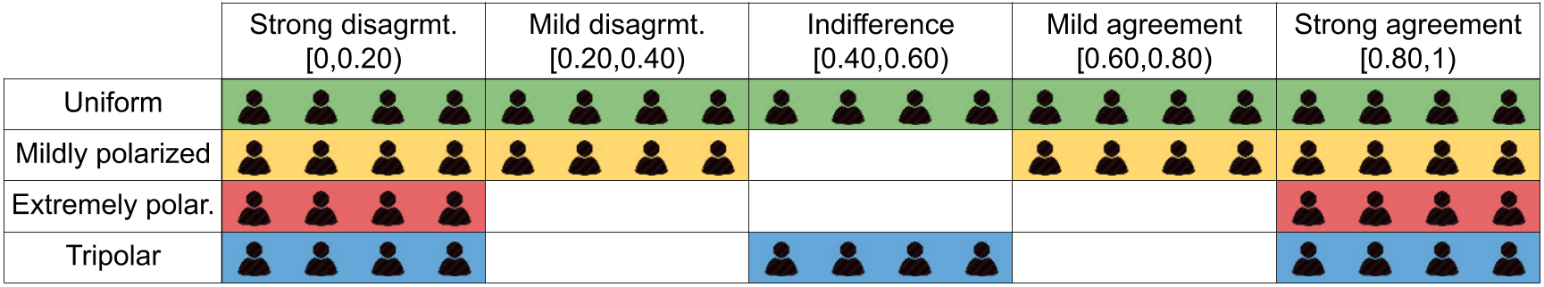
Figure 1: Depiction of different initial belief configurations used in simulations.

• A uniform belief configuration representing a set of agents whose beliefs are as varied as possible, all equally spaced in the interval $[0,1]$: $B^{0}_{i}{=}\nicefrac{{i}}{{(n{-}1)}}.$

• A mildly polarized belief configuration representing agents evenly split into two groups with moderately dissimilar inter-group beliefs compared to their intra-group beliefs: $B^{0}_{i}{=}\nicefrac{{0.8i}}{{n}}$, if $i{<}\lceil\nicefrac{{n}}{{2}}\rceil$; or $B^{0}_{i}{=}\nicefrac{{0.8i}}{{n}}{+}0.20$, otherwise.

• An extremely polarized belief configuration representing a situation in which half of the agents strongly believe the proposition, whereas the other half strongly disbelieve it: $B^{0}_{i}{=}\nicefrac{{0.4i}}{{n}}$, if $i{<}\lceil\nicefrac{{n}}{{2}}\rceil$; or $B^{0}_{i}{=}\nicefrac{{0.4i}}{{n}}{+}0.60$, otherwise.

• A tripolar configuration representing agents divided into three groups of similar size sharing similar beliefs: $B^{0}_{i}{=}\nicefrac{{0.60i}}{{n}}$, if $0{\leq}i{<}\lfloor\nicefrac{{n}}{{3}}\rfloor$; $B^{0}_{i}{=}\nicefrac{{0.60i}}{{n}}+0.20$, if $\lfloor\nicefrac{{n}}{{3}}\rfloor{\leq}i{<}\lceil\nicefrac{{2n}}{{3}}\rceil$; or $B^{0}_{i}{=}\nicefrac{{0.60i}}{{n}}+0.40$, otherwise.

As for influence graphs, we consider the following ones, depicted in Figure 2.

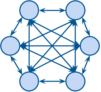
(a) Clique

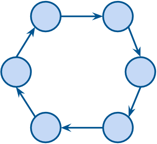
(b) Circular

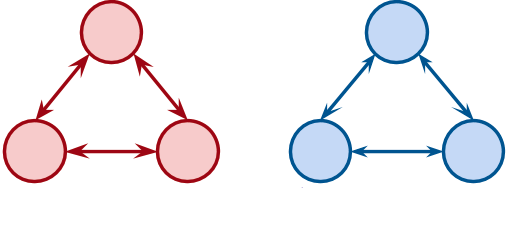
(c) Disconnected groups

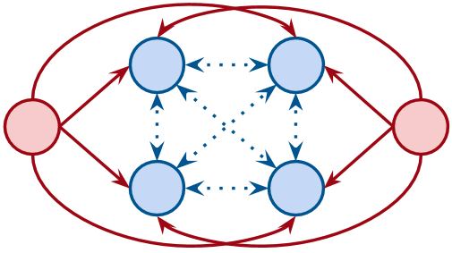
(d) Unrelenting influencers

Figure 2: The general shape of influence graphs used in simulations.

• A $C$-clique influence graph $\mathcal{I}^{\textit{clique}}$ (formalized in Def. 3 ahead), in which each agent influences every other with constant value $C=0.5$: $\mathcal{I}^{\textit{clique}}_{i,j}{=}0.5$, for every $i,j$. This represents the particular case of a social network in which all agents interact among themselves, and are all immune to authority bias.

• A circular influence graph $\mathcal{I}^{\textit{circ}}$ representing a social network in which agents can be organized in a circle in such a way each agent is only influenced by its predecessor and only influences its successor. This is a simple instance of a balanced graph (in which each agent’s influence on others is as high as the influence received, as in Def. 9 ahead), which is a pattern commonly encountered in some sub-networks. More precisely: $\mathcal{I}^{\textit{circ}}_{i,j}{=}0.5$, if $(i{+}1)\,\text{mod}\,n{=}j$; and $\mathcal{I}^{\textit{circ}}_{i,j}{=}0$, otherwise.

• A disconnected influence graph $\mathcal{I}^{\textit{disc}}$ representing a social network sharply divided into two groups in such a way that agents within the same group can considerably influence each other, but not at all agents in the other group: $\mathcal{I}^{\textit{disc}}_{i,j}{=}0.5$, if $i,j$ are both ${<}\lceil\nicefrac{{n}}{{2}}\rceil$ or both ${\geq}\lceil\nicefrac{{n}}{{2}}\rceil$, and $\mathcal{I}^{\textit{disc}}_{i,j}{=}0$ otherwise.

• An unrelenting influencers influence graph $\mathcal{I}^{\textit{unrel}}$ representing a scenario in which two agents (say, $0$ and $n{-}1$) exert significantly stronger influence on every other agent than these other agents have among themselves. More precisely: $\mathcal{I}^{\textit{unrel}}_{i,j}{=}0.6$ if $i{=}0$ and $j{\neq}n{-}1$ or $i{=}n{-}1$ and $j{\neq}0$; $\mathcal{I}^{\textit{unrel}}_{i,j}{=}0$ if $j{=}0$ or $j{=}n{-}1$; and finally $\mathcal{I}^{\textit{unrel}}_{i,j}{=}0.1$ if $0{\neq}i{\neq}n{-}{1}$ and $0{\neq}j{\neq}n{-}{1}$. This could represent, e.g., a social network in which two totalitarian media companies dominate the news market, both with similarly high levels of influence on all agents. The networks have clear agendas to push forward, and are not influenced in a meaningful way by other agents.

We simulated the evolution of agents’ beliefs and the corresponding polarization of the network for all combinations of initial belief configurations and influence graphs presented above. The results, depicted in Figure 3, will be used throughout this paper to illustrate some of our formal results. Both the Python implementation of the model and the Jupyter Notebook containing the simulations are available on Github [1].

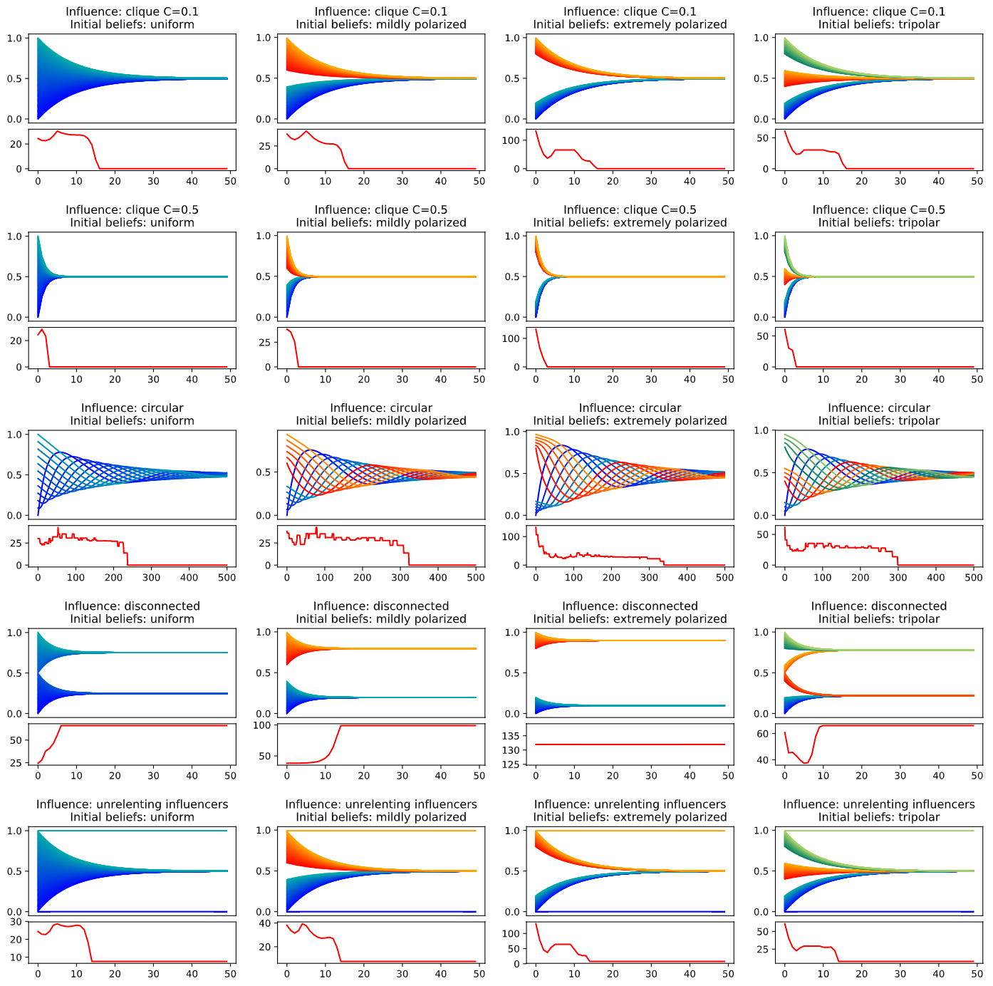
Figure 3: Simulations of the evolution of beliefs (upper part of each graph) and of polarization (lower part of each graph) under different initial belief configurations and influence graphs. In each graph the horizontal axis represents the discrete passing of time. Each row contains all graphs with the same influence graph, and each column all graphs with the same initial belief configuration. All simulations considered $n{=}100$ agents, with the exception of those regarding the circular influence graph, which used $n{=}12$ agents.

5 Consensus under Strongly-Connected Influence

Polarization eventually disappears if the agents asymptotically agree upon a common belief value for the proposition of interest; i.e., if they reach consensus. In our model this means that the polarization measure (Def.1) converges to zero if the limiting value of agent beliefs is the same as time approaches infinity.

In this section, the main and most technical of this paper, we consider meaningful families of influence graphs that guarantee consensus for all agents. We also identify fundamental properties of agents under this influence, as well as the time to achieve a given opinion difference and the actual value of convergence. We shall also relate influence with the notion of flow in flow networks.

5.1 Constant Cliques

We now introduce the notion of clique influence graph. It is meant to capture a scenario where all agents influence one another with the same value.

Definition 3 (Clique Influence)

Let $C$ be a real value in $(0,1].$ We say that the influence graph $\mathcal{I}$ is a $C$-clique if for all $i,j\in\mathcal{A}$ if $i\neq j$ then $\mathcal{I}_{i,j}=C.$

The following equations are immediate consequences of restricting Def.2 to $C$-cliques.

$$B^{t+1}_{i}\quad=\quad B^{t}_{i}+\frac{C}{\mid\mathcal{A}\mid}\sum_{j\in\mathcal{A}}\left(B^{t}_{j}-B^{t}_{i}\right)\quad=\quad B^{t}_{i}-CB^{t}_{i}+\frac{C}{\mid\mathcal{A}\mid}\sum_{j\in\mathcal{A}}B^{t}_{j}$$ (1)

The next definition identifies agents with extreme beliefs at a given time.

Definition 4 (Extreme Agents)

We say that an agent $i\in\mathcal{A}$ is maximal (minimal) at time $t$ if $B^{t}_{i}\geq B^{t}_{j}$ ($B^{t}_{i}\leq B^{t}_{j}$) for all $j\in\mathcal{A}$. An extreme agent at time $t$ is an agent that is maximal or minimal at time $t$.

An invariant property of extreme agents under clique influence is that they cannot become more extreme.

Proposition 1

If $\mathcal{I}$ is a $C$-clique and $i\in\mathcal{A}$ is maximal (minimal) at time $t$ then

1. $B^{t+1}_{i}\leq B^{t}_{i}$ ($B^{t+1}_{i}\geq B^{t}_{i}$).

2. $B^{t+1}_{i}<B^{t}_{i}$ ($B^{t+1}_{i}>B^{t}_{i}$) if there is $j\in\mathcal{A}$ such that $B^{t}_{j}\neq B^{t}_{i}.$

Proof

Let $i\in\mathcal{A}$ be maximal agent at time $t$. (1) We have $\sum_{j\in\mathcal{A}}\left(B^{t}_{j}-B^{t}_{i}\right)\leq 0.$ Hence from Eq.1, $B^{t+1}_{i}=B^{t}_{i}+\nicefrac{{C}}{{\mid\mathcal{A}\mid}}\sum_{j\in\mathcal{A}}\left(B^{t}_{j}-B^{t}_{i}\right)\leq B^{t}_{i}.$ (2) Assume $j\in\mathcal{A}$ with $B^{t}_{j}\not=B^{t}_{i}.$ Then $\sum_{j\in\mathcal{A}}\left(B^{t}_{j}-B^{t}_{i}\right)<0$ and thus, from Eq.1, $B^{t+1}_{i}=B^{t}_{i}+\nicefrac{{C}}{{\mid\mathcal{A}\mid}}\sum_{j\in\mathcal{A}}\left(B^{t}_{j}-B^{t}_{i}\right)<B^{t}_{i}.$ The cases when $i$ is minimal are similar. ∎

A distinguishing property for $C$-cliques is that extreme agents continue to be extreme. This property is a consequence of the following proposition.

Proposition 2 (Order Preservation)

Assume that the influence graph $\mathcal{I}$ is a $C$-clique. For any $i,j\in\mathcal{A}$, if $B^{t}_{i}\geq B^{t}_{j}$ then $B^{t+1}_{i}\geq B^{t+1}_{j}.$

Proof

Assume $B^{t}_{i}{\geq}B^{t}_{j}$. From Eq.1 we have $B^{t+1}_{i}{=}B^{t}_{i}{-}CB^{t}_{i}{+}\nicefrac{{C}}{{\mid\mathcal{A}\mid}}\sum_{k\in\mathcal{A}}B^{t}_{k}$ and $B^{t+1}_{j}=B^{t}_{j}-CB^{t}_{j}+\nicefrac{{C}}{{\mid\mathcal{A}\mid}}\sum_{k\in\mathcal{A}}B^{t}_{k}.$ It follows that $B^{t+1}_{i}-B^{t+1}_{j}=(1-C)(B^{t}_{i}-B^{t}_{j}).$ Since $C\in[0,1]$ and $B^{t}_{i}\geq B^{t}_{j}$, $B^{t+1}_{i}-B^{t+1}_{j}\geq 0$, thus $B^{t+1}_{i}\geq B^{t+1}_{j}.$ ∎

The next property follows from Prop. 2 and Prop. 1, and states that the difference of opinion among extreme agents in $C$-cliques cannot grow bigger.

Proposition 3 (Decreasing Opinion Difference)

Suppose that $\mathcal{I}$ is a $C$-clique. If $i,j\in\mathcal{A}$ are maximal and minimal agents at time $t$ then $B^{t+1}_{i}-B^{t+1}_{j}\leq B^{t}_{i}-B^{t}_{j}$.

The next result states that the sum of beliefs in a $C$-clique remains constant.

Proposition 4 (Belief Conservation)

Assume that the influence graph $\mathcal{I}$ is a $C$-clique. For every $t>0$ we have $\sum_{i\in\mathcal{A}}B^{t}_{i}=\sum_{i\in\mathcal{A}}B^{0}_{i}.$

Proof

It suffices to show that $\sum_{i\in\mathcal{A}}B^{t}_{i}=\sum_{i\in\mathcal{A}}B^{t-1}_{i}.$ From Eq. 1 $\sum_{i\in\mathcal{A}}B^{t}_{i}=\sum_{i\in\mathcal{A}}\left(B^{t-1}_{i}-CB^{t-1}_{i}+\nicefrac{{C}}{{\mid\mathcal{A}\mid}}\sum_{j\in\mathcal{A}}B^{t-1}_{j}\right)$. Expanding the right hand side we then obtain $\sum_{i\in\mathcal{A}}B^{t}_{i}=\sum_{i\in\mathcal{A}}B^{t-1}_{i}-C\sum_{i\in\mathcal{A}}B^{t-1}_{i}+C\sum_{j\in\mathcal{A}}B^{t-1}_{j}=\sum_{i\in\mathcal{A}}B^{t-1}_{i}.$ ∎

In every $C$-clique the difference of opinion between any two agents decreases by a factor determined by time and the influence $C$. This is formally stated next.

Proposition 5

If $\mathcal{I}$ is $C$-clique and $n\geq 1$ then $B^{n}_{i}-B^{n}_{j}=(1-C)^{n}(B^{0}_{i}-B^{0}_{j}).$

Proof

From the proof of Prop.2, $B^{n}_{i}-B^{n}_{j}=(1-C)(B^{n-1}_{i}-B^{n-1}_{j})$. The rest of the proof proceeds by an easy induction on $n$. ∎

The following lemma states that extreme agents converge to the same value. It also tells us, given a real value $\epsilon$, a time $T_{\epsilon}$ after which the difference of opinion by extreme agents becomes smaller than $\epsilon$.

Lemma 1 (Convergence Time)

Assume that the influence graph $\mathcal{I}$ is a $C$-clique. Suppose that $i,j\in\mathcal{A}$ are, respectively, maximal and minimal at time $0.$ For $\epsilon\in\mathbb{R}^{+},$ define $T_{\epsilon}=1$ if $C=1$ else $T_{\epsilon}=\log_{1-C}\left(\nicefrac{{\epsilon}}{{(B^{0}_{i}-B^{0}_{j})}}\right).$

1. $t{>}T_{\epsilon}\Rightarrow B^{t}_{i}{-}B^{t}_{j}{<}\epsilon.$

2. $\underset{t\to\infty}{\lim}(B^{t}_{i}-B^{t}_{j})=0.$

3. $B^{t}_{j}{\leq}\nicefrac{{1}}{{\mid\mathcal{A}\mid}}\sum_{k\in\mathcal{A}}B^{0}_{k}{\leq}B^{t}_{i}.$

Proof

Suppose that $i,j\in\mathcal{A}$ are the maximal and minimal agents at time $0$.

1. Let $\epsilon>0$ and $t$ be arbitrary real and natural numbers. If $C=1$ from Eq.1 if $t>1$, $B^{t}_{i}=B^{t}_{j}=\nicefrac{{1}}{{\mid\mathcal{A}\mid}}\sum_{k\in\mathcal{A}}B^{t-1}_{k}.$ Thus if $t>T_{\epsilon}=1$ then $B^{t}_{i}-B^{t}_{j}=0<\epsilon.$

   Assume $C<1$. From Prop.5 for $n\geq 1$ we have $B^{n}_{i}-B^{n}_{j}=(1-C)^{n}(B^{0}_{i}-B^{0}_{j})$. Notice that $(1-C)^{n}<1$ for every $n\geq 1$. Thus let $m$ be the smallest natural number such that $(1-C)^{m}(B^{0}_{i}-B^{0}_{j})<\epsilon.$ Clearly $m$ is the smallest natural number such that $m>T_{\epsilon}=\log_{1-C}\left(\epsilon/(B^{0}_{i}-B^{0}_{j})\right)$. Thus $B^{m}_{i}-B^{m}_{j}=(1-C)^{m}(B^{0}_{i}-B^{0}_{j})<\epsilon$ and if $t>T_{\epsilon}$ then $t\geq m$. It follows from Prop.3 that if $t>T_{\epsilon}$ we have $B^{t}_{i}-B^{t}_{j}\leq B^{m}_{i}-B^{m}_{j}<\epsilon$ as wanted.

2. It is an immediate consequence of (1).

3. From Prop.2, $i$ is maximal and $j$ minimal at every time $t$. Hence we obtain $B^{t}_{j}\leq\nicefrac{{1}}{{\mid\mathcal{A}\mid}}\sum_{k\in\mathcal{A}}B^{t}_{k}\leq B^{t}_{i}$ for every $t.$ From Prop.4, $\sum_{k\in\mathcal{A}}B^{t}_{k}=\sum_{k\in\mathcal{A}}B^{0}_{k}$ for any $t.$ Therefore, $B^{t}_{j}\leq\nicefrac{{1}}{{\mid\mathcal{A}\mid}}\sum_{j\in\mathcal{A}}B^{0}_{k}\leq B^{t}_{i}$ for any $t.$ ∎

Using the previous lemma we obtain the opinion value to which all agents converge in a $C$-clique: the average of all initial opinions.

Theorem 5.1 (Consensus Value)

Assume that the influence graph $\mathcal{I}$ is a $C$-clique. For every $i\in\mathcal{A}$, $\lim_{t\to\infty}B^{t}_{i}=\nicefrac{{1}}{{\mid\mathcal{A}\mid}}\sum_{k\in\mathcal{A}}B^{0}_{k}.$

Proof

An immediate consequence of Lem.1 and the squeeze theorem [28]. ∎

Notice that Th.5.1 says that for $C$-cliques the opinion convergence value is independent of the influence $C$. Nevertheless, Lem.1 tells us that the smaller the value of $C$, the longer the time to reach a given opinion difference $\epsilon$. We conclude with an example illustrating the above mentioned results.

Example 1 (Beliefs convergence in $C$-cliques)

The first row of results in Fig. 3 shows the evolution of belief and polarization, under a variety of initial belief configurations, for a $C$-clique with $C{=}0.1$. The second row does the same for a $C$-clique with $C{=}0.5$. In all these simulations the belief of every agent converges to the average, but convergence is faster for the $C$-clique with higher influence. More precisely, since in all initial configurations considered the minimal and maximum initial beliefs are 0 and 1, respectively, in all cases the $C$-clique with $C{=}0.1$ achieves a convergence up to $\epsilon{=}10^{-2}$ in less than 44 steps, whereas the clique with $C{=}0.5$ does so in less than 7 steps.

5.2 Strongly Connected Influence

We now introduce the family of influence graphs, which includes cliques, that describes scenarios where each agent has an influence over all others. Such influence is not necessarily direct in the sense defined next, or the same for all agents, as in the more specific cases of cliques. We call this family strongly connected influence graphs.

Definition 5 (Influence Paths)

Let $C\in(0,1].$ We say that $i$ has a direct influence $C$ over $j$, written $i\stackrel{{\scriptstyle\,\,\small\tiny{C}\,\,}}{{\rightarrow}}j$, if $\mathcal{I}_{i,j}=C.$

An influence path is a finite sequence of distinct agents from $\mathcal{A}$ where each agent in the sequence has a direct influence over the next one. Let $p$ be an influence path $i_{0}i_{1}\ldots i_{n}.$ The size of $p$ is $|p|=n$. We also use $i_{0}\stackrel{{\scriptstyle\,\,\small\tiny{C_{1}}\,\,}}{{\rightarrow}}i_{1}\stackrel{{\scriptstyle\,\,\small\tiny{C_{2}}\,\,}}{{\rightarrow}}\ldots\stackrel{{\scriptstyle\,\,\small\tiny{C_{n}}\,\,}}{{\rightarrow}}i_{n}$ to denote $p$ with the direct influences along this path. We write $i_{0}\stackrel{{\scriptstyle\,\,C\,\,}}{{\leadsto_{p}}}i_{n}$ to indicate that the product influence of $i_{0}$ over $i_{n}$ along $p$ is $C=C_{1}\times\ldots\times C_{n}$.

We often omit influence or path indices from the above arrow notations when they are unimportant or clear from the context. We say that $i$ has an influence over $j$ if $i\stackrel{{\scriptstyle\,\,\,\,}}{{\leadsto}}j$.

The following definition is reminiscent of the graph theoretical notion of strongly-connected graphs.

Definition 6 (Strongly Connected Influence)

We say that an influence graph $\mathcal{I}$ is strongly connected if for all $i$, $j\in\mathcal{A}$ if $i\neq j$ then $i\stackrel{{\scriptstyle\,\,\,\,}}{{\leadsto}}j$.

We shall use the notion of maximum and minimum belief values at a given time $t$. They are the belief values of extreme agents at $t$ (see Def.4).

Definition 7 (Extreme Beliefs)

Define $max^{t}=\underset{i\in\mathcal{A}}{\max}\ B^{t}_{i}$ and $min^{t}=\underset{i\in\mathcal{A}}{\min}\ B^{t}_{i}.$

Recall that in the more specific case of cliques, the extreme agents remain the same across time units (Prop.2). Nevertheless this is not necessarily the case for strongly connected influence graphs. In fact, belief order preservation, stated for cliques in Prop.2, does not hold in general for strongly connected influence.

Example 2 (Non-preservation of belief order)

Consider the third row of simulation results in Fig. 3, which depicts the evolution of belief and polarization for a circular graph under a variety of initial belief configurations. This influence is strongly connected, but some agents influence others only indirectly. In these simulations, under all initial belief configurations there is no order preservation in beliefs. In fact, different agents alternate continuously as maximal and minimal belief holders.

Nevertheless, we will show that the beliefs of all agents under strongly-connected influence converge to the same value since the difference between $min^{t}$ and $max^{t}$ goes to 0 as $t$ approaches infinity. We use the following equation, derived from Def.2.

$$B^{t{+}1}_{i}=B^{t}_{i}+\frac{1}{|\mathcal{A}|}\sum_{j\in\mathcal{A}}\mathcal{I}_{j,i}(B^{t}_{j}-B^{t}_{i})$$ (2)

The following lemma states a distinctive property of strongly connected influence: The belief value of any agent at any time is bounded by those from extreme agents in the previous time unit.

Lemma 2 (Belief Bounds)

Assume that the influence graph $\mathcal{I}$ is strongly connected. Then for every $i\in\mathcal{A}$, $min^{t}\leq B^{t{+}1}_{i}\leq max^{t}.$

Proof

We want to prove $B^{t{+}1}_{i}\leq max^{t}$. Since $B^{t}_{j}\leq max^{t}$, we can use Eq.2 to derive the inequality $B^{t{+}1}_{i}\leq E_{1}\stackrel{{\scriptstyle\textup{{def}}}}{{=}}B^{t}_{i}+\nicefrac{{1}}{{|\mathcal{A}|}}\sum_{j\in\mathcal{A}}\mathcal{I}_{j,i}(max^{t}-B^{t}_{i}).$ Furthermore, $E_{1}\leq E_{2}\stackrel{{\scriptstyle\textup{{def}}}}{{=}}B^{t}_{i}+\nicefrac{{1}}{{|\mathcal{A}|}}\sum_{j\in\mathcal{A}}(max^{t}-B^{t}_{i})$ because $\mathcal{I}_{j,i}\leq 1$ and $max^{t}-B^{t}_{i}\geq 0.$ We thus obtain $B^{t{+}1}_{i}\leq E_{2}=B^{t}_{i}+\nicefrac{{|\mathcal{A}|}}{{|\mathcal{A}|}}(max^{t}-B^{t}_{i})=B^{t}_{i}+max^{t}-B^{t}_{i}=max^{t}$ as wanted. The proof of $min^{t}\leq B^{t{+}1}_{i}$ is similar. ∎

As an immediate consequence of the above lemma, the next corollary tells us that $min^{\cdot}$ and $max^{\cdot}$ are monotonically increasing and decreasing functions.

Corollary 1 (Monotonicity of Extreme Beliefs)

If the influence graph $\mathcal{I}$ is strongly connected then $max^{t+1}\leq max^{t}$ and $min^{t+1}\geq min^{t}$ for all $t\in\mathbb{N}$.

Example 3 (Non-monotonicity of non-extreme beliefs)

Note that monotonicity does not necessarily hold for non-extreme beliefs. In all simulations on circular influence graphs, shown in the third row of Fig. 3, it is possible to see that several agents have beliefs evolving in a non-monotonic way.

The above monotonicity property and the fact that both $max^{\cdot}$ and $min^{\cdot}$ are bounded between $0$ and $1$ lead us, via the monotone convergence theorem [28], to the existence of limits for the beliefs of extreme agents.

Corollary 2 (Limits of Extreme Beliefs)

If the influence graph $\mathcal{I}$ is strongly connected then $\lim_{t\to\infty}max^{t}=U$ and $\lim_{t\to\infty}min^{t}=L$ for some $U$, $L\in[0,1]$.

Another distinctive property of agents under strongly component influence is that the belief of any agent at time $t$ will influence every other agent by the time $t+|\mathcal{A}|-1$. This will be derived from the path influence lemma below (Lem.3). First we need the following rather technical proposition to prove the lemma.

Proposition 6

Assume that $\mathcal{I}$ is strongly connected. Let $i,k\in\mathcal{A}$, $n,t\in\mathbb{N}$ with $n\geq 1$.

1. If $B^{t}_{i}\leq v$ then $B^{t{+}1}_{i}\leq v+\nicefrac{{1}}{{|\mathcal{A}|}}\sum_{j\in\mathcal{A}}\mathcal{I}_{j,i}\left(B^{t}_{j}-v\right).$

2. $B^{t+n}_{i}\leq max^{t}+\nicefrac{{1}}{{|\mathcal{A}|}}\mathcal{I}_{k,i}(B^{t+n-1}_{k}-max^{t}).$

Proof

Let $i,k\in\mathcal{A}$, $n,t\in\mathbb{N}$ with $n\geq 1$.

1. From Def.2 we obtain $B^{t{+}1}_{i}=\nicefrac{{1}}{{|\mathcal{A}|}}\sum_{j\in\mathcal{A}}\left(B^{t}_{i}(1-\mathcal{I}_{j,i})+\mathcal{I}_{j,i}B^{t}_{j}\right)$. If $B^{t}_{i}\leq v$ then $B^{t{+}1}_{i}\leq\nicefrac{{1}}{{|\mathcal{A}|}}\sum_{j\in\mathcal{A}}\left(v(1-\mathcal{I}_{j,i})+\mathcal{I}_{j,i}B^{t}_{j}\right)=v+\nicefrac{{1}}{{|\mathcal{A}|}}\sum_{j\in\mathcal{A}}\mathcal{I}_{j,i}\left(B^{t}_{j}-v\right)$.

2. By Def.2 $B^{t{+}n}_{i}{{=}}\nicefrac{{1}}{{|\mathcal{A}|}}\sum_{j{\in}\mathcal{A}}\left(B^{t{+}n{-}1}_{i}{+}\mathcal{I}_{j,i}(B^{t{+}n{-}1}_{j}{-}B^{t{+}n{-}1}_{i})\right).$ From Cor.1 we have $B^{t{+}n}_{i}{\leq}max^{t{+}n}{\leq}max^{t{+}n{-}1}$. Thus by Prop.6(1) we have: $B^{t{+}n}_{i}\leq\allowbreak\nicefrac{{1}}{{|\mathcal{A}|}}\cdot\allowbreak\sum_{j{\in}\mathcal{A}}\left(max^{t{+}n{-}1}{+}\mathcal{I}_{j,i}(B^{t{{+}}n{{-}}1}_{j}{-}max^{t{+}n{-}1})\right).$ The rhs equals $max^{t{+}n{-}1}{+}\allowbreak\nicefrac{{1}}{{|\mathcal{A}|}}\cdot\allowbreak\sum_{j{\in}\mathcal{A}}\mathcal{I}_{j,i}(B^{t{+}n{-}1}_{j}{-}max^{t{+}n{-}1})$. Let $S{=}\sum_{j{\in}\mathcal{A}\setminus\{k\}}\mathcal{I}_{j,i}(B^{t{{+}}n{{-}}1}_{j}{-}max^{t{+}n{-}1})$ and $F{=}\nicefrac{{1}}{{|\mathcal{A}|}}\mathcal{I}_{k,i}(B^{t{{+}}n{{-}}1}_{k}{-}max^{t{+}n{-}1}).$ Therefore, $B^{t{{+}}n}_{i}{\leq}max^{t{+}n{-}1}{+}\nicefrac{{1}}{{|\mathcal{A}|}}S{+}F.$ Since $max^{t{+}n{-}1}\geq B^{t{{+}}n{{-}}1}_{j}$ for each $j{\in}\mathcal{A}$ then $S{\leq}0$. We thus obtain $B^{t{{+}}n}_{i}{\leq}max^{t{+}n{-}1}{+}\allowbreak F{=}\allowbreak max^{t{+}n{-}1}(1{-}\nicefrac{{1}}{{|\mathcal{A}|}}\mathcal{I}_{k,i}){+}\nicefrac{{1}}{{|\mathcal{A}|}}\mathcal{I}_{k,i}B^{t{{+}}n{{-}}1}_{k}.$ Notice that $\nicefrac{{1}}{{|\mathcal{A}|}}\mathcal{I}_{k,i}$ is in $[0,1]$ and from Cor.1, $max^{t{+}n{-}1}{\leq}max^{t}$. We can then conclude $B^{t{{+}}n}_{i}{\leq}max^{t}{+}\nicefrac{{1}}{{|\mathcal{A}|}}\mathcal{I}_{k,i}\cdot\allowbreak\left(B^{t{{+}}n{{-}}1}_{k}{-}max^{t}\right)$ as wanted. ∎

We will use the following notation involving the limits in Cor.2.

Definition 8 (Min Influence)

Define $\mathcal{I}_{min}$ as the smallest positive influence in the influence graph $\mathcal{I}$. Furthermore let $L=\lim_{t\to\infty}min^{t}$ and $U=\lim_{t\to\infty}max^{t}.$

The path bound lemma states that the belief of agent $i$ at time $t$ is a factor bounding the belief of $j$ at $t+|p|$ where $p$ is an influence path from $i$ and $j$.

Lemma 3 (Path Bound)

Assume that $\mathcal{I}$ is strongly connected.

1. Let $p$ be an arbitrary path $i\stackrel{{\scriptstyle\,\,C\,\,}}{{\leadsto_{p}}}j$. Then $B^{t+|p|}_{j}\leq max^{t}+\nicefrac{{C}}{{|\mathcal{A}|^{|p|}}}\,(B^{t}_{i}-max^{t}).$

2. Let $\mathtt{m}^{t}\in\mathcal{A}$ be a minimal agent at time $t$ and $p$ be a path such that $\mathtt{m}^{t}\stackrel{{\scriptstyle\,\,\,\,}}{{\leadsto_{p}}}i$. Then $B^{t{+}|p|}_{i}\leq max^{t}-\delta^{t}$, with $\delta^{t}=\left(\nicefrac{{\mathcal{I}_{min}}}{{|\mathcal{A}|}}\right)^{|p|}(U-L)$.

Proof

1. Let $p$ be the path $i_{0}\stackrel{{\scriptstyle\,\,\small\tiny{C_{1}}\,\,}}{{\rightarrow}}i_{1}\stackrel{{\scriptstyle\,\,\small\tiny{C_{2}}\,\,}}{{\rightarrow}}\ldots\stackrel{{\scriptstyle\,\,\small\tiny{C_{n}}\,\,}}{{\rightarrow}}i_{n}.$ We show that $B^{t+|p|}_{i_{n}}\leq max^{t}+\nicefrac{{C}}{{|\mathcal{A}|^{|p|}}}(B^{t}_{i_{0}}-max^{t})$ where $C=C_{1}\times\ldots\times C_{n}.$ We proceed by induction on $n$. For $n=1$ we obtain the result immediately from Prop.6(2). Assume that $B^{t+|p^{\prime}|}_{i_{n-1}}\leq max^{t}+\nicefrac{{C^{\prime}}}{{|\mathcal{A}|^{|p^{\prime}|}}}(B^{t}_{i_{0}}-max^{t})$ where $p^{\prime}=i_{0}\stackrel{{\scriptstyle\,\,\small\tiny{C_{1}}\,\,}}{{\rightarrow}}i_{1}\stackrel{{\scriptstyle\,\,\small\tiny{C_{2}}\,\,}}{{\rightarrow}}\ldots\stackrel{{\scriptstyle\,\,\small\tiny{C_{n-1}}\,\,}}{{\rightarrow}}i_{n-1}$ and $C^{\prime}=C_{1}\times\ldots\times C_{n-1}$ with $n>1$. Notice that $|p^{\prime}|=|p|-1$. Using Prop.6(2) we obtain $B^{t+|p|}_{i_{n}}\leq max^{t}+\nicefrac{{C_{n}}}{{|\mathcal{A}|}}(B^{t+|p^{\prime}|}_{i_{n-1}}-max^{t}).$ Using our assumption we obtain $B^{t+|p|}_{i_{n}}\leq max^{t}+\nicefrac{{C_{n}}}{{|\mathcal{A}|}}(max^{t}+\nicefrac{{C^{\prime}}}{{|\mathcal{A}|^{|p^{\prime}|}}}(B^{t}_{i_{0}}-max^{t})-max^{t})=max^{t}+\nicefrac{{C}}{{|\mathcal{A}|^{|p|}}}(B^{t}_{i_{0}}-max^{t})$ as wanted.

2. Suppose that $p$ is the path $\mathtt{m}^{t}\stackrel{{\scriptstyle\,\,C\,\,}}{{\leadsto_{p}}}i$. From Lem.3(1) we obtain $B^{t+|p|}_{i}\leq max^{t}+\nicefrac{{C}}{{|\mathcal{A}|^{|p|}}}(B^{t}_{\mathtt{m}^{t}}-max^{t})=max^{t}+\nicefrac{{C}}{{|\mathcal{A}|^{|p|}}}(min^{t}-max^{t}).$ Since $\nicefrac{{C}}{{|\mathcal{A}|^{|p|}}}(min^{t}-max^{t})\leq 0$, we can substitute $C$ with $\mathcal{I}_{min}^{|p|}$. Hence $B^{t+|p|}_{i}\leq max^{t}+\left(\nicefrac{{\mathcal{I}_{min}}}{{|\mathcal{A}|}}\right)^{|p|}\cdot(min^{t}-max^{t}).$ From Cor.2, the maximum value of $min^{t}$ is $L$ and the minimum value of $max^{t}$ is $U$, thus $B^{t+|p|}_{i}{\leq}max^{t}{+}\left(\nicefrac{{\mathcal{I}_{min}}}{{|\mathcal{A}|}}\right)^{|p|}(L-U){=}max^{t}{-}\delta^{t}.$ ∎

The following lemma tells us that all the beliefs at time $t+|A|-1$ are smaller than maximal belief at time $t$ by a factor of at least $\epsilon.$

Lemma 4 ($\epsilon$-Bound)

Suppose that $\mathcal{I}$ is strongly connected.

1. If $B^{t{+}n}_{i}\leq max^{t}-\gamma$ and $\gamma\geq 0$ then $B^{t+n+1}_{i}\leq max^{t}-\nicefrac{{\gamma}}{{|\mathcal{A}|}}.$

2. $B^{t+|\mathcal{A}|-1}_{i}\leq max^{t}-\epsilon$ where $\epsilon=\left(\nicefrac{{\mathcal{I}_{min}}}{{|\mathcal{A}|}}\right)^{|\mathcal{A}|-1}(U-L)$.

Proof

1. Using Prop.6(1) followed by the assumption $B^{t{+}n}_{i}\leq max^{t}-\gamma$ for $\gamma\geq 0$ and the fact that $\mathcal{I}_{j,i}\in[0,1]$ we obtain the inequality $B^{t+n+1}_{i}\leq max^{t}-\gamma+\nicefrac{{1}}{{|\mathcal{A}|}}\sum_{j\in\mathcal{A}\setminus\{i\}}\mathcal{I}_{j,i}\left(B^{t{+}n}_{j}-(max^{t}-\gamma)\right).$ From Cor.1 we have $max^{t}\geq max^{t+n}\geq B^{t{+}n}_{j}$ for every $j\in\mathcal{A}$, hence we obtain $B^{t+n+1}_{i}\leq max^{t}-\gamma+\nicefrac{{1}}{{|\mathcal{A}|}}\sum_{j\in\mathcal{A}\setminus\{i\}}\mathcal{I}_{j,i}\left(max^{t}-(max^{t}-\gamma)\right).$ Since $\mathcal{I}_{j,i}\in[0,1]$ we derive $B^{t+n+1}_{i}\leq max^{t}-\gamma+\nicefrac{{1}}{{|\mathcal{A}|}}\sum_{j\in\mathcal{A}\setminus\{i\}}\gamma=max^{t}-\nicefrac{{\gamma}}{{|\mathcal{A}|}}.$

2. Let $p$ be the path $\mathtt{m}^{t}\stackrel{{\scriptstyle\,\,\,\,}}{{\leadsto_{p}}}i$ where $\mathtt{m}^{t}\in\mathcal{A}$ is minimal agent at time $t$ and let $\delta^{t}=\left(\nicefrac{{\mathcal{I}_{min}}}{{|\mathcal{A}|}}\right)^{|p|}(U-L)$. If $|p|=|\mathcal{A}|-1$ then the result follows from Lem.3(2). Else $|p|<|\mathcal{A}|-1$ by Def.5. We first show by induction on $m$ that $B^{t+|p|+m}_{i}\leq max^{t}-\nicefrac{{\delta^{t}}}{{|\mathcal{A}|^{m}}}$ for every $m\geq 0$. If $m=0$, $B^{t+|p|}_{i}\leq max^{t}-\delta^{t}$ by Lem.3(2). If $m>0$ and $B^{t+|p|+(m-1)}_{i}\leq max^{t}-\nicefrac{{\delta^{t}}}{{|\mathcal{A}|^{m-1}}}$ then $B^{t+|p|+m}_{i}\leq max^{t}-\nicefrac{{\delta^{t}}}{{|\mathcal{A}|^{m}}}$ by Lem.4(1). Therefore, take $m=|\mathcal{A}|-|p|-1$ to obtain $B^{t+|\mathcal{A}|-1}_{i}\leq max^{t}-\nicefrac{{\delta^{t}}}{{|\mathcal{A}|^{|\mathcal{A}|-|p|-1}}}=max^{t}-\nicefrac{{\mathcal{I}_{min}^{|p|}.(U-L)}}{{|\mathcal{A}|^{|\mathcal{A}|-1}}}\leq max^{t}-\epsilon$ as wanted. ∎

Notice that Lem.4(2) tells us that $\max^{\cdot}$ decreases by at least $\epsilon$ after $|A|-1$ steps. Therefore, after $m(|A|-1)$ steps it should decrease by at least $m\epsilon$.

Corollary 3

If $\mathcal{I}$ is strongly connected, $max^{t+m(|\mathcal{A}|-1)}{\leq}max^{t}{-}m\epsilon$ for $\epsilon$ in Lem.4(2).

We can now state that in strongly connected influence graphs extreme beliefs eventually converge to the same value.

Theorem 5.2 (Extreme Consensus)

If $\mathcal{I}$ is a strongly connected influence graph then $\lim_{t\to\infty}max^{t}=\lim_{t\to\infty}min^{t}.$

Proof

Suppose that $\lim_{t\to\infty}max^{t}=U\neq L=\lim_{t\to\infty}min^{t}$ for the sake of contradiction. Let $\epsilon=\left(\nicefrac{{\mathcal{I}_{min}}}{{|\mathcal{A}|}}\right)^{|\mathcal{A}|-1}(U-L).$ From the assumption $U>L$ therefore $\epsilon>0$. Take $t=0$ and $m=\left(\lceil\nicefrac{{1}}{{\epsilon}}\rceil+1\right)$. Using Cor.3 we obtain $max^{0}\geq max^{{m(|\mathcal{A}|-1)}}+m\epsilon.$ Since $m\epsilon>1$ and $max^{m(|\mathcal{A}|-1)}\geq 0$ then $max^{0}>1.$ But this contradicts Def.7 which states that $max^{0}\in[0,1]$.∎

Since extreme beliefs converge to the same value, so will the others. This is an immediate consequence of Th.5.2 and the squeeze theorem [28].

Theorem 5.3 (Belief Consensus)

Suppose that $\mathcal{I}$ is a strongly connected graph. Then for each $i,j\in\mathcal{A},\lim_{t\to\infty}B^{t}_{i}=\lim_{t\to\infty}B^{t}_{j}.$

The convergence result for strongly connected components implies that for cliques. Recall, however, that not only did we determine belief convergence for cliques but also the convergence value and even a time bound to reach any positive opinion difference (see Lem.1). Nevertheless, in the next section we consider a meaningful family of strongly connected graphs, which includes cliques and circular graphs, for which we can determine the value of convergence.

It should be noticed if the influence graph is not strongly connected we cannot guarantee that polarization will disappear; all simulations in the fourth row of Fig.3 concern a not strongly connected graph (more specifically, a disconnected one), and in all of them polarization does not converge to 0.

5.3 Balanced Influence

The following notion is inspired by the circulation problem for directed graphs (or flow network) [8]. Given a graph $G=(V,E)$ and a function $c:E\to\mathbb{R}$ (called capacity), the problem involves finding a function $f:E\to\mathbb{R}$ (called flow) such that (1) $f(e)\leq c(e)$ for each $e\in E$ and (2) $\sum_{(v,w)\in E}f(v,w)=\sum_{(w,v)\in E}f(w,v)$ for each $v\in V$. If such an $f$ exists it is called a circulation for $G$ and $c$. fancyline]Frank: I Corrected this definition

If we think of flow as influence then the second condition, called flow conservation, corresponds to requiring that each agent influences the others as much as she is influenced by them; i.e., agent influence should be balanced.

Definition 9 (Balanced Influence)

We say that $\mathcal{I}$ is balanced (or a circulation) if every $i\in\mathcal{A}$ satisfies the constraint $\sum_{j\in\mathcal{A}}\mathcal{I}_{i,j}=\sum_{j\in\mathcal{A}}\mathcal{I}_{j,i}.$

Notice that cliques are balanced. Other examples of balanced influence include circular graphs (see Fig.2(b)), where all (non-zero) influence values are equal. More generally, it is easy to see that an influence graph $\mathcal{I}$ is balanced if it is a solution to a circulation problem for some $G=(\mathcal{A},\mathcal{A}\times\mathcal{A})$ with capacity $c:\mathcal{A}\times\mathcal{A}\to[0,1].$

Example 4

Fig.4 illustrates a circulation problem with a balanced influence $\mathcal{I}$ as solution. It also shows an evolution of beliefs and polarization under $\mathcal{I}$. Notice that the solution is neither a clique nor a circular graph. fancyline]”Frank:Improve this description”

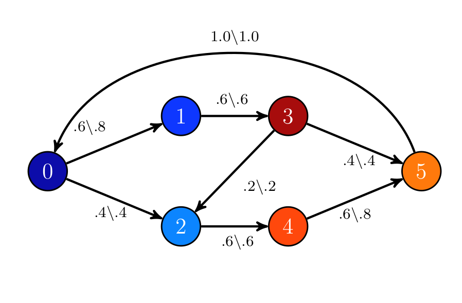
(a) Circulation $\mathcal{I}$. Each edge $(i,j)$ in the figure is labeled as $\mathcal{I}_{i,j}\setminus c(i,j)$.

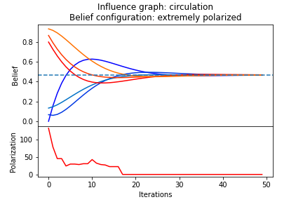
(b) Evolution of belief and polarization under an extreme polarized initial belief configuration

Figure 4: Evolution of beliefs and polarization in a circulation graph

An invariant property of balanced influence is that the overall sum of beliefs remains the same across time.

Lemma 5

If the influence graph $\mathcal{I}$ is balanced then $\sum_{i\in\mathcal{A}}B^{t}_{i}=\sum_{i\in\mathcal{A}}B^{t+1}_{i}$.

Proof

By Def.2 we have $\sum_{i\in\mathcal{A}}B^{t+1}_{i}=\sum_{i\in\mathcal{A}}\left(B^{t}_{i}+\nicefrac{{1}}{{|\mathcal{A}|}}\sum_{j\in\mathcal{A}}\mathcal{I}_{j,i}(B^{t}_{j}-B^{t}_{i})\right)$ hence $\sum_{i\in\mathcal{A}}B^{t+1}_{i}=\sum_{i\in\mathcal{A}}B^{t}_{i}+\nicefrac{{1}}{{|\mathcal{A}|}}\left(\sum_{i\in\mathcal{A}}\sum_{j\in\mathcal{A}}\mathcal{I}_{j,i}B^{t}_{j}-\sum_{i\in\mathcal{A}}\sum_{j\in\mathcal{A}}\mathcal{I}_{j,i}B^{t}_{i}\right).$ Using the fact that $\sum_{i\in\mathcal{A}}\sum_{j\in\mathcal{A}}\mathcal{I}_{j,i}B^{t}_{j}=\sum_{i\in\mathcal{A}}\sum_{j\in\mathcal{A}}\mathcal{I}_{i,j}B^{t}_{i}$ and Def. 9 we obtain $\sum_{i\in\mathcal{A}}B^{t+1}_{i}=\sum_{i\in\mathcal{A}}B^{t}_{i}+\nicefrac{{1}}{{|\mathcal{A}|}}\sum_{i\in\mathcal{A}}\sum_{j\in\mathcal{A}}B^{t}_{i}(\mathcal{I}_{j,i}-\mathcal{I}_{i,j})=\sum_{i\in\mathcal{A}}B^{t}_{i}.$

We shall use a fundamental property from flow networks describing flow conservation for graph cuts [8]. Interpreted in our case it tells us that any group of agents $A\subseteq\mathcal{A}$ influences other groups as much as they influence $A$.

Proposition 7 (Group Influence Conservation)

Suppose that $\mathcal{I}$ is balanced. Let $\{A,B\}$ be a partition of $\mathcal{A}$. Then $\sum_{i\in A}\sum_{j\in B}\mathcal{I}_{i,j}=\sum_{i\in A}\sum_{j\in B}\mathcal{I}_{j,i}$.

Proof

Immediate consequence of Prop. 6.1.1 in [8].

We now define weakly connected influence. Recall that an undirected graph is connected if there is path between each pair of nodes.

Definition 10 (Weakly Connected Influence)

Given an influence graph $\mathcal{I}$ define the undirected graph $G_{\mathcal{I}}=(\mathcal{A},E)$ where $\{i,j\}\in E$ if and only if $\mathcal{I}_{i,j}>0$ or $\mathcal{I}_{j,i}>0$. An influence graph $\mathcal{I}$ is called weakly connected if the undirected graph $G_{\mathcal{I}}$ is connected.

Weakly connected influence is a significant relaxation of its strongly connected counterpart. Nevertheless we shall show next that every weakly connected influence that is balanced it also strongly connected. The flow network intuition behind this property is that a circulation flow never leaves strongly connected components.

Lemma 6

If $\mathcal{I}$ is balanced and $\mathcal{I}_{i,j}>0$ then $j\stackrel{{\scriptstyle\,\,\,\,}}{{\leadsto}}i$.

Proof

For the sake of contradiction, assume that $\mathcal{I}$ is balanced (a circulation) and $\mathcal{I}_{i,j}>0$ but there is no path from $j$ to $i$. Define the agents reachable from $j$, $R_{j}=\{k\in\mathcal{A}|\ j\stackrel{{\scriptstyle\,\,\,\,}}{{\leadsto}}k\}\cup\{j\}$ and let $\overline{R}_{j}=\mathcal{A}\setminus R_{j}$. Notice that $(R_{j},\overline{R}_{j})$ is a partition of $\mathcal{A}.$ Since the codomain of $\mathcal{I}$ is $[0,1]$, $i\in\overline{R}_{j}$, $j\in R_{j}$ and $\mathcal{I}_{i,j}>0$ we obtain $\sum_{k\in R_{j}}\sum_{l\in\overline{R}_{j}}\mathcal{I}_{l,k}>0$. Clearly there is no $k\in R_{j},l\in\overline{R}_{j}$ such that $\mathcal{I}_{k,l}>0$, therefore $\sum_{k\in R_{j}}\sum_{l\in\overline{R}_{j}}\mathcal{I}_{k,l}=0$ which contradicts Prop.7. ∎

Theorem 5.4 (Weakly-Connected Balanced Influence)

If the influence graph $\mathcal{I}$ is balanced and weakly connected then $\mathcal{I}$ is also strongly connected.

Proof

Immediate consequence of Lem.6 and Def. 10.

It then follows that in a scenario in which every agent influences every other agent directly or indirectly and they influence as much as they are influenced, their beliefs converge to the average of initial beliefs.

Theorem 5.5 (Consensus Value)

If the influence graph $\mathcal{I}$ is balanced and weakly connected then $\lim_{t\to\infty}B^{t}_{i}=\nicefrac{{1}}{{|\mathcal{A}|}}\sum_{j\in\mathcal{A}}B^{0}_{j}.$

Proof

It is an immediate consequence of Th.5.4, Lem. 5 and Th. 5.3.

We conclude this section on balanced influence by highlighting the importance of Th.5.4. Recall that $\mathcal{I}$ being strongly connected implies belief converge to the same value (Th. 5.3) which in turn implies that polarization disappears (i.e., it converges to zero). Then Th.5.4 tells us that if polarization does not disappear then either $\mathcal{I}$ is not weakly connected or $\mathcal{I}$ is not balanced. If $\mathcal{I}$ is not weakly connected then there must be isolated subgroups of agents. E.g., consider a scenario with two isolated strongly-connected components; the members of the same component will achieve consensus but the consensus values of the two components may be very different. This is illustrated in the fourth row of Fig. 3, representing the simulations for a disconnected influence graph (schematically depicted in Fig. 2(c)). Now if $\mathcal{I}$ is not balanced then there there must be at least one agent that influences more than what he is influenced (or vice versa). E.g., consider the fifth row of Fig. 3, representing the simulations for a pair of unrelenting influencers (schematically depicted in Fig. 2(d)) with high influence over other agents but little or no influence from other agents over themselves.

6 Confirmation Bias

The previous sections show that the update function of Def. 2, although simple, can shed light on important aspects of polarization. As a step further, here we consider a refinement of the model that can capture bias not only towards agents, but towards opinions themselves. This bias, known in social psychology as confirmation bias [3], is manifest when an agent tends to give more weight to evidence supporting their current beliefs than to evidence contradicting them, independently from its source.

We can incorporate confirmation bias into our model as follows. When agent $j$ presents agent $i$ with evidence for or against proposition $p$, the update function will still move agent $i$’s belief toward the belief of agent $j$, proportionally to the influence $\mathcal{I}_{j,i}$ that $j$ has over $i$, but with a caveat: the move is stronger when $j$’s belief is similar to $i$’s than when it is dissimilar. This is formalized as follows.

Definition 11 (Confirmation-bias update-function)

The confirmation-bias update-function $\mu^{\textit{CB}}{:}B{\times}\mathcal{I}{\rightarrow}B$ is defined analogously to the update function of Definition 2, with the sole difference that the effect of agent $j$ on agent $i$’s belief at time $t{+}1$, once both agents interact at time $t$, is given by $B^{t}_{i{\mid}j}{=}B^{t}_{i}{+}f^{t}_{i,j}\,\mathcal{I}_{j,i}\,(B^{t}_{j}{-}B^{t}_{i})$, where $f^{t}_{i,j}{\in}[0,1]$ is a confirmation-bias factor proportional to the difference in the agents beliefs, defined as $f^{t}_{i,j}{=}1{-}|B^{t}_{j}{-}B^{t}_{i}|$.

The incorporation of confirmation bias into our model allows for the uncovering of new, interesting phenomena. Fig. 5 illustrates the evolution of polarization, starting from a tripolar belief configuration, in a faintly communicating influence graph (schematically depicted in Fig. 5(a)) representing a social network divided into two groups that evolve mostly separately, with little communication between them. If agents employ the original update (Fig.5(b)), they are quickly influenced towards a midpoint between their beliefs, reaching consensus and eliminating polarization. On the other hand, if agents employ confirmation-bias update (Fig.5(c)), convergence happens significantly more slowly, extending polarization further in time. Note that, in this case, confirmation bias emphasizes the non-monotonicity of polarization: since each group reaches an internal consensus relatively quickly, polarization increases; but as each group slowly communicates, general consensus is eventually achieved.

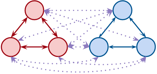
(a) Scheme of faintly communicating influence

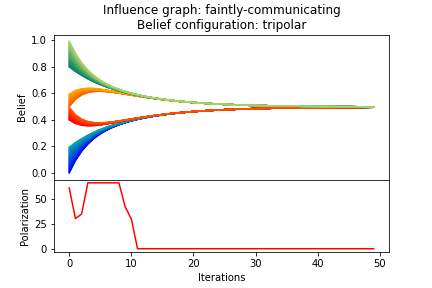
(b) Original update function

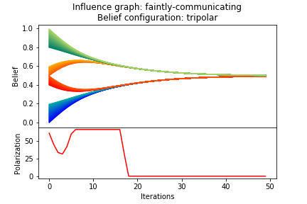
(c) Confirmation-bias update function with constant factor $f^{t}_{i,j}{=}0.5$

Figure 5: Evolution of polarization for tripolar initial belief configuration and faintly-communication influence, with $n{=}100$ agents

Note that the confirmation-bias update function generalizes Def.2, since the latter is the special case of the former in which the confirmation-bias factor is always 1. The proof of Th.5.3 can be easily modified (see Appendix 0.A) to show that, also under confirmation bias, in strongly connected influence graphs all agents’ beliefs eventually converge to the same value (with the sole exception of a society in which all agents possess extreme beliefs of 0 or 1). This implies that polarization vanishes over time, even if at a slower pace, in the absence of external influences. This is formalized below.

Theorem 6.1 (Partial belief consensus under confirmation bias)

In a strongly connected influence graph and under the confirmation-bias update-function, if there exists an agent $k\in\mathcal{A}$ such that $B^{0}_{k}\notin\{0,1\}$ then for every $i,j\in\mathcal{A}$, $\lim_{t\to\infty}B^{t}_{i}=\lim_{t\to\infty}B^{t}_{j}$. Otherwise for every $i\in\mathcal{A}$, $B^{t}_{i}=B^{t+1}_{i}\in\{0,1\}$.

7 Conclusions

We considered a model for polarization and belief evolution for multi-agents systems. We showed that in strongly-connected influence graphs, agents always reach consensus, so polarization goes to $0$ regardless of initial beliefs or whether agents have confirmation-bias. In the absence of confirmation bias, for balanced families we provided the actual consensus value, and for cliques also the time after which a given opinion difference $\epsilon>0$ is reached. We showed that if polarization does not disappear then either there is an isolated group of agents or there is an agent that influences more than what he is in influenced (Th.5.4). We showed weakly-connected influence graphs where polarization does not converge to zero and several simulations illustrating polarization in the model. We believe that our formal results bring some insights about the phenomenon of polarization, which may help in the design of more robust computational models for human cognitive and social processes.

As future work we will study belief updates based on the backfire effect, which is manifest when, in the face of contradictory evidence, agents’ beliefs are not corrected, but rather remain unaltered or even get stronger. The effect has been demonstrated in experiments by psychologists and sociologists [20, 9, 14].

Appendix 0.A Proofs

0.A.1 Strongly Connected Influence (Confirmation Bias)

Remark 1

All proofs in this section use the confirmation-bias update-function from Def. 11, thus note that, although sometimes Theorems look the same as the ones in Section 4, their claims differ in the update-function used, which sometimes we will not highlight for the sake of brevity. Also assume, from now on, that there are no two agents $i,j\in\mathcal{A}$ such that $B^{0}_{i}=0$ and $B^{0}_{j}=1$ thus for every $i,j\in\mathcal{A}$: $f^{0}_{i,j}>0$. This might look like a bold assumption but in the end of this section we will address the cases in which this condition does not hold.

We need to following equation which can be obtained directly from Def.11.

$$B^{t{+}1}_{i}=B^{t}_{i}+\frac{1}{|\mathcal{A}|}\sum_{j\in\mathcal{A}}f^{t}_{i,j}\mathcal{I}_{j,i}(B^{t}_{j}-B^{t}_{i})=B^{t}_{i}+\frac{1}{|\mathcal{A}|}\sum_{j\in\mathcal{A}\setminus\{i\}}f^{t}_{i,j}\mathcal{I}_{j,i}(B^{t}_{j}-B^{t}_{i})$$ (3)

The following lemma states a distinctive property of strongly connected influence: The belief value of any agent at any time is bounded by those from extreme agents in the previous time unit.

Lemma 7 (Belief Bounds)

Assume that the influence graph $\mathcal{I}$ is strongly connected. Then for every $i\in\mathcal{A}$, $min^{t}\leq B^{t{+}1}_{i}\leq max^{t}.$

Proof

We want to prove $B^{t{+}1}_{i}\leq max^{t}$. Since $B^{t}_{j}\leq max^{t}$, we can use Eq.2 to derive the inequality $B^{t{+}1}_{i}\leq E_{1}\stackrel{{\scriptstyle\textup{{def}}}}{{=}}B^{t}_{i}+\frac{1}{|\mathcal{A}|}\sum_{j\in\mathcal{A}}f^{t}_{i,j}\mathcal{I}_{j,i}(max^{t}-B^{t}_{i}).$ Furthermore, $E_{1}\leq E_{2}\stackrel{{\scriptstyle\textup{{def}}}}{{=}}B^{t}_{i}+\frac{1}{|\mathcal{A}|}\sum_{j\in\mathcal{A}}(max^{t}-B^{t}_{i})$ because $f^{t}_{i,j}\mathcal{I}_{j,i}\leq 1$ and $max^{t}-B^{t}_{i}\geq 0.$ We thus obtain $B^{t{+}1}_{i}\leq E_{2}=B^{t}_{i}+\frac{|\mathcal{A}|}{|\mathcal{A}|}(max^{t}-B^{t}_{i})=B^{t}_{i}+max^{t}-B^{t}_{i}=max^{t}$ as wanted. The proof of $min^{t}\leq B^{t{+}1}_{i}$ is similar. ∎

Corollary 4

For all times $t$, there are no agents $i,j\in\mathcal{A}$ such that $B^{t}_{i}=0$ and $B^{t}_{j}=1$, thus for every $i,j\in\mathcal{A}$: $f^{t}_{i,j}>0$.

Proof

It is an immediate consequence of the assumption we made that $i,j\in\mathcal{A}$ such that $B^{0}_{i}=0$ and $B^{0}_{j}=1$ and Lemma 7

An immediate consequence of the above lemma, the next corollary tells us that $min^{\cdot}$ and $max^{\cdot}$ are monotonically increasing and decreasing functions.

Corollary 5 (Monotonicity of Extreme Beliefs)

If the influence graph $\mathcal{I}$ is strongly connected then $max^{t+1}\leq max^{t}$ and $min^{t+1}\geq min^{t}$ for all $t\in\mathbb{N}$.

The above monotonicity property and the fact that both $max^{\cdot}$ and $min^{\cdot}$ are bounded between $0$ and $1$ lead us, via the monotonic convergence theorem [8], to the existence of limits for the beliefs of extreme agents.

Corollary 6 (Limits of Extreme Beliefs)

If the influence graph $\mathcal{I}$ is strongly connected then $\underset{t\to\infty}{\lim}max^{t}=U$ and $\underset{t\to\infty}{\lim}min^{t}=L$ for some $U$, $L\in[0,1]$.

Another distinctive property of agents under strongly component influence is that the belief of any agent at time $t$ will influence every other agent by the time $t+|\mathcal{A}|-1$. The precise statement of this property is given below in the Path Influence Lemma (Lem.8). First we need the following rather technical proposition to prove the lemma.

Proposition 8

Assume $\mathcal{I}$ is strongly connected. Let $i,k\in\mathcal{A}$, $n,t\in\mathbb{N}$ with $n\geq 1$, and $v\in[0,1].$

1. If $B^{t}_{i}\leq v$ then $B^{t{+}1}_{i}\leq v+\frac{1}{|\mathcal{A}|}\sum_{j\in\mathcal{A}}f^{t}_{i,j}\mathcal{I}_{j,i}\left(B^{t}_{j}-v\right).$

2. $B^{t+n}_{i}\leq max^{t}+\frac{1}{|\mathcal{A}|}f^{t+n-1}_{i,k}\mathcal{I}_{k,i}(B^{t+n-1}_{k}-max^{t}).$

Proof

Let $i,k\in\mathcal{A}$, $n,t\in\mathbb{N}$ with $n\geq 1$, and $v\in[0,1].$

1. From Def.11 we obtain $B^{t{+}1}_{i}=\frac{1}{|\mathcal{A}|}\sum_{j\in\mathcal{A}}\left(B^{t}_{i}(1-f^{t}_{i,j}\mathcal{I}_{j,i})+f^{t}_{i,j}\mathcal{I}_{j,i}B^{t}_{j}\right)$. If $B^{t}_{i}\allowbreak\leq v$ then $B^{t{+}1}_{i}\leq\frac{1}{|\mathcal{A}|}\sum_{j\in\mathcal{A}}\big{(}v(1-f^{t}_{i,j}\mathcal{I}_{j,i})+f^{t}_{i,j}\mathcal{I}_{j,i}B^{t}_{j}\big{)}$ which is equal to $v+\frac{1}{|\mathcal{A}|}\sum_{j\in\mathcal{A}}f^{t}_{i,j}\mathcal{I}_{j,i}\big{(}B^{t}_{j}-v\big{)}$.

2. By Def.11 $B^{t+n}_{i}=\frac{1}{|\mathcal{A}|}\sum_{j\in\mathcal{A}}\big{(}B^{t+n-1}_{i}+f^{t+n-1}_{i,j}\mathcal{I}_{j,i}(B^{t+n-1}_{j}-B^{t+n-1}_{i})\big{)}.$ From Cor.5 we have $B^{t+n}_{i}\leq max^{t+n}\leq max^{t+n-1}$. Thus by Prop.8(1):

   $$B^{t+n}_{i} \leq\frac{1}{|\mathcal{A}|}\sum_{j\in\mathcal{A}}\left(max^{t+n-1}+f^{t+n-1}_{i,j}\mathcal{I}_{j,i}(B^{t{+}n{-}1}_{j}-max^{t+n-1})\right)$$

   $$=max^{t+n-1}+\frac{1}{|\mathcal{A}|}\sum_{j\in\mathcal{A}}f^{t+n-1}_{i,j}\mathcal{I}_{j,i}(B^{t+n-1}_{j}-max^{t+n-1})$$

   Let us define the sum $S=\sum_{j\in\mathcal{A}\setminus\{k\}}f^{t+n-1}_{i,j}\mathcal{I}_{j,i}(B^{t{+}n{-}1}_{j}-max^{t+n-1})$ and the fraction $F=\frac{1}{|\mathcal{A}|}f^{t+n-1}_{i,k}\mathcal{I}_{k,i}(B^{t{+}n{-}1}_{k}-max^{t+n-1}).$ Therefore, $B^{t{+}n}_{i}\leq max^{t+n-1}+\frac{1}{|\mathcal{A}|}S+F.$ Since $max^{t+n-1}\geq B^{t{+}n{-}1}_{j}$ for each $j\in\mathcal{A}$ then $S\leq 0$. We thus obtain $B^{t{+}n}_{i}\leq max^{t+n-1}+F=max^{t+n-1}(1-\frac{1}{|\mathcal{A}|}f^{t+n-1}_{i,k}\mathcal{I}_{k,i})+\frac{1}{|\mathcal{A}|}f^{t+n-1}_{i,k}\mathcal{I}_{k,i}B^{t{+}n{-}1}_{k}.$ Notice that $\frac{1}{|\mathcal{A}|}f^{t+n-1}_{i,k}\mathcal{I}_{k,i}$ is in $[0,1]$ and from Cor.1, $\allowbreak max^{t+n-1}\leq max^{t}$. We can then conclude $B^{t{+}n}_{i}\leq max^{t}+\frac{1}{|\mathcal{A}|}f^{t+n-1}_{i,k}\mathcal{I}_{k,i}\allowbreak\big{(}B^{t{+}n{-}1}_{k}-max^{t}\big{)}$ as wanted.

∎

Definition 12 (Min Confirmation-bias)

Denote by $f_{min}=\min_{i,j\in\mathcal{A}}f^{0}_{i,j}$ the minimum confirmation-bias factor in our graph throughout time. fancyline]Frank: The explanation shouldn’t be part of the definition: ”Since $min^{t}$ and $max^{t}$ … I moved it outside

Notice that since $min^{t}$ and $max^{t}$ get closer as $t$ (Cor.5), $f_{min}$ does not decrease when time passes, thus, it acts as a lower bound for the confirmation-bias factor in every time step.

The following property intuitively tells us that an agent $i$ at time $t$ will bound the belief of $j$ at time $t+t^{\prime}$ where $t^{\prime}$ is the size of any influence path from $i$ and $j$. The bound depends on the belief of agent $i$ at time $t$ and the product influence $C$ of $i$ over $j$ along the corresponding path.

Lemma 8 (Path Influence)

Assume that $\mathcal{I}$ is strongly connected. Let $p$ be an arbitrary path $i\stackrel{{\scriptstyle\,\,C\,\,}}{{\leadsto_{p}}}j$. Then $B^{t+|p|}_{j}\leq max^{t}+\frac{Cf_{min}^{|p|}}{|\mathcal{A}|^{|p|}}(B^{t}_{i}-max^{t}).$

Proof

Let $p$ be the path $i_{0}\stackrel{{\scriptstyle\,\,\small\tiny{C_{1}}\,\,}}{{\rightarrow}}i_{1}\stackrel{{\scriptstyle\,\,\small\tiny{C_{2}}\,\,}}{{\rightarrow}}\ldots\stackrel{{\scriptstyle\,\,\small\tiny{C_{n}}\,\,}}{{\rightarrow}}i_{n}.$ We show that $B^{t+|p|}_{i_{n}}\leq max^{t}+\frac{Cf_{min}}{|\mathcal{A}|}(B^{t}_{i_{0}}-max^{t})$ where $C=C_{1}\times\ldots\times C_{n}.$ We proceed by induction on $n$. For $n=1$, since $B^{t}_{i_{0}}-max^{t}\leq 0$ we obtain the result immediately from Prop.8(2). Assume that $B^{t+|p^{\prime}|}_{i_{n-1}}\leq max^{t}+\frac{C^{\prime}f_{min}^{|p^{\prime}|}}{|\mathcal{A}|^{|p^{\prime}|}}(B^{t}_{i_{0}}-max^{t})$ where $p^{\prime}=i_{0}\stackrel{{\scriptstyle\,\,\small\tiny{C_{1}}\,\,}}{{\rightarrow}}i_{1}\stackrel{{\scriptstyle\,\,\small\tiny{C_{2}}\,\,}}{{\rightarrow}}\ldots\stackrel{{\scriptstyle\,\,\small\tiny{C_{n-1}}\,\,}}{{\rightarrow}}i_{n-1}$ and $C^{\prime}=C_{1}\times\ldots\times C_{n-1}$ with $n>1$. Notice that $|p^{\prime}|=|p|-1$. Using Prop.8(2) and the fact that $B^{t+|p^{\prime}|}_{i_{n-1}}-max^{t}\leq 0$ we obtain $B^{t+|p|}_{i_{n}}\leq max^{t}+\frac{C_{n}f_{min}}{|\mathcal{A}|}(B^{t+|p^{\prime}|}_{i_{n-1}}-max^{t}).$ Using our assumption we obtain $B^{t+|p|}_{i_{n}}\leq max^{t}+\frac{C_{n}f_{min}}{|\mathcal{A}|}(max^{t}+\frac{C^{\prime}f_{min}^{|p^{\prime}|}}{|\mathcal{A}|^{|p^{\prime}|}}(B^{t}_{i_{0}}-max^{t})-max^{t})=max^{t}+\frac{Cf_{min}^{|p|}}{|\mathcal{A}|^{|p|}}(B^{t}_{i_{0}}-max^{t})$ as wanted.

Theorem 0.A.1

Assume that $\mathcal{I}$ is strongly connected. Let $\mathtt{m}^{t}\in\mathcal{A}$ be a minimal agent at time $t$ and $p$ be a path such that $\mathtt{m}^{t}\stackrel{{\scriptstyle\,\,\,\,}}{{\leadsto_{p}}}i$. Then

$B^{t{+}|p|}_{i}\leq max^{t}-\delta^{t}$, with $\delta^{t}=\left(\frac{\mathcal{I}_{min}f_{min}}{|\mathcal{A}|}\right)^{|p|}(U-L)$.

Proof

Suppose that $p$ is the path $\mathtt{m}^{t}\stackrel{{\scriptstyle\,\,C\,\,}}{{\leadsto_{p}}}i$. From Lem.8 we obtain $B^{t+|p|}_{i}\leq max^{t}+\frac{Cf_{min}^{|p|}}{|\mathcal{A}|^{|p|}}(B^{t}_{\mathtt{m}^{t}}-max^{t})=max^{t}+\frac{Cf_{min}^{|p|}}{|\mathcal{A}|^{|p|}}(min^{t}-max^{t}).$ Since $\frac{Cf_{min}^{|p|}}{|\mathcal{A}|^{|p|}}(min^{t}-max^{t})\leq 0$, we can substitute $C$ with $\mathcal{I}_{min}^{|p|}$. Thus, $B^{t+|p|}_{i}\leq max^{t}+\Big{(}\frac{\mathcal{I}_{min}f_{min}}{|\mathcal{A}|}\Big{)}^{|p|}\allowbreak(min^{t}-max^{t}).$ From Cor.6, the maximum value of $min^{t}$ is $L$ and the minimum value of $max^{t}$ is $U$, thus $B^{t+|p|}_{i}\leq max^{t}+\Big{(}\frac{\mathcal{I}_{min}f_{min}}{|\mathcal{A}|}\Big{)}^{|p|}(L-U)=max^{t}-\delta^{t}.$

Proposition 9

Suppose that $\mathcal{I}$ is strongly connected. If $B^{t{+}n}_{i}\leq max^{t}-\gamma$ and $\gamma\geq 0$ then $B^{t+n+1}_{i}\leq max^{t}-\frac{\gamma}{|\mathcal{A}|}.$

Proof

Using Prop.8(1) followed by the assumption $B^{t{+}n}_{i}\leq max^{t}-\gamma$ for $\gamma\geq 0$ and the fact that $\mathcal{I}_{j,i}\in[0,1]$ we obtain the inequality $B^{t+n+1}_{i}\leq max^{t}-\gamma+\frac{1}{|\mathcal{A}|}\sum_{j\in\mathcal{A}\setminus\{i\}}f^{t+n}_{i,j}\mathcal{I}_{j,i}\left(B^{t{+}n}_{j}-(max^{t}-\gamma)\right).$ From Cor.1 $max^{t}\geq max^{t+n}\geq B^{t+n}_{j}$ for every $j\in\mathcal{A}$, hence $B^{t+n+1}_{i}\leq max^{t}-\gamma+\frac{1}{|\mathcal{A}|}\sum_{j\in\mathcal{A}\setminus\{i\}}f^{t+n}_{i,j}\mathcal{I}_{j,i}\big{(}max^{t}-(max^{t}-\gamma)\big{)}.$ Since $f^{t+n}_{i,j}\mathcal{I}_{j,i}\in[0,1]$ we derive $B^{t+n+1}_{i}\leq max^{t}-\gamma+\frac{1}{|\mathcal{A}|}\sum_{j\in\mathcal{A}\setminus\{i\}}\gamma\allowbreak=max^{t}-\frac{\gamma}{|\mathcal{A}|}.$ ∎

Theorem 0.A.2

If $\mathcal{I}$ is strongly connected then $B^{t+|\mathcal{A}|-1}_{i}\leq max^{t}-\epsilon$, where $\epsilon$ is equal to $\left(\frac{\mathcal{I}_{min}f_{min}}{|\mathcal{A}|}\right)^{|\mathcal{A}|-1}(U-L)$.

Proof

Let $p$ be the path $\mathtt{m}^{t}\stackrel{{\scriptstyle\,\,\,\,}}{{\leadsto_{p}}}i$ where $\mathtt{m}^{t}\in\mathcal{A}$ is minimal agent at time $t$ and let $\delta^{t}=\left(\frac{\mathcal{I}_{min}f_{min}}{|\mathcal{A}|}\right)^{|p|}(U-L)$. If $|p|=|\mathcal{A}|-1$ then the result follows from Th.0.A.1. Else $|p|<|\mathcal{A}|-1$ by Def.5. We first show by induction on $m$ that $B^{t+|p|+m}_{i}\leq max^{t}-\frac{\delta^{t}}{|\mathcal{A}|^{m}}$ for every $m\geq 0$. If $m=0$, $B^{t+|p|}_{i}\leq max^{t}-\delta^{t}$ by Th.0.A.1. If $m>0$ and $B^{t+|p|+(m-1)}_{i}\leq max^{t}-\frac{\delta^{t}}{|\mathcal{A}|^{m-1}}$ then $B^{t+|p|+m}_{i}\leq max^{t}-\frac{\delta^{t}}{|\mathcal{A}|^{m}}$ by Prop.9. Therefore, take $m=|\mathcal{A}|-|p|-1$ to obtain $B^{t+|\mathcal{A}|-1}_{i}\leq max^{t}-\frac{\delta^{t}}{|\mathcal{A}|^{|\mathcal{A}|-|p|-1}}=max^{t}-\frac{(\mathcal{I}_{min}f_{min})^{|p|}.(U-L)}{|\mathcal{A}|^{|\mathcal{A}|-1}}\leq max^{t}-\epsilon$ as wanted. ∎

Corollary 7

$max^{t+m(|\mathcal{A}|-1)}\leq max^{t}-m\epsilon$ for $\epsilon$ as in Th.0.A.2.

Theorem 0.A.3

If $\mathcal{I}$ is strongly connected then $\lim_{t\to\infty}max^{t}=\lim_{t\to\infty}min^{t}.$

Proof

Suppose, by contradiction, that $\lim_{t\to\infty}max^{t}=U\neq L=\lim_{t\to\infty}min^{t}$. Let $\epsilon=\left(\frac{\mathcal{I}_{min}f_{min}}{|\mathcal{A}|}\right)^{|\mathcal{A}|-1}(U-L).$ From the assumption $U>L$ therefore $\epsilon>0$. Take $t=0$ and $m=\left(\lceil\frac{1}{\epsilon}\rceil+1\right)$. Using Cor.3 we obtain $max^{0}\geq max^{{m(|\mathcal{A}|-1)}}+m\epsilon.$ Since $m\epsilon>1$ and $max^{m(|\mathcal{A}|-1)}\geq 0$ then $max^{0}>1.$ But this contradicts Def.7 which states that $max^{0}\in[0,1]$.∎

As an immediate consequence of Th.5.2 and the squeeze theorem, we conclude that for strongly-connected graphs, the belief of all agents converge to the same value.

Theorem 0.A.4

If $\mathcal{I}$ is strongly connected then for each $i,j\in\mathcal{A},\underset{t\to\infty}{\lim}B^{t}_{i}=\underset{t\to\infty}{\lim}B^{t}_{j}.$

We assumed, in the beginning of this section, that there were no two agents $i,j$ such that $B^{t}_{i}=0$ and $B^{t}_{j}=1$, now we will address the situation in which this does not happen, thus, assuming that those agents $i$ and $j$ existed, we are left with two cases. Before showing them, we must prove a technical proposition.

Proposition 10 (Influencing the extremes)

Supposing that $\mathcal{I}$ is strongly connected and that there exists an agent $k$ such that $B^{0}_{k}\notin\{0,1\}$, $max^{|\mathcal{A}-1|}<1$.

Proof

It is enough to show that, for every $i$, being $p$ a path $k\stackrel{{\scriptstyle\,\,\,\,}}{{\leadsto_{p}}}i$, $B^{|p|}_{i}<1$ such that $p=ki_{1}i_{2}\ldots i_{n-1}i_{n}..i$. We will prove it by induction in $n=|k\stackrel{{\scriptstyle\,\,\,\,}}{{\leadsto_{p}}}i_{n}|$. For $n=0$, it is true via the hypothesis. For $n>1$, we have, by the inductive hypothesis and Def. 5, that $B^{|p|-1}_{i_{n-1}}<1$ and $\mathcal{I}_{i_{n-1},n}>0$. Thus, $B^{|p|}_{i_{n}}=B^{|p|-1}_{i_{n}}+\frac{1}{|\mathcal{A}|}\sum_{j\in\mathcal{A}}f^{|p|-1}_{i_{n},j}\mathcal{I}_{j,i_{n}}(B^{|p|-1}_{j}-B^{|p|-1}_{i_{n}})$ separating $i_{n-1}$ from the summation we get that it $B^{|p|}_{i_{n}}=B^{|p|-1}_{i_{n}}+\frac{1}{|\mathcal{A}|}\sum_{j\in\mathcal{A}\setminus{}\{i_{n-1}\}}f^{|p|-1}_{i_{n},j}\mathcal{I}_{j,i_{n}}(B^{|p|-1}_{j}-B^{|p|-1}_{i_{n}})+\frac{1}{|\mathcal{A}|}f^{|p|-1}_{i_{n},i_{n-1}}\allowbreak\mathcal{I}_{i_{n-1},i_{n}}(B^{|p|-1}_{i_{n-1}}-B^{|p|-1}_{i_{n}})\allowbreak\leq 1+\frac{1}{|\mathcal{A}|}f^{|p|-1}_{i_{n},i_{n-1}}\mathcal{I}_{i_{n-1},i_{n}}(B^{|p|-1}_{i_{n-1}}-1)<1$. ∎

The following Theorem is the confirmation-bias version of Thr. 5.3 and tells us that beliefs always converge and that, unless the society is composed only by very extreme agents, they converge to the same value.

Theorem 0.A.5 (Confirmation-bias belief convergence)

In a strongly connected influence graph and under the confirmation-bias update-function, if there exists an agent $k\in\mathcal{A}$ such that $B^{0}_{k}\notin\{0,1\}$ then for every $i,j\in\mathcal{A}$, $\lim_{t\to\infty}B^{t}_{i}=\lim_{t\to\infty}B^{t}_{j}$. Otherwise for every $i\in\mathcal{A}$, $B^{t}_{i}=B^{t+1}_{i}\in\{0,1\}$.

Proof

1. If there exists an agent $k\in\mathcal{A}$ such that $B^{0}_{k}\notin\{0,1\}$, we can use Prop. 10 to show that by the time $|\mathcal{A}|-1$ no agent has belief $1$, thus we fall on the general case stated in the beginning of the section (starting at a different time step does not make any difference for this purposes) and, thus, all beliefs converge to the same value according to Thr. 0.A.4.

2. Otherwise it is easy to see that beliefs remain constant as $0$ or $1$ throughout time, since the agents are so biased towards each other the only agents $j$ able to influence another agent $i$ ($f^{t}_{i,j}\neq 0$) have the same belief as $i$.

∎

Appendix 0.B Axioms for Esteban-Ray polarization measure

The Esteban-Ray polarization measure used in this paper was developed as the only function satisfying all of the following conditions and axioms [11]:

Condition H:

The ranking induced by the polarization measure over two distributions is invariant w.r.t. the size of the population. (This is why we can assume w.l.o.g. that the distribution is a probability distribution.)

$$\rho_{\mathit{ER}}(\pi,y)\geq\rho_{\mathit{ER}}(\pi^{\prime},y^{\prime})\implies\forall\lambda>0,\rho_{\mathit{ER}}(\lambda\pi,y)\geq\rho_{\mathit{ER}}(\lambda\pi^{\prime},y^{\prime})~{}.$$

Axiom 1:

Consider three levels of belief $p,q,r\in[0,1]$ such that the same proportion of the population holds beliefs $q$ and $r$, and a significantly higher proportion of the population holds belief $p$. If the groups of agents that hold beliefs $q$ and $r$ reach a consensus and agree on an “average” belief $\nicefrac{{(q+r)}}{{2}}$, then the social network becomes more polarized.

Axiom 2:

Consider three levels of belief $p,q,r\in[0,1]$, such that $q$ is at least as close to $r$ as it is to $p$, and $p>r$. If only small variations on $q$ are permitted, the direction that brings it closer to the nearer and smaller opinion ($r$) should increase polarization.

Axiom 3:

Consider three levels of belief $p,q,r\in[0,1]$, s.t. $p<q<r$ and there is a non-zero proportion of the population holding belief $q$. If the proportion of the population that holds belief $q$ is equally split into holding beliefs $q$ and $r$, then polarization increases.

References

- [1] Alvim, M.S., Amorim, B., Knight, S., Quintero, S., Valencia, F.: (2020), https://github.com/Sirquini/Polarization
- [2] Alvim, M.S., Knight, S., Valencia, F.: Toward a formal model for group polarization in social networks. In: The Art of Modelling Computational Systems. Lecture Notes in Computer Science, vol. 11760, pp. 419–441. Springer (2019)
- [3] Aronson, E., Wilson, T., Akert, R.: Social Psychology. Upper Saddle River, NJ : Prentice Hall, 7 edn. (2010)
- [4] Bozdag, E.: Bias in algorithmic filtering and personalization. Ethics and Information Technology (09 2013). https://doi.org/10.1007/s10676-013-9321-6
- [5] Calais Guerra, P., Meira Jr, W., Cardie, C., Kleinberg, R.: A measure of polarization on social media networks based on community boundaries. Proceedings of the 7th International Conference on Weblogs and Social Media, ICWSM 2013 pp. 215–224 (01 2013)
- [6] Christoff, Z., et al.: Dynamic logics of networks: information flow and the spread of opinion. Ph.D. thesis, PhD Thesis, Institute for Logic, Language and Computation, University of … (2016)
- [7] DeGroot, M.H.: Reaching a consensus. Journal of the American Statistical Association 69(345), 118–121 (1974), http://www.jstor.org/stable/2285509
- [8] Diestel, R.: Graph Theory. Springer-Verlag, fifth ed edn. (2015)
- [9] Ditto, P.H., Lopez, D.F.: Motivated skepticism: Use of differential decision criteria for preferred and nonpreferred conclusions. Journal of Personality and Social Psychology 63(4), 568 (1992)
- [10] Elder, A.: The interpersonal is political: unfriending to promote civic discourse on social media. Ethics and Information Technology pp. 1–10 (2019)
- [11] Esteban, J.M., Ray, D.: On the measurement of polarization. Econometrica 62(4), 819–851 (1994), http://www.jstor.org/stable/2951734
- [12] Gargiulo, F., Gandica, Y.: The role of homophily in the emergence of opinion controversies. arXiv preprint arXiv:1612.05483 (2016)
- [13] Golub, B., Jackson, M.O.: Naïve learning in social networks and the wisdom of crowds. American Economic Journal: Microeconomics 2(1), 112–49 (February 2010). https://doi.org/10.1257/mic.2.1.112, https://www.aeaweb.org/articles?id=10.1257/mic.2.1.112
- [14] Hulsizer, M.R., Munro, G.D., Fagerlin, A., Taylor, S.P.: Molding the past: Biased assimilation of historical information 1. Journal of Applied Social Psychology 34(5), 1048–1074 (2004)
- [15] Hunter, A.: Reasoning about trust and belief change on a social network: A formal approach. In: International Conference on Information Security Practice and Experience. pp. 783–801. Springer (2017)
- [16] Li, L., Scaglione, A., Swami, A., Zhao, Q.: Consensus, polarization and clustering of opinions in social networks. IEEE Journal on Selected Areas in Communications 31(6), 1072–1083 (2013)
- [17] Liu, F., Seligman, J., Girard, P.: Logical dynamics of belief change in the community. Synthese 191(11), 2403–2431 (Jul 2014). https://doi.org/10.1007/s11229-014-0432-3, https://doi.org/10.1007/s11229-014-0432-3
- [18] Myers, D.G., Lamm, H.: The group polarization phenomenon. Psychological Bulletin (1976)
- [19] Nielsen, M., Palamidessi, C., Valencia, F.D.: Temporal concurrent constraint programming: Denotation, logic and applications. Nord. J. Comput. 9(1), 145–188 (2002)
- [20] Nyhan, B., Reifler, J.: When corrections fail: The persistence of political misperceptions. Political Behavior 32(2), 303–330 (2010)
- [21] Pedersen, M.Y.: Polarization and echo chambers: A logical analysis of balance and triadic closure in social networks, https://eprints.illc.uva.nl/1700/
- [22] Proskurnikov, A.V., Matveev, A.S., Cao, M.: Opinion dynamics in social networks with hostile camps: Consensus vs. polarization. IEEE Transactions on Automatic Control 61(6), 1524–1536 (June 2016). https://doi.org/10.1109/TAC.2015.2471655
- [23] Ramos, V.J.: Analyzing the Role of Cognitive Biases in the Decision-Making Process. IGI Global (2019)
- [24] Saraswat, V.A., Jagadeesan, R., Gupta, V.: Foundations of timed concurrent constraint programming. In: LICS. pp. 71–80. IEEE Computer Society (1994)
- [25] Seligman, J., Liu, F., Girard, P.: Logic in the community. In: Indian Conference on Logic and Its Applications. pp. 178–188. Springer (2011)
- [26] Seligman, J., Liu, F., Girard, P.: Facebook and the epistemic logic of friendship. CoRR abs/1310.6440 (2013)
- [27] Sîrbu, A., Pedreschi, D., Giannotti, F., Kertész, J.: Algorithmic bias amplifies opinion polarization: A bounded confidence model. arXiv preprint arXiv:1803.02111 (2018)
- [28] Sohrab, H.H.: Basic Real Analysis. Birkhauser Basel, 2nd ed edn. (2014)