A Canonical Representation of Block Matrices with Applications to Covariance and Correlation Matrices

Abstract

We obtain a canonical representation for block matrices. The representation facilitates simple computation of the determinant, the matrix inverse, and other powers of a block matrix, as well as the matrix logarithm and the matrix exponential. These results are particularly useful for block covariance and block correlation matrices, where evaluation of the Gaussian log-likelihood and estimation are greatly simplified. We illustrate this with an empirical application using a large panel of daily asset returns. Moreover, the representation paves new ways to regularizing large covariance/correlation matrices, test block structures in matrices, and estimate regressions with many variables.

Keywords: Block Matrices, Block Covariance Matrix, Block Correlation Matrix, Equicorrelation, Covariance Regularization, Covariance Modeling, High Dimensional Covariance Matrices, Matrix Logarithm

JEL Classification: C10; C22; C58

1 Introduction

We derive a canonical representation for a broad class of block matrices, which includes block covariance and block correlation matrices as special cases. The representation is a semi-spectral decomposition of a block matrix, which is diagonalized with the exception of a single diagonal block, whose dimension is given by the number of blocks. The canonical representation facilitates simple computations of several matrix functions, such as the matrix inverse, the matrix exponential, and the matrix logarithm. Interestingly, we show that these transformations preserve the block structure of the original matrix. Consequently, the decomposition greatly simplifies the evaluation of Gaussian log-likelihood functions when the covariance matrix, or the correlation matrix, has a block structure. The canonical representation can also be used in regressions with many regressors, instrumental variables, and dependent variables when a block structure is appropriate.

We contribute to the literature on block correlation models by providing simple expressions for the inverse of any (invertible) block correlation matrix, as well as a simple expression for its determinant. The results apply to block correlation matrices with an arbitrary number of blocks. For block correlation matrices with two blocks, an expression for its inverse was obtained in Engle & Kelly (2012, lemma 2.3), and related results can be found in Viana & Olkin (1997).

We apply the block structure to estimate annual covariance matrices of a large panel of assets using daily returns for 26 calendar years. The block structure makes it possible to estimate and manipulate large covariance matrices. The latter can be used to compute partial correlations. A preview of our empirical results is presented in Figure 1, where we use color codes to present estimated correlation matrices for 3,340 US stocks for 2019 (left) and 2020 (right). These are estimated with a block structure that assumes that the correlation between two assets is defined by the sub-industries they belong to. The sub-industries are sorted according to their Global Industry Classification Standard (GICS) code as of 2020.

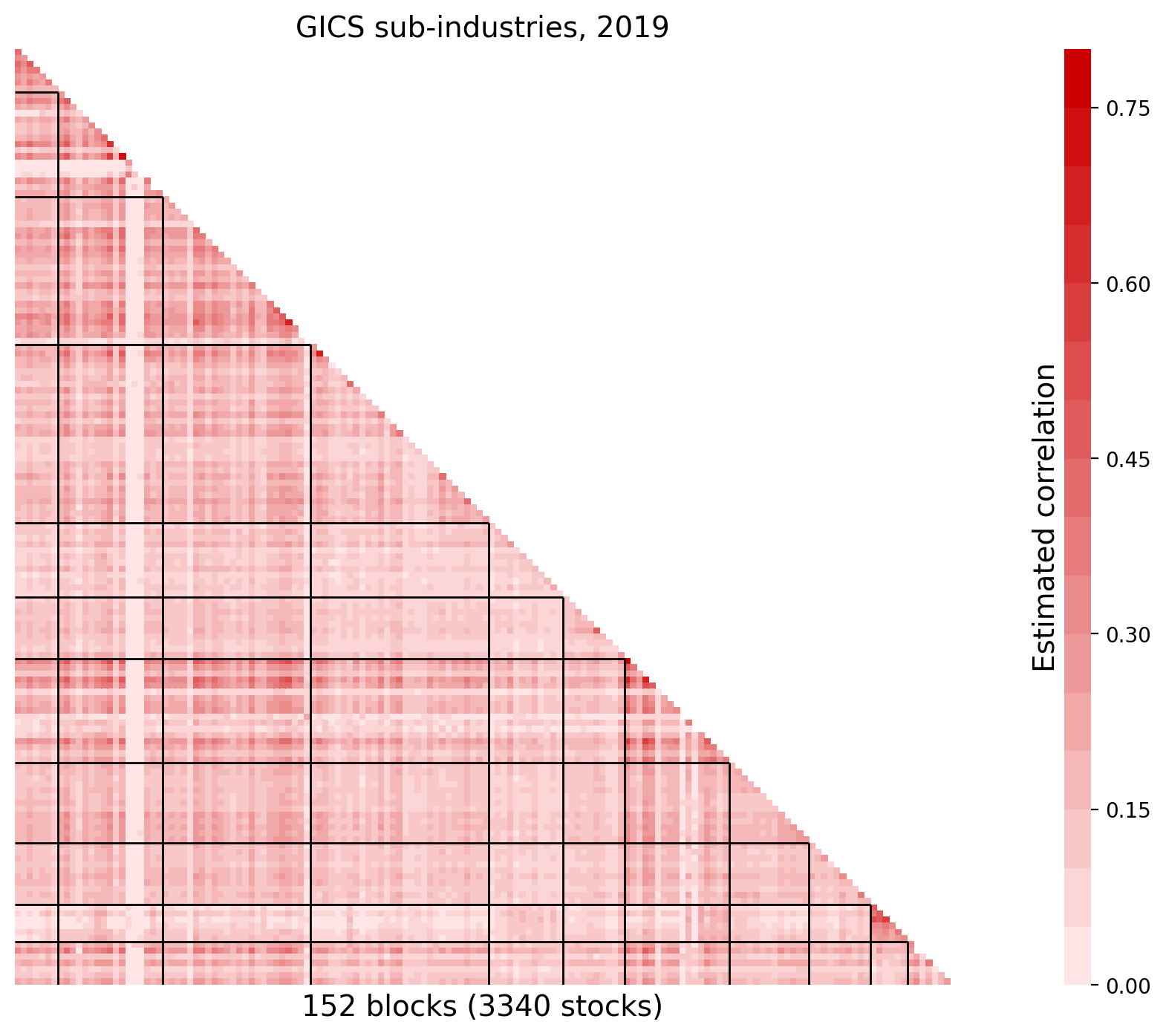
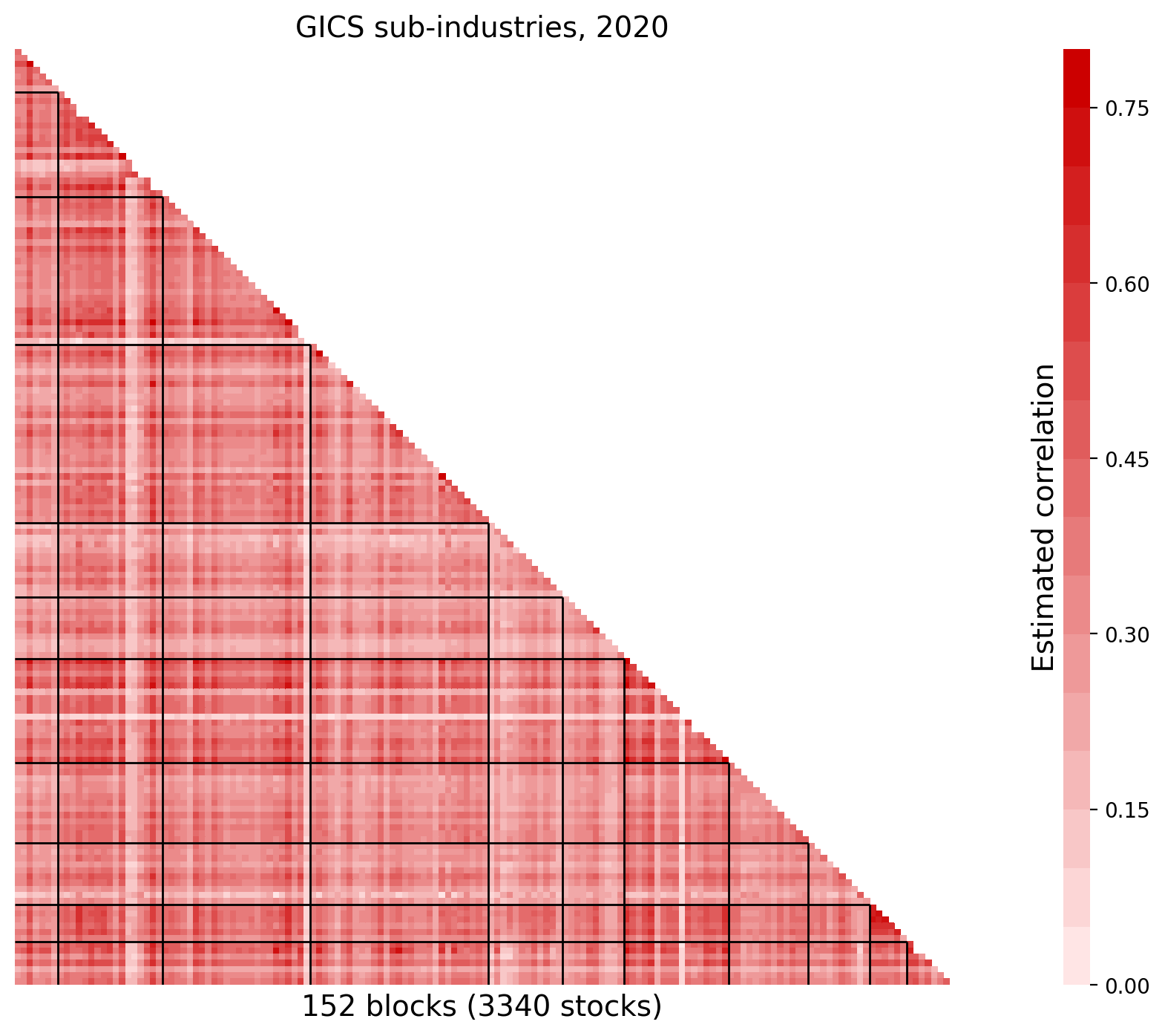
Figure 1: Estimated $3340\times 3340$ block-correlation matrices based on daily returns for 2019 (left) and 2020 (right), where the block structure is define by sub-industries ($K=152$ blocks).

The solid lines indicate the boundaries of the 11 GICS sectors: Energy (10), Materials (15), Industrials (20), Consumer Discretionary (25), Consumer Staples (30), Health Care (35), Financials (40), Information Technology (45), Communication Services (50), Utilities (55), and Real Estate (60). Each of these $3340\times 3340$ correlation matrices are estimate with just 252 vectors of daily returns in 2019 and 253 daily returns in 2020. Correlations were generally larger in 2020 than in 2019. This is not surprising given the impact that the COVID-19 pandemic had on financial markets in 2020. The estimated correlations reveal interesting differences within the sectors and sub-industries (related to gold and other precious metals, biotechnology, and pharmaceuticals) that are largely uncorrelated with other sub-industries. More details are presented in Section 5.

As a preview of our theoretical results, consider the $n\times n$ equicorrelation matrix,

$$C=\left[\begin{array}[]{cccc}1&\rho&\cdots&\rho\\ \rho&1&\ddots&\vdots\\ \vdots&\ddots&\ddots&\rho\\ \rho&\cdots&\rho&1\end{array}\right],$$

which has the eigenvalues, $1+\rho(n-1)$ and $1-\rho$, where the latter has multiplicity $n-1$. This follows directly from the spectral decomposition,

$$Q^{\prime}CQ=D=\left[\begin{array}[]{cc}1+\rho(n-1)&0\\ 0&(1-\rho)I_{n-1}\end{array}\right],$$ (1)

where $Q$ is an orthonormal matrix, i.e., $Q^{\prime}Q=I_{n}$, see Olkin & Pratt (1958). Here $I_{n}$ denotes the $n\times n$ identity matrix. The matrix $Q$ is given by $Q=(v_{n},v_{n\bot})$, where $v_{n}$ is the $n$-dimensional vector, $v_{n}=(\tfrac{1}{\sqrt{n}},\ldots,\tfrac{1}{\sqrt{n}})^{\prime}$, and $v_{n\bot}$ is an $n\times(n-1)$ matrix that is orthogonal to $v_{n}$, i.e., $v_{n\bot}^{\prime}v_{n}=0$, and orthonormal, i.e., $v_{n\bot}^{\prime}v_{n\bot}=I_{n-1}$. It can now be verified that $QQ^{\prime}=I_{n}$ and $C=QQ^{\prime}CQQ^{\prime}=QDQ^{\prime}$. In this example, $D$ is the canonical form of $C$, which is obtained via a rotation of $C$, where the rotation matrix, $Q$, does not depend on $\rho$.

In this paper, we derive a similar decomposition for a broad class of block matrices, which includes block covariance matrices and block correlation matrices as special cases. In the general case with multiple blocks, $K\geq 2$, the canonical representation does not fully disentangle all eigenvalues. The canonical representation decomposes any block matrix into a $K\times K$ matrix and $n-K$ real-valued eigenvalues, where $K$ is the number of blocks. We can illustrate the general results with a $2\times 2$ block correlation matrix,

$$C=\left[\begin{array}[]{c|c}C_{\rho_{11}}&\rho_{12}\mathbf{1}_{n_{1}\times n_{2}}\\ \hline\cr\bullet&C_{\rho_{22}}\end{array}\right]$$

where $C_{\rho_{11}}$ and $C_{\rho_{22}}$ are equicorrelation matrices with correlations $\rho_{11}$ and $\rho_{22}$, respectively, and dimensions $n_{1}\times n_{1}$ and $n_{2}\times n_{2}$, respectively, and $\mathbf{1}_{n_{1}\times n_{2}}$ is the $n_{1}\times n_{2}$ matrix whose elements are all equal to one. Now define

$$Q=\left[\begin{array}[]{cccc}v_{n_{1}}&0&v_{n_{1}\bot}&0\\ 0&v_{n_{2}}&0&v_{n_{2}\bot}\end{array}\right].$$

For this correlation matrix with $2\times 2$ blocks, we have the following representation,

$$Q^{\prime}CQ=\left[\begin{array}[]{cccc}1+\rho_{11}(n_{1}-1)&\rho_{12}\sqrt{n_{1}n_{2}}&0&0\\ \rho_{12}\sqrt{n_{1}n_{2}}&1+\rho_{22}(n_{2}-1)&0&0\\ 0&0&(1-\rho_{11})I_{n_{1}-1}&0\\ 0&0&0&(1-\rho_{22})I_{n_{2}-1}\end{array}\right].$$ (2)

We denote the upper-left $2\times 2$ matrix by $A$. In general, $A$ will be a $K\times K$ matrix, whose eigenvalues are also eigenvalues of $C$. The general result for block matrices with $K$ blocks will be presented in Theorem 1, with a structure similar to that in (2). Importantly, the matrix $Q$ does not depend on the elements in block matrix, but is solely determined by the block partition, $(n_{1},\ldots,n_{K})$, where $n=n_{1}+\cdots+n_{K}$.

The canonical representation is obtained for general block matrices, which need not be symmetric, nor positive semidefinite. In fact, our results are applicable to non-square matrices. Block covariance matrices and block correlation matrices are important special cases. For block correlation matrices, the $A$-matrix, which emerges in (2), was previously established in Huang & Yang (2010) and Cadima et al. (2010), as we will discuss in Section 3. We derive additional results for block correlation matrices that simplify various matrix transformations and the evaluation of the Gaussian log-likelihood function.

The rest of this paper is organized as follows. We present the main result in Section 2, where the canonical representation is established for a broad class of block matrices, along with related results for some matrix functions. We also cover aspects of block structures in regressions with many variables. In Section 3, we consider the special case with block covariance matrices and block correlation matrices. Many of these results are useful for maximum likelihood estimation with a Gaussian log-likelihood function, as we show in Section 4. In Section 5, we present our empirical analysis of block covariance matrices for a large panel of daily stock returns. We conclude in Section 6 and all proofs are presented in the Appendix. A separate Web Appendix with additional empirical results, expressions for computing partial correlations from block correlation matrices, and Matlab code used in our empirical analysis.

2 Canonical Representation of Block Matrices

Let $B$ be a square $n\times n$ matrix. The extension to rectangular matrices is trivial and will be addressed towards the end of this section. The matrix, $B$, is called a block matrix with block partition, $n_{1},\ldots,n_{K}$, if it can be expressed as:

$$B=\left[\begin{array}[]{cccc}B_{[1,1]}&B_{[1,2]}&\cdots&B_{[1,K]}\\ B_{[2,1]}&B_{[2,2]}\\ \vdots&&\ddots\\ B_{[K,1]}&&&B_{[K,K]}\end{array}\right],$$

where $B_{[k,l]}$ is an $n_{k}\times n_{l}$ matrix with the following structure

$$B_{[k,k]}=\left[\begin{array}[]{cccc}d_{k}&b_{kk}&\cdots&b_{kk}\\ b_{kk}&d_{k}&\ddots\\ \vdots&\ddots&\ddots\\ b_{kk}&&&d_{k}\end{array}\right]\quad\text{and }\quad B_{[k,l]}=\left[\begin{array}[]{ccc}b_{kl}&\cdots&b_{kl}\\ \vdots&\ddots\\ b_{kl}&&b_{kl}\end{array}\right]\quad\text{if }k\neq l,$$ (3)

for some constants, $d_{k}$ and $b_{kl}$, $k,l=1,\ldots,K$. So the diagonal elements of the diagonal blocks, $B_{[k,k]}$, can take a different value than the off-diagonal elements, whereas all elements in an off-diagonal block, $B_{[k,l]}$, $k\neq l$, are identical.

We introduce the following notation, which relates to orthogonal projections. Let $P_{[k,l]}=v_{n_{k}}v_{n_{l}}^{\prime}$ be the $n_{k}\times n_{l}$ matrix whose elements are all equal to $\frac{1}{\sqrt{n_{k}n_{l}}}$. It is simple to verify that $P_{[k,m]}P_{[m,l]}=P_{[k,l]}$, and with $k=l=m$ it follows that $P_{[k,k]}P_{[k,k]}=P_{[k,k]}$, such that $P_{[k,k]}$ is a projection matrix. It then follows that $P_{[k,k]}^{\bot}=I_{n_{k}}-P_{[k,k]}$ is a projection matrix, and it can be verified that $P_{[k,k]}^{\bot}=v_{n_{k}\bot}v_{n_{k}\bot}^{\prime}$, where the matrix, $v_{n\bot}$, was characterized in the introduction.

Finally, we define the $n\times n$ matrix

$$Q=\left[\begin{array}[]{cccccccc}v_{n_{1}}&0&\cdots&&v_{n_{1}\bot}&0&\cdots&0\\ 0&v_{n_{2}}&&&0&v_{n_{2}\bot}&&\vdots\\ \vdots&&\ddots&&&&\ddots\\ 0&\cdots&&v_{n_{K}}&0&\cdots&&v_{n_{K}\bot}\end{array}\right],$$

and observe that $Q$ is an orthonormal matrix, characterized by the identity $Q^{\prime}Q=I$. The first $K$ columns of $Q$ can be used to form averages within each of the $K$ blocks, whereas the remaining columns of $Q$ capture “differences” within each block. The two sets of columns span orthogonal subspaces, which correspond to distinct components of the block decomposition. Note that $Q$ is solely defined by the block partition, $n_{1},\ldots,n_{K}$, and it is therefore invariant to the actual values taken by the elements in the block matrix.

Theorem 1.

Suppose that $B$ is a block matrix with block partition $n_{1},\ldots,n_{K}$. Then

$$B_{[k,l]}=a_{kl}P_{[k,l]}+1_{\{k=l\}}\lambda_{k}P_{[k,k]}^{\bot},\qquad\text{for}\quad k,l=1,\ldots,K,$$

where $a_{kl}=b_{kl}\sqrt{n_{k}n_{l}}$, for $k\neq l$, $a_{kk}=d_{k}+(n_{k}-1)b_{kk}$, and $\lambda_{k}=d_{k}-b_{kk}$. Moreover,

$$B=QDQ^{\prime},\qquad\text{with}\quad D=\left[\begin{array}[]{cccc}A&0&\cdots&0\\ 0&\lambda_{1}I_{n_{1}-1}&\ddots&\vdots\\ \vdots&\ddots&\ddots&0\\ 0&\cdots&0&\lambda_{K}I_{n_{K}-1}\end{array}\right],$$ (4)

where $A=\{a_{kl}\}_{k,l=1}^{K}\in\mathbb{R}^{K\times K}$.

The matrix $Q$ rotates $B$ into its canonical form, $D$. The first $K$ columns of $Q$ span the eigenspace of $B$ that is associated with the eigenvalues that $A$ and $B$ have in common. The last $n-K$ columns of $Q$ are the remaining eigenvectors of $B$.

For an arbitrary matrix, $B$, we would not expect $Q^{\prime}BQ$ to have zeroes in particular entries. The block structure imposes a type of sparsity. Rather than imposing the sparsity on $B$, it is imposed on $Q^{\prime}BQ$.

Theorem 1 can be used to characterize properties of $B$ and simplifies the computation of some matrix transformations. These include the matrix exponential, $\exp(B)=\sum_{j=0}^{-\infty}\tfrac{1}{j!}B^{j}$, and the matrix logarithm, denoted $\log B$, which is the inverse of $\exp(B)$. The matrix exponential and matrix logarithm are used in spatial models, see LeSage & Pace (2007), in multivariate volatility models, see e.g., Kawakatsu (2006), Maheu & McCurdy (2011), Asai & So (2015), and Archakov et al. (2020), and play a central role in Markov processes. The matrix logarithm is not always well-defined, but for a positive definite symmetric matrix, $B=V\Lambda V^{\prime},$ where $\Lambda$ is the diagonal matrix with $B$’s eigenvalues, $\xi_{1},\ldots,\xi_{n}$, we simply have $\log B=V\mathrm{diag}(\log\xi_{1},\ldots,\log\xi_{n})V^{\prime}$.

Corollary 1.

Suppose that $B$ is a block matrix as defined above. $(i)$ The eigenvalues of $B$ are the eigenvalues of $A$ and $\lambda_{k}=d_{k}-b_{kk}$, (the latter with multiplicity $n_{k}-1$) $k=1,\ldots,K$, such that $\det B=\det(A)\lambda_{1}^{n_{1-1}}\cdots\lambda_{K}^{n_{K}-1}$. $(ii)$ $B$ is invertible, if and only if $A$ is invertible and $d_{k}\neq b_{kk}$, for all $k=1,\dots,K$. $(iii)$ The $q$-th power of the block matrix, $B^{q}$, is well-defined whenever $A^{q}$ and $\lambda_{k}^{q}$, $k=1,\ldots,K$, are well-defined, in which case $B^{q}$ has the same block structure as $B$, with blocks given by

$$B_{[k,l]}^{q}=a_{kl}^{(q)}P_{[k,l]}+1_{\{k=l\}}\lambda_{k}^{q}P_{[k,k]}^{\bot},$$

where $a_{kl}^{q}$ is the $kl$-th element of $A^{q}$, for $k,l=1,\ldots,K$. $(iv)$ The matrix exponential of $B$ has the same block structure as $B$, with blocks given by

$$\exp(B)_{[k,l]}=a_{kl}^{\exp}P_{[k,l]}+1_{\{k=l\}}e^{\lambda_{k}}P_{[k,k]}^{\bot},$$

where $a_{kl}^{\exp}$ is the $kl$-th element of $\exp A$, for $k,l=1,\ldots,K$. $(v)$ If $\log A$ and $\log\lambda_{k}$, $k=1,\ldots,K$, exist, then $\log B$ has the same block structure as $B$, with blocks given by

$$\log(B)_{[k,l]}=a_{kl}^{\log}P_{[k,l]}+1_{\{k=l\}}\log\lambda_{k}P_{[k,k]}^{\bot},$$

where $a_{kl}^{\log}$ is the $kl$-th element of $\log A$.

It follows that $B^{q}$ is well-defined for all positive integers of $q$, and the matrix inverse, $B^{-1}$, exists whenever $A$ is invertible and $\lambda_{k}\neq 0$, for all $k=1,\ldots,K$, in which case $B^{q}$ is also well-defined for other negative integers of $q$. The logarithms, $\log A$ and $\log(d_{k}-b_{kk})$, exist provided that $A$ is invertible and $d_{k}-b_{kk}\neq 0$. This may result in a complex-valued solution to the matrix logarithm. If a real-valued solution is required, then the conditions are that $A$ is positive definite and that $d_{k}-b_{kk}>0$ for all $k=1,\ldots,K$.

2.1 Block Matrices with Kronecker Representation

Many of the expressions can be simplified further in the special case, where all block sizes are identical, i.e., $n_{1}=n_{2}=\ldots=n_{K}=n$, with $n=N/K$. In this situation, we have $B=A\otimes P+\Lambda\otimes P_{\bot}$, where $P$ is the $n\times n$ matrix with $1/n$ in all entries, $P_{\bot}=I_{n}-P$, and $\Lambda=\mathrm{diag}(\lambda_{1},\ldots,\lambda_{K})$. In this case, it follows that $h(B)=h(A)P+h(\Lambda)P_{\bot}$, where $h(\cdot)$ represents the matrix inverse, the matrix exponential, or the matrix logarithm, provided these are well-defined.

2.2 Rectangular Block Matrices

Suppose that $B$ has blocks, $B_{[k,l]}\in\mathbb{R}^{n_{k}\times n_{l}}$, as specified in (3), where $k=1,\ldots,K_{1}$ and $l=1,\ldots,K_{2}$, and $K_{1}\neq K_{2}$, such that $B$ is a non-square matrix. Set $K=\max(K_{1},K_{2})$ and suppose that $K_{1}>K_{2}$. We conjoin zero-matrix to $B$, such that $\tilde{B}=(B,0)$ is a square matrix with the block partition, $n_{1},\ldots,n_{K}$. Our results apply to $\tilde{B}$, such that $\tilde{B}=QDQ^{\prime}$ has the canonical form and $B=QD\tilde{Q}^{\prime}$, where $\tilde{Q}^{\prime}$ is made up of the first $n_{1}+\cdots+n_{K_{2}}$ columns of $Q^{\prime}$. If $K_{2}>K_{1}$, we can instead define $\tilde{B}=(B^{\prime},0)^{\prime}$, and the results follow similarly. We will make use of rectangular block matrices in the next subsection.

2.3 Application to Regressions with Many Variables

Block matrices can be used to impose structure in regression models with many regressors, many instrumental variables, and many dependent variables. Consider the standard regression model with stationary variables, $Y_{t}=\beta^{\prime}X_{t}+\varepsilon_{t}$, $t=1,\ldots,n$ and $X_{t}\in\mathbb{R}^{q}$. If $q$ is large relative to $n$, it may be desirable to estimate $\Sigma_{xx}=\mathbb{E}[X_{t}X_{t}^{\prime}]$ with a suitable block structure. If $Y_{t}\in\mathbb{R}^{p}$ is also high-dimensional, one might also want to impose a block structure on $\mathbb{E}[X_{t}Y_{t}^{\prime}]$. A similar problem arises in regressions with many instrument, $Z_{t}$, where we can impose a block structure on $\mathbb{E}[X_{t}Z_{t}^{\prime}]$.

Theorem 2.

Suppose that $(X_{t},Z_{t})$ is stationary and ergodic with finite second moment, $X_{t}\in\mathbb{R}^{q}$ and $Z_{t}\in\mathbb{R}^{m}$ with $m\geq q$. Let $\Sigma_{zx}=\mathbb{E}[Z_{t}X_{t}^{\prime}]$ and suppose that $\Sigma_{z\tilde{x}}=[\Sigma_{zx},0_{m\times(m-q)}]$ has a block structure, where $\tilde{X_{t}}=(X_{t}^{\prime},0_{1\times m-q})^{\prime}$. Then $\Sigma_{z\tilde{x}}=QD_{z\tilde{x}}Q^{\prime}$, where the elements of $D_{z\tilde{x}}=\mathrm{diag}(A,\lambda_{1}I_{n_{1}-1},\ldots,\lambda_{K}I_{n_{K}-1})$ can be estimated consistently, as $T\rightarrow\infty$, with

$$\hat{A}=\frac{1}{T}\sum_{t=1}^{T}V_{0,t}W_{0,t}^{\prime}\quad{\color[rgb]{0,0,0}\text{and}}\qquad\hat{\lambda}_{k}=\frac{1}{T}\sum_{t=1}^{T}\tfrac{V_{k,t}^{\prime}W_{k,t}}{n_{k}-1},\quad k=1,\ldots,K,$$

where $V_{t}\equiv Q^{\prime}\tilde{X}_{t}$ and $W_{t}=Q^{\prime}Z_{t}$. The estimate of $\Sigma_{zx}$ is given by the first $q$ columns of $\hat{\Sigma}_{z\tilde{x}}=Q\hat{D}_{z\tilde{x}}Q^{\prime}$.

Theorem 2 is applicable to regression-type estimators, such as the two-stage least squares (TSLS) estimator, $\hat{\beta}_{\mathrm{TSLS}}=[\hat{\Sigma}_{xz}\hat{\Sigma}_{zz}^{-1}\hat{\Sigma}_{zx}]^{-1}[\hat{\Sigma}_{xz}\hat{\Sigma}_{zz}^{-1}\hat{\Sigma}_{zy}]$, where the same, or different, block structures can be imposed on the matrices, $\Sigma_{zx}$, $\Sigma_{zz}$, and $\Sigma_{zy}$.

Imposing a block structure entails a bias-variance trade-off, because the block structure will induce a bias, if $\Sigma_{xz}$ does not have the block structure. Meanwhile, a large reduction in the number of parameters will reduce the variance of the estimator. In this context, the unrestricted estimate, $\frac{1}{T}\sum_{t=1}^{T}Z_{t}X_{t}^{\prime}$, is also consistent, but has a larger estimation error and many other problems, such as those arising with many instrumental variables. It would be interesting to develop formal tests for block structures in order to avoid block structures that are at odds with data. The bias-variance trade-off can motivate shrinkage methods that are based on block structures. For instance, the use of block structures could be combined with regularization methods, such as those in Ledoit & Wolf (2004), as we elaborate on in our concluding remarks.

3 Block Correlation Matrices

A block correlation matrix is characterized by correlation coefficients that form a block structure, where the correlation between two variables is solely determined by the blocks to which the two variables belong.

Block correlation matrices offer a way to parameterize large covariance matrices in a parsimonious manner. This structure is used in some multivariate GARCH models, see Engle & Kelly (2012) and Archakov et al. (2020).

An $n\times n$ block correlation matrix, $C$, with $K$ blocks, is a symmetric block matrix with,

$$C_{[k,k]}=\left[\begin{array}[]{cccc}1&\rho_{kk}&\cdots&\rho_{kk}\\ \rho_{kk}&1&\ddots\\ \vdots&\ddots&\ddots\\ \rho_{kk}&&&1\end{array}\right]\quad\text{and for }k\neq l,\quad C_{[k,l]}=\left[\begin{array}[]{ccc}\rho_{kl}&\cdots&\rho_{kl}\\ \vdots&\ddots\\ \rho_{kl}&&\rho_{kl}\end{array}\right],$$ (5)

where $\rho_{kk}$, $k=1,\ldots,K$ are within-block correlations, and $\rho_{kl}=\rho_{lk}$, $k\neq l$, are between-block correlations, for $k,l=1,\ldots,K$. For $C$ to be a correlation matrix, we obviously need $\rho_{kl}\in[-1,1]$ for all $k,l=1,\ldots,K$, but this is insufficient to guarantee a valid correlation matrix. Negative eigenvalues can arise with some combinations of correlation coefficients, even if these are all strictly smaller than one in absolute value.

Block equicorrelation matrices corresponds to the case where the diagonal elements of all diagonal blocks, $B_{[k,k]}$ equal $d_{k}=1$, for $k=1,\ldots,K$. So, Theorem 1 fully characterizes the set of correlation coefficients that yields a positive (semi-) definite correlation matrix. We formulate this result as a separate Corollary. Note that the canonical form, (4), for $C$ in (5), yields a symmetric $A$ with elements $a_{kl}=\rho_{kl}\sqrt{n_{k}n_{l}}$, for $k\neq l$, $a_{kk}=1+\rho_{kk}(n_{k}-1)$, and $\lambda_{k}=1-\rho_{kk}$.

Corollary 2 (Block correlation matrices).

Let $C$ be a block correlation matrix. Then

$$\det C=\det A\cdot\prod_{k=1}^{K}(1-\rho_{kk})^{n_{k}-1},$$

such that $C$ is a non-singular block correlation matrix if and only if $A$ is positive definite and $|\rho_{kk}|<1$. In this case, both $C^{-1}$ and $\log C$ have the same block structure as $C$, with blocks given by

$$C_{[k,l]}^{-1}=a_{kl}^{\#}P_{[k,l]}+1_{\{k=l\}}\tfrac{1}{1-\rho_{kk}}P_{[k,k]}^{\bot},$$

and

$$\log(C)_{[k,l]}=\tilde{a}_{kl}P_{[k,l]}+1_{\{k=l\}}\log(1-\rho_{kk})P_{[k,k]}^{\bot},$$

respectively, where $a_{kl}^{\#}$ is the $kl$-th element of $A^{-1}$ and $\tilde{a}_{kl}$ is the $kl$-th element of $\log A$.

For $C$ in (5) to be a correlation matrix (possibly singular), we need that $A$ is positive semidefinite and that $|\rho_{kk}|\leq 1$, and Corollary 2 characterizes the set of positive definite block equicorrelation matrices. The additional requirements are that $A$ is positive definite and $|\rho_{kk}|<1$, $k=1,\ldots,K$.

In this context with block correlation matrices, the expression for $A$ was previously obtained in Huang & Yang (2010, proposition 5) and in Cadima et al. (2010, theorem 3.1). Huang & Yang (2010) focused on computational issues, which might explain that their paper is overlooked in much of the literature. Their results add valuable insight about the block-DECO model by Engle & Kelly (2012). For instance, their results provide a simple way to evaluate if a block correlation matrix is positive definite (or semidefinite). The expression for the determinant of a correlation matrix in Corollary 2 is a simple implication of the eigenvalues derived in Huang & Yang (2010) and Cadima et al. (2010), whereas the expressions for the inverse and logarithmically transformed correlation matrices are new, and so is our results on the preservation of block structures for certain matrix functions.

4 Applications of the Canonical Representation to Gaussian Log-Likelihood

In this section, we focus on covariance and correlation matrices for normally distributed random variables. We derive simplified expressions for the corresponding log-likelihood functions, which greatly reduce the computational burden when $n$ is large relative to $K$. We derive the maximum likelihood estimator and provide a simple expression for the first derivatives of the log-likelihood function with respect to the unknown parameters (the scores).

We will follow the conventional notation for covariances and variances, we write $\sigma_{kl}$ in place of $b_{kl}$, $k,l=1,\ldots,K$, and $\sigma_{k}^{2}$ in place of $d_{k}$, $k=1,\ldots,K$. Similarly, for correlation matrices we write $\rho_{kl}$ in place of $b_{kl}$, and have $d_{k}=1$.

The density function for the multivariate Gaussian distribution with mean zero and an $n\times n$ covariance matrix, $\Sigma$, is $f(x)=(2\pi)^{-\frac{n}{2}}(\det\Sigma)^{-\frac{1}{2}}\exp(-\tfrac{1}{2}x^{\prime}\Sigma^{-1}x)$. Suppose that $\Sigma$ has the block structure given by $(n_{1},\ldots,n_{K})$, and let $\Sigma=QDQ^{\prime}$ be its canonical representation. The corresponding log-likelihood function (multiplied by $-2$) can be expressed as

$$-2\ell=n\log 2\pi+\log\det D+X^{\prime}QD^{-1}Q^{\prime}X,$$

where $D=\mathrm{diag}(A,\lambda_{1}I_{n_{1}-1},\ldots,\lambda_{K}I_{n_{K}-1})$, with $\lambda_{k}=\sigma_{k}^{2}-\sigma_{k,k}$, and

$$a_{kl}=\begin{cases}\sigma_{k}^{2}+(n_{k}-1)\sigma_{k,k}&\text{for }k=l,\\ \sigma_{k,l}\sqrt{n_{k}n_{l}}&\text{for }k\neq l.\end{cases}$$

So, if we define $Y=(y_{0}^{\prime},y_{1}^{\prime},\ldots,y_{K}^{\prime})^{\prime}=Q^{\prime}X$, where $y_{0}$ is $K$-dimensional and $y_{k}$ is $n_{k}-1$ dimensional, $k=1,\ldots,K$, then it follows that

$$-2\ell=n\log 2\pi+\log\det A+y_{0}^{\prime}A^{-1}y_{0}+\sum_{k=1}^{K}\left((n_{k}-1)\log\lambda_{k}+\tfrac{y_{k}^{\prime}y_{k}}{\lambda_{k}}\right).$$ (6)

This expression shows that the block structure yields a considerable simplification for log-likelihood evaluation. Instead of inverting the $n\times n$ matrix $\Sigma$ and computing $\det\Sigma$, it suffices to invert the smaller $K\times K$ matrix, $A$, and evaluate $\det A$. Moreover, the maximum likelihood estimator based on a random sample, $X_{1},\ldots,X_{N}$, is easily expressed in terms of the transformed variables, $Y_{1}=Q^{\prime}X_{1},\ldots,Y_{N}=Q^{\prime}X_{N}$, as formulated in the following theorem.

Theorem 3.

Suppose that $X_{t}\sim iidN(0,\Sigma)$, $t=1,\ldots,T$ where $\Sigma$ is a block covariance matrix with block partition, $n_{1},\ldots,n_{K}$. Define the transformed variables, $Y_{t}=Q^{\prime}X_{t}=(y_{0,t}^{\prime},y_{1,t}^{\prime},\ldots,y_{K,t}^{\prime})^{\prime}$, where $y_{0,t}\in\mathbb{R}^{K}$ and $y_{k,t}\in\mathbb{R}^{n_{k}-1}$, $k=1,\ldots,K$.

Then $\hat{\Sigma}=Q\hat{D}Q^{\prime}$ is the maximum likelihood estimator of $\Sigma$, where $\hat{D}=\mathrm{diag}(\hat{A},\hat{\lambda}_{1}I_{n_{1}-1},\allowbreak\ldots,\allowbreak\hat{\lambda}_{K}I_{n_{K}-1})$ with

$$\hat{A}=\frac{1}{T}\sum_{t=1}^{T}y_{0,t}y_{0,t}^{\prime}\quad\text{and}\qquad\hat{\lambda}_{k}=\frac{1}{T}\sum_{t=1}^{T}\tfrac{y_{k,t}^{\prime}y_{k,t}}{n_{k}-1},\quad k=1,\ldots,K.$$

The maximum likelihood estimates of the individual parameters can be obtained directly from $\hat{A}$ and $\hat{\lambda}_{k}$, $k=1,\ldots,K$. From the definition of $A$ it follows that $\hat{\sigma}_{k,l}=\hat{a}_{kl}/\sqrt{n_{k}n_{l}}$ for $k\neq l$, and for $k=l$, we have $\hat{\sigma}_{k,k}=(\hat{a}_{kk}-\hat{\lambda}_{k})/n_{k}$ and $\hat{\sigma}_{k}^{2}=\hat{\lambda}_{k}+\hat{\sigma}_{k,k}=\tfrac{1}{n_{k}}\hat{a}_{kk}+\tfrac{n_{k}-1}{n_{k}}\hat{\lambda}_{k}$.

In the special case where a block has size one, we have $\Sigma_{[k,k]}=\sigma_{k}^{2}$ and $\sigma_{k,k}$ is undefined. In this situation, the corresponding, $y_{k,t}$, is also undefined, and hence, so is $\hat{\lambda}_{k}$. Yet the expressions for the maximum likelihood estimators continue to be valid, including the expression for $\hat{\Sigma}$ in Theorem 3. If $n_{k}=1$, then $\hat{\sigma}_{k}^{2}=\hat{a}_{kk}$, while the expression for $\hat{\sigma}_{k,k}$ is redundant and can be ignored.

Estimation when the correlation matrix is assumed to have a block structure, as opposed to the covariance matrix having a block structure, is more convoluted. A block correlation matrix is entirely given by the $A$-matrix, because the eigenvalues $\lambda_{1},\ldots,\lambda_{K}$ are given from $A$. Below we use the notation, $\mathcal{I}_{k}\equiv\{i_{k-1}+1,\ldots,i_{k}\}$, with $i_{k}=\sum_{j=1}^{k}n_{j}$, which contains the $n_{k}$ indices associated with the $k$-th block.

Corollary 3.

Suppose that $X_{t}\sim iidN_{n}(0,\Sigma)$, $t=1,\ldots,T$, where $\Sigma=\Lambda_{\sigma}C\Lambda_{\sigma}$ with $\Lambda_{\sigma}=\mathrm{diag}(\sigma_{1},\ldots,\sigma_{n})$ and $C$ is a block correlation matrix with block partition, $n_{1},\ldots,n_{K}$. The maximum likelihood estimates of $\sigma_{1}^{2},\ldots,\sigma_{n}^{2}$ satisfy

$$\frac{1}{n_{k}}\sum_{i\in\mathcal{I}_{k}}\frac{s_{i}^{2}}{\tilde{\sigma}_{i}^{2}}=1,\qquad k=1,\ldots,K,$$ (7)

where $s_{i}^{2}=T^{-1}\sum_{t=1}^{T}X_{i,t}^{2}$, for $i=1,\ldots,n$. Let $\tilde{X}_{i,t}=X_{i,t}/\tilde{\sigma}_{i}$ and define $\tilde{Y}_{t}=Q^{\prime}\tilde{X}_{t}=(\tilde{y}_{0,t}^{\prime},\tilde{y}_{1,t}^{\prime},\ldots,\tilde{y}_{K,t}^{\prime})^{\prime}$ where $\tilde{y}_{0,t}\in\mathbb{R}^{K}$ and $\tilde{y}_{k,t}\in\mathbb{R}^{n_{k}-1}$, $k=1,\ldots,K$.

The maximum likelihood estimator of $C$ is $\tilde{C}=Q\tilde{D}Q^{\prime}$, where $\tilde{D}=\mathrm{diag}(\tilde{A},\tilde{\lambda}_{1}I_{n_{1}-1},\allowbreak\ldots,\allowbreak\tilde{\lambda}_{K}I_{n_{K}-1})$ with

$$\tilde{A}=\frac{1}{T}\sum_{t=1}^{T}\tilde{y}_{0,t}\tilde{y}_{0,t}^{\prime}\quad\text{and}\qquad\tilde{\lambda}_{k}=\frac{n_{k}-\tilde{a}_{kk}}{n_{k}-1},\quad k=1,\ldots,K,$$

where $\tilde{a}_{kk}$ is the $k$-th diagonal element of $\tilde{A}$.

Thus, the estimate of $D$ can be obtained solely from the $K\times K$ matrix $\tilde{A}$. For the individual correlations we have $\tilde{\rho}_{k,l}=\tilde{a}_{kl}/\sqrt{n_{k}n_{l}}$, for $k\neq l$, and $\tilde{\rho}_{k,k}=(\tilde{a}_{kk}-1)/(n_{k}-1)$, for $k=l$. Corollary 3 does not fully specify the maximum likelihood estimates of $(\sigma_{1}^{2},\ldots,\sigma_{n}^{2})$, but these are given in the proof in implicit form, and some additional details are stated immediately after the proof.

A simple and consistent estimator, as $T\rightarrow\infty$, is to set $\hat{\sigma}_{i}^{2}=s_{i}^{2}$, $i=1,\ldots,n$, which satisfy (7), and compute the corresponding $\hat{C}$, with the expression for $A$ and $\lambda_{k}$, $k=1,\ldots,K$, which maximizes the log-likelihood function subject to $\sigma_{i}^{2}=s_{i}^{2}$, $i=1,\ldots,n$. We refer to this estimator as the two-stage estimator.

The score of the log-likelihood function is often of separate interest. For instance, the score is used for the computation of robust standard errors, in Lagrange multiplier tests, in tests for structural breaks, see e.g., Nyblom (1989), and in dynamic models with time-varying parameters (the so-called score-driven models), see Creal et al. (2013). So we provide the expressions for the score in this context with a block covariance matrix.

Suppose that $\Sigma$ is a block covariance matrix and let $\Sigma=QDQ^{\prime}$ be its canonical representation. Because $Q$ is entirely given by the block partition $(n_{1},\ldots,n_{K})$, and does not depend on the unknown parameters in $\Sigma$, the expressions for the partial derivatives are relatively simple.

Proposition 1.

Let $\Sigma=QDQ$ be the canonical representation of $\Sigma$. Then $\partial(-2\ell)/\partial A=M=A^{-1}-A^{-1}y_{0}y_{0}^{\prime}A^{-1}$ and, for $k=1,\ldots,K$, we have

$$\frac{\partial(-2\ell)}{\partial\sigma_{k}^{2}} = M_{k,k}+\left(\tfrac{n_{k}-1}{\lambda_{k}}-\tfrac{y_{k}^{\prime}y_{k}}{\lambda_{k}^{2}}\right)$$

$$\frac{\partial(-2\ell)}{\partial\sigma_{kk}} = (n_{k}-1)M_{k,k}-\left(\tfrac{n_{k}-1}{\lambda_{k}}-\tfrac{y_{k}^{\prime}y_{k}}{\lambda_{k}^{2}}\right),$$

and, for $i\neq j$, we have $\frac{\partial(-2\ell)}{\partial\sigma_{ij}}=2\sqrt{n_{k}n_{l}}M_{i,j}.$

The hessian could be derived similarly. In some applications, it might be preferable to parametrize the block covariance matrix with $A$ and ($\lambda_{1},\ldots,\lambda_{K})$. In this case, one can use $\partial(-2\ell)/\partial A=M$, and $\partial(-2\ell)/\partial\lambda_{k}=\tfrac{n_{k}-1}{\lambda_{k}}-\tfrac{y_{k}^{\prime}y_{k}}{\lambda_{k}^{2}}$, for $k=1,\ldots,K$.

5 Empirical Estimation of Block Correlation Matrices

We proceed to illustrate how high-dimensional covariance matrices with a block structure are straightforward to estimate in practice. We estimate block correlation matrices for a large panel of daily asset returns for each of the years from 1995 to 2020. We include all stocks from the Center for Research in Security Prices (CRSP) database that could be matched with a unique permanent number (PERMNO from the Compustat data). Stocks with missing observations in a calendar year were excluded from the estimation in that calendar year. Across years, we have between $n=3,340$ and $n=6,637$ stocks, with an average of 4,446 stocks per year. Each calendar year has $T\simeq 250$ daily returns, which we use to estimate the $n\times n$ correlation matrix for that year.

The objective of this empirical application is to demonstrate that high-dimensional covariance matrices can be estimated with relatively few observations once a block structure is imposed, and that the canonical representation makes it simple to obtain consistent estimates and evaluate the Gaussian log-likelihood function. Because variances and covariances vary over time, our estimates reflect correlations implied by the average covariance matrices over each calendar year, rather than an accurate description of the data generating process.

In our analysis, we inspect five nested block structures for the correlation matrix, where the equicorrelation structure ($K=1$) is the simplest and most restrictive model. The other four correlation models use block structures defined by GICS Sectors, Groups, Industries, and Sub-Industries. The numbers of blocks are increasing from Sectors to Sub-Industries, but may change from year to year within a given category. These correspond to $K=11$ for Sectors, and across years $K$ ranges between 24 and 26 for Groups, between 69 and 76 for Industries, and between 152 and 182 for Sub-Industries.

We estimate the canonical correlation matrix for each calendar year using the two-stage estimator. Hence, the individual variances are estimated with the sample variances, $\hat{\sigma}_{i}^{2}=T^{-1}\sum_{t=1}^{T}r_{i,t}^{2}$, where the daily returns, $r_{i,t}$, are adjusted for dividends and stock splits. Then the block correlation matrix is estimated from standardized returns, $\hat{z}_{i,t}=r_{i,t}/\hat{\sigma}_{i}$, using Corollary 3, and we obtain $\hat{\rho}_{k,l}=\hat{a}_{kl}/\sqrt{n_{k}n_{l}}$, for $k\neq l$, and $\hat{\rho}_{k,k}=(\hat{a}_{kk}-1)/n_{k}$, where $\hat{A}=\frac{1}{T}\sum_{t=1}^{T}\hat{y}_{0,t}\hat{y}_{0,t}^{\prime}$ and the $k$-th element of $\hat{y}_{0,t}$ is given by $\frac{1}{\sqrt{n_{k}}}\sum_{i\in\mathcal{I}_{k}}\hat{z}_{i,t}$. So, the entire $n\times n$ covariance matrix with the block correlation structure is estimated by $n$ (univariate) variances and the $K\times K$ matrix, $\hat{A}$. The unrestricted estimate would obviously be singular because the dimension, $n$, is an order of magnitude larger than $T$ in all calendar years. The block assumption imposes enough structure for $\hat{C}$ to be invertible, which requires an inverse of the $K\times K$ matrix, $\hat{A}$.

	Summary statistics of estimated block correlations									# blocks
Block	Mean	Std.	Min	$Q_{10\%}$	$Q_{50\%}$	$Q_{90\%}$	Max	$-\frac{2\ell}{nT}$	$\frac{1}{nT}$BIC	$K$	$\frac{K(K+1)}{2}$
structure
	U.S. market in 2019 (3340 stocks and 252 days)
Equicorrelation	0.138	0	0.138	0.138	0.138	0.138	0.138	2.69177	2.69178	1	1
Sectors	0.134	0.062	-0.002	0.072	0.127	0.208	0.407	2.64243	2.64349	11	66
Groups	0.135	0.052	-0.002	0.080	0.129	0.201	0.407	2.62892	2.63378	24	300
Industries	0.137	0.063	-0.059	0.074	0.129	0.212	0.594	2.61240	2.65152	69	2415
Sub-industries	0.143	0.082	-0.147	0.058	0.133	0.247	0.789	2.57997	2.76832	152	11628
	U.S. market in 2020 (3340 stocks and 253 days)
Equicorrelation	0.298	0	0.298	0.298	0.298	0.298	0.298	2.48686	2.48687	1	1
Sectors	0.317	0.079	0.191	0.223	0.318	0.415	0.639	2.41314	2.41421	11	66
Groups	0.309	0.071	0.153	0.212	0.312	0.395	0.639	2.39740	2.40224	24	300
Industries	0.327	0.083	0.134	0.220	0.321	0.433	0.763	2.37039	2.40938	69	2415
Sub-industries	0.329	0.112	-0.018	0.191	0.324	0.472	0.913	2.32680	2.51444	152	11628

Table 1: Summary statistics for the estimated block correlation matrices.

To conserve space, we only provide the most detailed estimation results for the last two calendar years, 2019 and 2020, and partial correlations will be presented for six calendar years. Detailed results for all 26 calendar years (1995-2018) are presented in the Web Appendix, Archakov & Hansen (2021b). Comparing 2019 and 2020 is interesting because some effects of the COVID-19 pandemic can be observed in 2020. Both years have the same number of assets, $n=3,340$ assets, and the same number of blocks for all five block structures.

In Table 1, we report the range of estimated correlations for each of the five types of block structure and for both calendar years, 2019 and 2020. The range of estimated correlations was larger in 2020 than in 2019, and it increases as the number of blocks increases. The latter is expected because the number of distinct correlation coefficients in $C$ increases as $K$ increases. Each estimated correlation represents an average correlation, subject to both time averaging (over a calendar year) and cross-sectional averaging within the corresponding sector/group/industry/sub-industry. We also report the log-likelihood function (scaled by $-2/(nT)$) evaluated at the parameter estimates, and the corresponding value of the Bayesian Information Criterion (BIC). The minimum BIC is obtained with a block structures based on Groups in both 2019 and 2020. The last column reports the number $K(K+1)/2$ of unique correlations within a block structure with $K$ blocks, and while this number increases rapidly with $K$, the gains in the log-likelihood are relatively modest. Consequently, the BIC increases substantially when blocks are defined by sub-industries.

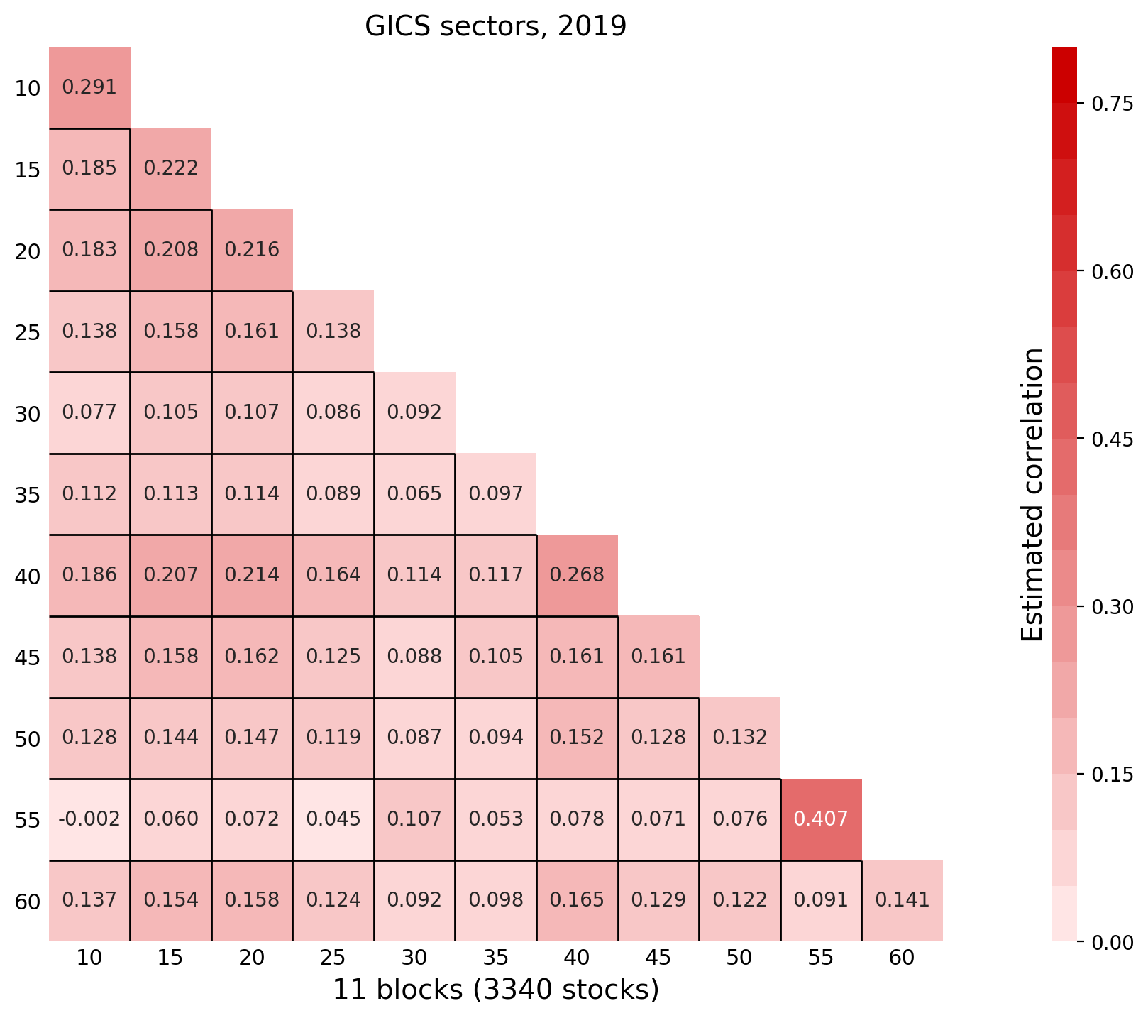
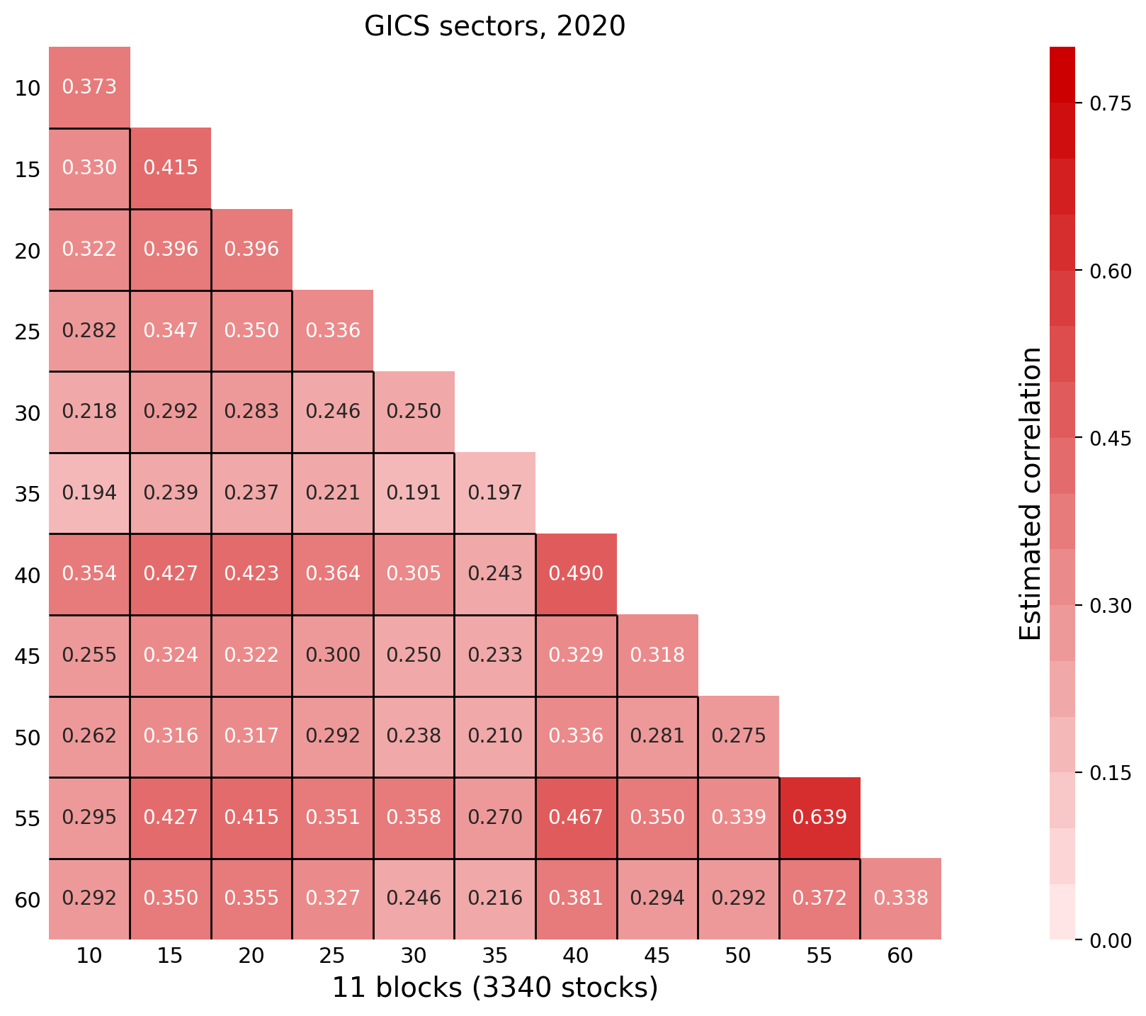
(a) Sector correlation structure ($K=11$ blocks)

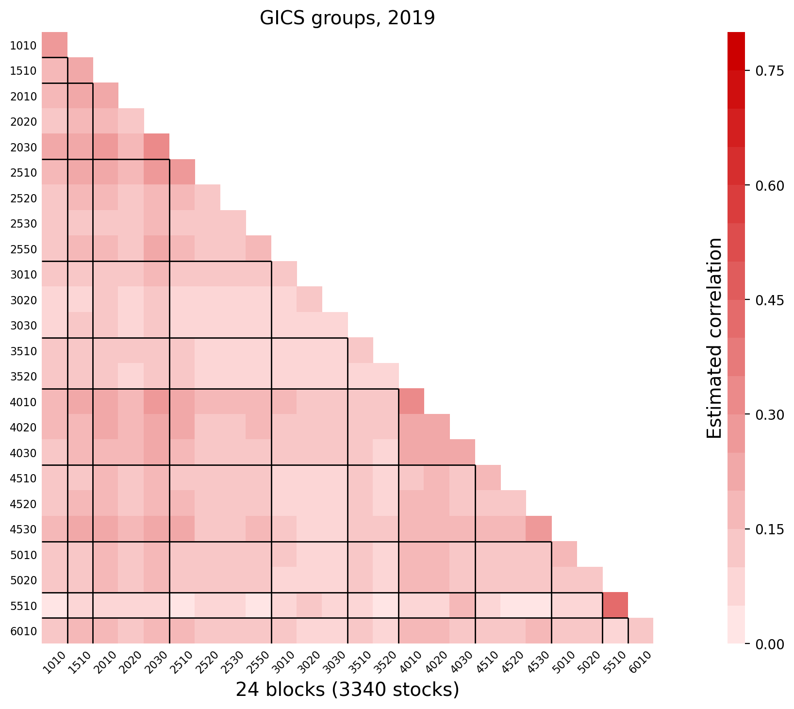
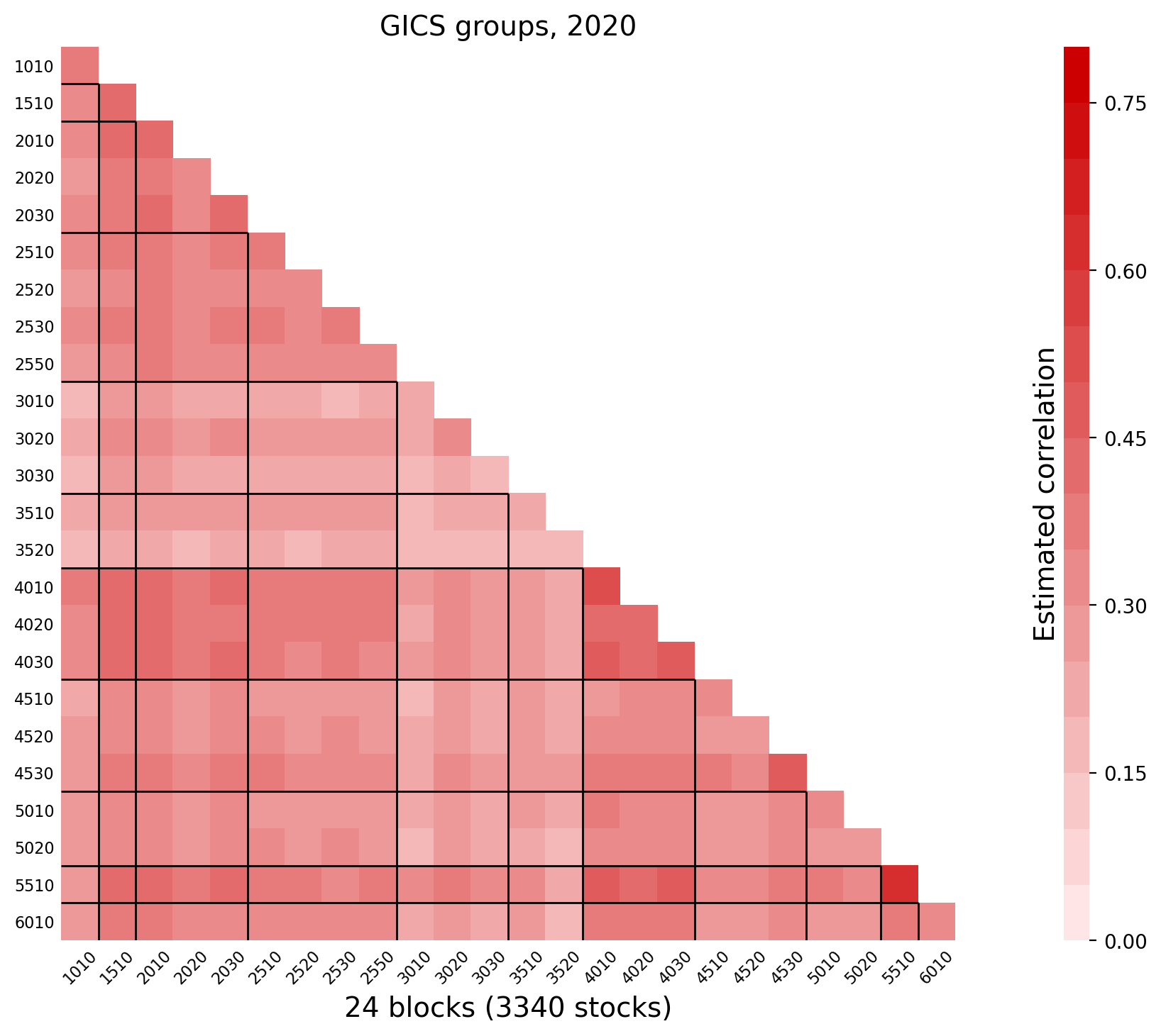
(b) Group correlation structure ($K=24$ blocks)

Figure 2: Estimated correlations for block structure based on Sectors (a), Groups (b), Industries (c) and Sub-industries (d). Left panels are the estimates for 2019 based on 252 daily returns and the right panels are for 2020 based on 253 daily returns from 2020. The block of asset are listed according to their GICS classification code, and the black solid lines indicated the boundaries of the 11 sectors.

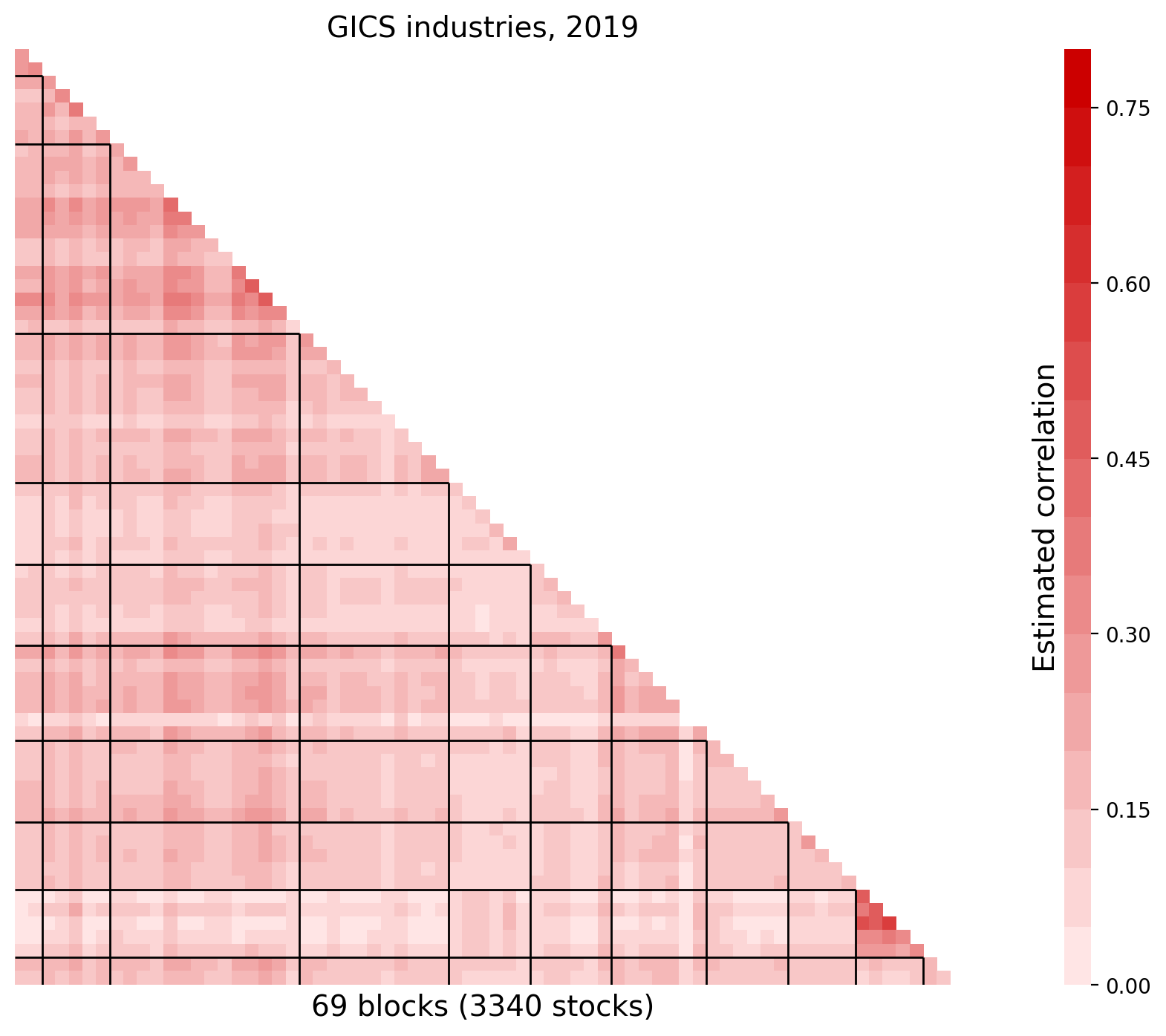
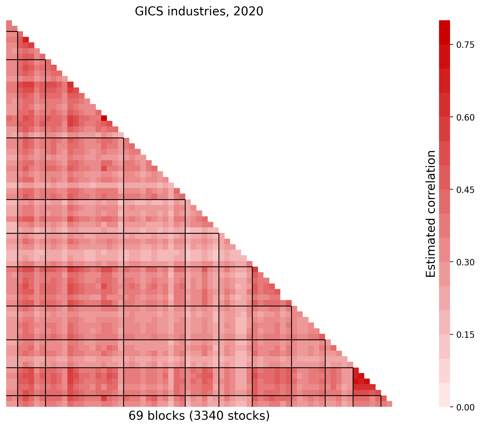
(c) Industry correlation structure ($K=69$ blocks)

(d) Sub-industry correlation structure ($K=152$ blocks)

Figure 2: (continued).

The estimated block correlation matrices based on Sectors, Groups, Industries and Sub-industries are shown in Figure 2. Along the diagonal are the estimated correlation coefficients for assets in the same block (within block correlations). Other estimates are for pairs of assets from different blocks (between block correlations). Due to the larger number of estimated correlation coefficients, we present most estimates using color coding. A darker shade of red denotes a stronger correlation.

From Figure 2 we can see that correlations were generally higher in 2020 than in 2019. This can be attributed to the COVID-19 Pandemic. When COVID-19 cases began to spread worldwide, beyond isolated cases, the market experienced a large decline that continued as lockdowns were imposed in most countries. The S&P 500 index declined by more than 33% from February 19, 2020 to March 23, 2020. This was followed by a strong rally where the market, from March 23, 2020 to the end of the year, increased by more than 63%. The block structure is somewhat more visible in 2020, which could be due to the differentiated effect the pandemic had on different sectors of the economy. For instance, in Figure 2 we can see that the correlation between Utilities (55) and other sectors increased substantially. Finance (40) tended to have the highest average correlation with other sectors, but Utilities (55) had the highest average correlation with other sectors in 2020. The low correlation between Health Care (35) and other sectors is also very pronounced in 2020. The blocks are listed in order of their GICS codes and we include solid black lines to separate different sectors (the number of blocks is too large to include labels for Industries and Sub-Industries individually). The block partition based on Sub-Industries in panel (d) reveals additional details about the correlation structure. Within the Health Care sector (35) there is a distinct stripe that signifies near zero correlations with all other blocks. Interestingly, this stripe corresponds to two subindustries, Biotechnology (35201010) and Pharmaceuticals (35202010). In the Figure 2(d) there is also a band with low correlations that is associated with sub-industries in Materials (15), and these are Gold (15104030), Precious Metals and Minerals (15104040), and Silver (15104045).

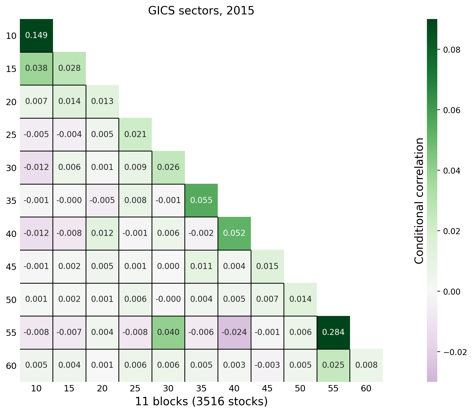
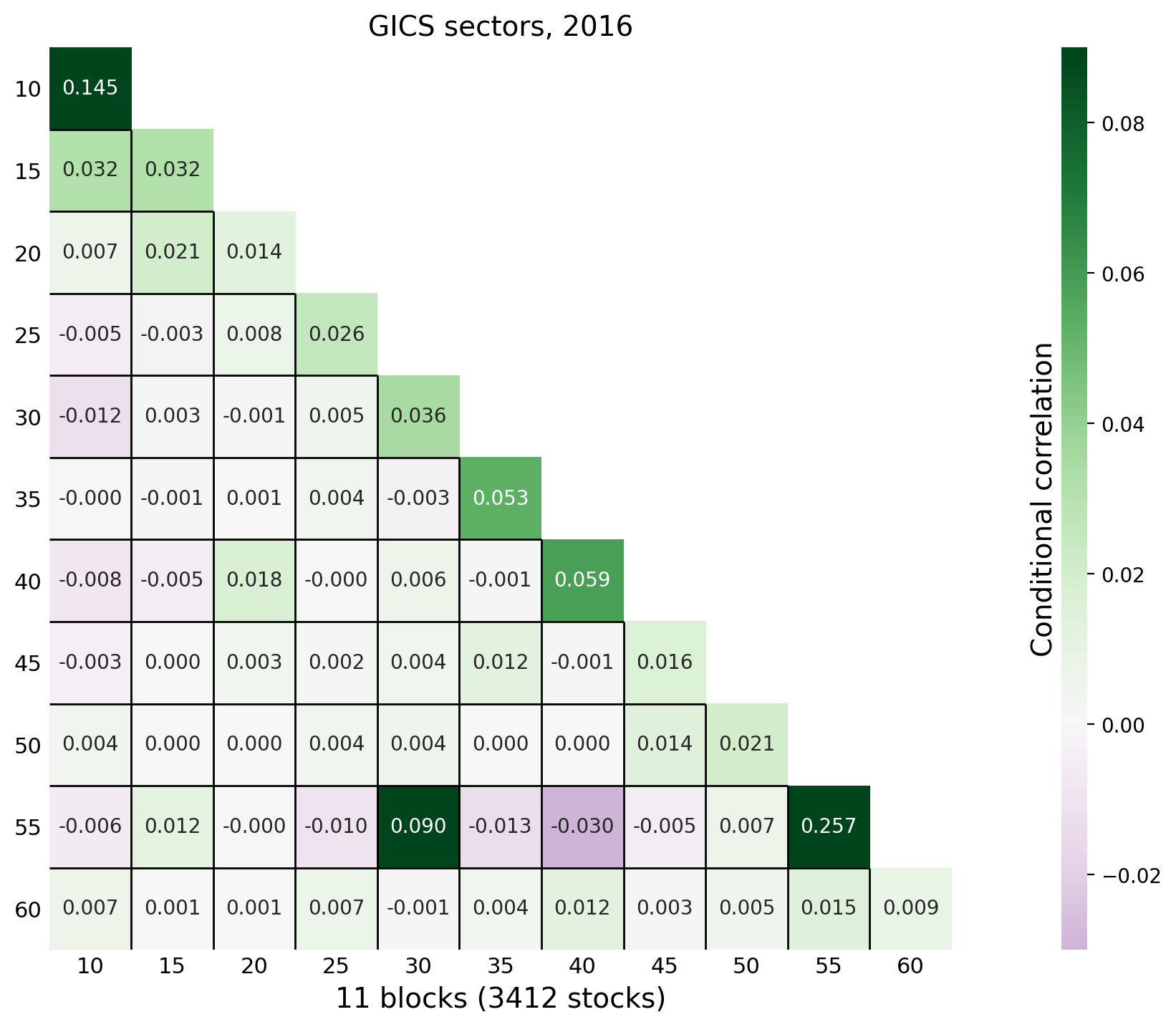
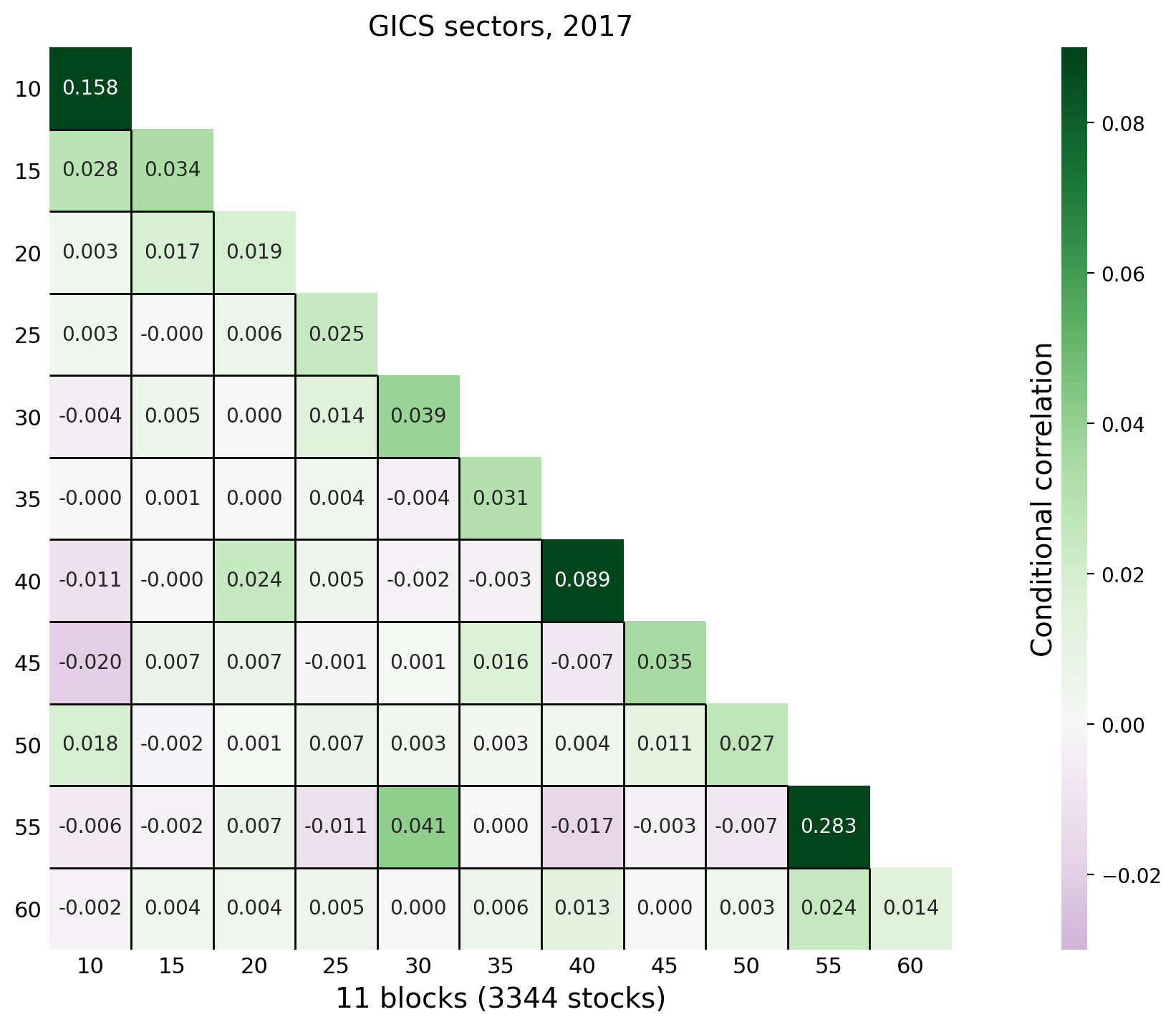
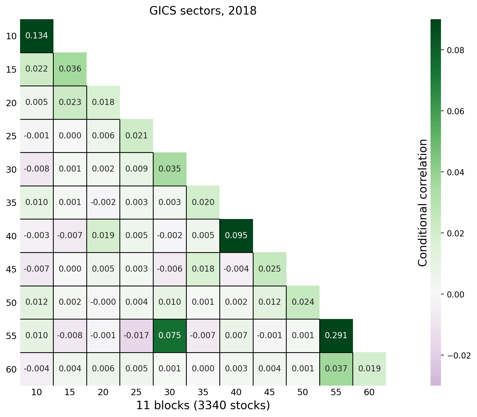
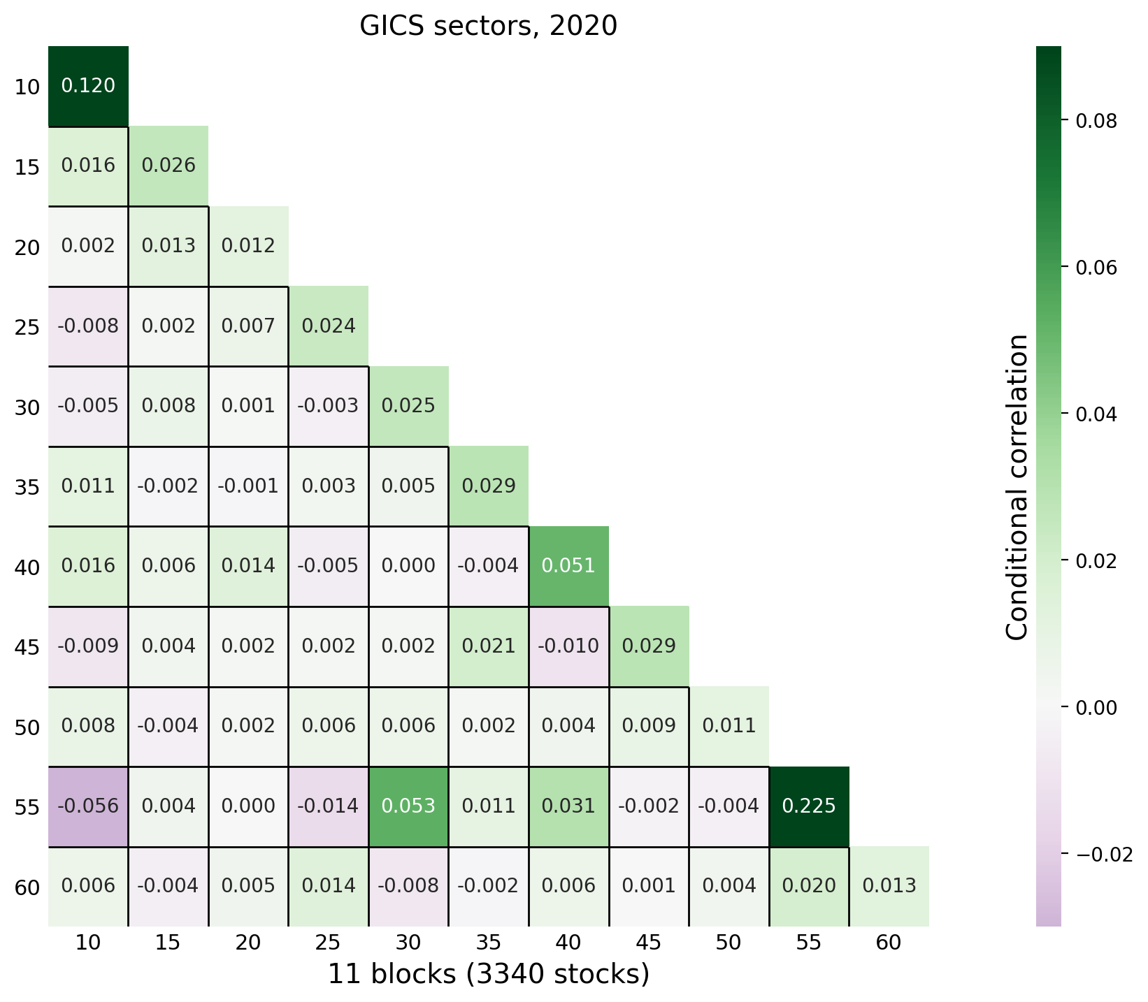
Figure 3: Partial correlations for sector-block correlation matrix by calendar year (2015 - 2020).

To further illustrate the usefulness of the block correlation structure, we compute partial correlations for pairs of stocks. Partial correlations require inversion of a high-dimensional matrix, a computation that is greatly simplified with the block structure. In Figure 3 we report the partial correlation for a pair of stocks, where we have conditioned on all other stocks in other sectors. These partial correlations are based on the estimated correlation matrices using the sector-block structure. Figure 3 includes results for six calendar years, the results for all other calendar years are presented in the Web Appendix.

One feature that stands out from the partial correlation matrices is the similarity across calendar years, of which six years are shown in Figure 3. Had the annual estimates of the correlation matrices been very noisy, we would not expect to see very similar structures in estimates based on different data sets (daily returns from different calendar years). The estimate from one calendar year, tend to be similar to that of the neighboring years, with some exceptions associated with the Global Financial Crisis and the COVID-19 pandemic. This is precisely what we would expect if the correlation structure is time-varying but typically evolves in a relatively smooth manner. It is interesting that two sectors, Energy and Utilities, have large degrees of residual correlation that are left unexplained after having conditioned on all stocks in other sectors. This indicates that these sectors need a sector specific factor to explain their correlation structure. A potentially interesting application of the partial correlation analysis, would be to extend the set of assets with a set of “factors”, such as the three Fama-French factors, and other candidate factors. Computing partial correlations, where the conditioning is on the factors, could be used to identify correlation structures that are left unexplained by the factors. We leave this for future research.

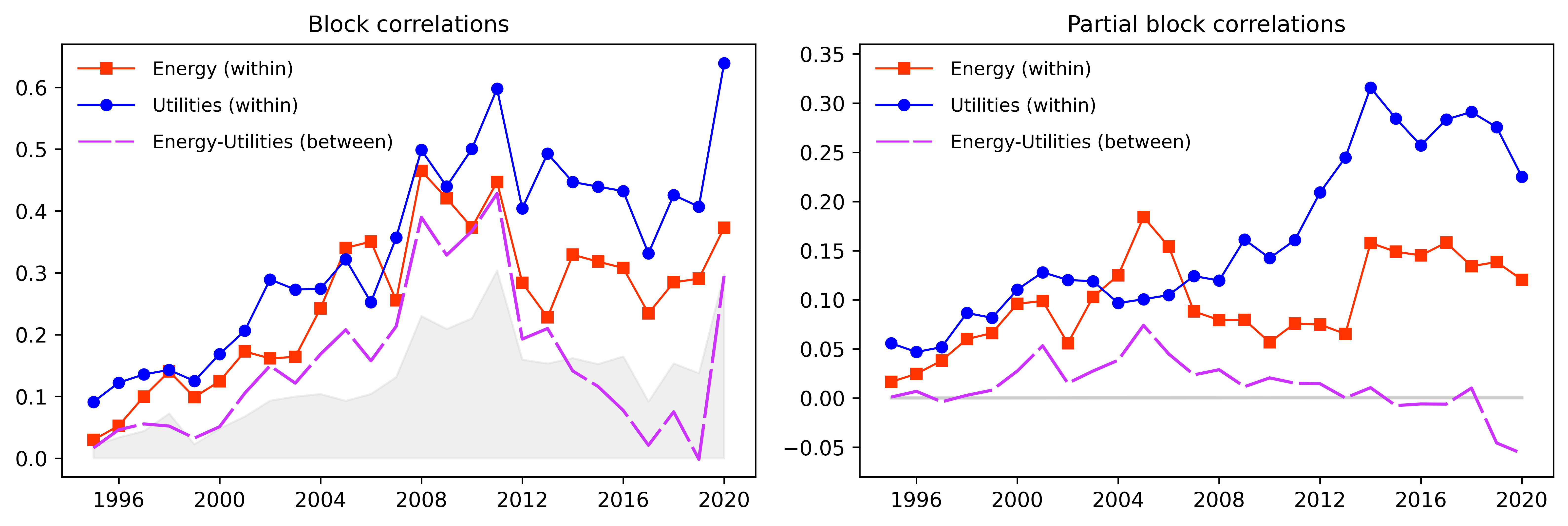
(a) Correlations and Partial Correlations for stock in Energy and Utilities sectors

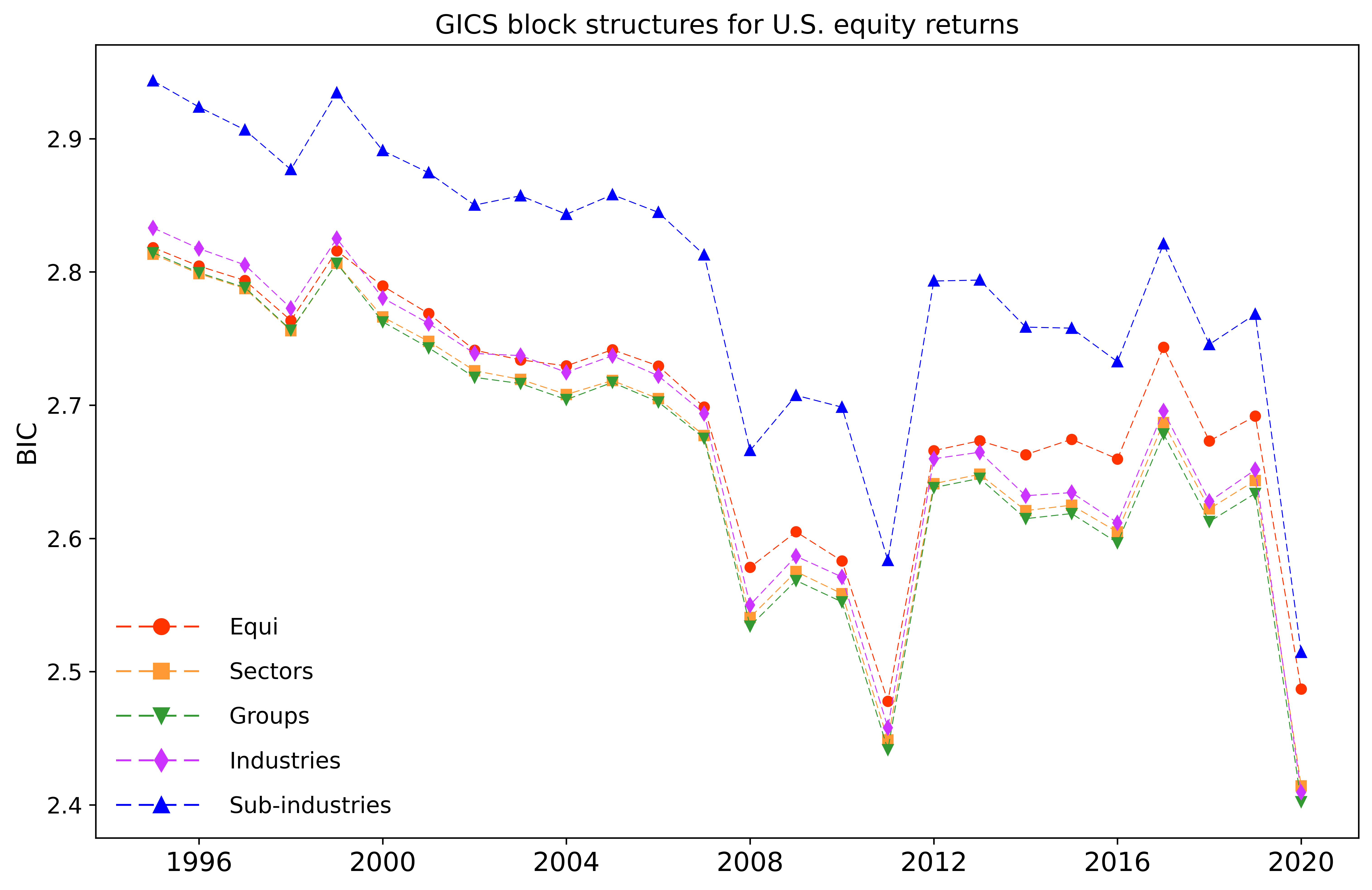
(b) Bayesian Information Criterion (BIC)

Figure 4: Some selected empirical results for all calendar years.

Figure 4 presents selected results for all 26 calendar years. In the upper panel (a), we present the estimated correlations (left) and partial correlations (right) between assets in the Energy and Utilities based on the sector-block structure. The shaded areas represent the average correlation and average partial correlation based on the equicorrelation structure for all assets. Figure 4 shows that the correlations have been trending upwards and there has also been a great deal of variation in the correlation between these two sectors. The partial correlations are interesting, because they indicate that these two sectors, Energy and Utilities, have large idiosyncratic components, because a large fraction of the correlations between stocks within either of these two sectors is unexplained by the thousands of stocks in other sectors.

In the lower panel (b) of Figure 4, we present the BIC for each of the calendar years and each block structure. Before 2000, the BIC always selected the block structures based on sectors and after 2000 it systematically favors the block structure based on Groups. The most heavily parametrized specification, which is based on sub-industries, has the worst BIC in all calendar years.

6 Concluding Remarks

We have derived a canonical representation of block matrices. The representation provides valuable simplifications for models with block matrices, such as stochastic block models for large networks, and models with block covariance and block correlation matrices. We derived a number of expressions that greatly simplify the computation of the Gaussian log-likelihood function with block covariance/correlation matrices. We illustrated this in an empirical application, where we estimate large covariance matrices for a vector with thousands of assets, with daily returns over a single calendar year. Inverting the covariance matrix, computing partial correlations, and evaluating the Gaussian log-likelihood is straightforward once a block structure is imposed.

The canonical representation and the related results are potentially useful for regularizing large covariance matrices. For instance, one could shrink the sample correlation matrix towards a block correlation matrix, analogous to the way Ledoit & Wolf (2004) proposed to shrink towards the equicorrelation matrix with the MacGyver method, see also Engle (2009). This could possibly be extended to shrinkage involving a convex combination of several block correlation matrices.

The canonical representation also paves new ways to testing block structures in covariance and correlation matrices. This predominantly amounts to testing a large number of zero-restrictions in the canonical representation. We identified a number of transformations that preserves the block structures, so testing of block structures could be based on any of the transformations, rather than the original matrix. For instance, block structures in a correlation matrix $C$ would be tested on the canonical representation for $\log C$. This is potentially interesting, because the connection between logarithmically transformed correlation matrix and the Fisher transformation, see Archakov & Hansen (2021a). Finally, the group assignments, and hence $K$, will be unknown in many empirical applications. The literature has therefore proposed various classification methods to determine an appropriate block structure. It is possible that the canonical representation will be useful for this type of classification problems.

Appendix of Proofs

Proof of Theorem 1. For $k\neq l$, we have $B_{[k,l]}=a_{kl}P_{[k,l]}$ if $a_{kl}=b_{kl}\sqrt{n_{k}n_{l}}$, since the elements of $P_{[k,l]}$ are all equal to $\frac{1}{\sqrt{n_{k}n_{l}}}.$ For $k=l$, the diagonal elements differ from off-diagonal elements by $\lambda_{k}=d_{k}-b_{kk}$, so that $B_{[k,k]}=b_{kk}n_{k}P_{[k,k]}+(d_{k}-b_{kk})I_{n_{k}}$. Since $I_{n_{k}}=P_{[k,k]}+P_{[k,k]}^{\bot}$, we have $B_{[k,k]}=(b_{kk}n_{k}+d_{k}-b_{kk})P_{[k,k]}+(d_{k}-b_{kk})P_{[k,k]}^{\bot}=a_{kk}P_{[k,k]}+\lambda_{k}P_{[k,k]}^{\bot}$. The canonical representation, (4), follows by verifying that $Q^{\prime}BQ$ is equal to the block-diagonal matrix in (4). This follows from the identities: $v_{n_{k}}^{\prime}P_{[k,l]}v_{n_{l}}=1$, $v_{n_{k}}^{\prime}P_{[k,l]}v_{n_{l}\bot}=0$, $v_{n_{k}\bot}^{\prime}P_{[k,l]}v_{n_{l}\bot}=0$, $v_{n_{k}}^{\prime}P_{[k,k]}^{\bot}v_{n_{k}}=0$, $v_{n_{k}}^{\prime}P_{[k,k]}^{\bot}v_{n_{k}\bot}=0$, and $v_{n_{k}\bot}^{\prime}P_{[k,k]}^{\bot}v_{n_{k}\bot}=I_{n_{k}-1}$, and the fact that $Q^{\prime}Q=I_{n}$, so that $Q^{-1}=Q^{\prime}$, and hence $B=QQ^{\prime}BQQ^{\prime}$. This proves (4). $\square$

Proof of Corollary 1. The first result for the eigenvalues of $B$ and the determinant of $B$, follows immediately from (4). The results for $f(B)$, where $f$ denotes the $q$-th power of a matrix, the matrix exponential, or the matrix logarithm, follow by $f(B)=Qf(D)Q^{\prime}$ and using the structure in $Q$, such as $v_{n_{k}}v_{n_{l}}^{\prime}=P_{[k,l]}$ and $v_{n_{k}\bot}v_{n_{k}\bot}^{\prime}=P_{[k,k]}^{\bot}$. This completes the proof. $\square$

Proof of Theorem 2. Since $V_{0,t}W_{0,t}^{\prime}$ and $V_{k,t}^{\prime}W_{k,t}/(n_{k}-1)$ are stationary and ergodic with expected values $A$ and $\lambda_{k}$, it follows from the law of large number for ergodic processes. Thus, $\hat{A}$ is consistent for $A$ and $\hat{\lambda}_{k}$ is consistent for $\lambda_{k}$, $k=1,\ldots,K$, and hence, $Q\hat{D}_{z\tilde{x}}Q^{\prime}\overset{p}{\rightarrow}QD_{z\tilde{x}}Q^{\prime}=\Sigma_{z\tilde{x}}$. $\square$

Proof of Corollary 2. It follows from Theorem 1 and Corollary 1 by setting $d_{k}=1$ for all $k$. Some expressions can also be verified directly. For instance, one can verify the expression for $C^{-1}$ , by noting that diagonal blocks of $C^{-1}$ are given by

$$(C^{-1})_{[k,k]}=\sum_{m=1}^{K}a_{km}P_{[k,m]}a_{mk}^{\#}P_{[m,k]}+(1-\rho_{kk})P_{[k,k]}^{\bot}\tfrac{1}{1-\rho_{kk}}P_{[k,k]}^{\bot}=\sum_{m=1}^{K}a_{km}a_{mk}^{\#}P_{[k,k]}+P_{[k,k]}^{\bot}=I,$$

where we used that $a_{mk}^{\#}$ are the elements of the $A^{-1}$ so we have $\sum_{m=1}^{K}a_{km}a_{mk}^{\#}=1$. Next, for $k\neq m$, we have

$$(C^{-1})_{[k,l]}=\sum_{m=1}^{K}a_{km}P_{[k,m]}a_{mk}^{\#}P_{[m,l]}+\frac{a_{kl}}{b_{l}}P_{[k,l]}P_{[l,l]}^{\bot}+b_{k}a_{kl}^{\#}P_{[k,k]}^{\bot}P_{[k,l]}=\sum_{m=1}^{K}a_{km}a_{ml}^{\#}P_{[k,l]}=0,$$

where we used that $P_{[k,m]}P_{[m,l]}=P_{[k,l]}$ and $P_{kl}P_{[l,l]}^{\bot}=P_{[k,l]}(I_{s_{l}}-P_{[l,l]})=0$, and that $\sum_{m=1}^{K}a_{km}a_{ml}^{\#}=0$, for $k\neq l$. This completes the proof. $\square$

Proof of Theorem 3. The expression, (6), shows that the log-likelihood function is made up of two terms:

$$-2N\left[\log\det A+\mathrm{tr}\{A^{-1}\tfrac{1}{T}\sum_{t=1}^{T}Y_{0,t}Y_{0,t}^{\prime}\}\right],$$

and

$$-2N\sum_{k=1}^{K}(n_{k}-1)\left(\log\lambda_{k}+\frac{\tfrac{1}{T}\sum_{t=1}^{T}\frac{Y_{k,t}^{\prime}Y_{k,t}}{n_{k}-1}}{\lambda_{k}}\right).$$

It is well known that $X=\arg\min_{\Theta}\log\det\Theta+\mathrm{tr}\{\Theta^{-1}X\}$, such that $\hat{A}=\tfrac{1}{T}\sum_{t=1}^{T}Y_{0,t}Y_{0,t}^{\prime}$ maximizes the first term and that $\hat{\lambda}_{k}=\tfrac{1}{T}\sum_{t=1}^{T}\frac{Y_{k,t}^{\prime}Y_{k,t}}{n_{k}-1}$ maximizes the elements of the second term. Since $(A,\lambda_{1},\ldots,\lambda_{K})$ is merely a reparameterization of the elements of the block covariance matrix $\Sigma$, it follows that $\hat{\Sigma}=Q\hat{D}Q^{\prime}$ is the maximum likelihood estimator of $\Sigma$. It is easy to verify that this result is also valid in the special case, where one or more of the blocks are 1-dimensional. In this case, $\sigma_{kk}$ is undefined, and so is $\hat{\lambda}_{k}$, while $\sigma_{k}^{2}$ is identified from the corresponding diagonal element of $A$, since $\hat{a}_{kk}=\sigma_{k}^{2}$, when $n_{k}=1$. $\square$

Proof of Corollary 3. Define the sample covariance matrix, $S=\{s_{ij}\}_{i,j=1}^{n}=\frac{1}{T}\sum_{t=1}^{T}X_{t}X_{t}^{\prime}$, and $\eta_{i}=\sqrt{s_{i}^{2}/\sigma_{i}^{2}}$, where $s_{i}^{2}\equiv s_{ii}$ is the sample variance for $X_{i,t}$, $i=1,\ldots,n$. Next define the the matrices $R$ and $M$ with elements

$$r_{ij}=\frac{s_{ij}}{\sqrt{s_{ii}s_{jj}}},\qquad m_{ij}=\frac{s_{ij}}{\sigma_{i}\sigma_{j}}=r_{ij}\eta_{i}\eta_{j},\qquad i,j=1,\ldots,n,$$

respectively. Let $R_{[k,l]}$ and $M_{[k,l]}$ be the $n_{k}\times n_{l}$ submatrix of $R$ and $M$, respectively, that corresponds to the $(k,l)$-th block, and let $\eta_{[k]}=\{\eta_{i\in\mathcal{I}_{k}}\}$ be the subvector of $\eta$, with the elements associated with the $k$-th block.

The log-likelihood function is proportional to,

$$-\frac{2}{T}\ell(\Sigma)=\log|\Sigma|+\tfrac{1}{T}\sum_{t=1}^{T}X_{t}^{\prime}\Sigma^{-1}X_{t}=\sum_{j=1}^{n}\log\sigma_{j}^{2}+\log|C|+\mathrm{tr}\{C^{-1}M\},$$

where

$$\mathrm{tr}\{C^{-1}M\} = \mathrm{tr}\{Q^{\prime}C^{-1}QQ^{\prime}MQ\},$$

$$= \mathrm{tr}\{A^{-1}V(\eta)\}+\sum_{k=1}^{K}\frac{1}{\lambda_{k}}\mathrm{tr}\{M_{[k,k]}(I-v_{n_{k}}v_{n_{k}}^{\prime})\}$$

$$= \mathrm{tr}\{A^{-1}V(\eta)\}+\sum_{k=1}^{K}\frac{1}{\lambda_{k}}(\eta_{[k]}^{\prime}\eta_{[k]}-[V(\eta)]_{k,k}),$$

with $[V(\eta)]_{k,l}=\tfrac{1}{\sqrt{n_{k}n_{l}}}\eta_{[k]}^{\prime}R_{[k,l]}\eta_{[l]}$. Thus, the log-likelihood can be expressed as

$$-\tfrac{T}{2}\ell(\eta,A,\lambda) \propto -\sum_{i=1}^{n}\log\eta_{i}^{2}+\log|A|+\mathrm{tr}\{A^{-1}V(\eta)\},$$

$$+\sum_{k=1}^{K}(n_{k}-1)\log\lambda_{k}+\frac{\eta_{[k]}^{\prime}\eta_{[k]}-[V(\eta)]_{k,k}}{\lambda_{k}}.$$

Next

$$\tilde{A}(\eta) = V(\eta)=\arg\max_{A}\left(\log|A|+\mathrm{tr}\{A^{-1}V(\eta)\}\right),$$

$$\tilde{\lambda}_{k}(\eta) = \frac{\eta_{[k]}^{\prime}\eta_{[k]}-[V(\eta)]_{k,k}}{n_{k}-1}=\arg\max\left((n_{k}-1)\log\lambda_{k}+\frac{\eta_{[k]}^{\prime}\eta_{[k]}-[V(\eta)]_{k,k}}{\lambda_{k}}\right),$$

but $\tilde{A}(\eta)$ and $\tilde{\lambda}_{k}(\eta)$, $k=1,\ldots,K$, need not satisfy their cross restrictions, which by Theorem 1 (set $d_{k}=1$) are given by

$$\lambda_{k}=\frac{n_{k}-a_{kk}}{n_{k}-1},\qquad k=1,\ldots,K.$$

However, it follows that the log-likelihood is bounded by $-\tfrac{T}{2}\ell(\eta,A,\lambda)\leq-\tfrac{T}{2}\ell(\eta,\tilde{A}(\eta),\tilde{\lambda}(\eta))$, and if we define $\delta_{k}=\sqrt{\eta_{[k]}^{\prime}\eta_{[k]}/n_{k}}$ and $\tilde{\eta}_{[k]}=\delta_{k}^{-1}\eta_{[k]}$, which has $\mathbb{\tilde{\eta}}_{[k]}^{\prime}\mathbb{\tilde{\eta}}_{[k]}=n_{k}$, then $-\tfrac{T}{2}\ell(\eta,\tilde{A}(\eta),\tilde{\lambda}(\eta))$ equals

$$-\tfrac{T}{2}\ell(\mathbb{\tilde{\eta}},\delta,\tilde{A}(\eta),\tilde{\lambda}(\eta)) \propto -\sum_{k}n_{k}\log\delta_{k}^{2}-\sum_{i=1}^{n}\log\tilde{\eta}_{i}^{2}+\sum_{k}\log\delta_{k}^{2}+\log|V(\tilde{\eta})|$$

$$+\sum_{k}(n_{k}-1)\log\left(\delta_{k}^{2}\frac{\tilde{\eta}_{[k]}^{\prime}\tilde{\eta}_{[k]}-[V(\tilde{\eta})]_{k,k}}{n_{k}-1}\right)$$

$$= -\sum_{i=1}^{n}\log\tilde{\eta}_{i}^{2}+\log|V(\tilde{\eta})|+\sum_{k}(n_{k}-1)\log\frac{\tilde{\eta}_{[k]}^{\prime}\tilde{\eta}_{[k]}-[V(\tilde{\eta})]_{k,k}}{n_{k}-1}.$$

Conveniently, this expression does not depend on $\delta$, such that $\ell(\mathbb{\tilde{\eta}},\delta,\tilde{A}(\eta),\tilde{\lambda}(\eta))=\ell(\mathbb{\tilde{\eta}},\iota_{K},\tilde{A}(\tilde{\eta}),\tilde{\lambda}(\tilde{\eta}))$, where $\iota_{K}=(1,\ldots,1)^{\prime}\in\mathbb{R}^{K}$ and if we set $\delta_{k}=1$ for all $k$, then the cross restrictions are $\tilde{\lambda}_{k}(\eta)=(n_{k}-[V(\eta)]_{k,k})/(n_{k}-1)$ and the cross restrictions are satisfied. So, without loss of generality we can assume that $\mathbb{\eta}_{[k]}^{\prime}\mathbb{\eta}_{[k]}=n_{k}$ for all $k$ ($\delta_{k}=1$) and it follows that

$$\hat{\rho}_{k}=1-\hat{\lambda}_{k}=1-\frac{n_{k}-[V(\eta)]_{k,k}}{n_{k}-1}=\frac{[V(\eta)]_{k,k}-1}{n_{k}-1}=\frac{\tfrac{1}{n_{k}}\eta_{[k]}^{\prime}R_{[k,k]}\eta_{[k]}-1}{n_{k}-1}=\frac{\eta_{[k]}^{\prime}(R_{[k,k]}-I_{k})\eta_{[k]}}{n_{k}(n_{k}-1)},$$

where we used $\eta_{[k]}^{\prime}\eta_{[k]}=n_{k}$ in the last identity. This shows that, $\hat{\rho}_{k}$ is a weighted average of the empirical correlations in the $k$-th diagonal block, with equal weighting in the special case where $\eta_{[k]}=\iota_{n_{k}}$.

The remaining optimization problem is to maximizing the concentrated log-likelihood which amounts to $\min_{\eta}f(\eta)$ subject to $\eta_{[k]}^{\prime}\eta_{[k]}=n_{k}$, for $k=1,\ldots,K$, where

$$f(\eta)=-\sum_{i=1}^{n}\log\eta_{i}^{2}+\log|V(\eta)|+\sum_{k}(n_{k}-1)\log\left(1+\frac{\eta_{[k]}^{\prime}(R_{[k,k]}-I_{k})\eta_{[k]}}{n_{k}(n_{k}-1)}\right).$$

Let $\hat{\eta}$ denote the solution to this problem, then $\hat{\sigma}_{i}^{2}=\hat{\eta}_{i}^{2}s_{i}^{2}$ is the maximum likelihood estimator of $\sigma_{i}^{2}$, $i=1,\ldots,n$. $\square$

Notice that

$$f(\eta) \simeq -\sum_{i=1}^{n}\log\eta_{i}^{2}+\log|V(\eta)|+\sum_{k}(n_{k}-1)\frac{\eta_{[k]}^{\prime}(R_{[k,k]}-I_{k})\eta_{[k]}}{n_{k}(n_{k}-1)}.$$

$$= -\sum_{i=1}^{n}\log\eta_{i}^{2}+\log|V(\eta)|+\sum_{k}\tfrac{\eta_{[k]}^{\prime}(R_{[k,k]}-I_{k})\eta_{[k]}}{n_{k}}$$

$$= -\sum_{i=1}^{n}\log\eta_{i}^{2}+\log|V(\eta)|+\mathrm{tr}\{V(\eta)\}-K.$$

Proof of Proposition 1. Recall that $a_{kk}=\sigma_{k}^{2}+(n_{k}-1)\sigma_{kk}$, $a_{kl}=\sigma_{kl}\sqrt{n_{k}n_{l}}$, for $k\neq l$, and $\lambda_{k}=\sigma_{k}^{2}-\sigma_{kk}$. It follows that

$$\frac{\partial(\log\det A+y_{0}^{\prime}A^{-1}y_{0})}{\partial a_{kl}}=\mathrm{tr}\{A^{-1}(e_{k}e_{l}^{\prime})(I-A^{-1}y_{0}y_{0}^{\prime})=e_{l}^{\prime}(I-A^{-1}y_{0}y_{0}^{\prime})A^{-1}e_{k}=M_{l,k},$$

where $M=A^{-1}-A^{-1}y_{0}y_{0}^{\prime}A^{-1}$. From the expression (6), we find

$$\frac{\partial(-2\ell)}{\partial\sigma_{k}^{2}} = \frac{\partial(\log\det A+y_{0}^{\prime}A^{-1}y_{0})}{\partial a_{kk}}+(\tfrac{n_{k}-1}{\lambda_{k}}-\tfrac{y_{k}^{\prime}y_{k}}{\lambda_{k}^{2}})=M_{k,k}+(\tfrac{n_{k}-1}{\lambda_{k}}-\tfrac{y_{k}^{\prime}y_{k}}{\lambda_{k}^{2}})$$

$$\frac{\partial(-2\ell)}{\partial\sigma_{kk}} = (n_{k}-1)\frac{\partial(\log\det A+y_{0}^{\prime}A^{-1}y_{0})}{\partial a_{kk}}-\left(\tfrac{n_{k}-1}{\lambda_{k}}-\tfrac{y_{k}^{\prime}y_{k}}{\lambda_{k}^{2}}\right)=n_{k}M_{k,k}-\frac{\partial(-2\ell)}{\partial\sigma_{k}^{2}},$$

and, for $k\neq l$, we find that

$$\frac{\partial(-2\ell)}{\partial\sigma_{kl}}=\sqrt{n_{k}n_{l}}\left(\frac{\partial(\log\det A+y_{0}^{\prime}A^{-1}y_{0})}{\partial a_{kl}}+\frac{\partial(\log\det A+y_{0}^{\prime}A^{-1}y_{0})}{\partial a_{lk}}\right)=2\sqrt{n_{k}n_{l}}M_{k,l},$$

where we used that $M$ is symmetric. $\square$

References

- (1)
- Archakov & Hansen (2021a) Archakov, I. & Hansen, P. R. (2021a), ‘A new parametrization of correlation matrices’, Econometrica 89, 1699–1715.
- Archakov & Hansen (2021b) Archakov, I. & Hansen, P. R. (2021b), ‘Web appendix to "A canonical representation of block matrices with applications to covariance and correlation matrices"’, Web Appendix .
- Archakov et al. (2020) Archakov, I., Hansen, P. R. & Lunde, A. (2020), ‘A multivariate Realized GARCH model’, arXiv:2012.02708 [econ.EM].
- Asai & So (2015) Asai, M. & So, M. (2015), ‘Long memory and asymmetry for matrix-exponential dynamic correlation processes’, Journal of Time Series Econometrics 7, 69–74.
- Cadima et al. (2010) Cadima, J., Calheiros, F. L. & Preto, I. P. (2010), ‘The eigenstructure of block-structured correlation matrices and its implications for principal component analysis’, Journal of Applied Statistics 37, 577–589.
- Creal et al. (2013) Creal, D. D., Koopman, S. J. & Lucas, A. (2013), ‘Generalized autoregressive score models with applications’, Journal of Applied Econometrics 28, 777–795.
- Engle (2009) Engle, R. F. (2009), High dimension dynamic correlations, in J. Castle & N. Shephard, eds, ‘The Methodology and Practice of Econometrics: A Festschrift in Honour of David F. Hendry’, Oxford University Press, Oxford.
- Engle & Kelly (2012) Engle, R. & Kelly, B. (2012), ‘Dynamic equicorrelation’, Journal of Business & Economic Statistics 30, 212–228.
- Huang & Yang (2010) Huang, J. & Yang, L. (2010), ‘Correlation matrix with block structure and efficient sampling methods’, Journal of Computational Finance 14, 81–94.
- Kawakatsu (2006) Kawakatsu, H. (2006), ‘Matrix exponential GARCH’, Journal of Econometrics 134, 95–128.
- Ledoit & Wolf (2004) Ledoit, O. & Wolf, M. (2004), ‘Honey, I shrunk the sample covariance matrix’, Journal of Portfolio Management 30, 110–119.
- LeSage & Pace (2007) LeSage, J.-P. & Pace, R.-K. (2007), ‘A matrix exponential spatial specification’, Journal of Econometrics 140, 190–214.
- Maheu & McCurdy (2011) Maheu, J. M. & McCurdy, T. H. (2011), ‘Do high-frequency measures of volatility improve forecasts of return distributions?’, Journal of Econometrics 160, 69–76.
- Nyblom (1989) Nyblom, J. (1989), ‘Testing for the constancy of parameters over time’, Journal of the American Statistical Association 84, 223–230.
- Olkin & Pratt (1958) Olkin, I. & Pratt, J. W. (1958), ‘Unbiased Estimation of Certain Correlation Coefficients’, The Annals of Mathematical Statistics 29(1), 201 – 211.
- Roustant & Deville (2017) Roustant, O. & Deville, Y. (2017), ‘On the validity of parametric block correlation matrices with constant within and between group correlations’, arXiv math.ST/1705.09793.
- Roustant et al. (2020) Roustant, O., Padonou, E., Deville, Y., Clément, A., Perrin, G., Giorla, J. & Wynn, H. (2020), ‘Group kernels for gaussian process metamodels with categorical inputs’, SIAM/ASA Journal on Uncertainty Quantification 8, 775–806.
- Viana & Olkin (1997) Viana, M. & Olkin, I. (1997), Correlation analysis of ordered observations from a block-equicorrelated multivariate normal distribution, in B. N. Panchapakesan S., ed., ‘Advances in Statistical Decision Theory and Applications’, Birkhäuser, Boston.