Characterization of Excess Risk for Locally Strongly Convex Population Risk

Abstract

We establish upper bounds for the expected excess risk of models trained by proper iterative algorithms which approximate the local minima. Unlike the results built upon the strong globally strongly convexity or global growth conditions e.g., PL-inequality, we only require the population risk to be locally strongly convex around its local minima. Concretely, our bound under convex problems is of order $\tilde{\mathcal{O}}(1/n)$. For non-convex problems with $d$ model parameters such that $d/n$ is smaller than a threshold independent of $n$, the order of $\tilde{\mathcal{O}}(1/n)$ can be maintained if the empirical risk has no spurious local minima with high probability. Moreover, the bound for non-convex problem becomes $\tilde{\mathcal{O}}(1/\sqrt{n})$ without such assumption. Our results are derived via algorithmic stability and characterization of the empirical risk’s landscape. Compared with the existing algorithmic stability based results, our bounds are dimensional insensitive and without restrictions on the algorithm’s implementation, learning rate, and the number of iterations. Our bounds underscore that with locally strongly convex population risk, the models trained by any proper iterative algorithm can generalize well, even for non-convex problems, and $d$ is large.

1 Introduction

The core problem in machine learning is obtaining a model that generalizes well on unseen test data. The excess risk decides the model’s performance on these unseen data, and it can be decomposed into optimization and generalization errors. The tool of algorithmic stability (Bousquet and Elisseeff,, 2002; Bousquet et al.,, 2020) has been proven to be a suitable tool for exploring the excess risk. Roughly speaking, the output of a stable algorithm is robust to a slight change in the algorithm’s input, i.e., training set. The output of a stable algorithm has been proved to have controlled excess risk in (Bousquet and Elisseeff,, 2002), and the result has been further developed under some specific algorithms (Hardt et al.,, 2016; Yuan et al.,, 2019; Charles and Papailiopoulos,, 2018; Chen et al., 2018b, ; Meng et al.,, 2017; Deng et al.,, 2020) e.g., stochastic gradient descent (Robbins and Monro,, 1951) (SGD). However, these results have some limitations. The results in (Yuan et al.,, 2019; Charles and Papailiopoulos,, 2018; Meng et al.,, 2017; Li and Liu,, 2022) are obtained under the assumption of either global strong convexity or global growth conditions (PL-inequality (Karimi et al.,, 2016)). On the other hand, the results in (Hardt et al.,, 2016; Deng et al.,, 2020) are only applicable to a specific algorithm, i.e., SGD, and their bounds of generalization error diverge across training which is inconsistent with the observation that “train longer, generalize better” (Hoffer et al.,, 2017).

To improve these, we provide a unified analysis of the expected excess risk for a generic class of iterative algorithms without any strong global conditions, i.e., global strong convexity or global growth conditions in (Yuan et al.,, 2019; Charles and Papailiopoulos,, 2018; Meng et al.,, 2017). Concretely, we substitute the strong global conditions with weaker local strong convexity (see Section 2) of population risk around its local minima. The substitution is based on the fact that the nice strong convexity property can be locally (though not globally) satisfied by many important problems, e.g., PCA (Gonen and Shalev-Shwartz,, 2017), ICA (Ge et al.,, 2015), and matrix completion Ge et al., (2016). We derive our results via algorithmic stability and characterize the empirical risk’s landscape. For both convex and non-convex problems, our results can be applied to any proper algorithms that approximate local minima. Moreover, our generalization upper bounds do not diverge with the number of training steps.

Technically, we upper bound both generalization and optimization errors to control the excess risk. We first show a fact that the locally strongly convexity around the local minima of population risk (population local minima) can be generalized to the local minima of empirical risk (empirical local minima), and the empirical local minima would concentrate around population local minima. Then for convex problems, we establish the generalization upper bound of the iterates of any proper algorithm via algorithmic stability by leveraging the facts of iterates will converge to empirical local minima, which concentrate around population local minima. For non-convex problems, our generalization error analysis includes three steps. 1) By applying similar arguments under the convex problem, we upper bound the generalization error of those empirical local minima around population local minima. 2) Then, we prove that, with high probability, there are no extra empirical local minima except for those concentrated around population local minima with guaranteed generalization capability. 3) Finally, we extrapolate the upper bound of the generalization error to the iterates obtained by the proper algorithm as they converge to empirical local minima.

After controlling the generalization error, the excess risk is directly implied by characterizing the optimization error. By the proved local strong convexity of empirical risk and the convergence results of proper algorithms, the optimization error can be controlled as in (Bubeck,, 2014; Ghadimi and Lan,, 2013; Shamir and Zhang,, 2013; Ge et al.,, 2015; Jin et al.,, 2017).

Concretely, we establish an upper bound of order $\tilde{\mathcal{O}}(1/n)$ ($\tilde{\mathcal{O}}(\cdot)$ defined in Section 2) for the expected excess risk of iterates obtained by any proper algorithm under convex problems. Here $n$ is the number of training samples. For non-convex problems with $d$ parameters of model, we establish an upper bound of order $\tilde{\mathcal{O}}(1/\sqrt{n}+\exp(-n(c_{1}-d/n))$ where $c_{1}$ is a constant independent of $n$ and $d$. Noticeably, the exponential term in the bound can be ignored when $d/n\leq c_{1}$, then our bound becomes $\tilde{\mathcal{O}}(1/\sqrt{n})$. The bound can be applied to high-dimensional problems such that $d$ is in the same order of $n$. The result significantly improves the classical one of order $\mathcal{O}(\sqrt{d/n})$ (Shalev-Shwartz et al.,, 2009), which has polynomial dependence on $d$. Moreover, our bound of order $\tilde{\mathcal{O}}(1/\sqrt{n})$ can be improved to $\tilde{\mathcal{O}}(1/n)$ if the empirical risk has no spurious local minima with high probability, which can be satisfied for many important non-convex problems (Gonen and Shalev-Shwartz,, 2017; Ge et al.,, 2016; Allen-Zhu et al.,, 2019).

Our upper bounds to the excess risk underscore that, for both convex and non-convex problems satisfying our regularity conditions, the model trained by an algorithm can generalize on test data even when $d$ is large. Our improvements over existing classical results are summarized as follows.

• For convex problems, our bound improves the standard upper bound of the expected excess risk in the order of $\mathcal{O}(\sqrt{1/n})$ (Hardt et al.,, 2016) to $\tilde{\mathcal{O}}(1/n)$, under an extra locally strongly convex assumption.

• For non-convex problems, we relax the dimensional-dependence in the standard excess risk bound of order $\mathcal{O}(\sqrt{d/n})$ (Shalev-Shwartz et al.,, 2009), under local strong convexity assumption.

• In contrast to the existing algorithmic stability based works (Hardt et al.,, 2016; Yuan et al.,, 2019; Charles and Papailiopoulos,, 2018), our results can be applied to any algorithms that approximate local minima without restrictions on the implementation of algorithms, learning rate, and the number of iterations.

2 Preliminaries

2.1 Notations and Assumptions

In this subsection, we collect our (mostly standard) notations and assumptions. We use $\|\cdot\|$ to denote $\ell_{2}$-norm for vectors and spectral norm for matrices. $B_{p}(\text{\boldmath{$w$}},r)$ is $\ell_{p}$-ball with radius $r$ around $\text{\boldmath{$w$}}\in\mathbb{R}^{d}$. Let dataset $\{\boldsymbol{z}_{1},\cdots,\boldsymbol{z}_{n},\boldsymbol{z}_{1}^{\prime},\cdots,\boldsymbol{z}_{n}^{\prime}\}$ be $2n$ i.i.d samples from an unknown distribution, and $\boldsymbol{S}=\{\boldsymbol{z}_{1},\cdots,\boldsymbol{z}_{n}\}$ is the training set, $\boldsymbol{S}^{i}=\{\boldsymbol{z}_{1},\cdots,\boldsymbol{z}_{i-1},\boldsymbol{z}_{i}^{\prime},\boldsymbol{z}_{i+1},\cdots,\boldsymbol{z}_{n}\}$ and $\boldsymbol{S}^{\prime}=\boldsymbol{S}^{1}$. Throughout this paper, we assume without further mention that the loss function $f(\text{\boldmath{$w$}},\boldsymbol{z})$ is differentiable w.r.t. to parameter $w$ for any $\boldsymbol{z}$, $0\leq f(\text{\boldmath{$w$}},\boldsymbol{z})\leq M$, and the parameter space $\mathcal{W}\subseteq\mathbb{R}^{d}$ is a convex compact set. Thus $\|\text{\boldmath{$w$}}_{1}-\text{\boldmath{$w$}}_{2}\|\leq D$ for $\text{\boldmath{$w$}}_{1},\text{\boldmath{$w$}}_{2}\in\mathcal{W}$ and some positive constant $D$. The population risk is $R(\text{\boldmath{$w$}})=\mathbb{E}_{\boldsymbol{z}}[f(\text{\boldmath{$w$}},\boldsymbol{z})]$ and its empirical counterpart on the training set $\boldsymbol{S}$ is $R_{\boldsymbol{S}}(\text{\boldmath{$w$}})=n^{-1}\sum_{i=1}^{n}f(\text{\boldmath{$w$}},\boldsymbol{z}_{i})$. Let $\text{\boldmath{$w$}}_{\boldsymbol{S}}^{*}\in\arg\min_{\text{\boldmath{$w$}}}R_{\boldsymbol{S}}(\text{\boldmath{$w$}})$ and $\text{\boldmath{$w$}}^{*}\in\arg\min_{\text{\boldmath{$w$}}}R(\text{\boldmath{$w$}})$, The projection operator $\mathcal{P}_{\mathcal{W}}(\cdot)$ is defined as $\mathcal{P}_{\mathcal{W}}(\boldsymbol{v})=\mathop{\arg\min}_{\text{\boldmath{$w$}}\in\mathcal{W}}\left\{\|\text{\boldmath{$w$}}-\boldsymbol{v}\|\right\}$. During our analysis, the order of sample size $n$ can go to infinity, and $d$ can diverge to infinity with $n$. But we assume the other quantities are universal constant independent of $n$. The symbol $\mathcal{O}(\cdot)$ is the order of a number, while $\tilde{\mathcal{O}}(\cdot)$ hides a poly-logarithmic factor in the number of model parameters $d$. The following two assumptions on loss function $f(\text{\boldmath{$w$}},\boldsymbol{z})$ are imposed on the population risk.

Assumption 1 (Smoothness).

For $0\leq j\leq 2$, each $\boldsymbol{z}$ and any $\text{\boldmath{$w$}}_{1},\text{\boldmath{$w$}}_{2}\in\mathcal{W}$,

$$\small\left\|\nabla^{j}f(\text{\boldmath{$w$}}_{1},\boldsymbol{z})-\nabla^{j}f(\text{\boldmath{$w$}}_{2},\boldsymbol{z})\right\|\leq L_{j}\|\text{\boldmath{$w$}}_{1}-\text{\boldmath{$w$}}_{2}\|,$$ (1)

where $\nabla^{j}f(\text{\boldmath{$w$}},\boldsymbol{z})$ are respectively loss function, gradient, and Hessian at $w$ for $j=0,1,2$.

Assumption 2 (Non-Degenerate Local Minima).

For $\text{\boldmath{$w$}}_{\rm local}^{*}$ in the set of local minima of population risk $R(\text{\boldmath{$w$}})$, $\nabla^{2}R(\text{\boldmath{$w$}}_{\rm local}^{*})\succeq\lambda>0$, i.e., $\nabla^{2}R(\text{\boldmath{$w$}}_{\rm local}^{*})-\lambda\boldsymbol{I}_{d}$ is a semi-positive definite matrix.

Assumption 1 says that the loss function should be smooth enough, which is a mild assumption and has been adopted in (Hardt et al.,, 2016; Zhang et al., 2017a, ; Gonen and Shalev-Shwartz,, 2017). Assumption 1 and 2 together imply that the population risk is locally strongly convex around its local minima. The rationale behind the imposed local strong convexity is as follows. Though the strong global conditions (e.g., global strong convexity) in (Hardt et al.,, 2016; Yuan et al.,, 2019; Charles and Papailiopoulos,, 2018; Chen et al., 2018b, ; Meng et al.,, 2017; Deng et al.,, 2020) do not hold in many problems, the weaker locally strongly convex condition can be satisfied by many important problems, e.g., generalized linear regression (Mei et al.,, 2018), robust regression (Mei et al.,, 2018), PCA (Gonen and Shalev-Shwartz,, 2017), ICA (Ge et al.,, 2015), and matrix completion (Ge et al.,, 2016). The detailed examples of import problems that satisfy the assumptions imposed in this paper are in Appendix F.

2.2 Stability and Generalization

Definition 1 (Proper Algorithm).

The algorithm $\mathcal{A}$ is proper if it approximates local minima of empirical risk $R_{\boldsymbol{S}}(\text{\boldmath{$w$}})$.

This is a rough definition of the discussed proper algorithm. The sense in which algorithms approximate local minima will be made clear in our formal theoretical results. Let $\mathcal{A}(\boldsymbol{S})$ be the parameters obtained by an algorithm $\mathcal{A}$, e.g., SGD, on the training set $\boldsymbol{S}$. The performance of model on unseen data is determined by the excess risk $R(\mathcal{A}(\boldsymbol{S}))-\inf_{\text{\boldmath{$w$}}}R(\text{\boldmath{$w$}})$, which is the gap of population risk between the current model and the optimal one. In this paper, we explore the expected excess risk $\mathbb{E}_{\mathcal{A},\boldsymbol{S}}[R(\mathcal{A}(\boldsymbol{S}))-\inf_{\text{\boldmath{$w$}}}R(\text{\boldmath{$w$}})]$ where $\mathbb{E}_{\mathcal{A},\boldsymbol{S}}[\cdot]$ means the expectation is taken over the randomized algorithm $\mathcal{A}$ and the training set $\boldsymbol{S}$. We may neglect the subscript if there is no obfuscation. Since $R_{\boldsymbol{S}}(\text{\boldmath{$w$}}_{\boldsymbol{S}}^{*})\leq R_{\boldsymbol{S}}(\text{\boldmath{$w$}}^{*})$, we have the following decomposition.

$$\mathbb{E}_{\mathcal{A},\boldsymbol{S}}[R(\mathcal{A}(\boldsymbol{S}))-R(\text{\boldmath{$w$}}^{*})] =\mathbb{E}_{\mathcal{A},\boldsymbol{S}}[R(\mathcal{A}(\boldsymbol{S}))-R_{\boldsymbol{S}}(\text{\boldmath{$w$}}^{*})]\leq\mathbb{E}_{\mathcal{A},\boldsymbol{S}}[R(\mathcal{A}(\boldsymbol{S}))-R_{\boldsymbol{S}}(\text{\boldmath{$w$}}_{\boldsymbol{S}}^{*})]$$ (2)

$$=\mathbb{E}_{\mathcal{A},\boldsymbol{S}}[R_{\boldsymbol{S}}(\mathcal{A}(\boldsymbol{S}))-R_{\boldsymbol{S}}(\text{\boldmath{$w$}}_{\boldsymbol{S}}^{*})]+\mathbb{E}_{\mathcal{A},\boldsymbol{S}}[R(\mathcal{A}(\boldsymbol{S}))-R_{\boldsymbol{S}}(\mathcal{A}(\boldsymbol{S}))]$$

$$\leq\underbrace{\mathbb{E}_{\mathcal{A},\boldsymbol{S}}[R_{\boldsymbol{S}}(\mathcal{A}(\boldsymbol{S}))-R_{\boldsymbol{S}}(\text{\boldmath{$w$}}_{\boldsymbol{S}}^{*})]}_{\mathcal{E}_{\rm opt}}+\underbrace{|\mathbb{E}_{\mathcal{A},\boldsymbol{S}}[R(\mathcal{A}(\boldsymbol{S}))-R_{\boldsymbol{S}}(\mathcal{A}(\boldsymbol{S}))]|}_{\mathcal{E}_{\rm gen}}.$$

The expected excess risk is upper bounded by the sum of optimization error $\mathcal{E}_{\rm opt}$ and generalization error $\mathcal{E}_{\rm gen}$. $\mathcal{E}_{\rm opt}$ is decided by the convergence rate of the algorithm $\mathcal{A}$ (Bubeck,, 2014; Ghadimi and Lan,, 2013). The generalization error $\mathcal{E}_{\rm gen}$ can be controlled by algorithmic stability (Bousquet and Elisseeff,, 2002) as follows.

Definition 2.

An algorithm $\mathcal{A}$ is $\epsilon$-uniformly stable, if

$$\small\epsilon_{\rm stab}=\mathbb{E}_{\boldsymbol{S},\boldsymbol{S}^{\prime}}\left[\sup_{\boldsymbol{z}}|\mathbb{E}_{\mathcal{A}}[f(\mathcal{A}(\boldsymbol{S}),\boldsymbol{z})-f(\mathcal{A}(\boldsymbol{S}^{\prime}),\boldsymbol{z})]|\right]\leq\epsilon,$$ (3)

where $\boldsymbol{S}$ and $\boldsymbol{S}^{\prime}$ are defined at the beginning of Section 2.1.

The $\epsilon$-uniformly stable is different from the one in (Hardt et al.,, 2016), which does not take expectation over training sets $\boldsymbol{S}$ and $\boldsymbol{S}^{\prime}$. The next theorem shows that the uniform stability implies the expected generalization of the model, i.e., $\mathcal{E}_{\rm gen}\leq\epsilon_{\rm stab}$. The idea of Theorem 1 is similar to the ones in (Bousquet and Elisseeff,, 2002; Hardt et al.,, 2016; Charles and Papailiopoulos,, 2018), and its proof is in Appendix A.

Theorem 1.

If $\mathcal{A}$ is $\epsilon$-uniformly stable, then

$$\small\mathcal{E}_{\rm gen}=\left|\mathbb{E}_{\mathcal{A},\boldsymbol{S}}\left[R(\mathcal{A}(\boldsymbol{S}))-R_{\boldsymbol{S}}(\mathcal{A}(\boldsymbol{S}))\right]\right|\leq\epsilon.$$ (4)

Please note that all the analysis in this paper is applicable to the practically infeasible empirical risk minimization “algorithm” such that $\mathcal{A}(\mathcal{S})=\text{\boldmath{$w$}}_{\boldsymbol{S}}^{*}$. However, to make our results more practical, we suppose $\mathcal{A}$ as iterative algorithms in the sequel. For any given iterative algorithm $\mathcal{A}$, let $\text{\boldmath{$w$}}_{t}$ and $\text{\boldmath{$w$}}_{t}^{\prime}$ denote the output of the algorithm when $\mathcal{A}$ is iterated $t$ steps on the training set $\boldsymbol{S}$ and $\boldsymbol{S}^{\prime}$ respectively.

3 Excess Risk under Convex Problems

In this section, we propose upper bounds of the expected excess risk for convex problems. We impose the following convexity assumption throughout this section.

Assumption 3 (Convexity).

For each $\boldsymbol{z}$ and any $\text{\boldmath{$w$}}_{1},\text{\boldmath{$w$}}_{2}\in\mathcal{W}$, $f(\text{\boldmath{$w$}},\boldsymbol{z})$ satisfies

$$\small f(\text{\boldmath{$w$}}_{1},\boldsymbol{z})-f(\text{\boldmath{$w$}}_{2},\boldsymbol{z})\leq\langle\nabla f(\text{\boldmath{$w$}}_{1},\boldsymbol{z}),\text{\boldmath{$w$}}_{1}-\text{\boldmath{$w$}}_{2}\rangle.$$ (5)

3.1 Generalization Error under Convex Problems

As we have discussed, in the existing literature Hardt et al., (2016); Yuan et al., (2019); Charles and Papailiopoulos, (2018); Chen et al., 2018b ; Meng et al., (2017); Deng et al., (2020), researchers have explored the excess risk via the algorithmic stability to control the error generalization. However, the obtained generalization upper bounds of order $\mathcal{O}(1/n)$ in (Hardt et al.,, 2016; Yuan et al.,, 2019; Charles and Papailiopoulos,, 2018; Meng et al.,, 2017) are built upon the strong assumptions of either global strong convexity or global growth conditions, e.g., PL-inequality (Karimi et al.,, 2016). On the other hand, the generalization upper bounds in (Hardt et al.,, 2016; Deng et al.,, 2020) are only applied to SGD, and they diverge as the number of iterations grows. For example, Theorem 3.8 in (Hardt et al.,, 2016) establishes an upper bound $2L_{0}^{2}\sum_{k=0}^{t-1}\eta_{k}/n$ to the algorithmic stability of SGD with learning rate $\eta_{k}$, which diverges when $t\to\infty$, as the convergence of SGD requires $\sum_{k=0}^{\infty}\eta_{k}=\infty$ (Bottou et al.,, 2018). Thus the bound can not explain the observation that the generalization error of SGD trained model converges to a constant (Bottou et al.,, 2018; Hoffer et al.,, 2017).

To mitigate the drawbacks in the existing literature, we propose the following new upper bound of algorithmic stability (Theorem 2). Our bound can be applied on the top of any proper algorithm defined in Definition 1, and it remains small for an arbitrary number of iterations as long as the sample size $n$ is large. Under convexity Assumption 3, the proper algorithm means that $\mathbb{E}\left[R_{\boldsymbol{S}}(\text{\boldmath{$w$}}_{t})-R_{\boldsymbol{S}}(\text{\boldmath{$w$}}_{\boldsymbol{S}}^{*})\right]\rightarrow 0$ as $t\rightarrow\infty$. Our theorem is based on the following intuition. Due to the locally strongly convex property discussed after Assumption 2, there exists (with high probability) the unique global minimum $\text{\boldmath{$w$}}_{\boldsymbol{S}}^{*}$ of $R_{\boldsymbol{S}}(\cdot)$ and $\text{\boldmath{$w$}}_{\boldsymbol{S}^{\prime}}^{*}$ of $R_{\boldsymbol{S}^{\prime}}(\cdot)$ that concentrate around the unique (the uniqueness is from Assumption 2) population global minimum $\text{\boldmath{$w$}}^{*}$. Then, the provable convergence results of $\text{\boldmath{$w$}}_{t}\rightarrow\text{\boldmath{$w$}}_{\boldsymbol{S}}^{*}$ and $\text{\boldmath{$w$}}_{t}^{\prime}\rightarrow\text{\boldmath{$w$}}_{\boldsymbol{S}^{\prime}}^{*}$ imply the algorithmic stability (see Lemma 3 in Appendix).

Theorem 2.

Under Assumption 1-3,

$$\epsilon_{\rm stab}(t) \leq\frac{4\sqrt{2}L_{0}(\lambda+4DL_{2})}{\lambda^{\frac{3}{2}}}\sqrt{\epsilon(t)}+\frac{8L_{0}}{n\lambda}\left(L_{0}+\frac{64L_{0}^{2}L_{2}^{2}D}{\lambda^{3}}\right)+\frac{128L_{0}L_{1}^{2}D}{n\lambda^{2}}\left(5\sqrt{\log d}+\frac{4e\log d}{\sqrt{n}}\right)^{2}$$ (6)

$$=\tilde{\mathcal{O}}(\sqrt{\epsilon(t)}+1/n),$$

where $\epsilon_{\rm stab}(t)=\mathbb{E}_{\boldsymbol{S},\boldsymbol{S}^{\prime}}\left[\sup_{\boldsymbol{z}}|\mathbb{E}_{\mathcal{A}}[f(\text{\boldmath{$w$}}_{t},\boldsymbol{z})-f(\text{\boldmath{$w$}}^{\prime}_{t},\boldsymbol{z})]|\right]$ is the stability of $\text{\boldmath{$w$}}_{t}$, and $\epsilon(t)=\mathbb{E}\left[R_{\boldsymbol{S}}(\text{\boldmath{$w$}}_{t})-R_{\boldsymbol{S}}(\text{\boldmath{$w$}}_{\boldsymbol{S}}^{*})\right]$, $\text{\boldmath{$w$}}_{\boldsymbol{S}}^{*}$ is the global minimum of $R_{\boldsymbol{S}}(\cdot)$.

The proof of this theorem is in Appendix B.1. The expected generalization error of $\text{\boldmath{$w$}}_{t}$ is upper bounded by the right hand side of (6) due to Theorem 1. Compared with the existing result (Hardt et al.,, 2016), the extra term related to $\sqrt{\epsilon(t)}$ in our bound originates from our proof technique, and it seems to be unavoidable according to (Shalev-Shwartz et al.,, 2009). Since for proper algorithms, e.g., GD and SGD, $\epsilon(t)\to 0$ as $t\to\infty$ the leading term of the upper bound (6) is $C^{*}\log d/n=\tilde{\mathcal{O}}(1/n)$ with $C^{*}=3200L_{0}L_{1}^{2}D/\lambda^{2}$.

In summary, the local strong convexity (Assumption 2) enables us to establish an algorithmic stability based generalization bound (6). The bound improves the classical result of SGD $2L_{0}^{2}\sum_{k=0}^{t-1}\eta_{k}/n$ in (Hardt et al.,, 2016) as it can be applied to any proper algorithm with any learning rate and number of iterations.

3.2 Excess Risk Under Convex Problems

According to (2), we can upper bound the expected excess risk by combining the generalization upper bound (6) with the convergence results in convex optimization.

Theorem 3.

For $\text{\boldmath{$w$}}_{\boldsymbol{S}}^{*}\in\operatorname*{arg\,min}_{\text{\boldmath{$w$}}}R_{\boldsymbol{S}}(\text{\boldmath{$w$}})$, and $\text{\boldmath{$w$}}^{*}\in\operatorname*{arg\,min}_{\text{\boldmath{$w$}}}R(\text{\boldmath{$w$}})$, under Assumption 1-3,

$$\mathbb{E}\left[R(\text{\boldmath{$w$}}_{t})-R(\text{\boldmath{$w$}}^{*})\right] \leq\epsilon(t)+\frac{4\sqrt{2}L_{0}(\lambda+4DL_{2})}{\lambda^{\frac{3}{2}}}\sqrt{\epsilon(t)}+\frac{8L_{0}}{n\lambda}\left(L_{0}+\frac{64L_{0}^{2}L_{2}^{2}D}{\lambda^{3}}\right)$$ (7)

$$+\frac{128L_{0}L_{1}^{2}D}{n\lambda^{2}}\left(5\sqrt{\log d}+\frac{4e\log d}{\sqrt{n}}\right)^{2}$$

$$=\tilde{\mathcal{O}}(\sqrt{\epsilon(t)}+1/n),$$

where $\epsilon(t)=\mathbb{E}\left[R_{\boldsymbol{S}}(\text{\boldmath{$w$}}_{t})-R_{\boldsymbol{S}}(\text{\boldmath{$w$}}_{\boldsymbol{S}}^{*})\right]$.

This theorem provides an upper bound of the expected excess risk. The bound decreases with the number of training steps $t$, and is of order $\tilde{\mathcal{O}}(1/n)$ if $t$ is sufficiently large.

Comparison.

Under the extra local strong convexity assumption, our result significantly improves the bound of order $\mathcal{O}(1/\sqrt{n})$ in (Hardt et al.,, 2016). On the other hand, our bound matches (in order) the result under strongly convex problem (Shalev-Shwartz et al.,, 2009; Zhang et al., 2017a, ). It seems our result has a worse dependence on the strong convex parameter $\lambda$, i.e., from $1/\lambda$ to $1/\lambda^{4}$. The worse dependence is acceptable as local strong convexity is weaker than strong convexity. Moreover, our bound is not necessarily weaker compared to the current results (Shalev-Shwartz et al.,, 2009; Zhang et al., 2017a, ) under global strongly convex problem. This is because $\lambda$ in our bound is the local strongly convex parameter restricted around the minimum point, which is larger than the global one over the whole parameter space appears in Zhang et al., 2017a . Improving the dependence on $\lambda$ without sacrificing the order of $n$ seems to be infeasible based on our techniques. It might be a meaningful topic to be explored in the future. Finally, our result has no conflict with the lower bound for general convex problem in the order of $\mathcal{O}(\sqrt{d/n})$ (Feldman,, 2016). This is because Assumption 1 and 2 restrict our result to a smaller class of distributions and functions, which rules out the counter-examples in (Feldman,, 2016).

To make our results concrete, we apply them to GD and SGD as examples. Note that $R_{\boldsymbol{S}}(\text{\boldmath{$w$}})=n^{-1}\sum_{i=1}^{n}f(\text{\boldmath{$w$}},\boldsymbol{z}_{i})$, the GD and SGD respectively start from $\text{\boldmath{$w$}}_{0}$ follow the update rules of

$$\small\small\text{\boldmath{$w$}}_{t+1}=\mathcal{P}_{\mathcal{W}}\left(\text{\boldmath{$w$}}_{t}-\eta_{t}\nabla R_{\boldsymbol{S}}(\text{\boldmath{$w$}}_{t})\right),$$ (8)

and

$$\small\text{\boldmath{$w$}}_{t+1}=\mathcal{P}_{\mathcal{W}}\left(\text{\boldmath{$w$}}_{t}-\eta_{t}\nabla f(\text{\boldmath{$w$}}_{t},\boldsymbol{z}_{i_{t}})\right),$$ (9)

where $i_{t}$ is randomly sampled from $1$ to $n$. Note the convergence rate of $\text{\boldmath{$w$}}_{t}$ updated by GD and SGD are respectively $\mathcal{O}(1/t)$ (Bubeck,, 2014) and $\tilde{\mathcal{O}}(1/\sqrt{t})$ (Shamir and Zhang,, 2013), we have the following two corollaries declare the converged expected excess risks whose proofs appear in Appendix B.2.

Corollary 1.

Under Assumption 1-3, if $\text{\boldmath{$w$}}_{t}$ is updated by GD in (8) with $\eta_{t}=1/L_{1}$, then

$$R(\text{\boldmath{$w$}}_{t})-R(\text{\boldmath{$w$}}^{*})\leq\tilde{\mathcal{O}}\left(\frac{1}{\sqrt{t}}+\frac{1}{n}\right).$$ (10)

Corollary 2.

Under Assumption 1-3, if $\text{\boldmath{$w$}}_{t}$ is updated by SGD in (9) with $\eta_{t}=D/(L_{1}\sqrt{t+1})$, then

$$\mathbb{E}\left[R(\text{\boldmath{$w$}}_{t})-R(\text{\boldmath{$w$}}^{*})\right]\leq\tilde{\mathcal{O}}\left(\frac{1}{t^{\frac{1}{4}}}+\frac{1}{n}\right).$$ (11)

4 Excess Risk Under Non-Convex Problems

In this section, we present the upper bounds of the expected excess risk of iterates obtained by proper algorithms that approximate local minima under non-convex problems.

4.1 Generalization Error Under Non-Convex Problems

In this subsection, we study the generalization error under non-convex problems. Unfortunately, the analysis in Section 3 can not be directly generalized here due to the following reason. The generalization error under convex problems relies on the fact that there exists the unique empirical local minima $\text{\boldmath{$w$}}_{\boldsymbol{S}}^{*}$ of $R_{\boldsymbol{S}}(\cdot)$ and $\text{\boldmath{$w$}}_{\boldsymbol{S}^{\prime}}^{*}$ of $R_{\boldsymbol{S}^{\prime}}(\cdot)$ that concentrate around the unique population local minimum $\text{\boldmath{$w$}}^{*}$ of $R(\cdot)$. Under non-convex problems, there can be many empirical and population local minima. The iterates obtained on $\boldsymbol{S}$ and $\boldsymbol{S}^{\prime}$ may converge to different empirical local minima away from each other, which invalidates our methods used in convex problems.

Fortunately, we can prove that for each population local minimum, there is an empirical local minimum concentrated around it with high probability. If the generalization upper bound for these local minima is established, and there are no extra empirical local minima, the convergence results of the iterates obtained by proper algorithms imply their generalization ability. Next, we prove our results following this road map.

First, we establish the generalization upper bound for the empirical local minima around the population local minima. According to Proposition 1 in the Appendix C.1, there are only finite population local minima, thus the non-convex problems with local minima consists of a manifold (Liu et al.,, 2022) is not considered in this paper. Let $\mathcal{M}=\{\text{\boldmath{$w$}}_{1}^{*},\cdots,\text{\boldmath{$w$}}_{K}^{*}\}$ be the set of population local minima. The number of local minima $K$ may depend on the problem of interest. In many important non-convex problems, $K$ can be quite small, e.g., $K=2$ for PCA (Gonen and Shalev-Shwartz,, 2017) and $K=1$ for robust regression (Mei et al.,, 2018).

Then, we notice that the population risk is strongly convex in $B_{2}(\text{\boldmath{$w$}}_{k}^{*},\lambda/(4L_{2}))$. Similar to the scenario under convex problems, we can verify that the empirical risk is locally strongly convex in $B_{2}(\text{\boldmath{$w$}}_{k}^{*},(\lambda/4L_{2}))$ with high probability. Next, we consider the following points

$$\small\text{\boldmath{$w$}}_{\boldsymbol{S},k}^{*}=\mathop{\arg\min}_{\text{\boldmath{$w$}}\in B_{2}(\text{\boldmath{$w$}}_{k}^{*},\frac{\lambda}{4L_{2}})}R_{\boldsymbol{S}}(\text{\boldmath{$w$}}),$$ (12)

for $k=1\dots,K$. We show that $\text{\boldmath{$w$}}_{\boldsymbol{S},k}^{*}$ is a local minimum of $R_{\boldsymbol{S}}(\cdot)$ with high probability and present the generalization bound of it. Note that in Theorem 1, $\mathcal{A}$ can be infeasible. We construct an auxiliary sequence $\text{\boldmath{$w$}}_{t}$ via an infeasible algorithm.

$$\text{\boldmath{$w$}}_{t+1} =\mathcal{P}_{B_{2}(\text{\boldmath{$w$}}^{*}_{k},\frac{\lambda}{4L_{2}})}\left(\text{\boldmath{$w$}}_{t}-\frac{1}{L_{1}}\nabla R_{\boldsymbol{S}}(\text{\boldmath{$w$}}_{t})\right).$$ (13)

Then, as $\text{\boldmath{$w$}}_{t}$ locates in $B_{2}(\text{\boldmath{$w$}}_{k}^{*},\lambda/(4L_{2}))$ in which $R_{\boldsymbol{S}}(\cdot)$ is strongly convex with high probability, we can establish the algorithmic stability bound of the $\text{\boldmath{$w$}}_{t}$. Combining this with the convergence result of $\text{\boldmath{$w$}}_{t}$ to $\text{\boldmath{$w$}}_{\boldsymbol{S},k}^{*}$ implies the generalization ability of $\text{\boldmath{$w$}}_{\boldsymbol{S},k}^{*}$. The following lemma states our result rigorously.

Lemma 1.

Under Assumption 1 and 4, for $k=1,\dots,K$, with probability at least

$$\small 1-\frac{512L_{0}^{2}L_{2}^{2}}{n\lambda^{4}}-\frac{128L_{1}^{2}}{n\lambda^{2}}\left(5\sqrt{\log d}+\frac{4e\log d}{\sqrt{n}}\right)^{2},$$ (14)

$\text{\boldmath{$w$}}^{*}_{\boldsymbol{S},k}$ is a local minimum of $R_{\boldsymbol{S}}(\cdot)$. Moreover, for such $\text{\boldmath{$w$}}_{\boldsymbol{S},k}^{*}$, we have

$$|\mathbb{E}_{\boldsymbol{S}}[R_{\boldsymbol{S}}(\text{\boldmath{$w$}}^{*}_{\boldsymbol{S},k})-R(\text{\boldmath{$w$}}^{*}_{\boldsymbol{S},k})]| \leq\frac{8L_{0}}{n\lambda}\left(L_{0}+\frac{64L_{0}^{2}L_{2}^{2}}{\lambda^{3}}\right)\min\left\{3D,\frac{3\lambda}{2L_{2}}\right\}$$ (15)

$$+\frac{128L_{0}L_{1}^{2}}{n\lambda^{2}}\left(5\sqrt{\log d}+\frac{4e\log d}{\sqrt{n}}\right)^{2}\min\left\{3D,\frac{3\lambda}{2L_{2}}\right\}.$$

The lemma is proved in Appendix C.1.1., and it guarantees the generalization ability of those empirical local minima located around population local minima. The expected generalization error on these local minima is of order $\tilde{\mathcal{O}}(1/n)$ as in convex problems. In the sequel, we show that there are no extra empirical local minima expected for these $\text{\boldmath{$w$}}^{*}_{\boldsymbol{S},k}$ with high probability, under the following mild assumption, which also appears in (Mei et al.,, 2018; Gonen and Shalev-Shwartz,, 2017).

Assumption 4 (Strict saddle).

There exists $\alpha,\lambda>0$ such that $\|\nabla R(\text{\boldmath{$w$}})\|>\alpha$ on the boundary of $\mathcal{W}$, and

$$\small\|\nabla R(\text{\boldmath{$w$}})\|\leq\alpha\Rightarrow|\sigma_{\rm min}(\nabla^{2}R(\text{\boldmath{$w$}}))|\geq\lambda,$$ (16)

where $\sigma_{\rm min}(\nabla^{2}R(\text{\boldmath{$w$}}))$ is $\nabla^{2}R(\text{\boldmath{$w$}})$’s smallest eigenvalue.

The Assumption 4 is a generalized version of local strong convexity Assumption 2 (can be implied by Assumption 4). A vast vary of machine learning problems satisfy this assumption, e.g., generalized linear regression, robust regression, normal mixture model, tensor decomposition, matrix completion, PCA, and ICA (Gonen and Shalev-Shwartz,, 2017; Mei et al.,, 2018; Zhang et al., 2017a, ). We refer readers to (Gonen and Shalev-Shwartz,, 2017; Ge et al.,, 2015, 2016; Mei et al.,, 2018) for more details of this assumption.

Let $\mathcal{M}_{\boldsymbol{S}}=\{\text{\boldmath{$w$}}:\text{\boldmath{$w$}}\ \text{is a local minimum of}\ R_{\boldsymbol{S}}(\cdot)\}$ be the set consists of all the local minima of empirical risk $R_{\boldsymbol{S}}(\cdot)$. Then we establish the following non-asymptotic probability bound.

Lemma 2.

Under Assumption 1 and 4, for $r=\min\left\{\frac{\lambda}{8L_{2}},\frac{\alpha^{2}}{16L_{0}L_{1}}\right\}$, with probability at least

$$1-2\left(\frac{3D}{r}\right)^{d}\exp\left(-\frac{n\alpha^{4}}{128L_{0}^{4}}\right) -4d\left(\frac{3D}{r}\right)^{d}\exp\left(-\frac{n\lambda^{2}}{128L_{1}^{2}}\right)$$ (17)

$$-K\left\{\frac{512L_{0}^{2}L_{2}^{2}}{n\lambda^{4}}+\frac{128L_{1}^{2}}{n\lambda^{2}}\left(5\sqrt{\log d}+\frac{4e\log d}{\sqrt{n}}\right)^{2}\right\},$$

we have

1. $\mathcal{M}_{\boldsymbol{S}}=\{\text{\boldmath{$w$}}^{*}_{\boldsymbol{S},1},\dots,\text{\boldmath{$w$}}^{*}_{\boldsymbol{S},K}\}$;

2. for any $\text{\boldmath{$w$}}\in\mathcal{W}$, if $\|\nabla R_{\boldsymbol{S}}(\text{\boldmath{$w$}})\|<\alpha^{2}/(2L_{0})$ and $\nabla^{2}R_{\boldsymbol{S}}(\text{\boldmath{$w$}})\succ-\lambda/2$, then $\|\text{\boldmath{$w$}}-\mathcal{P}_{\mathcal{M}_{\boldsymbol{S}}}(\text{\boldmath{$w$}})\|\leq\lambda\|\nabla R_{\boldsymbol{S}}(\text{\boldmath{$w$}})\|/4$,

where $\nabla^{2}R_{\boldsymbol{S}}(\text{\boldmath{$w$}})\succ-\lambda/2$ means $\nabla^{2}R_{\boldsymbol{S}}(\text{\boldmath{$w$}})+\lambda/2\boldsymbol{I}_{d}$ is a positive definite matrix.

The first conclusion in this lemma states that there are no extra empirical local minima except for those $\text{\boldmath{$w$}}_{\boldsymbol{S},k}^{*}$ concentrate around population local minima, which have guaranteed generalization ability (by Theorem 1). The second result is that the empirical risk is “error bound” (see (Karimi et al.,, 2016) for its definition) around its local minima, with high probability. The “error bound” is a nice property in optimization (Karimi et al.,, 2016). Proof of the lemma is in Appendix C.2.1. The probability bound (17) will appear in the generalization bound of iterates obtained by proper algorithms accounting for the existence of those empirical local minima away from population local minima. We defer the discussion to the bound after providing our generalization upper bound in Theorem 4.

We move forward to derive the generalization upper bound of those iterates obtained by the proper algorithm that approximates the local minima under non-convex problems. Under strict saddle Assumption 4, the proper algorithm $\mathcal{A}$ approximates the second-order stationary point (SOSP) , that says with probability at least $1-\delta$ ($\delta$ is a constant that can be arbitrary small),

$$\small\|\nabla R_{\boldsymbol{S}}(\text{\boldmath{$w$}}_{t})\|\leq\zeta(t),\qquad\nabla^{2}R_{\boldsymbol{S}}(\text{\boldmath{$w$}}_{t})\succeq-\rho(t)$$ (18)

where $\text{\boldmath{$w$}}_{t}$ is updated by the algorithm $\mathcal{A}$, and $\zeta(t),\rho(t)\to 0$ (which may have poly-logarithmic dependence on $\delta$ (Jin et al.,, 2017)) as $t\to\infty$.

To instantiate such proper algorithms, we construct an algorithm that satisfies (18) in Appendix D. The following theorem establishes a generalization upper bound of $\text{\boldmath{$w$}}_{t}$ obtained by such $\mathcal{A}$.

Theorem 4.

Under Assumption 1, 2 and 4, if $\text{\boldmath{$w$}}_{t}$ satisfies (18) and $r$ defined in Lemma 2, by choosing $t$ such that $\zeta(t)<\alpha^{2}/(2L_{0})$ and $\rho(t)<\lambda/2$ we have

$$|\mathbb{E}_{\mathcal{A},\boldsymbol{S}}\left[R(\text{\boldmath{$w$}}_{t})-R_{\boldsymbol{S}}(\text{\boldmath{$w$}}_{t})\right]| \leq\frac{8L_{0}}{\lambda}\zeta(t)+2L_{0}D\delta+\frac{2KM}{\sqrt{n}}+\frac{8KL_{0}^{2}}{n\lambda}$$ (19)

$$+\left(L_{0}\min\left\{3D,\frac{3\lambda}{2L_{2}}\right\}+2M\right)\xi_{n,1}+2M\xi_{n,2}$$

$$=\tilde{\mathcal{O}}\left(\zeta(t)+\frac{1}{\sqrt{n}}\right)\qquad(d/n\leq\mathcal{O}(1)),$$

where

$$\xi_{n,1} =K\left\{\frac{512L_{0}^{2}L_{2}^{2}}{n\lambda^{4}}+\frac{128L_{1}^{2}}{n\lambda^{2}}\left(5\sqrt{\log d}+\frac{4e\log d}{\sqrt{n}}\right)^{2}\right\},$$ (20)

and

$$\xi_{n,2}\!\!=\!\!2\left(\frac{3D}{r}\right)^{d}\!\!\exp\left(\!\!-\frac{n\alpha^{4}}{128L_{0}^{4}}\right)\!+\!4d\left(\frac{3D}{r}\right)^{d}\!\!\exp\left(\!\!-\frac{n\lambda^{2}}{128L_{1}^{2}}\right).$$ (21)

If with probability at least $1-\delta^{\prime}$ ($\delta^{\prime}$ can be arbitrary small), $R_{\boldsymbol{S}}(\cdot)$ has no spurious local minimum, then

$$|\mathbb{E}_{\mathcal{A},\boldsymbol{S}}\left[R(\text{\boldmath{$w$}}_{t})-R_{\boldsymbol{S}}(\text{\boldmath{$w$}}_{t})\right]| \leq\frac{8L_{0}}{\lambda}\zeta(t)+2L_{0}D\delta+6M\delta^{\prime}+\frac{8(K+4)L_{0}^{2}}{n\lambda}$$ (22)

$$+\left(\frac{(K+4)L_{0}}{K}\min\left\{3D,\frac{3\lambda}{2L_{2}}\right\}+6M\right)\xi_{n,1}+6M\xi_{n,2}$$

$$=\tilde{\mathcal{O}}\left(\zeta(t)+\frac{1}{n}\right)\qquad(d/n\leq\mathcal{O}(1)).$$

This theorem is proved in Appendix C.3, and it provides upper bounds of the expected generalization error of iterates obtained by any proper algorithm that approximates SOSP. We present an explanation of each term in it as follows. The $2DL_{0}\delta$ is of order $\mathcal{O}(1/\sqrt{n})$ or $\mathcal{O}(1/n)$ as we take the corresponded $\delta=1/\sqrt{n}$ or $1/n$, and $8L_{0}\zeta(t)/\lambda$ can be arbitrary small if we take a sufficiently large $t$. Since $\xi_{n,1}$ is of order $\tilde{\mathcal{O}}(1/n)$, we next explore $\xi_{n,2}$. The leading term in $\xi_{n,2}$ is

$$4d\left(\frac{3D}{r}\right)^{d}\exp\left(-\frac{n\lambda^{2}}{128L_{1}^{2}}\right)=\exp\left(\log{4d}+d\log\left(\frac{3D}{r}\right)-\frac{n\lambda^{2}}{128L_{1}^{2}}\right).$$ (23)

If $d$ is large enough to make $\log 4d\leq d\log(3D/r)$, then $\xi_{n,2}\leq\exp(-c_{2}n(c_{1}-\frac{d}{n}))$, where $c_{1}=\lambda^{2}/(256L_{1}^{2}\log(3D/r))$ and $c_{2}=2\log(3D/r)$. Thus $\xi_{n,2}\ll\tilde{\mathcal{O}}(1/n)$ provided by $d/n<c_{1}$. In this case, the $2KM/\sqrt{n}$ appears in bound (19) implies it is of order $\tilde{\mathcal{O}}(1/\sqrt{n})$, even under high-dimensional problems such that $d$ is in the same order of $n$. The $K$ can be small here for many non-convex problems, as previously discussed. Moreover, the bound (22) improves the result in (19) to $\tilde{\mathcal{O}}(1/n)$, under the condition of empirical risk has no spurious local minima with high probability (i.e. $\delta^{\prime}\leq\tilde{\mathcal{O}}(1/n)$). The condition has been proven to be satisfied by many important non-convex optimization problems e.g., PCA (Gonen and Shalev-Shwartz,, 2017), matrix completion (Ge et al.,, 2016), and over-parameterized neural network (Kawaguchi,, 2016; Allen-Zhu et al.,, 2019; Du et al.,, 2019).

Comparison.

Under the extra strictly saddle Assumption 4, our bounds (no matter whether imposing the no spurious local minima assumption) improve the classical results of order $\mathcal{O}(\sqrt{d/n})$ based on the uniform convergence theory (Shalev-Shwartz et al.,, 2009) or the one of order $\mathcal{O}(t^{c}/n)$ for a positive $c$ (Hardt et al.,, 2016; Yuan et al.,, 2019) based on algorithmic stability. (Gonen and Shalev-Shwartz,, 2017) get the result of order $\tilde{\mathcal{O}}(d/n)$ under the same Assumptions 1 and 4 imposed in this paper. However, their bound has a linear dependence on $d$, thus can not be non-vacuous like ours when $d$ is in the same order of $n$.

Specifically, if the parameter space satisfies some sparsity conditions (Bickel et al.,, 2009; Zhang,, 2010; Javanmard and Montanari,, 2014; Javanmard et al.,, 2018; Fan et al.,, 2017; Wainwright,, 2019) , we can extrapolate Theorem 4 to ultrahigh-dimensional problem such that $d\gg n$. For example, suppose the parameter space $\mathcal{W}$ is contained in a $\ell_{1}$-ball, i.e., $\|\text{\boldmath{$w$}}_{1}-\text{\boldmath{$w$}}_{2}\|_{1}\leq D^{\prime}$ for some positive $D^{\prime}$. Note that the covering number (defined in (Wainwright,, 2019)) of polytopes (Corollary 0.0.4 in (Vershynin,, 2018)) is much smaller than that of $\ell_{2}$-ball. Then, applying the similar proof of Theorem 4 establishes the same upper bound of generalization error w.r.t. $\text{\boldmath{$w$}}_{t}$ with $\xi_{n,2}$ in Theorem 4 replaced by

$$2(2d)^{(2D^{\prime}/r)^{2}+1}\exp\left(-\frac{n\alpha^{4}}{128L_{0}^{4}}\right)+2(2d)^{(2D^{\prime}/r)^{2}+2}\exp\left(-\frac{n\lambda^{2}}{128L_{1}^{2}}\right)\ll\tilde{\mathcal{O}}\left(\frac{1}{n}\right),$$ (24)

where the much smaller relationship is valid as long as $\log(d)/n\to 0$.

4.2 Excess Risk Under Non-Convex Problems

In this subsection, we establish upper bounds for the expected excess risk of iterates obtained by proper algorithms under non-convex problems. In contrast to convex optimization, the proper algorithm under non-convex problems is not guaranteed to find the global minimum, as it only approximates SOSP. Hence the optimization error may not vanish as in Theorem 3. The following theorem proved in Appendix C.4 establishes an upper bound of the expected excess risk.

Theorem 5.

Under Assumption 1, 2 and 4, if $\text{\boldmath{$w$}}_{t}$ satisfies (18), by choosing $t$ in (18) such that $\zeta(t)<\alpha^{2}/(2L_{0})$ and $\rho(t)<\lambda/2$, we have

$$\mathbb{E}_{\mathcal{A},\boldsymbol{S}}\left[R(\text{\boldmath{$w$}}_{t})-R(\text{\boldmath{$w$}}^{*})\right] \leq\frac{4L_{0}}{\lambda}\zeta(t)+L_{0}D\delta+\frac{2KM}{\sqrt{n}}$$ (25)

$$+\frac{8KL_{0}^{2}}{n\lambda}+\left(L_{0}\min\left\{3D,\frac{3\lambda}{2L_{2}}\right\}+2M\right)\xi_{n,1}+2M\xi_{n,2}$$

$$+\mathbb{E}_{\mathcal{A},\boldsymbol{S}}[R_{\boldsymbol{S}}(\mathcal{P}_{\mathcal{M}_{\boldsymbol{S}}}(\text{\boldmath{$w$}}_{t}))-R_{\boldsymbol{S}}(\text{\boldmath{$w$}}_{\boldsymbol{S}}^{*})]$$

$$=\mathbb{E}_{\mathcal{A},\boldsymbol{S}}[R_{\boldsymbol{S}}(\mathcal{P}_{\mathcal{M}_{\boldsymbol{S}}}(\text{\boldmath{$w$}}_{t}))-R_{\boldsymbol{S}}(\text{\boldmath{$w$}}_{\boldsymbol{S}}^{*})]+\tilde{\mathcal{O}}\left(\zeta(t)+\frac{1}{\sqrt{n}}\right)\qquad(d/n\leq\mathcal{O}(1)),$$

where $\text{\boldmath{$w$}}^{*}$ is the global minimum of the population risk. If with probability at least $1-\delta^{\prime}$ ($\delta^{\prime}$ can be arbitrary small), $R_{\boldsymbol{S}}(\cdot)$ has no spurious local minimum, then

$$\mathbb{E}_{\mathcal{A},\boldsymbol{S}}\left[R(\text{\boldmath{$w$}}_{t})-R(\text{\boldmath{$w$}}^{*})\right] \leq\frac{4L_{0}}{\lambda}\zeta(t)+L_{0}D\delta+8M\delta^{\prime}+\frac{8(K+4)L_{0}^{2}}{n\lambda}$$ (26)

$$+\left(\frac{(K+4)L_{0}}{K}\min\left\{3D,\frac{3\lambda}{2L_{2}}\right\}+8M\right)\xi_{n,1}+8M\xi_{n,2}$$

$$=\tilde{\mathcal{O}}\left(\zeta(t)+\frac{1}{n}\right)\qquad(d/n\leq\mathcal{O}(1)),$$

where $\xi_{n,1}$ and $\xi_{n,2}$ are defined in Theorem 4, and $\text{\boldmath{$w$}}_{\boldsymbol{S}}^{*}$ is the global minimum of $R_{\boldsymbol{S}}(\cdot)$.

From the discussions in the last section, the bound (25) and (26) become $\mathcal{O}(1/\sqrt{n})$ and $\tilde{\mathcal{O}}(1/n)$, respectively, when $d$ is in the same order of $n$ and $t\rightarrow\infty$. Besides that, in (25), expected for the order of convergence rate $\mathcal{O}(\zeta(t))$ and the generalization bound of order $\tilde{\mathcal{O}}(1/\sqrt{n}+\exp(-c_{2}n(c_{1}-d/n))$ , there is an extra $\mathbb{E}_{\mathcal{A},\boldsymbol{S}}[R_{\boldsymbol{S}}(\mathcal{P}_{\mathcal{M}_{\boldsymbol{S}}}(\text{\boldmath{$w$}}_{t}))-R_{\boldsymbol{S}}(\text{\boldmath{$w$}}_{\boldsymbol{S}}^{*})]$ in the bound (25), compared with the result of convex problems in Theorem 3. This is the gap between the empirical global minimum and the algorithmic approximated empirical local minimum. The gap seems necessary as the proper algorithm is not guaranteed to find the global minima, and if so, the gap becomes zero.

The bound (26) of order $\tilde{\mathcal{O}}(1/n)$ is obtained under empirical risk without spurious local minima, which is proven to be hold on many important non-convex problems e.g., PCA (Gonen and Shalev-Shwartz,, 2017), matrix completion (Ge et al.,, 2016), and over-parameterized neural network (Kawaguchi,, 2016; Allen-Zhu et al.,, 2019; Du et al.,, 2019; Zou et al.,, 2020).

5 Related Works

Generalization

The generalization error is the gap between the model’s performance on training and unseen test data. One of the central tools to bound the generalization error in statistical learning is uniform convergence theory. However, this method is unavoidably related to the capacity of hypothesis space e.g., VC dimension (Blumer et al.,, 1989; Cherkassky et al.,, 1999; Opper,, 1994; Guyon et al.,, 1993), Rademacher complexity (Bartlett and Mendelson,, 2002; Mohri and Rostamizadeh,, 2009; Neyshabur et al.,, 2018), covering number (Williamson et al.,, 2001; Zhang,, 2002; Shawe-Taylor and Williamson,, 1999), or entropy integral (Wainwright,, 2019). Thus, these results are not well suited for high-dimensional hypothesis spaces, which makes the mentioned measures to be large.

The generalization error of the iterates obtained by some algorithms, e.g., GD or SGD, is often of more interest. There are plenty of papers working on this topic via the tool of algorithmic stability (Bousquet and Elisseeff,, 2002; Feldman and Vondrak,, 2019; Bousquet et al.,, 2020; Gonen and Shalev-Shwartz,, 2017; Shalev-Shwartz et al.,, 2009), differential privacy (Cynthia et al.,, 2015; Jung and Ligett,, 2020), robustness of model (Xu and Mannor,, 2012; Sinha et al.,, 2018; Yi et al., 2021a, ), and information theory (Xu and Raginsky,, 2017; Steinke and Zakynthinou,, 2020; Bu et al.,, 2020). However, these tools either depend heavily on algorithm implementation (algorithmic stability and information theory) or require unverifiable conditions (robustness and differential privacy). This paper combines the technique of characterizing empirical loss landscape and algorithmic stability to explore the generalization under both convex and non-convex problems. Our methods develop a new way to use algorithmic stability, which can be applied without restrictions on the algorithm, learning rate, and the number of iterations.

Optimization

Results in this paper are related to both convex and non-convex problems.

For convex problems, Bubeck, (2014) summarizes most of the classical algorithms in convex optimization. Some other novel methods (Johnson and Zhang,, 2013; Roux et al.,, 2012; Nguyen et al., 2017a, ) with lower computational complexity have also been extensively explored. Recently, the non-convex optimization has attracted quite a lot attentions owing to the development of deep learning (He et al.,, 2016; Vaswani et al.,, 2017). But most of the existing algorithms (Ghadimi and Lan,, 2013; Arora et al.,, 2018; Nguyen et al., 2017b, ; Chen et al., 2018a, ; Fang et al.,, 2018; Yi et al., 2021b, ) approximate the first-order stationary point instead of local minima.

Under non-convex problem, the algorithm that approximates SOSP is proper (approximate local minima) in this paper. We refer readers for recent progress in the topic of developing algorithms approximating SOSP to (Ge et al.,, 2015; Fang et al.,, 2019; Daneshmand et al.,, 2018; Jin et al.,, 2017, 2019; Xu et al.,, 2018; Mokhtari et al.,, 2018; Zhang et al., 2017b, ; Jin et al.,, 2018). The discussed proper algorithms in this paper have constrained parameter space which is different from the ones in (Bian et al.,, 2015; Cartis et al.,, 2018; Mokhtari et al.,, 2018). To resolve this, we also develop an algorithm that approximates SOSP under our constraints in Appendix D.

Excess Risk

A straightforward way to characterize the excess risk is by controlling the generalization and optimization errors, respectively, as we did in this paper. Thus, for this problem, the used tools are similar to the ones in analyzing generalization, e.g., uniform convergence theory (Vapnik,, 1999; Zhang et al., 2017a, ; Feldman,, 2016), algorithmic stability (Hardt et al.,, 2016; Charles and Papailiopoulos,, 2018; Chen et al., 2018b, ; Yuan et al.,, 2019; Deng et al.,, 2020), information theory (Negrea et al.,, 2019; Neu et al.,, 2021). However, the discussed drawbacks of these tools also appeared. Our results are built upon the combination of characterizing empirical risk’s landscape and algorithmic stability. Moreover, they are dimensional insensitive, independent of algorithm’s implementation, and they improve the order of existing results under both convex and non-convex problems.

6 Conclusion

This paper provides a unified analysis of the expected excess risk of models trained by proper algorithms under convex and non-convex problems. Our primary techniques are algorithmic stability and the non-asymptotic characterization of the empirical risk’s landscape.

Under the conditions of local strong convexity around population local minima and some other mild regularity conditions, we establish the upper bounds of the expected excess risk in the order of $\tilde{\mathcal{O}}\left(1/n\right)$ and $\tilde{\mathcal{O}}(1/\sqrt{n})$ (can be improved to $\tilde{\mathcal{O}}(1/n)$ when empirical risk has no spurious local minima with high probability) under convex and non-convex problems respectively.

The presented results improve the existing results in many aspects. For convex problems, our results improve the standard excess risk bound of order $\mathcal{O}(\sqrt{1/n})$ (Hardt et al.,, 2016) to $\tilde{\mathcal{O}}(1/n)$ under locally convex assumption. For non-convex problems, our results significantly improve the standard uniform convergence bound in the order of $\mathcal{O}(\sqrt{d/n})$ (Shalev-Shwartz et al.,, 2009) when $d/n$ is smaller than a universal constant. Moreover, our results can be generally applied to algorithms that approximate local minima, and they have no restrictions on the algorithm, learning rate, and number of iterations.

Appendix A Proof of Theorem 1

Proof.

Recall that $\{\boldsymbol{z}_{1},\cdots,\boldsymbol{z}_{n},\boldsymbol{z}_{1}^{\prime},\cdots,\boldsymbol{z}_{n}^{\prime}\}$ are $2n$ i.i.d samples from the target population, $\boldsymbol{S}=\{\boldsymbol{z}_{1},\cdots,\boldsymbol{z}_{n}\}$, $\boldsymbol{S}^{i}=\{\boldsymbol{z}_{1},\cdots,\boldsymbol{z}_{i-1},\boldsymbol{z}_{i}^{\prime},\boldsymbol{z}_{i+1},\cdots,\boldsymbol{z}_{n}\}$, and $\boldsymbol{S}^{\prime}=\boldsymbol{S}^{1}$. We have

$$\mathbb{E}_{\mathcal{A},\boldsymbol{S}}\left[R(\mathcal{A}(\boldsymbol{S}))-R_{\boldsymbol{S}}(\mathcal{A}(\boldsymbol{S}))\right] =\mathbb{E}_{\mathcal{A},\boldsymbol{S},\boldsymbol{z}}\left[\frac{1}{n}\sum\limits_{i=1}^{n}\left(f(\mathcal{A}(\boldsymbol{S}),\boldsymbol{z})-f(\mathcal{A}(\boldsymbol{S}),\boldsymbol{z}_{i})\right)\right]$$ (27)

$$=\mathbb{E}_{\mathcal{A},\boldsymbol{S},\boldsymbol{S}^{i}}\left[\frac{1}{n}\sum\limits_{i=1}^{n}\left(f(\mathcal{A}(\boldsymbol{S}^{i}),\boldsymbol{z}_{i})-f(\mathcal{A}(\boldsymbol{S}),\boldsymbol{z}_{i})\right)\right]$$

$$=\frac{1}{n}\sum\limits_{i=1}^{n}\mathbb{E}_{\mathcal{A},\boldsymbol{S},\boldsymbol{S}^{i}}\left[f(\mathcal{A}(\boldsymbol{S}^{i}),\boldsymbol{z}_{i})-f(\mathcal{A}(\boldsymbol{S}),\boldsymbol{z}_{i})\right].$$

Thus

$$\small\begin{split}|\mathbb{E}_{\mathcal{A},\boldsymbol{S}}\left[R(\mathcal{A}(\boldsymbol{S}))-R_{\boldsymbol{S}}(\mathcal{A}(\boldsymbol{S}))\right]|&\leq\frac{1}{n}\sum\limits_{i=1}^{n}\mathbb{E}_{\boldsymbol{S},\boldsymbol{S}^{i}}\left|\mathbb{E}_{\mathcal{A}}\left[f(\mathcal{A}(\boldsymbol{S}^{i}),\boldsymbol{z}_{i})-f(\mathcal{A}(\boldsymbol{S}),\boldsymbol{z}_{i})\right]\right|\\ &\leq\mathbb{E}_{\boldsymbol{S},\boldsymbol{S}^{\prime}}\left[\sup_{\boldsymbol{z}}|\mathbb{E}_{\mathcal{A}}[f(\mathcal{A}(\boldsymbol{S}^{\prime}),\boldsymbol{z})-f(\mathcal{A}(\boldsymbol{S}),\boldsymbol{z})]|\right]\\ &\leq\epsilon,\end{split}$$

where the last inequality is due to the $\epsilon$-uniform stability. ∎

Appendix B Proofs in Section 3

Throughout this and the following proofs, for any symmetric matrix $\boldsymbol{A}$, we denote its smallest and largest eigenvalue by $\sigma_{\rm min}(\boldsymbol{A})$ and $\sigma_{\rm max}(\boldsymbol{A})$, respectively.

B.1 Proofs in Section 3.1

Before providing the proof of Theorem 2, we need several lemmas. First we define two “good events"

$$E_{1} =\left\{\|\nabla R_{\boldsymbol{S}}(\text{\boldmath{$w$}}^{*})\|\leq\frac{\lambda^{2}}{16L_{2}},\|\nabla R_{\boldsymbol{S}^{\prime}}(\text{\boldmath{$w$}}^{*})\|\leq\frac{\lambda^{2}}{16L_{2}}\right\}$$ (28)

$$E_{2} =\left\{\|\nabla^{2}R_{\boldsymbol{S}}(\text{\boldmath{$w$}}^{*})-\nabla^{2}R(\text{\boldmath{$w$}}^{*})\|\leq\frac{\lambda}{4},\|\nabla^{2}R_{\boldsymbol{S}^{\prime}}(\text{\boldmath{$w$}}^{*})-\nabla^{2}R(\text{\boldmath{$w$}}^{*})\|\leq\frac{\lambda}{4}\right\}$$

The following lemma is based on the fact that on event $E_{1}\bigcap E_{2}$ the empirical global minimum is around the population global minimum.

Lemma 3.

Under Assumptions 1-3, there exists global minimum $\text{\boldmath{$w$}}_{\boldsymbol{S}}^{*}$ and $\text{\boldmath{$w$}}_{\boldsymbol{S}^{\prime}}^{*}$ of $R_{\boldsymbol{S}}(\cdot)$ and $R_{\boldsymbol{S}^{\prime}}(\cdot)$ such that

$$\small\mathbb{E}\left[\|\text{\boldmath{$w$}}_{\boldsymbol{S}}^{*}-\text{\boldmath{$w$}}_{\boldsymbol{S}^{\prime}}^{*}\|\textbf{1}_{E_{1}\bigcap E_{2}}\right]\leq\frac{8L_{0}}{n\lambda},$$ (29)

where $\textbf{1}_{(\cdot)}$ is the indicative function and $\text{\boldmath{$w$}}^{*}$ is the sole global minimum of $R(\cdot)$.

Proof.

To begin with, we show $R_{\boldsymbol{S}}(\cdot)$ is locally strongly convex around $\text{\boldmath{$w$}}^{*}$ with high probability. Then, by providing that there exists $\text{\boldmath{$w$}}_{\boldsymbol{S}}^{*}$ and $\text{\boldmath{$w$}}_{\boldsymbol{S}^{\prime}}^{*}$ locates in the region, we get the conclusion.

We claim that if the event $E_{1}\bigcap E_{2}$ happens, then $\nabla^{2}R_{\boldsymbol{S}}(\text{\boldmath{$w$}})\succeq\frac{\lambda}{2}$ for any $\text{\boldmath{$w$}}\in B_{2}(\text{\boldmath{$w$}}^{*},\frac{\lambda}{4L_{2}})$. Since

$$\sigma_{\rm min}(\nabla^{2}R_{\boldsymbol{S}}(\text{\boldmath{$w$}})) =\sigma_{\rm min}\left(\nabla^{2}R_{\boldsymbol{S}}(\text{\boldmath{$w$}})-\nabla^{2}R_{\boldsymbol{S}}(\text{\boldmath{$w$}}^{*})+\nabla^{2}R_{\boldsymbol{S}}(\text{\boldmath{$w$}}^{*})-\nabla^{2}R(\text{\boldmath{$w$}}^{*})+\nabla^{2}R(\text{\boldmath{$w$}}^{*})\right)$$ (30)

$$\geq\sigma_{\rm min}(\nabla^{2}R(\text{\boldmath{$w$}}^{*}))-\|\nabla^{2}R_{\boldsymbol{S}}(\text{\boldmath{$w$}})-\nabla^{2}R_{\boldsymbol{S}}(\text{\boldmath{$w$}}^{*})\|-\|\nabla^{2}R_{\boldsymbol{S}}(\text{\boldmath{$w$}}^{*})-\nabla^{2}R(\text{\boldmath{$w$}}^{*})\|$$

$$\geq\lambda-L_{2}\|\text{\boldmath{$w$}}-\text{\boldmath{$w$}}^{*}\|-\frac{\lambda}{4}\geq\frac{\lambda}{2},$$

where the last inequality is due to the Lipschitz Hessian and event $E_{2}$. After that, we show that both $\text{\boldmath{$w$}}^{*}_{\boldsymbol{S}}$ and $\text{\boldmath{$w$}}_{\boldsymbol{S}^{\prime}}^{*}$ locate in $B_{2}(\text{\boldmath{$w$}}^{*},\frac{\lambda}{4L_{2}})$, when $E_{1},E_{2}$ hold. Let $\text{\boldmath{$w$}}=\gamma\text{\boldmath{$w$}}_{\boldsymbol{S}}^{*}+(1-\gamma)\text{\boldmath{$w$}}^{*}$, with $\gamma=\frac{\lambda}{4L_{2}\|\text{\boldmath{$w$}}_{\boldsymbol{S}}^{*}-\text{\boldmath{$w$}}^{*}\|}$ then

$$\small\|\text{\boldmath{$w$}}-\text{\boldmath{$w$}}^{*}\|=\gamma\|\text{\boldmath{$w$}}_{\boldsymbol{S}}^{*}-\text{\boldmath{$w$}}^{*}\|.$$ (31)

One can see $\text{\boldmath{$w$}}\in S_{2}(\text{\boldmath{$w$}}^{*},\frac{\lambda}{4L_{2}})$. Thus by the strong convexity,

$$\|\text{\boldmath{$w$}}-\text{\boldmath{$w$}}^{*}\|^{2}\leq\frac{4}{\lambda}(R_{\boldsymbol{S}}(\text{\boldmath{$w$}})-R_{\boldsymbol{S}}(\text{\boldmath{$w$}}^{*})+\langle\nabla R_{\boldsymbol{S}}(\text{\boldmath{$w$}}^{*}),\text{\boldmath{$w$}}-\text{\boldmath{$w$}}^{*}\rangle)<\frac{4}{\lambda}\|\nabla R_{\boldsymbol{S}}(\text{\boldmath{$w$}}^{*})\|\|\text{\boldmath{$w$}}-\text{\boldmath{$w$}}^{*}\|,$$ (32)

where the last inequality is due to the convexity such that

$$\small R_{\boldsymbol{S}}(\text{\boldmath{$w$}})-R_{\boldsymbol{S}}(\text{\boldmath{$w$}}^{*})=R_{\boldsymbol{S}}(\gamma\text{\boldmath{$w$}}_{\boldsymbol{S}}^{*}+(1-\gamma)\text{\boldmath{$w$}}^{*})-R_{\boldsymbol{S}}(\text{\boldmath{$w$}}^{*})\leq\gamma(R_{\boldsymbol{S}}(\text{\boldmath{$w$}}_{\boldsymbol{S}}^{*})-R_{\boldsymbol{S}}(\text{\boldmath{$w$}}^{*}))<0$$ (33)

and Schwarz inequality. Then,

$$\small\frac{\lambda}{4}\|\text{\boldmath{$w$}}-\text{\boldmath{$w$}}^{*}\|=\frac{\lambda^{2}}{16L_{2}\|\text{\boldmath{$w$}}^{*}_{\boldsymbol{S}}-\text{\boldmath{$w$}}^{*}\|}\|\text{\boldmath{$w$}}^{*}_{\boldsymbol{S}}-\text{\boldmath{$w$}}^{*}\|=\frac{\lambda}{16L_{2}^{2}}<\|\nabla R_{\boldsymbol{S}}(\text{\boldmath{$w$}}^{*})\|,$$ (34)

which leads to a contraction to event $E_{1}$. Thus, we conclude that $\text{\boldmath{$w$}}_{\boldsymbol{S}}^{*}\in B_{2}(\text{\boldmath{$w$}}^{*},\frac{\lambda}{4L_{2}})$. Identically, one can verify that $\text{\boldmath{$w$}}_{\boldsymbol{S}^{\prime}}^{*}\in B_{2}(\text{\boldmath{$w$}}^{*},\frac{\lambda}{4L_{2}})$.

Since both $\text{\boldmath{$w$}}_{\boldsymbol{S}}^{*}$ and $\text{\boldmath{$w$}}_{\boldsymbol{S}^{\prime}}^{*}$ are in $B_{2}(\text{\boldmath{$w$}}^{*},\frac{\lambda}{4L_{2}})$ on event $E_{1}\bigcap E_{2}$, $\boldsymbol{S}$ and $\boldsymbol{S}^{\prime}$ differs in $\boldsymbol{z}_{1}$, then we have

$$\|\text{\boldmath{$w$}}_{\boldsymbol{S}}^{*}-\text{\boldmath{$w$}}_{\boldsymbol{S}^{\prime}}^{*}\| \leq\frac{4}{\lambda}\|\nabla R_{\boldsymbol{S}}(\text{\boldmath{$w$}}_{\boldsymbol{S}^{\prime}}^{*})\|$$ (35)

$$=\frac{4}{\lambda}\left\|\frac{1}{n}\sum\limits_{\boldsymbol{z}\in\boldsymbol{S}}\nabla f(\text{\boldmath{$w$}}_{\boldsymbol{S}^{\prime}}^{*},\boldsymbol{z})\right\|$$

$$=\frac{4}{n\lambda}\left\|\nabla f(\text{\boldmath{$w$}}_{\boldsymbol{S}^{\prime}}^{*},\boldsymbol{z}_{1})-\nabla f(\text{\boldmath{$w$}}_{\boldsymbol{S}^{\prime}}^{*},\boldsymbol{z}^{\prime}_{1})\right\|$$

$$\leq\frac{8L_{0}}{n\lambda},$$

where the last equality is due to $\text{\boldmath{$w$}}_{\boldsymbol{S}^{\prime}}^{*}$ is the minimum of $R_{\boldsymbol{S}^{\prime}}(\cdot)$. The lemma follows from the fact

$$\small\mathbb{E}\left[\|\text{\boldmath{$w$}}_{\boldsymbol{S}}^{*}-\text{\boldmath{$w$}}_{\boldsymbol{S}^{\prime}}^{*}\|\textbf{1}_{E_{1}\bigcap E_{2}}\right]\leq\frac{8L_{0}}{n\lambda}\mathbb{P}(E_{1}\bigcap E_{2})\leq\frac{8L_{0}}{n\lambda}.$$ (36)

∎

Next, we show that the “good event" happens with high probability.

Lemma 4.

Under Assumption 1,

$$\small\mathbb{P}(E_{1}^{c}\bigcup E_{2}^{c})\leq\mathbb{P}(E^{c}_{1})+\mathbb{P}(E^{c}_{2})\leq\frac{512L_{0}^{2}L_{2}^{2}}{n\lambda^{4}}+\frac{128L_{1}^{2}}{n\lambda^{2}}\left(5\sqrt{\log d}+\frac{4e\log d}{\sqrt{n}}\right)^{2},$$ (37)

where $E_{k}^{c}$ is the complementary of $E_{k}$ for $k=1,2$.

Proof.

By Assumption 1, we have $\|\nabla f(\text{\boldmath{$w$}},\boldsymbol{z})\|\leq L_{0}$ and $\|\nabla^{2}f(\text{\boldmath{$w$}},\boldsymbol{z})\|\leq L_{1}$ for any $\text{\boldmath{$w$}}\in\mathcal{W}$ and $\boldsymbol{z}$. Thus $\mathbb{E}_{\boldsymbol{z}}[\|\nabla f(\text{\boldmath{$w$}}^{*},\boldsymbol{z})\|^{2}]\leq L_{0}^{2}$ and $\mathbb{E}[\|\nabla^{2}f(\text{\boldmath{$w$}},\boldsymbol{z})-\nabla^{2}R(\text{\boldmath{$w$}})\|^{2}]\leq 4L_{1}^{2}$. For $E^{c}$, a simple Markov’s inequality implies

$$\mathbb{P}(E^{c}) =\mathbb{P}\left(E^{c}_{1}\bigcup E^{c}_{2}\right)\leq\mathbb{P}(E^{c}_{1})+\mathbb{P}(E^{c}_{2})$$ (38)

$$=2\mathbb{P}\left(\|\nabla R_{\boldsymbol{S}}(\text{\boldmath{$w$}}^{*})\|>\frac{\lambda^{2}}{16L_{2}}\right)+2\mathbb{P}\left(\|\nabla^{2}R_{\boldsymbol{S}}(\text{\boldmath{$w$}}^{*})-\nabla^{2}R(\text{\boldmath{$w$}}^{*})\|>\frac{\lambda}{4}\right)$$

$$\leq\frac{512L_{2}^{2}}{\lambda^{4}}\mathbb{E}\left[\|\nabla R_{\boldsymbol{S}}(\text{\boldmath{$w$}}^{*})\|^{2}\right]+\frac{32}{\lambda^{2}}\mathbb{E}\left[\|\nabla^{2}R_{\boldsymbol{S}}(\text{\boldmath{$w$}}^{*})-\nabla^{2}R(\text{\boldmath{$w$}}^{*})\|^{2}\right].$$

By similar arguments as in the proof of Lemma 7 in (Zhang et al.,, 2013), we have

$$\small\mathbb{E}\left[\|\nabla R_{\boldsymbol{S}}(\text{\boldmath{$w$}}^{*})\|^{2}\right]\leq\frac{L_{0}^{2}}{n},$$ (39)

and

$$\small\mathbb{E}\left[\|\nabla^{2}R_{\boldsymbol{S}}(\text{\boldmath{$w$}}^{*})-\nabla^{2}R(\text{\boldmath{$w$}}^{*})\|^{2}\right]\leq\frac{1}{n}\left(10\sqrt{\log d}L_{1}+\frac{8e\log dL_{1}}{\sqrt{n}}\right)^{2}.$$ (40)

Combining these with (38), we have

$$\small\mathbb{P}(E^{c})\leq\mathbb{P}(E^{c}_{1})+\mathbb{P}(E^{c}_{2})\leq\frac{512L_{0}^{2}L_{2}^{2}}{n\lambda^{4}}+\frac{128L_{1}^{2}}{n\lambda^{2}}\left(5\sqrt{\log d}+\frac{4e\log d}{\sqrt{n}}\right)^{2}.$$ (41)

Then Lemma 3 follows from (35) and (37). ∎

This lemma shows the fact that there exists empirical global minimum on the training set $\boldsymbol{S}$ and $\boldsymbol{S}^{\prime}$ concentrate around population global minimum $\text{\boldmath{$w$}}^{*}$, so the two empirical global minimum are close with each other. Besides that, the empirical risk is locally strongly convex around this global minimum with high probability.

To present the algorithmic stability, we need to show the convergence of $\text{\boldmath{$w$}}_{t}$ to $\text{\boldmath{$w$}}_{\boldsymbol{S}}^{*}$ with $\text{\boldmath{$w$}}_{t}$ trained on the training set $\boldsymbol{S}$. However, there is no convergence rate of $\|\text{\boldmath{$w$}}_{t}-\text{\boldmath{$w$}}_{\boldsymbol{S}}^{*}\|$ under general convex problems, because the quadratic growth condition only holds for strongly convex problems . Fortunately, the local strong convexity of $R_{\boldsymbol{S}}(\cdot)$ and $R_{\boldsymbol{S}^{\prime}}(\cdot)$ enables us to upper bound $\|\text{\boldmath{$w$}}_{t}-\text{\boldmath{$w$}}_{\boldsymbol{S}}^{*}\|$ and $\|\text{\boldmath{$w$}}_{t}^{\prime}-\text{\boldmath{$w$}}_{\boldsymbol{S}^{\prime}}^{*}\|$ after a certain number of iterations.

Lemma 5.

Under Assumption 1 and 3, for any global minimum $\text{\boldmath{$w$}}_{\boldsymbol{S}}^{*}$ of $R_{\boldsymbol{S}}(\cdot)$, define event

$$\small E_{0,r}=\left\{\nabla^{2}R_{\boldsymbol{S}}(\text{\boldmath{$w$}})\succeq\frac{\lambda}{4}:\forall\text{\boldmath{$w$}}\in B_{2}(\text{\boldmath{$w$}}_{\boldsymbol{S}}^{*},r)\right\}$$ (42)

for some $r>0$ and the training set $\boldsymbol{S}$. Then

$$\small\mathbb{E}[\|\text{\boldmath{$w$}}_{t}-\text{\boldmath{$w$}}_{\boldsymbol{S}}^{*}\|\emph{{1}}_{E_{0,r}}]\leq\frac{2\sqrt{2}(r+D)}{r\sqrt{\lambda}}\mathbb{E}\left[R_{\boldsymbol{S}}(\text{\boldmath{$w$}}_{t})-R_{\boldsymbol{S}}(\text{\boldmath{$w$}}_{\boldsymbol{S}}^{*})\right]^{\frac{1}{2}}.$$ (43)

Proof.

Define event

$$\small E_{1,r}=\left\{R_{\boldsymbol{S}}(\text{\boldmath{$w$}}_{t})-R_{\boldsymbol{S}}(\text{\boldmath{$w$}}_{\boldsymbol{S}}^{*})<\frac{\lambda r^{2}}{8}\right\}.$$ (44)

First, we prove on event $E_{0,r}\bigcap E_{1,r}$ we have $\nabla^{2}R_{\boldsymbol{S}}(\text{\boldmath{$w$}}_{t})\succeq\frac{\lambda}{4}$. If $E_{0,r}$ holds and $\text{\boldmath{$w$}}_{t}\in B_{2}(\text{\boldmath{$w$}}_{\boldsymbol{S}}^{*},r)$, the conclusion is full-filled. On the other hand, if $\text{\boldmath{$w$}}_{t}\notin B_{2}(\text{\boldmath{$w$}}_{\boldsymbol{S}}^{*},r)$ and $E_{0,r}\bigcap E_{1,r}$ happens, for any $w$ with $\|\text{\boldmath{$w$}}-\text{\boldmath{$w$}}_{\boldsymbol{S}}^{*}\|=r$, we have

$$\small R_{\boldsymbol{S}}(\text{\boldmath{$w$}})-R_{\boldsymbol{S}}(\text{\boldmath{$w$}}_{\boldsymbol{S}}^{*})\geq\frac{\lambda r^{2}}{8},$$ (45)

since $E_{0,r}$ holds. Then, let $\text{\boldmath{$w$}}=\gamma\text{\boldmath{$w$}}_{t}+(1-\gamma)\text{\boldmath{$w$}}_{\boldsymbol{S}}^{*}$ with $\gamma=\frac{r}{\|\text{\boldmath{$w$}}_{t}-\text{\boldmath{$w$}}_{\boldsymbol{S}}^{*}\|}$. Due to $\text{\boldmath{$w$}}\in B_{2}(\text{\boldmath{$w$}}_{\boldsymbol{S}}^{*},r)$ and the convexity of $R_{\boldsymbol{S}}(\cdot)$,

$$R_{\boldsymbol{S}}(\text{\boldmath{$w$}})-R_{\boldsymbol{S}}(\text{\boldmath{$w$}}_{\boldsymbol{S}}^{*})\leq\gamma(R_{\boldsymbol{S}}(\text{\boldmath{$w$}}_{t})-R_{\boldsymbol{S}}(\text{\boldmath{$w$}}_{\boldsymbol{S}}^{*}))<\frac{\lambda r^{2}}{8},$$ (46)

which leads to a contraction to (45). Hence, we conclude that on $E_{0,r}\bigcap E_{1,r}$,

$$\small\|\text{\boldmath{$w$}}_{t}-\text{\boldmath{$w$}}_{\boldsymbol{S}}^{*}\|\leq\frac{2\sqrt{2}}{\sqrt{\lambda}}(R_{\boldsymbol{S}}(\text{\boldmath{$w$}}_{t})-R_{\boldsymbol{S}}(\text{\boldmath{$w$}}_{\boldsymbol{S}}^{*}))^{\frac{1}{2}},$$ (47)

due to the local strong convexity. With all these derivations, we see that

$$\mathbb{E}\left[\|\text{\boldmath{$w$}}_{t}-\text{\boldmath{$w$}}_{\boldsymbol{S}}^{*}\|\textbf{1}_{E_{0,r}}\right] =\mathbb{E}\left[\textbf{1}_{E_{0,r}\bigcap E_{1,r}}\|\text{\boldmath{$w$}}_{t}-\text{\boldmath{$w$}}_{\boldsymbol{S}}^{*}\|\right]+\mathbb{E}\left[\textbf{1}_{E_{0,r}\bigcap E_{1,r}^{c}}\|\text{\boldmath{$w$}}_{t}-\text{\boldmath{$w$}}_{\boldsymbol{S}}^{*}\|\right]$$ (48)

$$\overset{a}{\leq}\frac{2\sqrt{2}}{\sqrt{\lambda}}\mathbb{E}\left[R_{\boldsymbol{S}}(\text{\boldmath{$w$}}_{t})-R_{\boldsymbol{S}}(\text{\boldmath{$w$}}_{\boldsymbol{S}}^{*})\right]^{\frac{1}{2}}+D\mathbb{P}(E_{1,r}^{c})$$

$$\leq\frac{2\sqrt{2}}{\sqrt{\lambda}}\mathbb{E}\left[R_{\boldsymbol{S}}(\text{\boldmath{$w$}}_{t})-R_{\boldsymbol{S}}(\text{\boldmath{$w$}}_{\boldsymbol{S}}^{*})\right]^{\frac{1}{2}}+D\frac{2\sqrt{2}}{r\sqrt{\lambda}}\mathbb{E}\left[\left(R_{\boldsymbol{S}}(\text{\boldmath{$w$}}_{t})-R_{\boldsymbol{S}}(\text{\boldmath{$w$}}_{\boldsymbol{S}}^{*})\right)^{\frac{1}{2}}\right]$$

$$\leq\frac{2\sqrt{2}(r+D)}{r\sqrt{\lambda}}\mathbb{E}\left[R_{\boldsymbol{S}}(\text{\boldmath{$w$}}_{t})-R_{\boldsymbol{S}}(\text{\boldmath{$w$}}_{\boldsymbol{S}}^{*})\right]^{\frac{1}{2}},$$

where $a$ is due to (47) and Jesen’s inequality. Thus, we get the conclusion. ∎

B.1.1 Proof of Theorem 2

With all these lemmas, we are now ready to prove the Theorem 2.

Restate of Theorem 2

Under Assumption 1-3, we have

$$\small\epsilon_{\rm stab}(t)\leq\frac{4\sqrt{2}L_{0}(\lambda+4DL_{2})}{\lambda^{\frac{3}{2}}}\sqrt{\epsilon(t)}+\frac{8L_{0}}{n\lambda}\left\{L_{0}+\frac{64L_{0}^{2}L_{2}^{2}D}{\lambda^{3}}+\frac{16L_{1}^{2}D}{\lambda}\left(5\sqrt{\log d}+\frac{4e\log d}{\sqrt{n}}\right)^{2}\right\},$$ (49)

where $\epsilon_{\rm stab}(t)=\mathbb{E}_{\boldsymbol{S},\boldsymbol{S}^{\prime}}\left[\sup_{\boldsymbol{z}}|\mathbb{E}_{\mathcal{A}}[f(\text{\boldmath{$w$}}_{t},\boldsymbol{z})-f(\text{\boldmath{$w$}}^{\prime}_{t},\boldsymbol{z})]|\right]$ is the stability of the output in the $t$-th step, and $\epsilon(t)=\mathbb{E}\left[R_{\boldsymbol{S}}(\text{\boldmath{$w$}}_{t})-R_{\boldsymbol{S}}(\text{\boldmath{$w$}}_{\boldsymbol{S}}^{*})\right]$ with $\text{\boldmath{$w$}}_{\boldsymbol{S}}^{*}$ as global minimum of $R_{\boldsymbol{S}}(\cdot)$.

Proof.

At first glance,

$$|f(\text{\boldmath{$w$}}_{t},\boldsymbol{z})-f(\text{\boldmath{$w$}}_{t}^{\prime},\boldsymbol{z})| \leq L_{0}\|\text{\boldmath{$w$}}_{t}-\text{\boldmath{$w$}}_{t}^{\prime}\|$$ (50)

$$\leq L_{0}(\|\text{\boldmath{$w$}}_{t}-\text{\boldmath{$w$}}_{\boldsymbol{S}}^{*}\|+\|\text{\boldmath{$w$}}_{t}^{\prime}-\text{\boldmath{$w$}}_{\boldsymbol{S}^{\prime}}^{*}\|+\|\text{\boldmath{$w$}}_{\boldsymbol{S}}^{*}-\text{\boldmath{$w$}}_{\boldsymbol{S}^{\prime}}^{*}\|).$$

We respectively bound these three terms. An upper bound of the third term can be verified by Lemma 3. As proven in Lemma 3, when the two events

$$E_{1} =\left\{\|\nabla R_{\boldsymbol{S}}(\text{\boldmath{$w$}}^{*})\|\leq\frac{\lambda^{2}}{16L_{2}},\|\nabla R_{\boldsymbol{S}^{\prime}}(\text{\boldmath{$w$}}^{*})\|\leq\frac{\lambda^{2}}{16L_{2}}\right\}$$ (51)

$$E_{2} =\left\{\|\nabla^{2}R_{\boldsymbol{S}}(\text{\boldmath{$w$}}^{*})-\nabla^{2}R(\text{\boldmath{$w$}}^{*})\|\leq\frac{\lambda}{4},\|\nabla^{2}R_{\boldsymbol{S}^{\prime}}(\text{\boldmath{$w$}}^{*})-\nabla^{2}R(\text{\boldmath{$w$}}^{*})\|\leq\frac{\lambda}{4}\right\}$$

hold, there exists empirical global minimum $\text{\boldmath{$w$}}_{\boldsymbol{S}}^{*}$ and $\text{\boldmath{$w$}}_{\boldsymbol{S}^{\prime}}^{*}$ such that $\nabla^{2}R_{\boldsymbol{S}}(\text{\boldmath{$w$}}_{\boldsymbol{S}}^{*})\succeq\frac{\lambda}{2}$ and $\nabla^{2}R_{\boldsymbol{S}^{\prime}}(\text{\boldmath{$w$}}_{\boldsymbol{S}^{\prime}}^{*})\succeq\frac{\lambda}{2}$. Thus for $\|\text{\boldmath{$w$}}-\text{\boldmath{$w$}}_{\boldsymbol{S}}^{*}\|\leq\frac{\lambda}{4L_{2}}$, we have

$$\small\sigma_{\rm min}(\nabla^{2}R_{\boldsymbol{S}}(\text{\boldmath{$w$}}))\geq\sigma_{\rm min}(\nabla^{2}R_{\boldsymbol{S}}(\text{\boldmath{$w$}}_{\boldsymbol{S}}^{*}))-\|\nabla^{2}R_{\boldsymbol{S}}(\text{\boldmath{$w$}})-\nabla^{2}R_{\boldsymbol{S}}(\text{\boldmath{$w$}}_{\boldsymbol{S}}^{*})\|\geq\frac{\lambda}{2}-L_{2}\|\text{\boldmath{$w$}}-\text{\boldmath{$w$}}_{\boldsymbol{S}}^{*}\|\geq\frac{\lambda}{4}.$$ (52)

Hence, we conclude that event $E_{1}\bigcap E_{2}\subseteq E_{\boldsymbol{S}}\bigcap E_{\boldsymbol{S}^{\prime}}$ with

$$E_{\boldsymbol{S}} =\left\{\nabla^{2}R_{\boldsymbol{S}}(\text{\boldmath{$w$}})\succeq\frac{\lambda}{4}:\text{\boldmath{$w$}}\in B_{2}(\text{\boldmath{$w$}}_{\boldsymbol{S}}^{*},\frac{\lambda}{4L_{2}})\right\}$$ (53)

$$E_{\boldsymbol{S}^{\prime}} =\left\{\nabla^{2}R_{\boldsymbol{S}^{\prime}}(\text{\boldmath{$w$}})\succeq\frac{\lambda}{4}:\text{\boldmath{$w$}}\in B_{2}(\text{\boldmath{$w$}}_{\boldsymbol{S}^{\prime}}^{*},\frac{\lambda}{4L_{2}})\right\}.$$

By choosing $r=\frac{\lambda}{4L_{2}}$ in Lemma 5,

$$\mathbb{E}\left[\|\text{\boldmath{$w$}}_{t}-\text{\boldmath{$w$}}_{\boldsymbol{S}}^{*}\|\textbf{1}_{E_{\boldsymbol{S}}}+\|\text{\boldmath{$w$}}_{t}^{\prime}-\text{\boldmath{$w$}}_{\boldsymbol{S}^{\prime}}^{*}\|\textbf{1}_{E_{\boldsymbol{S}^{\prime}}}\right] \leq\left(\frac{4\sqrt{2}}{\sqrt{\lambda}}+\frac{16\sqrt{2}DL_{2}}{\lambda^{\frac{3}{2}}}\right)\sqrt{\epsilon(t)}.$$ (54)

Note that $E_{\boldsymbol{S}}^{c}\bigcup E_{\boldsymbol{S}^{\prime}}^{c}\subseteq E_{1}^{c}\bigcup E_{2}^{c}$ and on the event $E_{1}^{c}\bigcup E_{2}^{c}$ we still have

$$\small|f(\text{\boldmath{$w$}}_{t},\boldsymbol{z})-f(\text{\boldmath{$w$}}_{t}^{\prime},\boldsymbol{z})|\leq L_{0}\|\text{\boldmath{$w$}}_{t}-\text{\boldmath{$w$}}_{t}^{\prime}\|\leq L_{0}D.$$ (55)

Combining this with (29), (37), (50) and (54), we get the conclusion. ∎

B.2 Proofs in Section 3.2

We now respectively prove the convergence results of GD and SGD w.r.t the terminal point in Section 3.2. The two convergence results imply the conclusion of the two Corollaries in Section 3.2.

Lemma 6.

Under Assumption 1 and 3, we have

$$\small R_{\boldsymbol{S}}(\text{\boldmath{$w$}}_{t})-R_{\boldsymbol{S}}(\text{\boldmath{$w$}}_{\boldsymbol{S}}^{*})\leq\frac{D^{2}L_{1}}{2t},$$ (56)

where $\text{\boldmath{$w$}}_{t}$ is updated by GD in (8) with $\eta_{t}=1/L_{1}$.

Proof.

The following descent equation holds due to the Lipschitz gradient,

$$R_{\boldsymbol{S}}(\text{\boldmath{$w$}}_{k})-R_{\boldsymbol{S}}(\text{\boldmath{$w$}}_{k-1})\leq\langle\nabla R_{\boldsymbol{S}}(\text{\boldmath{$w$}}_{k-1}),\text{\boldmath{$w$}}_{k}-\text{\boldmath{$w$}}_{k-1}\rangle+\frac{L_{1}}{2}\|\text{\boldmath{$w$}}_{k}-\text{\boldmath{$w$}}_{k-1}\|^{2}\leq-\frac{1}{2L_{1}}\|\text{\boldmath{$w$}}_{k}-\text{\boldmath{$w$}}_{k-1}\|^{2},$$ (57)

where the last inequality is because the property of projection. On the other hand, we have

$$\|\text{\boldmath{$w$}}_{k}-\text{\boldmath{$w$}}_{\boldsymbol{S}}^{*}\|^{2} =\|\text{\boldmath{$w$}}_{k}-\text{\boldmath{$w$}}_{k-1}+\text{\boldmath{$w$}}_{k-1}-\text{\boldmath{$w$}}_{\boldsymbol{S}}^{*}\|^{2}$$ (58)

$$\leq\|\text{\boldmath{$w$}}_{k}-\text{\boldmath{$w$}}_{k-1}\|^{2}+2\langle\text{\boldmath{$w$}}_{k}-\text{\boldmath{$w$}}_{k-1},\text{\boldmath{$w$}}_{k-1}-\text{\boldmath{$w$}}_{\boldsymbol{S}}^{*}\rangle+\|\text{\boldmath{$w$}}_{k-1}-\text{\boldmath{$w$}}_{\boldsymbol{S}}^{*}\|^{2}.$$

Then, due to the co-coercive of $R_{\boldsymbol{S}}(\cdot)$ (see Lemma 3.5 in (Bubeck,, 2014)), we have

$$\sum\limits_{k=1}^{t}\left(R_{\boldsymbol{S}}(\text{\boldmath{$w$}}_{k})-R_{\boldsymbol{S}}(\text{\boldmath{$w$}}_{\boldsymbol{S}}^{*})\right) \leq\sum\limits_{k=1}^{t}L_{1}\left(\langle\text{\boldmath{$w$}}_{k-1}-\text{\boldmath{$w$}}_{k},\text{\boldmath{$w$}}_{k-1}-\text{\boldmath{$w$}}_{\boldsymbol{S}}^{*}\rangle-\frac{1}{2}\|\text{\boldmath{$w$}}_{k}-\text{\boldmath{$w$}}_{k-1}\|^{2}\right)$$ (59)

$$\overset{a}{\leq}\sum\limits_{k=1}^{t}\frac{L_{1}}{2}\left(\|\text{\boldmath{$w$}}_{k-1}-\text{\boldmath{$w$}}_{\boldsymbol{S}}^{*}\|^{2}-\|\text{\boldmath{$w$}}_{k}-\text{\boldmath{$w$}}_{\boldsymbol{S}}^{*}\|^{2}\right)$$

$$\leq\frac{D^{2}L_{1}}{2},$$

where $a$ is due to (58). The descent equation shows

$$\small R_{\boldsymbol{S}}(\text{\boldmath{$w$}}_{t})-R_{\boldsymbol{S}}(\text{\boldmath{$w$}}_{\boldsymbol{S}}^{*})\leq\frac{1}{t}\sum\limits_{k=1}^{t}(R_{\boldsymbol{S}}(\text{\boldmath{$w$}}_{k})-R_{\boldsymbol{S}}(\text{\boldmath{$w$}}_{\boldsymbol{S}}^{*}))\leq\frac{D^{2}L_{1}}{2t}.$$ (60)

Thus, we get the conclusion. ∎

For SGD, the following convergence result holds for the terminal point. This conclusion is Theorem 2 in (Shamir and Zhang,, 2013), we give the proof of it to make this paper self-contained.

Lemma 7.

Under Assumption 1 and 3,

$$\small\mathbb{E}[R_{\boldsymbol{S}}(\text{\boldmath{$w$}}_{t})-R_{\boldsymbol{S}}(\text{\boldmath{$w$}}_{\boldsymbol{S}}^{*})]\leq\frac{D(L_{1}^{2}+2L_{0}^{2})}{2L_{1}\sqrt{t+1}}(1+\log{(t+1)}),$$ (61)

for $\text{\boldmath{$w$}}_{t}$ updated by SGD in (9) with $\eta_{t}=\frac{D}{L_{1}\sqrt{t+1}}$.

Proof.

By the convexity of $R_{\boldsymbol{S}}(\cdot)$,

$$\sum\limits_{k=j}^{t}\mathbb{E}\left[(R_{\boldsymbol{S}}(\text{\boldmath{$w$}}_{k})-R_{\boldsymbol{S}}(\text{\boldmath{$w$}}))\right]\leq\sum\limits_{k=j}^{t}\mathbb{E}\left[\langle\nabla R_{\boldsymbol{S}}(\text{\boldmath{$w$}}_{k}),\text{\boldmath{$w$}}_{k}-\text{\boldmath{$w$}}\rangle\right]$$ (62)

$$\leq\frac{1}{2D}\sum\limits_{k=j}^{t}L_{1}\sqrt{k+1}\mathbb{E}\left[\|\text{\boldmath{$w$}}_{k}-\text{\boldmath{$w$}}\|^{2}-\|\text{\boldmath{$w$}}_{k+1}-\text{\boldmath{$w$}}\|^{2}+\frac{D^{2}}{L_{1}^{2}(k+1)}\|\nabla f(\text{\boldmath{$w$}}_{k},\boldsymbol{z}_{i_{k}})\|^{2}\right]$$

$$\leq\frac{\sqrt{j+1}L_{1}}{2D}\|\text{\boldmath{$w$}}_{j}-\text{\boldmath{$w$}}\|^{2}+\frac{L_{1}}{2D}\sum\limits_{k=j+1}^{t}\left(\sqrt{k+1}-\sqrt{k}\right)\|\text{\boldmath{$w$}}_{k}-\text{\boldmath{$w$}}\|^{2}+\frac{DL_{0}^{2}}{2L_{1}}\sum\limits_{k=j}^{t}\frac{1}{\sqrt{k+1}}$$

$$\leq\frac{\sqrt{j+1}L_{1}}{2D}\|\text{\boldmath{$w$}}_{j}-\text{\boldmath{$w$}}\|^{2}+\frac{DL_{1}}{2}\left(\sqrt{t+1}-\sqrt{j+1}\right)+\frac{DL_{0}^{2}}{2L_{1}}\sum\limits_{k=j}^{t}\frac{1}{\sqrt{k+1}}$$

for any $0\leq j\leq t$ and $w$, where the second inequality is due to the property of projection. By choosing $\text{\boldmath{$w$}}=\text{\boldmath{$w$}}_{j}$, one can see

$$\sum\limits_{k=j}^{t}\mathbb{E}\left[(R_{\boldsymbol{S}}(\text{\boldmath{$w$}}_{k})-R_{\boldsymbol{S}}(\text{\boldmath{$w$}}_{j}))\right] \leq\frac{DL_{1}}{2}\left(\sqrt{t+1}-\sqrt{j+1}\right)+\frac{DL_{0}^{2}}{L_{1}}(\sqrt{t+1}-\sqrt{j})$$ (63)

$$\leq\frac{D(L_{1}^{2}+2L_{0}^{2})}{2L_{1}}(\sqrt{t+1}-\sqrt{j}).$$

Here we use the inequality $\sum_{k=j}^{t}1/\sqrt{k+1}\leq 2(\sqrt{t+1}-\sqrt{j})$. Let $S_{j}=\frac{1}{t-j+1}\sum_{k=j}^{t}\mathbb{E}\left[R_{\boldsymbol{S}}(\text{\boldmath{$w$}}_{k})\right]$, we have

$$(t-j)S_{j+1}-(t-j+1)S_{j} =-\mathbb{E}[R_{\boldsymbol{S}}(\text{\boldmath{$w$}}_{j})]\leq-S_{j}+\frac{D(L_{1}^{2}+2L_{0}^{2})}{2L_{1}(t-j+1)}\left(\sqrt{t+1}-\sqrt{j}\right)$$ (64)

$$\leq-S_{j}+\frac{D(L_{1}^{2}+2L_{0}^{2})}{2L_{1}(\sqrt{t+1}+\sqrt{j})}$$

$$\leq-S_{j}+\frac{D(L_{1}^{2}+2L_{0}^{2})}{2L_{1}\sqrt{t+1}},$$

which concludes

$$\small S_{j+1}-S_{j}\leq\frac{D(L_{1}^{2}+2L_{0}^{2})}{2L_{1}(t-j)\sqrt{t+1}}.$$ (65)

Thus

$$\small\mathbb{E}[R_{\boldsymbol{S}}(\text{\boldmath{$w$}}_{t})]=S_{t}\leq S_{0}+\frac{D(L_{1}^{2}+2L_{0}^{2})}{2L_{1}\sqrt{t+1}}\sum\limits_{j=0}^{t-1}\frac{1}{t-j}\leq S_{0}+\frac{D(L_{1}^{2}+2L_{0}^{2})}{2L_{1}\sqrt{t+1}}(1+\log{(t+1)}).$$ (66)

Here we use the inequality $\sum_{k=1}^{t}1/k\leq 1+\log{(t+1)}$. By taking $\text{\boldmath{$w$}}=\text{\boldmath{$w$}}_{\boldsymbol{S}}^{*},j=0$ in (62) and dividing $t+1$ in both side of the above equation, we have

$$\small S_{0}-R_{\boldsymbol{S}}(\text{\boldmath{$w$}}_{\boldsymbol{S}}^{*})\leq\frac{DL_{1}}{2\sqrt{t+1}}+\frac{DL_{0}^{2}}{L_{1}\sqrt{t+1}}=\frac{D(L_{1}^{2}+2L_{0}^{2})}{2L_{1}\sqrt{t+1}}.$$ (67)

Combining this with (66), the proof is completed. ∎

In convex optimization, the convergence results are usually on the running average scheme i.e., $\bar{\text{\boldmath{$w$}}}_{t}=(\text{\boldmath{$w$}}_{0}+\cdots+\text{\boldmath{$w$}}_{t})/t$, especially for the randomized algorithm (Bubeck,, 2014). In this case, we can take $\bar{\text{\boldmath{$w$}}}_{t}$ to be the output of the algorithm after $t$ update steps. One can prove the convergence rate of order $\mathcal{O}(1/\sqrt{t})$ for $\bar{\text{\boldmath{$w$}}}_{t}$ from (67). But Lemma 7 gives the nearly optimal convergence result for the terminal point $\text{\boldmath{$w$}}_{t}$ without involving average.

Combining the convergence result of $\bar{\text{\boldmath{$w$}}}_{t}$ and our Theorem 3, we conclude that the expected excess risk of $\bar{\text{\boldmath{$w$}}}_{t}$ obtained by SGD is also upper bounded by $\tilde{\mathcal{O}}\left(t^{-1/4}+n^{-1}\right)$.

Appendix C Proof in Section 4

C.1 Generalization Error on Empirical Local Minima

To begin our discussion, we give a proposition to the finiteness of population local minima.

Proposition 1.

Let $\text{\boldmath{$w$}}^{*}_{i}$ and $\text{\boldmath{$w$}}^{*}_{j}$ be two local minima of $R(\cdot)$. Then $\|\text{\boldmath{$w$}}^{*}_{i}-\text{\boldmath{$w$}}_{j}^{*}\|\geq 4\lambda/L_{2}$.

Proof.

Denote $c=\|\text{\boldmath{$w$}}^{*}_{i}-\text{\boldmath{$w$}}_{j}^{*}\|$ and define

$$\small g(t)=\frac{{\rm d}}{{\rm d}t}R\left(\boldsymbol{v}^{*}+\frac{t}{c}(\text{\boldmath{$w$}}^{*}-\boldsymbol{v}^{*})\right).$$ (68)

Then $g(0)=g(c)=0$, $g^{\prime}(0)\geq\lambda$ and $g^{\prime}(c)\geq\lambda$. By Assumption 1, $g^{\prime}(\cdot)$ is Liptchitz continuous with Liptchitz constant $L_{2}$ and hence $g^{\prime}(t)\geq\lambda-L_{2}\min\{t,c-t\}$ for $t\in[0,c]$. Thus

$$\small 0=\int_{0}^{c}g^{\prime}(t)dt\geq c\lambda-L_{2}\int_{0}^{c}\min\{t,c-t\}dt=c\lambda-L_{2}\frac{c^{2}}{4},$$ (69)

and this implies $c\geq 4\lambda/L_{2}$. ∎

Due to the parameter space $\mathcal{W}\subseteq\mathbb{R}^{d}$ is compact set, Heine–Borel Theorem and the above proposition implies that there only exists finite population local minima. The following lemma is needed in the sequel.

Lemma 8.

Under Assumption 1, 2, for any local minimum $\text{\boldmath{$w$}}^{*}_{k}$ of $R(\cdot)$ with $1\leq k\leq K$ and the two training sets $\boldsymbol{S}$ and $\boldsymbol{S}^{\prime}$, $\text{\boldmath{$w$}}_{\boldsymbol{S},k}^{*}$ and $\text{\boldmath{$w$}}_{\boldsymbol{S}^{\prime},k}^{*}$ are empirical local minimum of $R_{\boldsymbol{S}}(\cdot)$ and $R_{\boldsymbol{S}}(\cdot)$ respectively on the event $E_{k}$, where

$$\small E_{k}=E_{1,k}\bigcap E_{2,k}$$ (70)

with

$$E_{1,k} =\left\{\|\nabla R_{\boldsymbol{S}}(\text{\boldmath{$w$}}^{*}_{k})\|<\frac{\lambda^{2}}{16L_{2}},\|\nabla R_{\boldsymbol{S}^{\prime}}(\text{\boldmath{$w$}}^{*}_{k})\|<\frac{\lambda^{2}}{16L_{2}}\right\}$$ (71)

$$E_{2,k} =\left\{\|\nabla^{2}R_{\boldsymbol{S}}(\text{\boldmath{$w$}}^{*}_{k})-\nabla^{2}R(\text{\boldmath{$w$}}^{*}_{k})\|\leq\frac{\lambda}{4},\|\nabla^{2}R_{\boldsymbol{S}^{\prime}}(\text{\boldmath{$w$}}^{*}_{k})-\nabla^{2}R(\text{\boldmath{$w$}}^{*}_{k})\|\leq\frac{\lambda}{4}\right\},$$

and

$$\mathbb{P}\left(E_{k}^{c}\right)\leq\frac{512L_{0}^{2}L_{2}^{2}}{n\lambda^{4}}+\frac{128L_{1}^{2}}{n\lambda^{2}}\left(5\sqrt{\log d}+\frac{4e\log d}{\sqrt{n}}\right)^{2},$$ (72)

for any $k$.

Proof.

First, as in the proof of Lemma 3, we have $\nabla^{2}R_{\boldsymbol{S}}(\text{\boldmath{$w$}})\succeq\frac{\lambda}{2},\nabla^{2}R_{\boldsymbol{S}^{\prime}}(\text{\boldmath{$w$}})\succeq\frac{\lambda}{2}$ for $\text{\boldmath{$w$}}\in B_{2}(\text{\boldmath{$w$}}^{*}_{k},\frac{\lambda}{4L_{2}})$ when the event $E_{2,k}$ holds. This is due to $\text{\boldmath{$w$}}^{*}_{k}$ is a local minimum of $R(\cdot)$. Then for any $\text{\boldmath{$w$}}\in B_{2}(\text{\boldmath{$w$}}^{*}_{k},\frac{\lambda}{4L_{2}})$ with $\|\text{\boldmath{$w$}}\|=\frac{\lambda}{4L_{2}}$, we have

$$R_{\boldsymbol{S}}(\text{\boldmath{$w$}})-R_{\boldsymbol{S}}(\text{\boldmath{$w$}}^{*}_{k}) \geq\langle\nabla R_{\boldsymbol{S}}(\text{\boldmath{$w$}}^{*}_{k}),\text{\boldmath{$w$}}-\text{\boldmath{$w$}}^{*}_{k}\rangle+\frac{\lambda}{4}\|\text{\boldmath{$w$}}-\text{\boldmath{$w$}}^{*}_{k}\|^{2}$$ (73)

$$\geq-\|\nabla R_{\boldsymbol{S}}(\text{\boldmath{$w$}}^{*}_{k})\|\|\text{\boldmath{$w$}}-\text{\boldmath{$w$}}^{*}_{k}\|+\frac{\lambda}{4}\|\text{\boldmath{$w$}}-\text{\boldmath{$w$}}^{*}_{k}\|^{2}$$

$$\geq\left(\frac{\lambda}{4}\|\text{\boldmath{$w$}}-\text{\boldmath{$w$}}^{*}_{k}\|-\|\nabla R_{\boldsymbol{S}}(\text{\boldmath{$w$}}^{*}_{k})\|\right)\|\text{\boldmath{$w$}}-\text{\boldmath{$w$}}^{*}_{k}\|$$

$$=\left(\frac{\lambda^{2}}{16L_{2}}-\|\nabla R_{\boldsymbol{S}}(\text{\boldmath{$w$}}^{*}_{k})\|\right)\|\text{\boldmath{$w$}}-\text{\boldmath{$w$}}^{*}_{k}\|>0,$$

when event $E_{k}$ holds. Then the function $R_{\boldsymbol{S}}(\cdot)$ has at least one local minimum in the inner of $B_{2}(\text{\boldmath{$w$}}_{k}^{*},\frac{\lambda}{4L_{2}})$. Remind that

$$\text{\boldmath{$w$}}_{\boldsymbol{S},k}^{*}=\mathop{\arg\min}_{\text{\boldmath{$w$}}\in B_{2}(\text{\boldmath{$w$}}_{k}^{*},\frac{\lambda}{4L_{2}})}R_{\boldsymbol{S}}(\text{\boldmath{$w$}}),$$ (74)

then $\text{\boldmath{$w$}}_{\boldsymbol{S},k}^{*}$ is a local minimum of $R_{\boldsymbol{S}}(\cdot)$. Similarly, $\text{\boldmath{$w$}}_{\boldsymbol{S}^{\prime},k}^{*}$ is a local minimum of $R_{\boldsymbol{S}^{\prime}}(\cdot)$. Thus we get the conclusion by event probability upper bound (38). ∎

This lemma implies that $R_{\boldsymbol{S}}(\cdot)$ is locally strongly convex around those local minima close to population local minima with high probability. Now, we are ready to give the proof of Lemma 1.

C.1.1 Proof of Lemma 1

Restate of Lemma 1

Under Assumption 1 and 4, for $k=1,\dots,K$, with probability at least

$$\small 1-\frac{512L_{0}^{2}L_{2}^{2}}{n\lambda^{4}}-\frac{128L_{1}^{2}}{n\lambda^{2}}\left(5\sqrt{\log d}+\frac{4e\log d}{\sqrt{n}}\right)^{2},$$ (75)

$\text{\boldmath{$w$}}^{*}_{\boldsymbol{S},k}$ is a local minimum of $R_{\boldsymbol{S}}(\cdot)$. Moreover, for such $\text{\boldmath{$w$}}_{\boldsymbol{S},k}^{*}$, we have

$$|\mathbb{E}_{\boldsymbol{S}}[R_{\boldsymbol{S}}(\text{\boldmath{$w$}}^{*}_{\boldsymbol{S},k})-R(\text{\boldmath{$w$}}^{*}_{\boldsymbol{S},k})]|$$ (76)

$$\leq\frac{8L_{0}}{n\lambda}\left[L_{0}+\left\{\frac{64L_{0}^{2}L_{2}^{2}}{\lambda^{3}}+\frac{16L_{1}^{2}}{\lambda}\left(5\sqrt{\log d}+\frac{4e\log d}{\sqrt{n}}\right)^{2}\right\}\min\left\{3D,\frac{3\lambda}{2L_{2}}\right\}\right].$$

Proof.

The first statement of this Theorem follows from Lemma 8. We prove (76) via the stability of the proposed auxiliary sequence in Section 4.1. Let $\mathcal{A}_{0,k}$ on the training set $\boldsymbol{S}$ and $\boldsymbol{S}^{\prime}$ be the following auxiliary projected gradient descent algorithm that follow the update rule

$$\text{\boldmath{$w$}}_{t+1,k} =\mathcal{P}_{B_{2}(\text{\boldmath{$w$}}^{*}_{k},\frac{\lambda}{4L_{2}})}\left(\text{\boldmath{$w$}}_{t,k}-\frac{1}{L_{1}}\nabla R_{\boldsymbol{S}}(\text{\boldmath{$w$}}_{t,k})\right),$$ (77)

$$\text{\boldmath{$w$}}_{t+1,k}^{\prime} =\mathcal{P}_{B_{2}(\text{\boldmath{$w$}}^{*}_{k},\frac{\lambda}{4L_{2}})}\left(\text{\boldmath{$w$}}_{t,k}^{\prime}-\frac{1}{L_{1}}\nabla R_{\boldsymbol{S}^{\prime}}(\text{\boldmath{$w$}}_{t,k}^{\prime})\right),$$

start from $\text{\boldmath{$w$}}_{0,k}=\text{\boldmath{$w$}}_{0,k}^{\prime}=\text{\boldmath{$w$}}^{*}_{k}$. Although this sequence is infeasible, the generalization bounds based on the stability of it are valid. First note that

$$\small\left\|\text{\boldmath{$w$}}_{t,k}-\text{\boldmath{$w$}}_{t,k}^{\prime}\right\|\leq\left\|\text{\boldmath{$w$}}_{t,k}-\text{\boldmath{$w$}}^{*}_{\boldsymbol{S},k}\right\|+\left\|\text{\boldmath{$w$}}_{t,k}^{\prime}-\text{\boldmath{$w$}}^{*}_{\boldsymbol{S}^{\prime},k}\right\|+\left\|\text{\boldmath{$w$}}^{*}_{\boldsymbol{S},k}-\text{\boldmath{$w$}}^{*}_{\boldsymbol{S}^{\prime},k}\right\|.$$ (78)

If event $E_{k}$ defined in (70) holds, due to Lemma 8, $\text{\boldmath{$w$}}^{*}_{\boldsymbol{S},k}$ and $\text{\boldmath{$w$}}^{*}_{\boldsymbol{S}^{\prime},k}$ are respectively empirical local minimum of $R_{\boldsymbol{S}}(\cdot)$ and $R_{\boldsymbol{S}^{\prime}}(\cdot)$, and the two empirical risk are $\lambda/2$-strongly convex in $B_{2}(\text{\boldmath{$w$}}^{*}_{k},\frac{\lambda}{4L_{2}})$. As in Lemma 3, we have

$$\small\|\text{\boldmath{$w$}}^{*}_{\boldsymbol{S},k}-\text{\boldmath{$w$}}^{*}_{\boldsymbol{S}^{\prime},k}\|\leq\frac{8L_{0}}{n\lambda}$$ (79)

and

$$\small\mathbb{P}(E^{c}_{k})\leq\frac{512L_{0}^{2}L_{2}^{2}}{n\lambda^{4}}+\frac{128L_{1}^{2}}{n\lambda^{2}}\left(5\sqrt{\log d}+\frac{4e\log d}{\sqrt{n}}\right)^{2}.$$ (80)

By the standard convergence rate of projected gradient descent i.e., Theorem 3.10 in (Bubeck,, 2014), we have

$$\small\|\text{\boldmath{$w$}}_{t,k}-\text{\boldmath{$w$}}^{*}_{\boldsymbol{S},k}\|\leq\exp\left(-\frac{\lambda t}{4L_{1}}\right)\frac{\lambda}{4L_{2}},$$ (81)

and

$$\small\|\text{\boldmath{$w$}}_{t,k}^{\prime}-\text{\boldmath{$w$}}^{*}_{\boldsymbol{S}^{\prime},k}\|\leq\exp\left(-\frac{\lambda t}{4L_{1}}\right)\frac{\lambda}{4L_{2}}.$$ (82)

on event $E_{k}$. Since $\mathcal{A}_{0,k}$ is a deterministic algorithm, similar to the proof of Lemma 3, we see

$$\small\begin{split}\epsilon_{\text{stab}}(t)&=\mathbb{E}_{\boldsymbol{S}}\mathbb{E}_{\boldsymbol{S}^{\prime}}\left[\sup_{z}|f(\text{\boldmath{$w$}}_{t,k},\boldsymbol{z})-f(\text{\boldmath{$w$}}_{t,k}^{\prime},\boldsymbol{z})|\right]\\ &\leq L_{0}\mathbb{E}_{\boldsymbol{S}}\mathbb{E}_{\boldsymbol{S}^{\prime}}\left[\|\text{\boldmath{$w$}}_{t,k}-\text{\boldmath{$w$}}_{t,k}^{\prime}\|\right]\\ &\leq L_{0}\left(\frac{8L_{0}}{n\lambda}+2\exp\left(-\frac{\lambda t}{4L_{1}}\right)\frac{\lambda}{4L_{2}}\right)\mathbb{P}(E_{k})+L_{0}\min\left\{D,\frac{\lambda}{2L_{2}}\right\}P(E_{k}^{c})\\ &\leq L_{0}\left(\frac{8L_{0}}{n\lambda}+\exp\left(-\frac{\lambda t}{4L_{1}}\right)\frac{\lambda}{2L_{2}}\right)\\ &+L_{0}\left\{\frac{512L_{0}^{2}L_{2}^{2}}{n\lambda^{4}}+\frac{128L_{1}^{2}}{n\lambda^{2}}\left(5\sqrt{\log d}+\frac{4e\log d}{\sqrt{n}}\right)^{2}\right\}\min\left\{D,\frac{\lambda}{2L_{2}}\right\}.\end{split}$$ (83)

Then, according to Theorem 1,

$$\small|\mathbb{E}[R_{\boldsymbol{S}}(\text{\boldmath{$w$}}_{t,k})-R(\text{\boldmath{$w$}}_{t,k})]|\leq\epsilon_{\text{stab}}(t).$$ (84)

Because

$$\small\begin{split}&|\mathbb{E}[R_{\boldsymbol{S}}(\text{\boldmath{$w$}}^{*}_{\boldsymbol{S},k})-R(\text{\boldmath{$w$}}^{*}_{\boldsymbol{S},k})]-\mathbb{E}[R_{\boldsymbol{S}}(\text{\boldmath{$w$}}_{t,k})-R(\text{\boldmath{$w$}}_{t,k})]|\\ &\leq 2L_{0}\mathbb{E}\left[\|\text{\boldmath{$w$}}_{t,k}-\text{\boldmath{$w$}}^{*}_{\boldsymbol{S},k}\|\right]\\ &\leq L_{0}\exp\left(-\frac{\lambda t}{4L_{1}}\right)\frac{\lambda}{2L_{2}}+L_{0}\left\{\frac{512L_{0}^{2}L_{2}^{2}}{n\lambda^{4}}+\frac{128L_{1}^{2}}{n\lambda^{2}}\left(5\sqrt{\log d}+\frac{4e\log d}{\sqrt{n}}\right)^{2}\right\}\min\{2D,\frac{\lambda}{L_{2}}\},\end{split}$$ (85)

we have

$$\small\begin{split}|\mathbb{E}[R_{\boldsymbol{S}}(\text{\boldmath{$w$}}^{*}_{\boldsymbol{S},k})-R(\text{\boldmath{$w$}}^{*}_{\boldsymbol{S},k})]|&\leq L_{0}\left(\frac{8L_{0}}{n\lambda}+\exp\left(-\frac{\lambda t}{4L_{1}}\right)\frac{\lambda}{L_{2}}\right)\\ &+L_{0}\left\{\frac{512L_{0}^{2}L_{2}^{2}}{n\lambda^{4}}+\frac{128L_{1}^{2}}{n\lambda^{2}}\left(5\sqrt{\log d}+\frac{4e\log d}{\sqrt{n}}\right)^{2}\right\}\min\left\{3D,\frac{3\lambda}{2L_{2}}\right\}.\end{split}$$ (86)

Since $t$ is arbitrary, the inequality in the theorem follows by invoking $t\to\infty$. ∎

C.2 No Extra Empirical Local Minima

To justify the statement in the main body of this paper, we need to introduce some definitions and results in random matrix theory. We refer readers to (Wainwright,, 2019) for more details of this topic. Remind that for any deterministic matrix $Q$, $\exp(\text{\boldmath{$Q$}})$ is defined as

$$\small\exp(\text{\boldmath{$Q$}})=\sum_{k=0}^{\infty}\frac{1}{k!}\text{\boldmath{$Q$}}^{k}.$$ (87)

Then, for random matrix $Q$, $\mathbb{E}[\exp(\text{\boldmath{$Q$}})]$ is defined as

$$\small\mathbb{E}[\exp(\text{\boldmath{$Q$}})]=\sum_{k=0}^{\infty}\frac{1}{k!}\mathbb{E}\text{\boldmath{$Q$}}^{k}.$$ (88)

Definition 3 (Sub-Gaussian random matrix).

A zero-mean symmetric random matrix $\boldsymbol{M}\in\mathbb{R}^{p\times p}$ is Sub-Gaussian with matrix parameters $\boldsymbol{V}\in\mathbb{R}^{p\times p}$ if

$$\small\mathbb{E}[\exp(c\boldsymbol{M})]\preceq\exp\left(\frac{c^{2}\boldsymbol{V}}{2}\right),$$ (89)

for all $c\in\mathbb{R}$.

Note that when $p=1$, Definition 3 becomes the definition of sub-Gaussian random variable.

Lemma 9.

Let $\theta\in\{-1,+1\}$ be a Rademacher random variable independent of $\boldsymbol{z}$. Under Assumption 1, for any $\text{\boldmath{$w$}}\in\mathcal{W}$, $\theta\langle\nabla f(\text{\boldmath{$w$}},\boldsymbol{z}),\nabla R(\text{\boldmath{$w$}})\rangle$ and $\theta\nabla^{2}f(\text{\boldmath{$w$}},\boldsymbol{z})$ are Sub-Gaussian with parameter $L_{0}^{4}$ and $L_{1}^{2}\boldsymbol{I}_{d}$ respectively.

Proof.

According to Assumption 1, we have $\|\nabla f(\text{\boldmath{$w$}},\boldsymbol{z})\|\leq L_{0}$ and $\|\nabla^{2}f(\text{\boldmath{$w$}},\boldsymbol{z})\|\leq L_{1}$. Because $\nabla R(\text{\boldmath{$w$}})=\mathbb{E}[\nabla f(\text{\boldmath{$w$}},\boldsymbol{z})]$, we have $\|\nabla R(\text{\boldmath{$w$}})\|\leq L_{0}$ and

$$\small|\langle\nabla f(\text{\boldmath{$w$}},\boldsymbol{z}),\nabla R(\text{\boldmath{$w$}})\rangle|\leq\|\nabla f(\text{\boldmath{$w$}},\boldsymbol{z})\|\|\nabla R(\text{\boldmath{$w$}})\|\leq L_{0}^{2}.$$ (90)

Hence

$$\small\begin{split}\mathbb{E}[\exp(c\theta\langle\nabla f(\text{\boldmath{$w$}},\boldsymbol{z}),\nabla R(\text{\boldmath{$w$}})\rangle)\mid\boldsymbol{z}]&=\sum_{k=0}^{\infty}\frac{(c\langle\nabla f(\text{\boldmath{$w$}},\boldsymbol{z}),\nabla R(\text{\boldmath{$w$}})\rangle)^{k}}{k!}\mathbb{E}[\theta^{k}]\\ &\overset{a}{=}\sum_{k=0}^{\infty}\frac{(c\langle\nabla f(\text{\boldmath{$w$}},\boldsymbol{z}),\nabla R(\text{\boldmath{$w$}})\rangle)^{2k}}{2k!}\\ &\leq\sum_{k=0}^{\infty}\frac{(cL_{0}^{2})^{2k}}{2k!}\\ &=\exp\left(\frac{L_{0}^{4}c^{2}}{2}\right),\end{split}$$ (91)

where $a$ is due to $\mathbb{E}\theta^{k}=0$ for all odd $k$. This implies

$$\small\mathbb{E}[\exp(c\theta\langle\nabla f(\text{\boldmath{$w$}},\boldsymbol{z}),\nabla R(\text{\boldmath{$w$}})\rangle)]\leq\exp\left(\frac{L_{0}^{4}c^{2}}{2}\right),$$ (92)

then $\theta\langle\nabla f(\text{\boldmath{$w$}},\boldsymbol{z}),\nabla R(\text{\boldmath{$w$}})\rangle$ is Sub-Gaussian with parameter $L_{0}^{4}$. Similar arguments can show $\theta\nabla^{2}f(\text{\boldmath{$w$}},\boldsymbol{z})$ is Sub-Gaussian matrix with parameter $L_{1}^{2}\boldsymbol{I}_{d}$, since $\|\nabla^{2}f(\text{\boldmath{$w$}},\boldsymbol{z})\|\leq L_{1}$. ∎

We have the following concentration results for the gradient and Hessian of empirical risk.

Lemma 10.

For any $\delta>0$,

$$\small\mathbb{P}\left(\left|\frac{1}{n}\sum_{i=1}^{n}\langle\nabla f(\text{\boldmath{$w$}},\boldsymbol{z}_{i}),\nabla R(\text{\boldmath{$w$}})\rangle-\|\nabla R(\text{\boldmath{$w$}})\|^{2}\right|\geq\delta\right)\leq 2\exp\left(-\frac{n\delta^{2}}{8L_{0}^{4}}\right),$$ (93)

and

$$\small\mathbb{P}\left(\left\|\frac{1}{n}\sum_{i=1}^{n}\nabla^{2}f(\text{\boldmath{$w$}},\boldsymbol{z}_{i})-\nabla^{2}R(\text{\boldmath{$w$}})\right\|\geq\delta\right)\leq 2d\exp\left(-\frac{n\delta^{2}}{8L_{1}^{2}}\right).$$ (94)

Proof.

Note that $\mathbb{E}[\langle\nabla f(\text{\boldmath{$w$}},\boldsymbol{z}_{i}),\nabla R(\text{\boldmath{$w$}})\rangle]=\|\nabla R(\text{\boldmath{$w$}})\|^{2}$ and $\mathbb{E}[\nabla^{2}f(\text{\boldmath{$w$}},\boldsymbol{z}_{i})]=\nabla^{2}R(\text{\boldmath{$w$}})$. According to symmetrization inequality (Proposition 4.1.1 (b) in (Wainwright,, 2019)), for any $c\in\mathbb{R}$

$$\small\mathbb{E}\left[\exp\left(\left|\frac{c}{n}\sum_{i=1}^{n}\langle\nabla f(\text{\boldmath{$w$}},\boldsymbol{z}_{i}),\nabla R(\text{\boldmath{$w$}})\rangle-\|\nabla R(\text{\boldmath{$w$}})\|^{2}\right|\right)\right]\leq\mathbb{E}\left[\exp\left(\left|\frac{2c}{n}\sum_{i=1}^{n}\theta_{i}\langle\nabla f(\text{\boldmath{$w$}},\boldsymbol{z}_{i}),\nabla R(\text{\boldmath{$w$}})\rangle\right|\right)\right],$$ (95)

and

$$\mathbb{E}\left[\exp\left(\sup_{\|\boldsymbol{u}\|=1}c\boldsymbol{u}^{T}\left(\frac{1}{n}\sum_{i=1}^{n}\nabla^{2}f(\text{\boldmath{$w$}},\boldsymbol{z}_{i})-\nabla^{2}R(\text{\boldmath{$w$}})\right)\boldsymbol{u}\right)\right]$$ (96)

$$\leq\mathbb{E}\left[\exp\left(\sup_{\|\boldsymbol{u}\|=1}2c\boldsymbol{u}^{T}\left(\frac{1}{n}\sum_{i=1}^{n}\theta_{i}\nabla^{2}f(\text{\boldmath{$w$}},\boldsymbol{z}_{i})\right)\boldsymbol{u}\right)\right],$$

where $\theta_{1},\dots,\theta_{n}$ are i.i.d. Rademacher random variables independent of $\boldsymbol{z}_{1},\dots,\boldsymbol{z}_{n}$.

Because $\theta_{i}\langle\nabla f(\text{\boldmath{$w$}},\boldsymbol{z}_{i}),\nabla R(\text{\boldmath{$w$}})\rangle$ is Sub-Gaussian with parameter $L_{0}^{4}$,

$$\small\begin{split}&\mathbb{E}\left[\exp\left(2c\left|\frac{1}{n}\sum_{i=1}^{n}\theta_{i}\langle\nabla f(\text{\boldmath{$w$}},\boldsymbol{z}_{i})\nabla R(\text{\boldmath{$w$}})\rangle\right|\right)\right]\\ &\leq\mathbb{E}\left[\exp\left(\frac{2c}{n}\sum_{i=1}^{n}\theta_{i}\langle\nabla f(\text{\boldmath{$w$}},\boldsymbol{z}_{i}),\nabla R(\text{\boldmath{$w$}})\rangle\right)\right]+\mathbb{E}\left[\exp\left(-\frac{2c}{n}\sum_{i=1}^{n}\theta_{i}\langle\nabla f(\text{\boldmath{$w$}},\boldsymbol{z}_{i}),\nabla R(\text{\boldmath{$w$}})\rangle\right)\right]\\ &\leq 2\exp\left(\frac{2L_{0}^{4}c^{2}}{n}\right).\end{split}$$ (97)

Thus by Markov’s inequality,

$$\small\mathbb{P}\left(\left|\frac{1}{n}\sum_{i=1}^{n}\langle\nabla f(\text{\boldmath{$w$}},\boldsymbol{z}_{i}),\nabla R(\text{\boldmath{$w$}})\rangle-\|\nabla R(\text{\boldmath{$w$}})\|^{2}\right|\geq\delta\right)\leq 2\exp\left(-c\delta+\frac{2L_{0}^{4}c^{2}}{n}\right).$$ (98)

Taking $c=n\delta/(4L_{0}^{4})$, the first inequality is full-filled. By the spectral mapping property of the matrix exponential function and Sub-Gaussian property of $\theta_{i}\nabla^{2}f(\text{\boldmath{$w$}},\boldsymbol{z}_{i})$,

$$\small\begin{split}\mathbb{E}\left[\exp\left(\sup_{\|\boldsymbol{u}\|=1}\boldsymbol{u}^{T}\left(\frac{2c}{n}\sum_{i=1}^{n}\theta_{i}\nabla^{2}f(\text{\boldmath{$w$}},\boldsymbol{z}_{i})\right)\boldsymbol{u}\right)\right]=&\mathbb{E}\left[\exp\left(\sigma_{\rm max}\left(\frac{2c}{n}\sum_{i=1}^{n}\theta_{i}\nabla^{2}f(\text{\boldmath{$w$}},\boldsymbol{z}_{i})\right)\right)\right]\\ =&\mathbb{E}\left[\sigma_{\rm max}\left(\exp\left(\frac{2c}{n}\sum_{i=1}^{n}\theta_{i}\nabla^{2}f(\text{\boldmath{$w$}},\boldsymbol{z}_{i})\right)\right)\right]\\ \leq&{\rm tr}\left\{\mathbb{E}\left[\exp\left(\frac{2c}{n}\sum_{i=1}^{n}\theta_{i}\nabla^{2}f(\text{\boldmath{$w$}},\boldsymbol{z}_{i})\right)\right]\right\}\\ \leq&{\rm tr}\left\{\exp\left(\frac{2L_{1}^{2}c^{2}\boldsymbol{I}_{d}}{n}\right)\right\}\\ =&d\exp\left(\frac{2L_{1}^{2}c^{2}}{n}\right).\end{split}$$ (99)

Thus

$$\small\begin{split}&\mathbb{E}\left[\exp\left(c\left\|\frac{1}{n}\sum_{i=1}^{n}\nabla^{2}f(\text{\boldmath{$w$}},\boldsymbol{z}_{i})-\nabla^{2}R(\text{\boldmath{$w$}})\right\|\right)\right]\\ &\leq\mathbb{E}\left[\exp\left(\sup_{\|\boldsymbol{u}\|=1}\boldsymbol{u}^{T}\left(\frac{c}{n}\sum_{i=1}^{n}\nabla^{2}f(\text{\boldmath{$w$}},\boldsymbol{z}_{i})-\nabla^{2}R(\text{\boldmath{$w$}})\right)\boldsymbol{u}\right)\right]\\ &+\mathbb{E}\left[\exp\left(\sup_{\|\boldsymbol{u}\|=1}\boldsymbol{u}^{T}\left(\frac{-c}{n}\sum_{i=1}^{n}\nabla^{2}f(\text{\boldmath{$w$}},\boldsymbol{z}_{i})-\nabla^{2}R(\text{\boldmath{$w$}})\right)\boldsymbol{u}\right)\right]\\ &\leq 2d\exp\left(\frac{2L_{1}^{2}c^{2}}{n}\right).\end{split}$$ (100)

Again by Markov’s inequality

$$\small\mathbb{P}\left(\left\|\frac{1}{n}\sum_{i=1}^{n}\nabla^{2}f(\text{\boldmath{$w$}},\boldsymbol{z}_{i})-\nabla^{2}R(\text{\boldmath{$w$}})\right\|\geq\delta\right)\leq 2d\exp\left(-c\delta+\frac{2L_{1}^{2}c^{2}}{n}\right).$$ (101)

Taking $c=n\delta/(4L_{1}^{2})$, the second inequality follows. ∎

The next lemma establishes Liptchitz property of $\langle\nabla f(\text{\boldmath{$w$}},\boldsymbol{z}),\nabla R(\text{\boldmath{$w$}})\rangle$ and $\|\nabla R(\text{\boldmath{$w$}})\|^{2}$.

Lemma 11.

For any $\text{\boldmath{$w$}},\text{\boldmath{$w$}}^{\prime}\in\mathcal{W}$, we have

$$\small|\langle\nabla f(\text{\boldmath{$w$}},\boldsymbol{z}),\nabla R(\text{\boldmath{$w$}})\rangle-\langle\nabla f(\text{\boldmath{$w$}}^{\prime},\boldsymbol{z}),\nabla R(\text{\boldmath{$w$}}^{\prime})\rangle|\leq 2L_{0}L_{1}\|\text{\boldmath{$w$}}-\text{\boldmath{$w$}}^{\prime}\|,$$ (102)

and

$$|\|\nabla R(\text{\boldmath{$w$}})\|^{2}-\|\nabla R(\text{\boldmath{$w$}}^{\prime})\|^{2}|\leq 2L_{0}L_{1}\|\text{\boldmath{$w$}}-\text{\boldmath{$w$}}^{\prime}\|.$$ (103)

Proof.

We have

$$\small\begin{split}|\langle\nabla f(\text{\boldmath{$w$}},\boldsymbol{z}),\nabla R(\text{\boldmath{$w$}})\rangle-\langle\nabla f(\text{\boldmath{$w$}}^{\prime},\boldsymbol{z}),\nabla R(\text{\boldmath{$w$}}^{\prime})\rangle|\leq&|\langle\nabla f(\text{\boldmath{$w$}},\boldsymbol{z})-\nabla f(\text{\boldmath{$w$}}^{\prime},\boldsymbol{z}),\nabla R(\text{\boldmath{$w$}})\rangle|\\ +&|\langle\nabla f(\text{\boldmath{$w$}}^{\prime},\boldsymbol{z}),(\nabla R(\text{\boldmath{$w$}})-\nabla R(\text{\boldmath{$w$}}^{\prime}))\rangle|\\ \leq&2L_{0}L_{1}\|\text{\boldmath{$w$}}-\text{\boldmath{$w$}}^{\prime}\|,\end{split}$$ (104)

and

$$\small|\|\nabla R(\text{\boldmath{$w$}})\|^{2}-\|\nabla R(\text{\boldmath{$w$}}^{\prime})\|^{2}|=|\langle\nabla R(\text{\boldmath{$w$}})-\nabla R(\text{\boldmath{$w$}}^{\prime}),\nabla R(\text{\boldmath{$w$}})+\nabla R(\text{\boldmath{$w$}}^{\prime}\rangle)|\leq 2L_{0}L_{1}\|\text{\boldmath{$w$}}-\text{\boldmath{$w$}}^{\prime}\|$$ (105)

due to the Lipschitz gradient. Hence we get the conclusion. ∎

Now, we are ready to provide the proof of Lemma 2.

C.2.1 Proof of Lemma 2

Restate of Lemma 2

Under Assumption 1 and 4, for $r=\min\left\{\frac{\lambda}{8L_{2}},\frac{\alpha^{2}}{16L_{0}L_{1}}\right\}$, with probability at least

$$1-2\left(\frac{3D}{r}\right)^{d}\exp\left(-\frac{n\alpha^{4}}{128L_{0}^{4}}\right) -4d\left(\frac{3D}{r}\right)^{d}\exp\left(-\frac{n\lambda^{2}}{128L_{1}^{2}}\right)$$ (106)

$$-K\left\{\frac{512L_{0}^{2}L_{2}^{2}}{n\lambda^{4}}+\frac{128L_{1}^{2}}{n\lambda^{2}}\left(5\sqrt{\log d}+\frac{4e\log d}{\sqrt{n}}\right)^{2}\right\},$$

we have

1. $\mathcal{M}_{\boldsymbol{S}}=\{\text{\boldmath{$w$}}^{*}_{\boldsymbol{S},1},\dots,\text{\boldmath{$w$}}^{*}_{\boldsymbol{S},K}\}$;

2. for any $\text{\boldmath{$w$}}\in\mathcal{W}$, if $\|\nabla R_{\boldsymbol{S}}(\text{\boldmath{$w$}})\|<\alpha^{2}/(2L_{0})$ and $\nabla^{2}R_{\boldsymbol{S}}(\text{\boldmath{$w$}})\succ-\lambda/2$, then $\|\text{\boldmath{$w$}}-\mathcal{P}_{\mathcal{M}_{\boldsymbol{S}}}(\text{\boldmath{$w$}})\|\leq\lambda\|\nabla R_{\boldsymbol{S}}(\text{\boldmath{$w$}})\|/4$,

where $\nabla^{2}R_{\boldsymbol{S}}(\text{\boldmath{$w$}})\succ-\lambda/2$ means $\nabla^{2}R_{\boldsymbol{S}}(\text{\boldmath{$w$}})+\lambda/2\boldsymbol{I}_{d}$ is a positive definite matrix.

Proof.

Let

$$\small r=\min\left\{\frac{\lambda}{8L_{2}},\frac{\alpha^{2}}{16L_{0}L_{1}}\right\},$$ (107)

then according to the result of covering number of $\ell_{2}$-ball and covering number is increasing by inclusion (i.e., (Zhang et al., 2017a, )), there are $N\leq(3D/r)^{d}$ points $\text{\boldmath{$w$}}_{1},\dots,\text{\boldmath{$w$}}_{N}\in\mathcal{W}$ such that: $\forall\text{\boldmath{$w$}}\in\mathcal{W}$, $\exists j\in\{1,\cdots,N\}$, $\|\text{\boldmath{$w$}}-\text{\boldmath{$w$}}_{j}\|\leq r$. Then, by Lemma 10 and Bonferroni inequality we have

$$\small\begin{split}\mathbb{P}\left(\max_{1\leq j\leq N}\left|\langle R_{\boldsymbol{S}}(\text{\boldmath{$w$}}_{j}),\nabla R(\text{\boldmath{$w$}}_{j})\rangle-\|\nabla R(\text{\boldmath{$w$}}_{j})\|^{2}\right|\geq\frac{\alpha^{2}}{4}\right)\leq 2\left(\frac{3D}{r}\right)^{d}\exp\left(-\frac{n\alpha^{4}}{128L_{0}^{4}}\right),\end{split}$$ (108)

and

$$\small\mathbb{P}\left(\max_{1\leq j\leq N}\left\|\nabla^{2}R_{\boldsymbol{S}}(\text{\boldmath{$w$}}_{j})-\nabla^{2}R(\text{\boldmath{$w$}}_{j})\right\|\right)\leq 4d\left(\frac{3D}{r}\right)^{d}\exp\left(-\frac{n\lambda^{2}}{128L_{1}^{2}}\right).$$ (109)

Define the event

$$\small\begin{split}H=\Bigg{\{}&\max_{1\leq j\leq N}\left|\langle\nabla R_{\boldsymbol{S}}(\text{\boldmath{$w$}}_{j}),\nabla R(\text{\boldmath{$w$}}_{j})\rangle-\|\nabla R(\text{\boldmath{$w$}}_{j})\|\right|\leq\frac{\alpha^{2}}{4},\\ &\max_{1\leq j\leq N}\left\|\nabla^{2}R_{\boldsymbol{S}}(\text{\boldmath{$w$}}_{j})-\nabla^{2}R(\text{\boldmath{$w$}}_{j})\right\|\leq\frac{\lambda}{4},\\ &\text{\boldmath{$w$}}^{*}_{\boldsymbol{S},k}\ \text{is a local minimum of }R_{\boldsymbol{S}}(\cdot),\ k=1,\dots,K\Bigg{\}},\end{split}$$ (110)

then combining inequalities (75), (108), (109), and Bonferroni inequality, we have

$$\mathbb{P}(H) \geq 1-2\left(\frac{3D}{r}\right)^{d}\exp\left(-\frac{n\alpha^{4}}{128L_{0}^{4}}\right)-4d\left(\frac{3D}{r}\right)^{d}\exp\left(-\frac{n\lambda^{2}}{128L_{1}^{2}}\right)$$ (111)

$$-K\left\{\frac{512L_{0}^{2}L_{2}^{2}}{n\lambda^{4}}+\frac{128L_{1}^{2}}{n\lambda^{2}}\left(5\sqrt{\log d}+\frac{4e\log d}{\sqrt{n}}\right)^{2}\right\}.$$

Next, we show that on event $H$, the two statements in Lemma 2 hold. For any $\text{\boldmath{$w$}}\in\mathcal{W}$ there is $j\in\{1,\dots,N\}$ such that $\|\text{\boldmath{$w$}}-\text{\boldmath{$w$}}_{j}\|\leq r$. When event $H$ holds, due to Lemma 11, we have

$$\small\begin{split}\left|\langle\nabla R_{\boldsymbol{S}}(\text{\boldmath{$w$}}),\nabla R(\text{\boldmath{$w$}})\rangle-\|\nabla R(\text{\boldmath{$w$}})\|^{2}\right|&\leq\left|\langle\nabla R_{\boldsymbol{S}}(\text{\boldmath{$w$}}_{j}),\nabla R(\text{\boldmath{$w$}}_{j})\rangle-\|\nabla R(\text{\boldmath{$w$}}_{j})\|^{2}\right|\\ &+\left|\langle\nabla R_{\boldsymbol{S}}(\text{\boldmath{$w$}}),\nabla R(\text{\boldmath{$w$}})\rangle-\langle\nabla R_{\boldsymbol{S}}(\text{\boldmath{$w$}}_{j}),\nabla R(\text{\boldmath{$w$}}_{j})\rangle\right|\\ &+\left|\|\nabla R(\text{\boldmath{$w$}})\|^{2}-\|\nabla R(\text{\boldmath{$w$}}_{j})\|^{2}\right|\\ &\leq\frac{\alpha^{2}}{4}+\frac{\alpha^{2}}{8}+\frac{\alpha^{2}}{8}\\ &=\frac{\alpha^{2}}{2},\end{split}$$ (112)

and

$$\small\begin{split}\left\|\nabla^{2}R_{\boldsymbol{S}}(\text{\boldmath{$w$}})-\nabla^{2}R(\text{\boldmath{$w$}})\right\|&\leq\left\|\nabla^{2}R_{\boldsymbol{S}}(\text{\boldmath{$w$}}_{j})-\nabla^{2}R(\text{\boldmath{$w$}}_{j})\right\|\\ &+\left\|\nabla^{2}R_{\boldsymbol{S}}(\text{\boldmath{$w$}})-\nabla^{2}R_{\boldsymbol{S}}(\text{\boldmath{$w$}}_{j})\right\|+\left\|\nabla^{2}R(\text{\boldmath{$w$}})-\nabla^{2}R(\text{\boldmath{$w$}}_{j})\right\|\\ &\leq\frac{\lambda}{4}+\frac{\lambda}{8}+\frac{\lambda}{8}\\ &=\frac{\lambda}{2}.\end{split}$$ (113)

Let $\mathcal{D}=\{\text{\boldmath{$w$}}:\|\nabla R(\text{\boldmath{$w$}})\|\leq\alpha\}$. According to Lemma 8 in the supplemental file of (Mei et al.,, 2018), there exists disjoint open sets $\{\mathcal{D}_{k}\}_{k=1}^{\infty}$ with $\mathcal{D}_{k}$ possibly empty for $k\geq K+1$ such that $\mathcal{D}=\cup^{\infty}_{k=1}\mathcal{D}_{k}$. Moreover $\text{\boldmath{$w$}}^{*}_{k}\in\mathcal{D}_{k}$, for $1\leq k\leq K$ and $\sigma_{\rm min}(\nabla^{2}R(\text{\boldmath{$w$}}))\geq\lambda$ for each $\text{\boldmath{$w$}}\in\cup_{k=1}^{K}\mathcal{D}_{k}$ while $\sigma_{\rm min}(\nabla^{2}R(\text{\boldmath{$w$}}))\leq-\lambda$ for each $\text{\boldmath{$w$}}\in\cup_{k=K+1}^{\infty}\mathcal{D}_{k}$.

Thus when the event $H$ holds, for $\text{\boldmath{$w$}}\in\mathcal{D}^{c}$, we have

$$\small\langle\nabla R_{\boldsymbol{S}}(\text{\boldmath{$w$}}),\nabla R(\text{\boldmath{$w$}})\rangle\geq\frac{\alpha^{2}}{2},$$ (114)

and thus $w$ is not a critical point of the empirical risk. On the other hand, Weyl’s theorem implies

$$\small|\sigma_{\rm min}(\nabla^{2}R_{\boldsymbol{S}}(\text{\boldmath{$w$}}))-\sigma_{\rm min}(\nabla^{2}R(\text{\boldmath{$w$}}))|\leq\|\nabla^{2}R_{\boldsymbol{S}}(\text{\boldmath{$w$}})-\nabla^{2}R(\text{\boldmath{$w$}})\|\leq\frac{\lambda}{2}.$$ (115)

Hence $\sigma_{\rm min}(\nabla^{2}R_{\boldsymbol{S}}(\text{\boldmath{$w$}}))\leq-\lambda/2$ for each $\text{\boldmath{$w$}}\in\cup_{k=K+1}^{\infty}\mathcal{D}_{k}$, and then $w$ is not a empirical local minimum. Moreover, $\sigma_{\rm min}(\nabla^{2}R_{\boldsymbol{S}}(\text{\boldmath{$w$}}))\geq\lambda/2$ for each $\text{\boldmath{$w$}}\in\cup_{k=1}^{K}\mathcal{D}_{k}$, thus for $k=1,\dots,K$, $R_{\boldsymbol{S}}(\cdot)$ is strongly convex in $\mathcal{D}_{k}$ and there is at most one local minimum in $\mathcal{D}_{k}$. Hence when $H$ holds, $R_{\boldsymbol{S}}(\cdot)$ has at most $K$ local minimum point, and $\text{\boldmath{$w$}}^{*}_{\boldsymbol{S},1},\dots,\text{\boldmath{$w$}}^{*}_{\boldsymbol{S},K}$ are $K$ distinct local minima. This proves $\mathcal{M}_{\boldsymbol{S}}=\{\text{\boldmath{$w$}}^{*}_{\boldsymbol{S},1},\dots,\text{\boldmath{$w$}}^{*}_{\boldsymbol{S},K}\}$. By inequality (114), we have

$$\small\frac{\alpha^{2}}{2}\leq\langle\nabla R_{\boldsymbol{S}}(\text{\boldmath{$w$}}),\nabla R(\text{\boldmath{$w$}})\rangle\leq\|\nabla R_{\boldsymbol{S}}(\text{\boldmath{$w$}})\|\|\nabla R(\text{\boldmath{$w$}})\|\leq L_{0}\|\nabla R_{\boldsymbol{S}}(\text{\boldmath{$w$}})\|$$ (116)

for $\text{\boldmath{$w$}}\in\mathcal{D}^{c}$. Thus if $\|\nabla R_{\boldsymbol{S}}(\text{\boldmath{$w$}})\|<\alpha^{2}/(2L_{0})$ and $\nabla^{2}R_{\boldsymbol{S}}(\text{\boldmath{$w$}})\succ-\lambda/2$, then $\text{\boldmath{$w$}}\in\cup_{k=1}^{K}\mathcal{D}_{k}$. The second statement of Lemma 2 follows from the fact that $R_{\boldsymbol{S}}(\cdot)$ is $\lambda/2$-strongly convex on each of $\mathcal{D}_{k}$ for $k=1,\dots,K$. ∎

C.3 Proof of Theorem 4

The following is the proof of Theorem 4, it provides upper bound of the expected excess risk of any proper algorithm for non-convex problems that efficiently approximates SOSP. We first introduce the following lemma which is a variant of Lemma 1.

Lemma 12.

Under Assumptions 1 and 4

$$\mathbb{E}_{\boldsymbol{S}}\left[|R_{\boldsymbol{S}}(\text{\boldmath{$w$}}^{*}_{\boldsymbol{S},k})-R(\text{\boldmath{$w$}}^{*}_{\boldsymbol{S},k})|\right]$$ (117)

$$\leq\frac{2M}{\sqrt{n}}+\frac{8L_{0}}{n\lambda}\left[L_{0}+\left\{\frac{64L_{0}^{2}L_{2}^{2}}{\lambda^{3}}+\frac{16L_{1}^{2}}{\lambda}\left(5\sqrt{\log d}+\frac{4e\log d}{\sqrt{n}}\right)^{2}\right\}\min\left\{3D,\frac{3\lambda}{2L_{2}}\right\}\right].$$

Proof.

For $\text{\boldmath{$w$}}\in B_{2}(\text{\boldmath{$w$}}^{*}_{k},\frac{\lambda}{4L_{2}})$, by Weyl’s theorem (Exercise 6.1 in (Wainwright,, 2019)),

$$\small\sigma_{\rm min}(\nabla^{2}R(\text{\boldmath{$w$}}))\geq\sigma_{\rm min}(\nabla^{2}R(\text{\boldmath{$w$}}^{*}_{k}))-\|\nabla^{2}R(\text{\boldmath{$w$}})-\nabla^{2}R(\text{\boldmath{$w$}}^{*}_{k})\|\geq\lambda-L_{2}\|\text{\boldmath{$w$}}-\text{\boldmath{$w$}}_{k}^{*}\|\geq\frac{3\lambda}{4}.$$ (118)

Hence $R(\cdot)$ is strongly convex in $B_{2}(\text{\boldmath{$w$}}^{*}_{k},\frac{\lambda}{4L_{2}})$. Then because $\text{\boldmath{$w$}}^{*}_{k}$ is a local minimum of $R(\cdot)$, we have

$$\small\text{\boldmath{$w$}}^{*}_{k}=\mathop{\arg\min}_{\text{\boldmath{$w$}}\in B_{2}(\text{\boldmath{$w$}}^{*}_{k},\frac{\lambda}{4L_{2}})}R(\text{\boldmath{$w$}}).$$ (119)

Thus $R(\text{\boldmath{$w$}}^{*}_{k})\leq R(\text{\boldmath{$w$}}^{*}_{\boldsymbol{S},k})$ and $R_{\boldsymbol{S}}(\text{\boldmath{$w$}}^{*}_{\boldsymbol{S},k})\leq R_{\boldsymbol{S}}(\text{\boldmath{$w$}}^{*}_{k})$. Then

$$\small(R_{\boldsymbol{S}}(\text{\boldmath{$w$}}^{*}_{\boldsymbol{S},k})-R(\text{\boldmath{$w$}}^{*}_{\boldsymbol{S},k}))_{+}\leq|R_{\boldsymbol{S}}(\text{\boldmath{$w$}}^{*}_{k})-R(\text{\boldmath{$w$}}^{*}_{k})|,$$ (120)

and

$$\small\begin{split}\mathbb{E}\left[(R_{\boldsymbol{S}}(\text{\boldmath{$w$}}^{*}_{\boldsymbol{S},k})-R(\text{\boldmath{$w$}}^{*}_{\boldsymbol{S},k}))_{+}\right]&\leq\mathbb{E}\left[|R_{\boldsymbol{S}}(\text{\boldmath{$w$}}^{*}_{k})-R(\text{\boldmath{$w$}}^{*}_{k})|\right]\\ &\overset{a}{\leq}\left(\mathbb{E}\left[(R_{\boldsymbol{S}}(\text{\boldmath{$w$}}^{*}_{k})-R(\text{\boldmath{$w$}}^{*}_{k}))^{2}\right]\right)^{\frac{1}{2}}\\ &\leq\frac{M}{\sqrt{n}},\end{split}$$ (121)

where $a$ is due to Jensen’s inequality. Hence

$$\small\begin{split}\mathbb{E}\left[|R_{\boldsymbol{S}}(\text{\boldmath{$w$}}^{*}_{\boldsymbol{S},k})-R(\text{\boldmath{$w$}}^{*}_{\boldsymbol{S},k})|\right]&=\mathbb{E}\left[(R_{\boldsymbol{S}}(\text{\boldmath{$w$}}^{*}_{\boldsymbol{S},k})-R(\text{\boldmath{$w$}}^{*}_{\boldsymbol{S},k}))_{+}\right]+\mathbb{E}\left[(R_{\boldsymbol{S}}(\text{\boldmath{$w$}}^{*}_{\boldsymbol{S},k})-R(\text{\boldmath{$w$}}^{*}_{\boldsymbol{S},k}))_{-}\right]\\ &=2\mathbb{E}\left[(R_{\boldsymbol{S}}(\text{\boldmath{$w$}}^{*}_{\boldsymbol{S},k})-R(\text{\boldmath{$w$}}^{*}_{\boldsymbol{S},k}))_{+}\right]-\mathbb{E}\left[R_{\boldsymbol{S}}(\text{\boldmath{$w$}}^{*}_{\boldsymbol{S},k})-R(\text{\boldmath{$w$}}^{*}_{\boldsymbol{S},k})\right]\\ &\leq 2\mathbb{E}\left[(R(\text{\boldmath{$w$}}^{*}_{\boldsymbol{S},k})-R(\text{\boldmath{$w$}}^{*}_{\boldsymbol{S},k}))_{+}\right]+|\mathbb{E}\left[R_{\boldsymbol{S}}(\text{\boldmath{$w$}}^{*}_{\boldsymbol{S},k})-R(\text{\boldmath{$w$}}^{*}_{\boldsymbol{S},k})\right]|\\ &\leq\frac{2M}{\sqrt{n}}+|\mathbb{E}\left[R_{\boldsymbol{S}}(\text{\boldmath{$w$}}^{*}_{\boldsymbol{S},k})-R(\text{\boldmath{$w$}}^{*}_{\boldsymbol{S},k})\right]|.\end{split}$$ (122)

Then (117) follows from (76). ∎

Then we are ready to give the proof of Theorem 4.

Restate of Theorem 4

Under Assumption 1, 2 and 4, if $\text{\boldmath{$w$}}_{t}$ satisfies (18) and $r$ defined in Lemma 2, by choosing $t$ such that $\zeta(t)<\alpha^{2}/(2L_{0})$ and $\rho(t)<\lambda/2$ we have

$$|\mathbb{E}_{\mathcal{A},\boldsymbol{S}}\left[R(\text{\boldmath{$w$}}_{t})-R_{\boldsymbol{S}}(\text{\boldmath{$w$}}_{t})\right]| \leq\frac{8L_{0}}{\lambda}\zeta(t)+2L_{0}D\delta+\frac{2KM}{\sqrt{n}}+\frac{8KL_{0}^{2}}{n\lambda}$$ (123)

$$+\left(L_{0}\min\left\{3D,\frac{3\lambda}{2L_{2}}\right\}+2M\right)\xi_{n,1}+2M\xi_{n,2},$$

where

$$\xi_{n,1} =K\left\{\frac{512L_{0}^{2}L_{2}^{2}}{n\lambda^{4}}+\frac{128L_{1}^{2}}{n\lambda^{2}}\left(5\sqrt{\log d}+\frac{4e\log d}{\sqrt{n}}\right)^{2}\right\},$$ (124)

and

$$\xi_{n,2}=2\left(\frac{3D}{r}\right)^{d}\exp\left(-\frac{n\alpha^{4}}{128L_{0}^{4}}\right)+4d\left(\frac{3D}{r}\right)^{d}\exp\left(-\frac{n\lambda^{2}}{128L_{1}^{2}}\right).$$ (125)

If with probability at least $1-\delta^{\prime}$ ($\delta^{\prime}$ can be arbitrary small), $R_{\boldsymbol{S}}(\cdot)$ has no spurious local minimum, then

$$|\mathbb{E}_{\mathcal{A},\boldsymbol{S}}\left[R(\text{\boldmath{$w$}}_{t})-R_{\boldsymbol{S}}(\text{\boldmath{$w$}}_{t})\right]| \leq\frac{8L_{0}}{\lambda}\zeta(t)+2L_{0}D\delta+6M\delta^{\prime}+\frac{8(K+4)L_{0}^{2}}{n\lambda}$$ (126)

$$+\left(\frac{(K+4)L_{0}}{K}\min\left\{3D,\frac{3\lambda}{2L_{2}}\right\}+6M\right)\xi_{n,1}+6M\xi_{n,2}.$$

Proof.

Remind the event in the proof of Lemma 2

$$\small\begin{split}H=\Bigg{\{}&\max_{1\leq j\leq N}\left\|\langle\nabla R_{\boldsymbol{S}}(\text{\boldmath{$w$}}_{j}),\nabla R(\text{\boldmath{$w$}}_{j})\rangle-\|\nabla R(\text{\boldmath{$w$}}_{j})\|\right\|\leq\frac{\alpha^{2}}{4},\\ &\max_{1\leq j\leq N}\left\|\nabla^{2}R_{\boldsymbol{S}}(\text{\boldmath{$w$}}_{j})-\nabla^{2}R(\text{\boldmath{$w$}}_{j})\right\|\leq\frac{\lambda}{4},\\ &\text{\boldmath{$w$}}^{*}_{\boldsymbol{S},k}\ \text{is a local minimum of }R_{\boldsymbol{S}}(\cdot),\ k=1,\dots,K\Bigg{\}},\end{split}$$ (127)

We have $\mathbb{P}(H^{c})\leq\xi_{n,1}+\xi_{n,2}$, and on the event $H$

1. $\mathcal{M}_{\boldsymbol{S}}=\{\text{\boldmath{$w$}}^{*}_{\boldsymbol{S},1},\dots,\text{\boldmath{$w$}}^{*}_{\boldsymbol{S},K}\}$;

2. For any $\text{\boldmath{$w$}}\in\mathcal{W}$, if $\|\nabla R_{\boldsymbol{S}}(\text{\boldmath{$w$}})\|<\alpha^{2}/(2L_{0})$ and $\nabla^{2}R_{\boldsymbol{S}}(\text{\boldmath{$w$}})\succ-\lambda/2$, then $\|\text{\boldmath{$w$}}-\mathcal{P}_{\mathcal{M}_{\boldsymbol{S}}}(\text{\boldmath{$w$}})\|\leq\lambda\|\nabla R_{\boldsymbol{S}}(\text{\boldmath{$w$}})\|/4$.

By Assumption 1,

$$\small\begin{split}\left|\mathbb{E}\left[R(\text{\boldmath{$w$}}_{t})-R_{\boldsymbol{S}}(\text{\boldmath{$w$}}_{t})\right]\right|&\leq\left|\mathbb{E}\left[(R(\text{\boldmath{$w$}}_{t})-R_{\boldsymbol{S}}(\text{\boldmath{$w$}}_{t}))\textbf{1}_{H}\right]\right|+\left|\mathbb{E}\left[(R(\text{\boldmath{$w$}}_{t})-R_{\boldsymbol{S}}(\text{\boldmath{$w$}}_{t}))\textbf{1}_{H^{c}}\right]\right|\\ &\leq\left|\mathbb{E}\left[(R(\text{\boldmath{$w$}}_{t})-R(\mathcal{P}_{\mathcal{M}_{\boldsymbol{S}}}(\text{\boldmath{$w$}}_{t})))\textbf{1}_{H}\right]\right|\\ &+\left|\mathbb{E}\left[(R_{\boldsymbol{S}}(\text{\boldmath{$w$}}_{t})-R_{\boldsymbol{S}}(\mathcal{P}_{\mathcal{M}_{\boldsymbol{S}}}(\text{\boldmath{$w$}}_{t})))\textbf{1}_{H}\right]\right|\\ &+\left|\mathbb{E}\left[(R(\mathcal{P}_{\mathcal{M}_{\boldsymbol{S}}}(\text{\boldmath{$w$}}_{t}))-R_{\boldsymbol{S}}(\mathcal{P}_{\mathcal{M}_{\boldsymbol{S}}}(\text{\boldmath{$w$}}_{t})))\textbf{1}_{H}\right]\right|+2M\mathbb{P}(H^{c})\\ &\leq 2L_{0}\mathbb{E}\left[\|\text{\boldmath{$w$}}_{t}-\mathcal{P}_{\mathcal{M}_{\boldsymbol{S}}}(\text{\boldmath{$w$}}_{t})\|\textbf{1}_{H}\right]\\ &+\left|\mathbb{E}\left[(R(\mathcal{P}_{\mathcal{M}_{\boldsymbol{S}}}(\text{\boldmath{$w$}}_{t}))-R_{\boldsymbol{S}}(\mathcal{P}_{\mathcal{M}_{\boldsymbol{S}}}(\text{\boldmath{$w$}}_{t})))\textbf{1}_{H}\right]\right|+2M\mathbb{P}(H^{c}).\end{split}$$ (128)

Because $\zeta(t)<\alpha^{2}/(2L_{0})$, $\rho(t)<\lambda/2$ and (18), we have on event $H$

$$\small\begin{split}\mathbb{P}_{\mathcal{A}}\left(U\right)\geq 1-\delta,\end{split}$$ (129)

where

$$\small U=\left\{\nabla R_{\boldsymbol{S}}(\text{\boldmath{$w$}}_{t})<\frac{\alpha^{2}}{2L_{0}},\nabla^{2}R_{\boldsymbol{S}}(\text{\boldmath{$w$}}_{t})\succ-\frac{\lambda}{2}\right\}.$$ (130)

Thus we have

$$\begin{split}\small\mathbb{E}[\|\text{\boldmath{$w$}}_{t}-\mathcal{P}_{\mathcal{M}_{\boldsymbol{S}}}(\text{\boldmath{$w$}}_{t})\|\textbf{1}_{H}]&\leq\mathbb{E}[\|\text{\boldmath{$w$}}_{t}-\mathcal{P}_{\mathcal{M}_{\boldsymbol{S}}}(\text{\boldmath{$w$}}_{t})\|\textbf{1}_{H\cap U^{c}}]+\mathbb{E}[\|\text{\boldmath{$w$}}_{t}-\mathcal{P}_{\mathcal{M}_{\boldsymbol{S}}}(\text{\boldmath{$w$}}_{t})\|\textbf{1}_{H\cap U}]\\ &\leq\frac{4}{\lambda}\zeta(t)+D\delta,\end{split}$$ (131)

where the second inequality is due to the property $(ii)$ in Lemma 2 holds on event $H$. According to (117), we have

$$\small\begin{split}&\left|\mathbb{E}\left[(R(\mathcal{P}_{\mathcal{M}_{\boldsymbol{S}}}(\text{\boldmath{$w$}}_{t}))-R_{\boldsymbol{S}}(\mathcal{P}_{\mathcal{M}_{\boldsymbol{S}}}(\text{\boldmath{$w$}}_{t})))\textbf{1}_{H}\right]\right|\\ &\leq\mathbb{E}\left|[(R(\mathcal{P}_{\mathcal{M}_{\boldsymbol{S}}}(\text{\boldmath{$w$}}_{t}))-R_{\boldsymbol{S}}(\mathcal{P}_{\mathcal{M}_{\boldsymbol{S}}}(\text{\boldmath{$w$}}_{t})))\textbf{1}_{H}]\right|\\ &\leq\mathbb{E}\left[\max_{1\leq k\leq K}|R(\text{\boldmath{$w$}}^{*}_{\boldsymbol{S},k})-R_{\boldsymbol{S}}(\text{\boldmath{$w$}}^{*}_{\boldsymbol{S},k})|\right]\\ &\leq\sum_{k=1}^{K}\mathbb{E}\left[|R(\text{\boldmath{$w$}}^{*}_{\boldsymbol{S},k})-R_{\boldsymbol{S}}(\text{\boldmath{$w$}}^{*}_{\boldsymbol{S},k})|\right]\\ &\leq K\Bigg{[}\frac{2M}{\sqrt{n}}+\frac{8L_{0}}{n\lambda}\left[L_{0}+\left\{\frac{64L_{0}^{2}L_{2}^{2}}{\lambda^{3}}+\frac{16L_{1}^{2}}{\lambda}\left(5\sqrt{\log d}+\frac{4e\log d}{\sqrt{n}}\right)^{2}\right\}\min\left\{3D,\frac{3\lambda}{2L_{2}}\right\}\right]\Bigg{]}.\end{split}$$ (132)

Combination of equations (128), (131) and (132) completes the proof of (123).

To establish (126), we bound $\left|\mathbb{E}\left[(R_{\boldsymbol{S}}(\mathcal{P}_{\mathcal{M}_{\boldsymbol{S}}}(\text{\boldmath{$w$}}_{t}))-R(\mathcal{P}_{\mathcal{M}_{\boldsymbol{S}}}(\text{\boldmath{$w$}}_{t})))\textbf{1}_{H}\right]\right|$ in a different manner. Remind $\mathcal{M}=\{\text{\boldmath{$w$}}_{1}^{*},\cdots,\text{\boldmath{$w$}}_{K}^{*}\}$ is the set of population local minima. Let

$$G=\left\{R_{\boldsymbol{S}}(\cdot)\ \text{has no spurious local minimum}\right\}.$$ (133)

Then the assumption implies that $\mathbb{P}(G^{c})\leq\delta^{\prime}$. Note that

$$\left|\mathbb{E}[(R(\mathcal{P}_{\mathcal{M}_{\boldsymbol{S}}}(\text{\boldmath{$w$}}_{t}))-R_{\boldsymbol{S}}(\mathcal{P}_{\mathcal{M}_{\boldsymbol{S}}}(\text{\boldmath{$w$}}_{t})))\textbf{1}_{H}]\right| \leq\left|\mathbb{E}[(R(\mathcal{P}_{\mathcal{M}_{\boldsymbol{S}}}(\text{\boldmath{$w$}}_{t}))-R_{\boldsymbol{S}}(\mathcal{P}_{\mathcal{M}_{\boldsymbol{S}}}(\text{\boldmath{$w$}}_{t})))\textbf{1}_{H\bigcap G}]\right|$$ (134)

$$+\left|\mathbb{E}[(R(\mathcal{P}_{\mathcal{M}_{\boldsymbol{S}}}(\text{\boldmath{$w$}}_{t}))-R_{\boldsymbol{S}}(\mathcal{P}_{\mathcal{M}_{\boldsymbol{S}}}(\text{\boldmath{$w$}}_{t})))\textbf{1}_{H\bigcap G^{c}}]\right|$$

$$\leq\left|\mathbb{E}[(R(\mathcal{P}_{\mathcal{M}_{\boldsymbol{S}}}(\text{\boldmath{$w$}}_{t}))-R_{\boldsymbol{S}}(\mathcal{P}_{\mathcal{M}_{\boldsymbol{S}}}(\text{\boldmath{$w$}}_{t})))\textbf{1}_{H\bigcap G}]\right|+2M\delta^{\prime}$$

$$=\left|\mathbb{E}[(R(\mathcal{P}_{\mathcal{M}_{\boldsymbol{S}}}(\text{\boldmath{$w$}}_{t}))-R_{\boldsymbol{S}}(\text{\boldmath{$w$}}_{\boldsymbol{S},1}^{*}))\textbf{1}_{H\bigcap G}]\right|+2M\delta^{\prime}$$

$$\leq\left|\mathbb{E}[(R(\mathcal{P}_{\mathcal{M}_{\boldsymbol{S}}}(\text{\boldmath{$w$}}_{t}))-R_{\boldsymbol{S}}(\text{\boldmath{$w$}}_{\boldsymbol{S},1}^{*}))\textbf{1}_{H}]\right|+4M\delta^{\prime},$$

where the last inequality is due to $\mathbb{P}(G^{c})\leq\delta^{\prime}$. Moreover, under Assumption 1

$$\left|\mathbb{E}[(R(\mathcal{P}_{\mathcal{M}_{\boldsymbol{S}}}(\text{\boldmath{$w$}}_{t}))-R_{\boldsymbol{S}}(\text{\boldmath{$w$}}_{\boldsymbol{S},1}^{*}))\textbf{1}_{H}]\right| \leq\left|\mathbb{E}[(R(\mathcal{P}_{\mathcal{M}_{\boldsymbol{S}}}(\text{\boldmath{$w$}}_{t}))-R(\mathcal{P}_{\mathcal{M}}(\mathcal{P}_{\mathcal{M}_{\boldsymbol{S}}}(\text{\boldmath{$w$}}_{t}))))\textbf{1}_{H}]\right|$$ (135)

$$+\left|\mathbb{E}[(R(\mathcal{P}_{\mathcal{M}}(\mathcal{P}_{\mathcal{M}_{\boldsymbol{S}}}(\text{\boldmath{$w$}}_{t})))-R(\text{\boldmath{$w$}}_{1}^{*}))\textbf{1}_{H}]\right|$$

$$+\left|\mathbb{E}[(R(\text{\boldmath{$w$}}_{1}^{*})-R(\text{\boldmath{$w$}}_{\boldsymbol{S},1}^{*}))\textbf{1}_{H}]\right|$$

$$+\left|\mathbb{E}[(R(\text{\boldmath{$w$}}_{\boldsymbol{S},1}^{*})-R_{\boldsymbol{S}}(\text{\boldmath{$w$}}_{\boldsymbol{S},1}^{*}))\textbf{1}_{H}]\right|$$

$$\leq\left|\mathbb{E}\left[\max_{k}\left\{R(\text{\boldmath{$w$}}_{\boldsymbol{S},k}^{*})-R(\text{\boldmath{$w$}}_{k}^{*})\right\}\textbf{1}_{H}\right]\right|$$

$$+\max_{k}\left\{|R(\text{\boldmath{$w$}}_{k}^{*})-R(\text{\boldmath{$w$}}_{1}^{*})|\right\}+\left|\mathbb{E}[(R(\text{\boldmath{$w$}}_{1}^{*})-R(\text{\boldmath{$w$}}_{\boldsymbol{S},1}^{*}))]\right|$$

$$+\left|\mathbb{E}[(R(\text{\boldmath{$w$}}_{\boldsymbol{S},1}^{*})-R_{\boldsymbol{S}}(\text{\boldmath{$w$}}_{\boldsymbol{S},1}^{*}))]\right|+4M\mathbb{P}(H^{c}).$$

Due to Proposition 1, $R(\text{\boldmath{$w$}}_{\boldsymbol{S},k}^{*})-R(\text{\boldmath{$w$}}_{k}^{*})\geq 0$, then

$$\left|\mathbb{E}\left[\max_{k}\left\{R(\text{\boldmath{$w$}}_{\boldsymbol{S},k}^{*})-R(\text{\boldmath{$w$}}_{k}^{*})\right\}\textbf{1}_{H}\right]\right| \leq\left|\mathbb{E}\left[\sum_{k=1}^{K}(R(\text{\boldmath{$w$}}_{\boldsymbol{S},k}^{*})-R(\text{\boldmath{$w$}}_{k}^{*}))\right]\right|$$ (136)

$$\leq\sum_{k=1}^{K}\left|\mathbb{E}[(R(\text{\boldmath{$w$}}_{\boldsymbol{S},k}^{*})-R(\text{\boldmath{$w$}}_{k}^{*}))]\right|.$$

According to Lemma 1,

$$|\mathbb{E}[R(\text{\boldmath{$w$}}_{\boldsymbol{S},k}^{*})-R_{\boldsymbol{S}}(\text{\boldmath{$w$}}_{\boldsymbol{S},k}^{*})]| \leq\frac{8L_{0}}{n\lambda}\left[L_{0}+\left\{\frac{64L_{0}^{2}L_{2}^{2}}{\lambda^{3}}+\frac{16L_{1}^{2}}{\lambda}\left(5\sqrt{\log d}+\frac{4e\log d}{\sqrt{n}}\right)^{2}\right\}\min\left\{3D,\frac{3\lambda}{2L_{2}}\right\}\right]$$ (137)

$$=\frac{8L_{0}^{2}}{n\lambda}+\frac{L_{0}}{K}\min\left\{3D,\frac{3\lambda}{2L_{2}}\right\}\xi_{n,1}.$$

Then

$$\mathbb{E}[R(\text{\boldmath{$w$}}_{\boldsymbol{S},k}^{*})-R(\text{\boldmath{$w$}}_{k}^{*})] =\mathbb{E}[R(\text{\boldmath{$w$}}_{\boldsymbol{S},k}^{*})-R_{\boldsymbol{S}}(\text{\boldmath{$w$}}_{\boldsymbol{S},k}^{*})]+\mathbb{E}[R_{\boldsymbol{S}}(\text{\boldmath{$w$}}_{\boldsymbol{S},k}^{*})-R_{\boldsymbol{S}}(\text{\boldmath{$w$}}_{k}^{*})]$$ (138)

$$\leq\frac{8L_{0}^{2}}{n\lambda}+\frac{L_{0}}{K}\min\left\{3D,\frac{3\lambda}{2L_{2}}\right\}\xi_{n,1},$$

where the inequality is due to the definition of $\text{\boldmath{$w$}}_{\boldsymbol{S},k}^{*}$. (134), (135), (137) and (138) together implies

$$\left|\mathbb{E}[(R(\mathcal{P}_{\mathcal{M}_{\boldsymbol{S}}}(\text{\boldmath{$w$}}_{t}))-R_{\boldsymbol{S}}(\mathcal{P}_{\mathcal{M}_{\boldsymbol{S}}}(\text{\boldmath{$w$}}_{t})))\textbf{1}_{H}]\right| \leq\frac{8(K+2)L_{0}^{2}}{n\lambda}+\frac{(K+2)L_{0}}{K}\min\left\{3D,\frac{3\lambda}{2L_{2}}\right\}\xi_{n,1}$$ (139)

$$+\max_{k}\left\{|R(\text{\boldmath{$w$}}_{k}^{*})-R(\text{\boldmath{$w$}}_{1}^{*})|\right\}+4M(\delta^{\prime}+\xi_{n,1}+\xi_{n,2}).$$

Now we deal with the term $\max_{k}\left\{|R(\text{\boldmath{$w$}}_{k}^{*})-R(\text{\boldmath{$w$}}_{1}^{*})|\right\}$. Note that

$$|R(\text{\boldmath{$w$}}_{k}^{*})-R(\text{\boldmath{$w$}}_{1}^{*})| \leq|\mathbb{E}[R(\text{\boldmath{$w$}}_{\boldsymbol{S},k}^{*})-R_{\boldsymbol{S}}(\text{\boldmath{$w$}}_{k}^{*})]|+|\mathbb{E}[R(\text{\boldmath{$w$}}_{\boldsymbol{S},1}^{*})-R_{\boldsymbol{S}}(\text{\boldmath{$w$}}_{1}^{*})]|$$ (140)

$$+|\mathbb{E}[R_{\boldsymbol{S}}(\text{\boldmath{$w$}}_{\boldsymbol{S},k}^{*})-R_{\boldsymbol{S}}(\text{\boldmath{$w$}}_{\boldsymbol{S},1}^{*})]|$$

$$\leq\frac{16L_{0}^{2}}{n\lambda}+\frac{2L_{0}}{K}\min\left\{3D,\frac{3\lambda}{2L_{2}}\right\}\xi_{n,1}+|\mathbb{E}[R_{\boldsymbol{S}}(\text{\boldmath{$w$}}_{\boldsymbol{S},k}^{*})-R_{\boldsymbol{S}}(\text{\boldmath{$w$}}_{\boldsymbol{S},1}^{*})]|.$$

Because on the event $H\bigcap G$, $R_{\boldsymbol{S}}(\text{\boldmath{$w$}}_{\boldsymbol{S},k}^{*})-R_{\boldsymbol{S}}(\text{\boldmath{$w$}}_{\boldsymbol{S},k}^{*})=0$,

$$\small|\mathbb{E}[R_{\boldsymbol{S}}(\text{\boldmath{$w$}}_{\boldsymbol{S},k}^{*})-R_{\boldsymbol{S}}(\text{\boldmath{$w$}}_{\boldsymbol{S},1}^{*})]|\leq 2M(\mathbb{P}(H^{c})+\mathbb{P}(G^{c}))\leq 2M(\xi_{n,1}+\xi_{n,2}+\delta^{\prime}).$$ (141)

Combining (139), (140) and (141), we (126).

$$\left|\mathbb{E}[(R(\mathcal{P}_{\mathcal{M}_{\boldsymbol{S}}}(\text{\boldmath{$w$}}_{t}))-R_{\boldsymbol{S}}(\mathcal{P}_{\mathcal{M}_{\boldsymbol{S}}}(\text{\boldmath{$w$}}_{t})))\textbf{1}_{H}]\right| \leq\frac{8(K+4)L_{0}^{2}}{n\lambda}+\frac{(K+4)L_{0}}{K}\min\left\{3D,\frac{3\lambda}{2L_{2}}\right\}\xi_{n,1}$$ (142)

$$+6M(\delta^{\prime}+\xi_{n,1}+\xi_{n,2}).$$

(128), (131) and (142) implies (126). ∎

We notice the technique of deriving the order $\tilde{\mathcal{O}}(1/n)$ when empirical risk has no spurious local minima with high probability is very tricky. Because the obstacle is when we derive upper bound of $\left|\mathbb{E}\left[(R_{\boldsymbol{S}}(\mathcal{P}_{\mathcal{M}_{\boldsymbol{S}}}(\text{\boldmath{$w$}}_{t}))-R(\mathcal{P}_{\mathcal{M}_{\boldsymbol{S}}}(\text{\boldmath{$w$}}_{t})))\textbf{1}_{H}\right]\right|$, the involved $\mathcal{P}_{\mathcal{M}_{\boldsymbol{S}}}(\text{\boldmath{$w$}}_{t})$ is related to the proper algorithm, then it is not guaranteed to converge to a specific empirical local minima which makes us can not directly apply Lemma 1. However, if the proper algorithm is guaranteed to find a specific local minima e.g., GD finds the minimal norm solution for over-parameterized neural network, which is called “the implicit regularization of GD” (Bartlett et al.,, 2021), the order of $\tilde{\mathcal{O}}(1/n)$ can be maintained even the assumption on empirical local minima is violated.

C.4 Proof of Theorem 5

The proof is based on the Lemma 2 in the above section.

Restate of Theorem 5

Under Assumption 1, 2 and 4, if $\text{\boldmath{$w$}}_{t}$ satisfies (18), by choosing $t$ in (18) such that $\zeta(t)<\alpha^{2}/(2L_{0})$ and $\rho(t)<\lambda/2$, we have

$$\mathbb{E}_{\mathcal{A},\boldsymbol{S}}\left[R(\text{\boldmath{$w$}}_{t})-R(\text{\boldmath{$w$}}^{*})\right] \leq\frac{4L_{0}}{\lambda}\zeta(t)+L_{0}D\delta+\frac{2KM}{\sqrt{n}}$$ (143)

$$+\frac{8KL_{0}^{2}}{n\lambda}+\left(L_{0}\min\left\{3D,\frac{3\lambda}{2L_{2}}\right\}+2M\right)\xi_{n,1}+2M\xi_{n,2}$$

$$+\mathbb{E}_{\mathcal{A},\boldsymbol{S}}[R_{\boldsymbol{S}}(\mathcal{P}_{\mathcal{M}_{\boldsymbol{S}}}(\text{\boldmath{$w$}}_{t}))-R_{\boldsymbol{S}}(\text{\boldmath{$w$}}_{\boldsymbol{S}}^{*})],$$

If with probability at least $1-\delta^{\prime}$ ($\delta^{\prime}$ can be arbitrary small), $R_{\boldsymbol{S}}(\cdot)$ has no spurious local minimum, then

$$\mathbb{E}_{\mathcal{A},\boldsymbol{S}}\left[R(\text{\boldmath{$w$}}_{t})-R(\text{\boldmath{$w$}}^{*})\right] \leq\frac{4L_{0}}{\lambda}\zeta(t)+L_{0}D\delta+8M\delta^{\prime}+\frac{8(K+4)L_{0}^{2}}{n\lambda}$$ (144)

$$+\left(\frac{(K+4)L_{0}}{K}\min\left\{3D,\frac{3\lambda}{2L_{2}}\right\}+8M\right)\xi_{n,1}+8M\xi_{n,2},$$

where $\xi_{n,1}$ and $\xi_{n,2}$ are defined in Theorem 4, and $\text{\boldmath{$w$}}_{\boldsymbol{S}}^{*}$ is the global minimum of $R_{\boldsymbol{S}}(\cdot)$.

Proof.

By Assumption 1 and the relationship $R_{\boldsymbol{S}}(\text{\boldmath{$w$}}_{\boldsymbol{S}}^{*})\leq R_{\boldsymbol{S}}(\text{\boldmath{$w$}}^{*})$, we have the following decomposition

$$\mathbb{E}\left[R(\text{\boldmath{$w$}}_{t})-R(\text{\boldmath{$w$}}^{*})\right] =\mathbb{E}\left[R(\text{\boldmath{$w$}}_{t})-R_{\boldsymbol{S}}(\text{\boldmath{$w$}}^{*})\right]$$ (145)

$$\leq\mathbb{E}[R(\text{\boldmath{$w$}}_{t})-R_{\boldsymbol{S}}(\text{\boldmath{$w$}}_{\boldsymbol{S}}^{*})]$$

$$\leq|\mathbb{E}\left[(R(\text{\boldmath{$w$}}_{t})-R_{\boldsymbol{S}}(\text{\boldmath{$w$}}_{\boldsymbol{S}}^{*}))\textbf{1}_{H}\right]|+|\mathbb{E}\left[(R(\text{\boldmath{$w$}}_{t})-R_{\boldsymbol{S}}(\text{\boldmath{$w$}}_{\boldsymbol{S}}^{*}))\textbf{1}_{H^{c}}\right]|$$

$$\leq\left|\mathbb{E}[(R(\text{\boldmath{$w$}}_{t})-R(\mathcal{P}_{\mathcal{M}_{\boldsymbol{S}}}(\text{\boldmath{$w$}}_{t})))\textbf{1}_{H}]\right|+\left|\mathbb{E}[(R(\mathcal{P}_{\mathcal{M}_{\boldsymbol{S}}}(\text{\boldmath{$w$}}_{t}))-R_{\boldsymbol{S}}(\mathcal{P}_{\mathcal{M}_{\boldsymbol{S}}}(\text{\boldmath{$w$}}_{t})))\textbf{1}_{H}]\right|$$

$$+\mathbb{E}[(R_{\boldsymbol{S}}(\mathcal{P}_{\mathcal{M}_{\boldsymbol{S}}}(\text{\boldmath{$w$}}_{t}))-R_{\boldsymbol{S}}(\text{\boldmath{$w$}}_{\boldsymbol{S}}^{*}))\textbf{1}_{H}]+2M\mathbb{P}(H^{c})$$

$$\leq L_{0}\mathbb{E}\left[\|\text{\boldmath{$w$}}_{t}-\mathcal{P}_{\mathcal{M}_{\boldsymbol{S}}}(\text{\boldmath{$w$}}_{t})\|\textbf{1}_{H}\right]+\mathbb{E}[\left|R(\mathcal{P}_{\mathcal{M}_{\boldsymbol{S}}}(\text{\boldmath{$w$}}_{t}))-R_{\boldsymbol{S}}(\mathcal{P}_{\mathcal{M}_{\boldsymbol{S}}}(\text{\boldmath{$w$}}_{t}))\right|\textbf{1}_{H}]$$

$$+\mathbb{E}[R_{\boldsymbol{S}}(\mathcal{P}_{\mathcal{M}_{\boldsymbol{S}}}(\text{\boldmath{$w$}}_{t}))-R_{\boldsymbol{S}}(\text{\boldmath{$w$}}_{\boldsymbol{S}}^{*})]+2M\mathbb{P}(H^{c}).$$

The upper bound of the first and second terms in the last inequality can be easily derived from the proof of Theorem 4 which implies

$$L_{0}\mathbb{E}\left[\|\text{\boldmath{$w$}}_{t}-\mathcal{P}_{\mathcal{M}_{\boldsymbol{S}}}(\text{\boldmath{$w$}}_{t})\|\textbf{1}_{H}\right] +\mathbb{E}[\left|R(\mathcal{P}_{\mathcal{M}_{\boldsymbol{S}}}(\text{\boldmath{$w$}}_{t}))-R_{\boldsymbol{S}}(\mathcal{P}_{\mathcal{M}_{\boldsymbol{S}}}(\text{\boldmath{$w$}}_{t}))\right|\textbf{1}_{H}]$$ (146)

$$\leq\frac{4L_{0}}{\lambda}\zeta(t)+L_{0}D\delta+\frac{2KM}{\sqrt{n}}+\frac{8KL_{0}^{2}}{n\lambda}+L_{0}\min\left\{3D,\frac{3\lambda}{2L_{2}}\right\}\xi_{n,1}.$$

Plugging this into (145), we get (143).

Next, we move on to (144). According to (145),

$$\mathbb{E}\left[R(\text{\boldmath{$w$}}_{t})-R(\text{\boldmath{$w$}}^{*})\right] =\mathbb{E}\left[R(\text{\boldmath{$w$}}_{t})-R_{\boldsymbol{S}}(\text{\boldmath{$w$}}^{*})\right]$$ (147)

$$\leq\mathbb{E}[R(\text{\boldmath{$w$}}_{t})-R_{\boldsymbol{S}}(\text{\boldmath{$w$}}_{\boldsymbol{S}}^{*})]$$

$$\leq|\mathbb{E}\left[(R(\text{\boldmath{$w$}}_{t})-R_{\boldsymbol{S}}(\text{\boldmath{$w$}}_{\boldsymbol{S}}^{*}))\textbf{1}_{H}\right]|+|\mathbb{E}\left[(R(\text{\boldmath{$w$}}_{t})-R_{\boldsymbol{S}}(\text{\boldmath{$w$}}_{\boldsymbol{S}}^{*}))\textbf{1}_{H^{c}}\right]|$$

$$\leq\left|\mathbb{E}[(R(\text{\boldmath{$w$}}_{t})-R(\mathcal{P}_{\mathcal{M}_{\boldsymbol{S}}}(\text{\boldmath{$w$}}_{t})))\textbf{1}_{H}]\right|$$

$$+\left|\mathbb{E}[(R(\mathcal{P}_{\mathcal{M}_{\boldsymbol{S}}}(\text{\boldmath{$w$}}_{t}))-R_{\boldsymbol{S}}(\mathcal{P}_{\mathcal{M}_{\boldsymbol{S}}}(\text{\boldmath{$w$}}_{t})))\textbf{1}_{H}]\right|$$

$$+\mathbb{E}[(R_{\boldsymbol{S}}(\mathcal{P}_{\mathcal{M}_{\boldsymbol{S}}}(\text{\boldmath{$w$}}_{t}))-R_{\boldsymbol{S}}(\text{\boldmath{$w$}}_{\boldsymbol{S}}^{*}))\textbf{1}_{H}]+2M\mathbb{P}(H^{c}).$$

According to (131),

$$\small\left|\mathbb{E}[(R(\text{\boldmath{$w$}}_{t})-R(\mathcal{P}_{\mathcal{M}_{\boldsymbol{S}}}(\text{\boldmath{$w$}}_{t})))\textbf{1}_{H}]\right|\leq L_{0}\mathbb{E}\left[\|\text{\boldmath{$w$}}_{t}-\mathcal{P}_{\mathcal{M}_{\boldsymbol{S}}}(\text{\boldmath{$w$}}_{t})\|\textbf{1}_{H}\right]\leq\frac{4L_{0}}{\lambda}\zeta(t)+L_{0}D\delta.$$ (148)

Moreover,

$$\mathbb{E}[(R_{\boldsymbol{S}}(\mathcal{P}_{\mathcal{M}_{\boldsymbol{S}}}(\text{\boldmath{$w$}}_{t}))-R_{\boldsymbol{S}}(\text{\boldmath{$w$}}_{\boldsymbol{S}}^{*}))\textbf{1}_{H}] \leq|\mathbb{E}[(R_{\boldsymbol{S}}(\mathcal{P}_{\mathcal{M}_{\boldsymbol{S}}}(\text{\boldmath{$w$}}_{t}))-R_{\boldsymbol{S}}(\text{\boldmath{$w$}}_{\boldsymbol{S}}^{*}))\textbf{1}_{H\bigcap G}]|$$ (149)

$$+|\mathbb{E}[(R_{\boldsymbol{S}}(\mathcal{P}_{\mathcal{M}_{\boldsymbol{S}}}(\text{\boldmath{$w$}}_{t}))-R_{\boldsymbol{S}}(\text{\boldmath{$w$}}_{\boldsymbol{S}}^{*}))\textbf{1}_{H\bigcap G^{c}}]|.$$

Because on the event $H\bigcap G$, $R_{\boldsymbol{S}}(\mathcal{P}_{\mathcal{M}_{\boldsymbol{S}}}(\text{\boldmath{$w$}}_{t}))-R_{\boldsymbol{S}}(\text{\boldmath{$w$}}_{\boldsymbol{S}}^{*})=0$, (149) implies

$$\small\mathbb{E}[(R_{\boldsymbol{S}}(\mathcal{P}_{\mathcal{M}_{\boldsymbol{S}}}(\text{\boldmath{$w$}}_{t}))-R_{\boldsymbol{S}}(\text{\boldmath{$w$}}_{\boldsymbol{S}}^{*}))\textbf{1}_{H}]\leq 2M\mathbb{P}(G^{c})=2M\delta^{\prime}.$$ (150)

(147), (142), (148) and (150) implies (144). ∎

Appendix D An Algorithm Approximates the SOSP

Algorithm 1 Projected Gradient Descent (PGD)

  Input: Parameter space $B_{1}(\textbf{0},1)$, initial point $\text{\boldmath{$w$}}_{0}$, learning rate $\eta=\frac{1}{L_{1}}$, tolerance $\epsilon\leq\min\left\{\frac{8\beta^{3}L_{2}^{3}}{27L_{1}^{3}},\frac{27}{64^{3}L_{2}^{3}},\frac{\beta}{2}\right\}$,

  for $t=0,1,\cdots$ do

     if $\|\nabla R_{\boldsymbol{S}}(\text{\boldmath{$w$}}_{t})\|\geq\epsilon$ then

        if $\text{\boldmath{$w$}}_{t}\in B_{2}(\textbf{0},1)$ with $\|\text{\boldmath{$w$}}_{t}\|=1$ then

           $\text{\boldmath{$w$}}_{t+1}=\left(1-\frac{\beta}{L_{1}}\right)\text{\boldmath{$w$}}_{t}$

        else

           $\text{\boldmath{$w$}}_{t+1}=\mathcal{P}_{B_{2}(\textbf{0},1)}\left(\text{\boldmath{$w$}}_{t}-\eta\nabla R_{\boldsymbol{S}}(\text{\boldmath{$w$}}_{t})\right)$

        end if

     else

        if $\nabla^{2}R_{\boldsymbol{S}}(\text{\boldmath{$w$}}_{t})\preceq-\epsilon^{\frac{1}{3}}$ then

           Computed $\boldsymbol{u}_{t}\in B_{2}(\textbf{0},1)$ such that $(\boldsymbol{u}_{t}-\text{\boldmath{$w$}}_{t})^{T}\nabla^{2}R_{\boldsymbol{S}}(\text{\boldmath{$w$}}_{t})(\boldsymbol{u}_{t}-\text{\boldmath{$w$}}_{t})\leq-\frac{\beta^{2}\epsilon^{\frac{1}{3}}}{8L_{1}}$

           $\text{\boldmath{$w$}}_{t+1}=\sigma\boldsymbol{u}_{t}+(1-\sigma)\text{\boldmath{$w$}}_{t}$ with $\sigma=\frac{3L_{1}\epsilon^{\frac{1}{3}}}{2\beta L_{2}}$.

        else

           Return $\text{\boldmath{$w$}}_{t+1}$

        end if

     end if

  end for

For non-convex problems, as we have mentioned in the main body of this paper, we consider proper algorithm that approximates SOSP. Here, we present a detailed discussion to them, and propose such a proper algorithm to make it more concrete.

There are extensive papers about non-convex optimization working on proposing algorithms that approximate SOSP, see (Ge et al.,, 2015; Fang et al.,, 2019; Daneshmand et al.,, 2018; Jin et al.,, 2017, 2019; Xu et al.,, 2018; Mokhtari et al.,, 2018) for examples. However, to the best of our knowledge, theoretical guarantee of vanilla SGD approximating SOSP remains to be explored, especially for the constrained parameter space. The most related result is Theorem 11 in (Ge et al.,, 2015) that projected perturbed noisy gradient descent approximates a $(\epsilon,\sqrt{L_{2}\epsilon})$-SOSP (The definition of $(\epsilon,\gamma)$-SOSP is in the main body of this paper.) in a computational cost of $\mathcal{O}(\epsilon^{-2})$. Though this result is only applied to equality constraints.

Considering the mismatch of settings between this paper and the existing literatures, we propose a gradient-based method Algorithm 1 inspired by (Mokhtari et al.,, 2018) to approximate SOSP for non-convex problems. Without loss of generality, we assume that the convex compact parameter space $\mathcal{W}$ is $B_{2}(\textbf{0},1)$. The proposed algorithm is conducted under the following assumption which implies that there is no minimum on the boundary of the parameter space $\mathcal{W}$.

Assumption 5.

For any $\text{\boldmath{$w$}}\in B_{2}(\emph{{0}},1)$ with $\|\text{\boldmath{$w$}}\|=1$, there exists $L_{1}>\beta>0$ such that $\langle\nabla R_{\boldsymbol{S}}(\text{\boldmath{$w$}}),\text{\boldmath{$w$}}\rangle\geq\beta$.

We have following discussion to the proposed Algorithm 1 before providing its convergence rate. The involved quadratic programming can be efficiently solved under Assumption 4 (Nocedal and Wright,, 2006). In addition, we can find $\boldsymbol{u}_{t}$ in Algorithm 1 is because the minimal value of the quadratic loss is $-\beta^{2}\epsilon^{1/3}/8L_{1}$. The next theorem states the convergence rate of the proposed Algorithm 1.

Theorem 6.

Under Assumption 1 and 5, let $\text{\boldmath{$w$}}_{t}$ updated in Algorithm 1, by choosing

$$\small\epsilon\leq\min\left\{\frac{8\beta^{3}L_{2}^{3}}{27L_{1}^{3}},\frac{27}{64^{3}L_{2}^{3}},\frac{\beta}{2}\right\},$$ (151)

and $\sigma=3L_{1}\epsilon^{\frac{1}{3}}/2\beta L_{2}$, the algorithm breaks at most

$$\small 2M\max\left\{\frac{2L_{1}}{\epsilon^{2}},\frac{256L_{2}^{2}}{9\epsilon}\right\}=\mathcal{O}(\epsilon^{-2})$$ (152)

number of iterations.

Proof.

$\|\nabla R_{\boldsymbol{S}}(\text{\boldmath{$w$}}_{t})\|\geq\epsilon$ holds for two cases.

Case 1:

If $\text{\boldmath{$w$}}_{t}\in B_{2}(\textbf{0},1)$ with $\|\text{\boldmath{$w$}}\|=1$, then we have

$$R_{\boldsymbol{S}}(\text{\boldmath{$w$}}_{t+1})-R_{\boldsymbol{S}}(\text{\boldmath{$w$}}_{t}) \leq\left\langle\nabla R_{\boldsymbol{S}}(\text{\boldmath{$w$}}_{t}),\text{\boldmath{$w$}}_{t+1}-\text{\boldmath{$w$}}_{t}\right\rangle+\frac{L_{1}}{2}\|\text{\boldmath{$w$}}_{t+1}-\text{\boldmath{$w$}}_{t}\|^{2}$$ (153)

$$\leq-\frac{\beta^{2}}{L_{1}}+\frac{\beta^{2}}{2L_{1}}$$

$$=-\frac{\beta^{2}}{2L_{1}}$$

$$<-\frac{\epsilon^{2}}{2L_{1}},$$

due to the Assumption 5 and Lispchitz gradient.

Case 2:

If $\text{\boldmath{$w$}}_{t}\in B_{2}(\textbf{0},1)$ but $\|\text{\boldmath{$w$}}_{t}\|<1$ then

$$R_{\boldsymbol{S}}(\text{\boldmath{$w$}}_{t+1})-R_{\boldsymbol{S}}(\text{\boldmath{$w$}}_{t}) \leq\left\langle\nabla R_{\boldsymbol{S}}(\text{\boldmath{$w$}}_{t}),\text{\boldmath{$w$}}_{t+1}-\text{\boldmath{$w$}}_{t}\right\rangle+\frac{L_{1}}{2}\|\text{\boldmath{$w$}}_{t+1}-\text{\boldmath{$w$}}_{t}\|^{2}$$ (154)

$$\overset{a}{\leq}\left(-L_{1}+\frac{L_{1}}{2}\right)\|\text{\boldmath{$w$}}_{t+1}-\text{\boldmath{$w$}}_{t}\|^{2}$$

$$=-\frac{L_{1}}{2}\|\text{\boldmath{$w$}}_{t+1}-\text{\boldmath{$w$}}_{t}\|^{2}.$$

Here $a$ is due to the property of projection. Then, if $\|\text{\boldmath{$w$}}_{t+1}\|<1$, one can immediately verify that

$$\small R_{\boldsymbol{S}}(\text{\boldmath{$w$}}_{t+1})-R_{\boldsymbol{S}}(\text{\boldmath{$w$}}_{t})\leq-(1/2L_{1})\|\nabla R_{\boldsymbol{S}}(\text{\boldmath{$w$}}_{t})\|^{2}\leq-\frac{\epsilon^{2}}{2L_{1}}.$$ (155)

On the other hand, if $\|\text{\boldmath{$w$}}_{t}\|<1$ while $\|\text{\boldmath{$w$}}_{t+1}\|=1$, descent equation (154) implies $R_{\boldsymbol{S}}(\text{\boldmath{$w$}}_{t+1})-R_{\boldsymbol{S}}(\text{\boldmath{$w$}}_{t})\leq 0$. More importantly, $\text{\boldmath{$w$}}_{t+1}$ goes back to the sphere. Then we go back to Case 1. Thus we have

$$\small R_{\boldsymbol{S}}(\text{\boldmath{$w$}}_{t+2})-R_{\boldsymbol{S}}(\text{\boldmath{$w$}}_{t})\leq R_{\boldsymbol{S}}(\text{\boldmath{$w$}}_{t+2})-R_{\boldsymbol{S}}(\text{\boldmath{$w$}}_{t+1})+R_{\boldsymbol{S}}(\text{\boldmath{$w$}}_{t+1})-R_{\boldsymbol{S}}(\text{\boldmath{$w$}}_{t})\leq-\frac{\epsilon^{2}}{2L_{1}}$$ (156)

in this situation.

Combining the results in these two cases, we have

$$\small-2M\leq R_{\boldsymbol{S}}(\text{\boldmath{$w$}}_{2t})-R_{\boldsymbol{S}}(\text{\boldmath{$w$}}_{0})=\sum\limits_{j=1}^{t}R_{\boldsymbol{S}}(\text{\boldmath{$w$}}_{2(j)})-R_{\boldsymbol{S}}(\text{\boldmath{$w$}}_{2(j-1)})\leq-\frac{t\epsilon^{2}}{2L_{1}}.$$ (157)

Thus, $t\leq 4L_{1}M/\epsilon^{2}$. Then we can verify that $\text{\boldmath{$w$}}_{t}$ approximates a first-order stationary point in the number of $\mathcal{O}\left(\epsilon^{-2}\right)$ iterations.

On the other hand, when $\|\nabla R_{\boldsymbol{S}}(\text{\boldmath{$w$}}_{t})\|\leq\epsilon\leq\beta/2$, we notice that

$$\small\|\nabla R_{\boldsymbol{S}}(\text{\boldmath{$w$}})\|=\|\nabla R_{\boldsymbol{S}}(\text{\boldmath{$w$}})\|\|\text{\boldmath{$w$}}\|\geq\langle\nabla R_{\boldsymbol{S}}(\text{\boldmath{$w$}}),\text{\boldmath{$w$}}\rangle\geq\beta,$$ (158)

for any $\text{\boldmath{$w$}}\in B_{2}(\textbf{0},1)$ with $\|\text{\boldmath{$w$}}\|=1$. Then by Lipschitz gradient, we have

$$\|\text{\boldmath{$w$}}-\text{\boldmath{$w$}}_{t}\| \geq\frac{1}{L_{1}}\|\nabla R_{\boldsymbol{S}}(\text{\boldmath{$w$}})-\nabla R_{\boldsymbol{S}}(\text{\boldmath{$w$}}_{t})\|$$ (159)

$$\geq\frac{1}{L_{1}}\left(\|\nabla R_{\boldsymbol{S}}(\text{\boldmath{$w$}})\|-\|\nabla R_{\boldsymbol{S}}(\text{\boldmath{$w$}}_{t})\|\right)$$

$$\geq\frac{1}{L_{1}}\left(\beta-\epsilon\right)$$

$$\geq\frac{\beta}{2L_{1}},$$

for any $w$ satisfies $\|\text{\boldmath{$w$}}\|=1$. Thus we can choose the $\boldsymbol{u}_{t}$ in Algorithm 1, and $\boldsymbol{u}_{t}\in B_{2}(\textbf{0},1)$. Then with the Lipschitz Hessian, by taking $\sigma=\frac{3L_{1}\epsilon^{\frac{1}{3}}}{2\beta L_{2}}$ and $\epsilon\leq\min\left\{\frac{8\beta^{3}L_{2}^{3}}{27L_{1}^{3}},\frac{27}{64^{3}L_{2}^{3}}\right\}$,

$$R_{\boldsymbol{S}}(\text{\boldmath{$w$}}_{t+1})-R_{\boldsymbol{S}}(\text{\boldmath{$w$}}_{t}) \leq\sigma\left\langle R_{\boldsymbol{S}}(\text{\boldmath{$w$}}_{t}),\boldsymbol{u}_{t}-\text{\boldmath{$w$}}_{t}\right\rangle+\frac{\sigma^{2}}{2}(\boldsymbol{u}_{t}-\text{\boldmath{$w$}}_{t})^{T}\nabla^{2}R_{\boldsymbol{S}}(\text{\boldmath{$w$}}_{t})(\boldsymbol{u}_{t}-\text{\boldmath{$w$}}_{t})+\frac{\sigma^{3}L_{2}}{6}\|\boldsymbol{u}_{t}-\text{\boldmath{$w$}}_{t}\|^{3}$$ (160)

$$\leq\sigma\|R_{\boldsymbol{S}}(\text{\boldmath{$w$}}_{t})\|\|\boldsymbol{u}_{t}-\text{\boldmath{$w$}}_{t}\|-\sigma^{2}\frac{\beta^{2}\epsilon^{\frac{1}{3}}}{16L_{1}^{2}}+\frac{\sigma^{3}L_{2}}{6}\left(\frac{\beta}{2L_{1}}\right)^{3}$$

$$\overset{a}{\leq}\sigma\frac{\beta\epsilon}{2L_{1}}-\sigma^{2}\frac{\beta^{2}\epsilon^{\frac{1}{3}}}{16L_{1}^{2}}+\sigma^{3}\frac{L_{2}\beta^{3}}{48L_{1}^{3}}$$

$$\leq\frac{3\epsilon^{\frac{4}{3}}}{4L_{2}}-\frac{9\epsilon}{128L_{2}^{2}}$$

$$\leq-\frac{9\epsilon}{256L_{2}^{2}},$$

where $a$ is from the value of $\boldsymbol{u}_{t}$, and the last two inequality is due to the choice of $\sigma$ and $\epsilon$. Thus, combining this with (153) and (154), we see the Algorithm break after at most

$$\small 2M\max\left\{\frac{4L_{1}}{\epsilon^{2}},\frac{256L_{2}^{2}}{9\epsilon}\right\}=\mathcal{O}(\epsilon^{-2})$$ (161)

iterations. ∎ From the result, we see that PGD approximates some $(\epsilon,\epsilon^{\frac{1}{3}})$ second-order stationary point at a computational cost of $\mathcal{O}(\epsilon^{-2})$.

D.1 Excess Risk Under Non-convex problems

We have the following corollary about the expected excess risk of the proposed PGD Algorithm 1. This corollary is proved when we respectively plug $\zeta(t)=\max\left\{2\sqrt{ML_{1}/t},512L_{2}^{2}/9t\right\}$, $\rho(t)=\zeta(t)^{\frac{1}{3}}$ and $\delta=0$ into the Theorem 4.

Corollary 3.

Under Assumption 1, 2, 4, and 5. For $t$ satisfies with

$$\small\max\left\{2\sqrt{\frac{ML_{1}}{t}},\frac{512L_{2}^{2}}{9t}\right\}\leq\min\left\{\frac{8\beta^{3}L_{2}^{3}}{27L_{1}^{3}},\frac{27}{64^{3}L_{2}^{3}},\frac{\beta}{2},\frac{\alpha^{2}}{2L_{0}},\frac{\lambda^{3}}{8}\right\}$$ (162)

we have

$$\min_{1\leq s\leq t}|\mathbb{E}_{\mathcal{A},\boldsymbol{S}}\left[R(\text{\boldmath{$w$}}_{s})-R(\text{\boldmath{$w$}}^{*})\right]| \leq\frac{2L_{0}}{\lambda\sqrt{n}}+\frac{4L_{0}}{\lambda}\max\left\{2\sqrt{\frac{ML_{1}}{t}},\frac{512L_{2}^{2}}{9t}\right\}+\frac{2KM}{\sqrt{n}}$$ (163)

$$+\frac{8KL_{0}^{2}}{n\lambda}+\left(L_{0}\min\left\{6,\frac{3\lambda}{2L_{2}}\right\}+2M\right)\xi_{n,1}+2M\xi_{n,2}$$

$$+\mathbb{E}_{\mathcal{A},\boldsymbol{S}}[R_{\boldsymbol{S}}(\mathcal{P}_{\mathcal{M}_{\boldsymbol{S}}}(\text{\boldmath{$w$}}_{t}))-R_{\boldsymbol{S}}(\text{\boldmath{$w$}}_{\boldsymbol{S}}^{*})].$$

where $\text{\boldmath{$w$}}_{t}$ is updated by PGD, $\xi_{n,1}$ and $\xi_{n,2}$ are respectively defined in Theorem 4 with $D=2$.

Appendix E Experiments

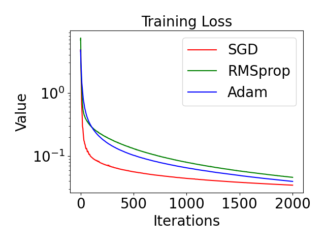
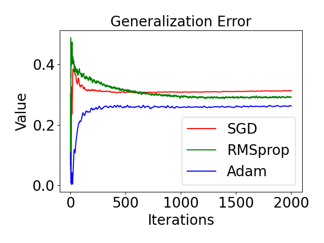
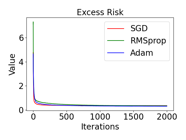
Figure 1: Results of digits dataset under cross entropy loss. From the left to right are respectively training loss, generalization error, and excess risk.

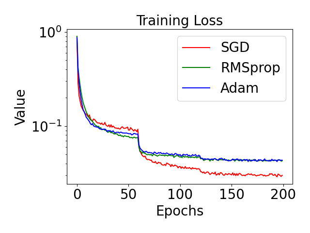
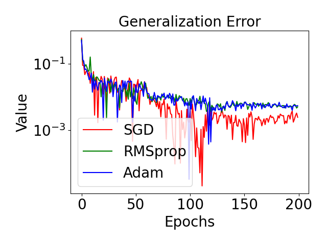
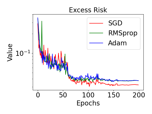
Figure 2: Results of MNIST dataset on LeNet5. From the left to right are respectively training loss, generalization error and excess risk.

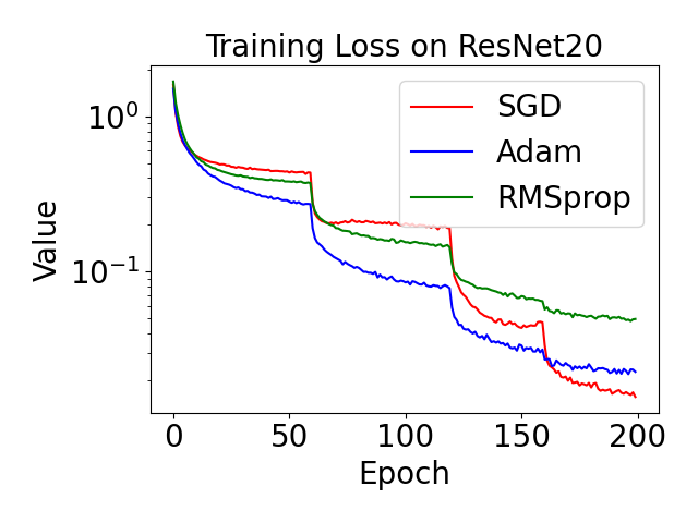
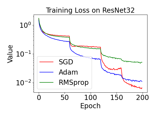
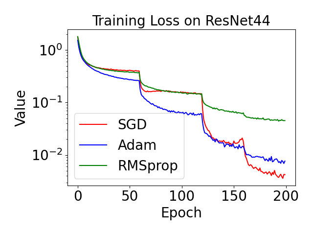
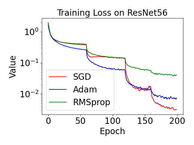
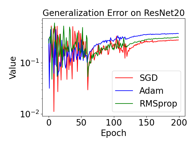
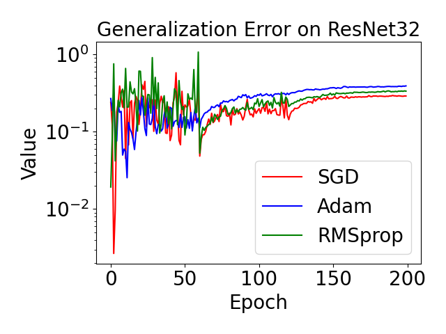
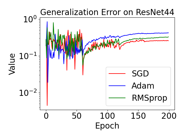
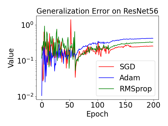
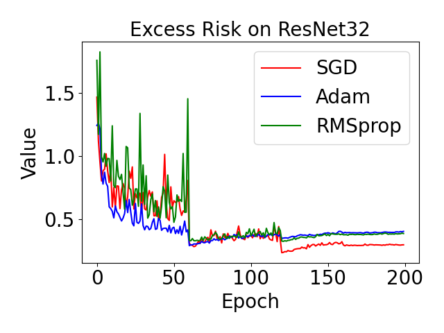
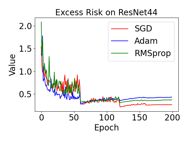
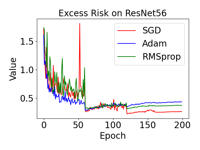
Figure 3: Results of CIFAR10 dataset on various structures of ResNet i.e., $20,32,44,56$. From the left to right are respectively training loss, generalization error and excess risk.

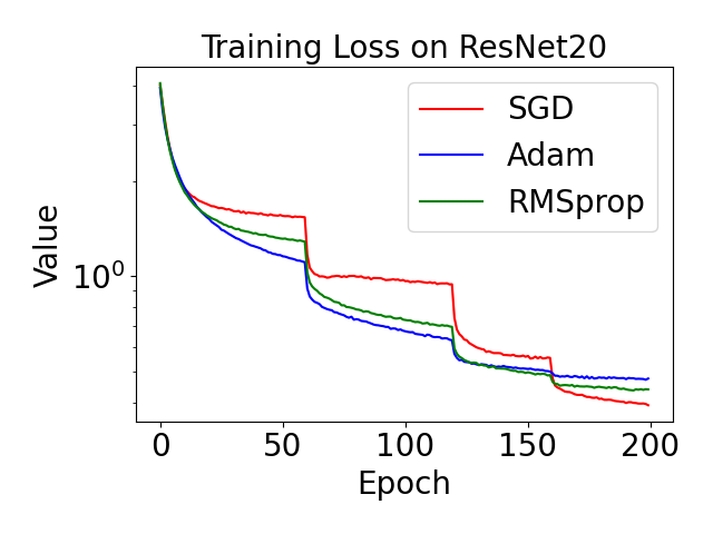
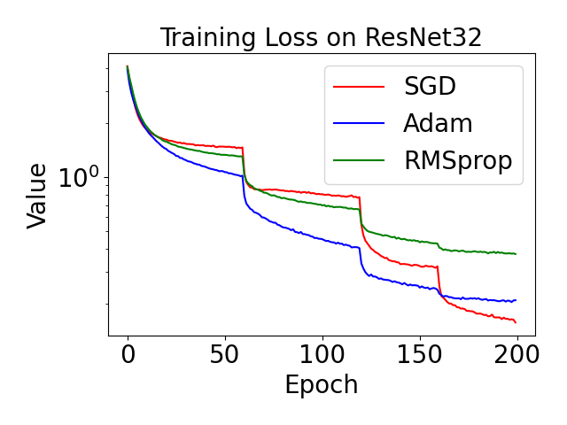
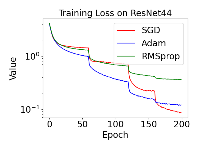
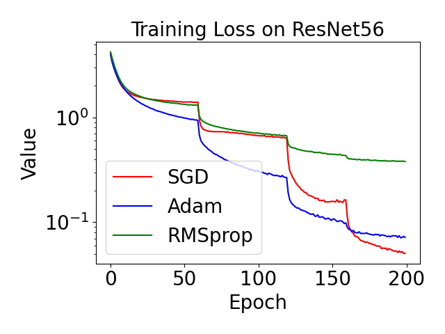
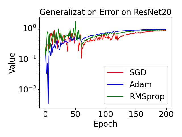
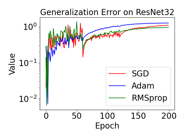
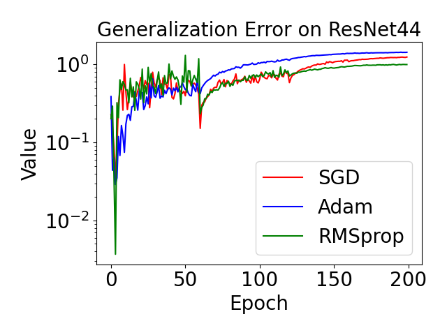
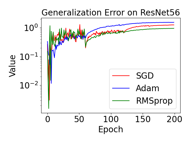
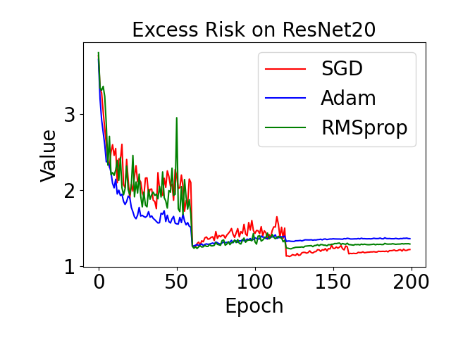
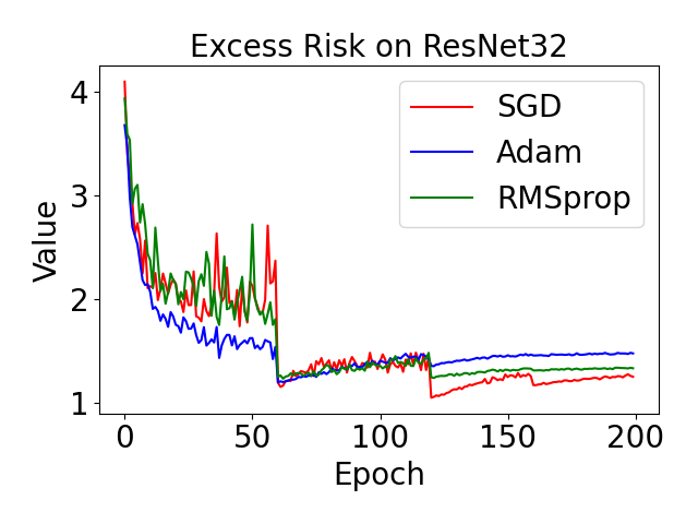
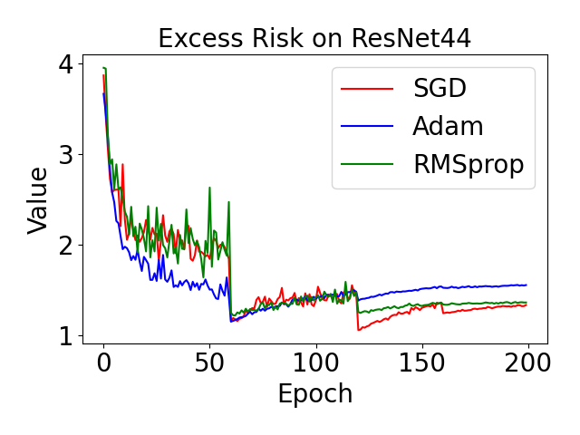
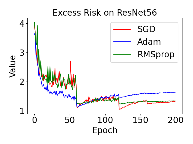
Figure 4: Results of CIFAR100 dataset on various structures of ResNet i.e., $20,32,44,56$. From the left to right are respectively training loss, generalization error and excess risk.

In this section, we empirically verify our theoretical results in this paper. The experiments are respectively conducted for convex and non-convex problems. We choose SGD (Robbins and Monro,, 1951); RMSprop (Tieleman and Hinton,, 2012), and Adam (Kingma and Ba,, 2015) as three proper algorithms which are widely used in the field of machine learning. Since we can not access the exact population risk $R(\text{\boldmath{$w$}}_{t})$ as well as $\inf_{\text{\boldmath{$w$}}}R(\text{\boldmath{$w$}})$ during training. Hence, we use the loss on test set to represent the excess risk. Our experiments are conducted on a server with single NVIDIA V100 GPU. All the reported results are the average over five independent runs.

E.1 convex problems

We conduct the experiments on multi-class logistic regression to verify our results for convex problems. We use the dataset digits which is a set with $1800$ samples from $10$ classes. The dataset is available on package sklearn (Pedregosa et al.,, 2011).

We split $70\%$ data as the training set and the others are used as the test set. We follow the training strategy that all the experiments are conducted for 2000 steps, the learning rates are respectively $0.1$, $0.001$, and $0.001$ for SGD, RMSprop, and Adam. They are decayed with the inverse square root of update steps. The results are summarized in the Figure 1.

From the results, we see that training loss for the three proper algorithms converge close to zero, while the generalization error and excess risk converge to a constant. The observation is consistent with our theoretical conclusion in Section 3.

E.2 Non-convex problems on Neural Network

For the non-convex problem, we conduct experiments on image classification with various neural network models. Specifically, we use convolutional neural networks LeNet5 (LeCun et al.,, 1998) and ResNet (He et al.,, 2016). The two structures are widely used in the image classification tasks, and they are leveraged to verify our conclusions for non-convex problems with model parameters in the same order of $n$ and much larger than $n$.

For both structures, we follow the classical training strategy. All the experiments are conducted for $200$ epochs with cross entropy loss. The learning rates are set to be $0.1,0.002,0.001$ respectively for SGD, RMSprop, and Adam. More ever, the learning rates are decayed by a factor $0.2$ at epoch $60,120,160$. We use a uniform batch size $128$ and weight decay $0.0005$.

E.2.1 Model Parameters in the Same Order of Training Samples

Data.

The dataset is MNIST (LeCun et al.,, 1998) which contain binary images of handwritten digits with $50000$ training samples and $10000$ test samples.

Model.

The model is LeNet5 which is a five layer convolutional neural network with nearly $60,000$ number of parameters.

Main Results.

The results are summarized in Figure 2. Our code is based on https://github.com/activatedgeek/LeNet-5. From the results, we see that the training loss monotonically decreases with the update steps, while both the generalization error and excess risk tend to converge to some constant. This is consistent with our theoretical results in Section 4.2 when $d$ is in the same order of $n$.

E.3 Model Parameters Larger than the Order of Training Samples

Data.

The datasets are CIFAR10 and CIFAR100 (Krizhevsky and Hinton,, 2009), which are two benchmark datasets of colorful images both with $50000$ training samples, $10000$ testing samples but from $10$ and $100$ object classes respectively.

Model.

The model we used is ResNet in various depths i.e., $20,32,44,56$. The four structures respectively have nearly $0.27$, $0.46$, $0.66$, and $0.85$ millions of parameters.

Main Results.

The experimental results for CIFAR10 and CIFAR100 are respectively in Figure 3 and 4. Our code is based on https://github.com/kuangliu/pytorch-cifar. The results show the optimization error, generalization error, and excess risk exhibit similar trends as the results on MNIST dataset. Thus, although our bounds in Section 4 are non-vacuous when $d$ is in the same order of $n$. The empirical verification on the over-parameterized neural network indicates that our results potentially can be applied to the regime of $d\gg n$.

Appendix F Examples

In this Section, we present three examples satisfies our assumptions imposed in this paper. Let us start with a linear regression problem for convex optimization.

Example 1 (Linear Regression).

Let $\boldsymbol{z}=(\boldsymbol{x},y)$, $y=\boldsymbol{x}^{\top}\text{\boldmath{$w$}}^{*}+\epsilon$ for independent noise $\epsilon$, and $f(\text{\boldmath{$w$}},\boldsymbol{z})=(y-\text{\boldmath{$w$}}^{\top}\boldsymbol{x})^{2}$.

For any $\boldsymbol{z}$, the quadratic loss $f(\text{\boldmath{$w$}},\boldsymbol{z})$ is convex, and satisfies our smoothness condition Assumption 1. Obviously, when the Hessian of population risk $E[\boldsymbol{x}\boldsymbol{x}^{\top}]$ is positively definite, the population risk is local (global) strongly convex, thus Assumptions 1, 2, and 3 are satisfied. However, for any instantaneous loss $f(\text{\boldmath{$w$}},z)$ has Hessian of $\boldsymbol{x}\boldsymbol{x}^{\top}$ which means $f(\text{\boldmath{$w$}},\boldsymbol{z})$ is not necessarily strongly convex with respect to $w$ for any $\boldsymbol{z}$. Thus, we can only treat it as a convex loss function when applying the technique in (Hardt et al.,, 2016), and get the excess risk bound of order $O(\sqrt{1/n})$. However, the empirical minimizer has a excess risk of order $O(1/n)$ which matches our result. By the way, the technique in (Zhang et al., 2017a, ) also can be applied here, while they require the number of data is sufficiently large, while we do not have such requirement.

The above example has a globally strongly convex population risk, let us consider the following example with locally but not globally strongly convex population risk.

Example 2 (Robust Regression).

Let $\boldsymbol{z}=(\boldsymbol{x},y)$, $y=\boldsymbol{x}^{\top}\text{\boldmath{$w$}}^{*}+\epsilon$ for independent noise $\epsilon$, and $f(\text{\boldmath{$w$}},\boldsymbol{z})=\phi(y-\text{\boldmath{$w$}}^{\top}\boldsymbol{x})$, with

$$\small\phi(u)=\begin{cases}u^{2}-\frac{1}{3}u^{3}\qquad&0\leq u\leq 1,\\ u^{2}+\frac{1}{3}u^{3}\qquad&0\leq u\leq 1,\\ |u|&|u|\geq 1.\end{cases}$$ (164)

By computing the gradient and Hessian, one can verify that for any $\boldsymbol{z}$, our robust regression loss $f(\text{\boldmath{$w$}},\boldsymbol{z})$ is convex, and satisfies our smoothness condition Assumption 1. Again, when the matrix $E[\boldsymbol{x}\boldsymbol{x}^{\top}]$ is positively definite, the population risk of this example is locally but not globally strongly convex. Then the example satisfies our Assumption 1-3. One can also show that the empirical risk minimizer has the generalization bound of order $\mathcal{O}(1/n)$ when $\mathbb{E}[\epsilon^{2}]$ is small enough. The error also matches our generalization bound in Theorem 2.

Finally, we consider an example of non-convex loss that satisfies our imposed Assumptions 1 and 4.

Example 3.

Let $\boldsymbol{z}_{i}$ be mixture Gaussian data such that $\boldsymbol{z}_{i}\sim\frac{1}{2}\mathcal{N}(\text{\boldmath{$w$}}_{1}^{*},\boldsymbol{I})+\frac{1}{2}\mathcal{N}(\text{\boldmath{$w$}}_{2}^{*},\boldsymbol{I})=p_{\text{\boldmath{$w$}}^{*}}(\cdot)$. The maximizing likelihood loss is $f(\text{\boldmath{$w$}},\boldsymbol{z})=-\log{p_{\text{\boldmath{$w$}}}(\boldsymbol{z})}$.

By checking the gradient and Hessian, the loss function $f(\text{\boldmath{$w$}},\boldsymbol{z})$ satisfies smoothness Assumption 1. The population risk $R(\text{\boldmath{$w$}})=-E_{\boldsymbol{z}\sim p_{\text{\boldmath{$w$}}^{*}}}[\log{p_{\text{\boldmath{$w$}}}(\boldsymbol{z})}]$, which has two global minima $(\text{\boldmath{$w$}}_{1}^{*},\text{\boldmath{$w$}}_{2}^{*}),(\text{\boldmath{$w$}}_{2}^{*},\text{\boldmath{$w$}}_{1}^{*})$, and a saddle point $((\text{\boldmath{$w$}}_{1}^{*}+\text{\boldmath{$w$}}_{2}^{*})/2,(\text{\boldmath{$w$}}_{1}^{*}+\text{\boldmath{$w$}}_{2}^{*})/2)$. Thus, this problem violates the PL-inequality which says that every local minima are global minima. However, by Lemma 16 in (Mei et al.,, 2018), we can compute the Hessian to check that the two population global minima are all strict local minima, while the saddle point is strict saddle point. Thus, the example satisfies our Assumptions 1 and 4.

References

- Allen-Zhu et al., (2019) Allen-Zhu, Z., Li, Y., and Song, Z. (2019). A convergence theory for deep learning via over-parameterization. In International Conference on Machine Learning.
- Arora et al., (2018) Arora, S., Li, Z., and Lyu, K. (2018). Theoretical analysis of auto rate-tuning by batch normalization. In International Conference on Learning Representations.
- Bartlett and Mendelson, (2002) Bartlett, P. L. and Mendelson, S. (2002). Rademacher and gaussian complexities: Risk bounds and structural results. Journal of Machine Learning Research, 3(11):463–482.
- Bartlett et al., (2021) Bartlett, P. L., Montanari, A., and Rakhlin, A. (2021). Deep learning: a statistical viewpoint. Preprint arXiv:2103.09177.
- Bian et al., (2015) Bian, W., Chen, X., and Ye, Y. (2015). Complexity analysis of interior point algorithms for non-lipschitz and nonconvex minimization. Mathematical Programming, 149(1-2):301–327.
- Bickel et al., (2009) Bickel, P. J., Ritov, Y., Tsybakov, A. B., et al. (2009). Simultaneous analysis of lasso and dantzig selector. The Annals of Statistics, 37(4):1705–1732.
- Blumer et al., (1989) Blumer, A., Ehrenfeucht, A., Haussler, D., and Warmuth, M. K. (1989). Learnability and the vapnik-chervonenkis dimension. Journal of the ACM, 36(4):929–965.
- Bottou et al., (2018) Bottou, L., Curtis, F. E., and Nocedal, J. (2018). Optimization methods for large-scale machine learning. SIAM Review, 60(2):223–311.
- Bousquet and Elisseeff, (2002) Bousquet, O. and Elisseeff, A. (2002). Stability and generalization. Journal of Machine Learning Research, 2(3):499–526.
- Bousquet et al., (2020) Bousquet, O., Klochkov, Y., and Zhivotovskiy, N. (2020). Sharper bounds for uniformly stable algorithms. In Conference on Learning Theory.
- Bu et al., (2020) Bu, Y., Zou, S., and Veeravalli, V. V. (2020). Tightening mutual information-based bounds on generalization error. IEEE Journal on Selected Areas in Information Theory, 1(1):121–130.
- Bubeck, (2014) Bubeck, S. (2014). Convex optimization: Algorithms and complexity. Preprint arXiv:1405.4980.
- Cartis et al., (2018) Cartis, C., Gould, N. I., and Toint, P. L. (2018). Second-order optimality and beyond: Characterization and evaluation complexity in convexly constrained nonlinear optimization. Foundations of Computational Mathematics, 18(5):1073–1107.
- Charles and Papailiopoulos, (2018) Charles, Z. and Papailiopoulos, D. (2018). Stability and generalization of learning algorithms that converge to global optima. In International Conference on Machine Learning.
- (15) Chen, X., Liu, S., Sun, R., and Hong, M. (2018a). On the convergence of a class of adam-type algorithms for non-convex optimization. In International Conference on Learning Representations.
- (16) Chen, Y., Jin, C., and Yu, B. (2018b). Stability and convergence trade-off of iterative optimization algorithms. Preprint arXiv:1804.01619.
- Cherkassky et al., (1999) Cherkassky, V., Shao, X., Mulier, F. M., and Vapnik, V. N. (1999). Model complexity control for regression using VC generalization bounds. IEEE Transactions on Neural Networks, 10(5):1075–1089.
- Cynthia et al., (2015) Cynthia, D., Vitaly, F., Moritz, H., Toniann, P., Omer, R., and Aaron, R. (2015). A new analysis of differential privacy’s generalization guarantees. In ACM Symposium on Theory of Computing.
- Daneshmand et al., (2018) Daneshmand, H., Kohler, J., Lucchi, A., and Hofmann, T. (2018). Escaping saddles with stochastic gradients. In International Conference on Machine Learning.
- Deng et al., (2020) Deng, Z., He, H., and Su, W. (2020). Toward better generalization bounds with locally elastic stability. Preprint arXiv:2010.13988.
- Du et al., (2019) Du, S., Lee, J. D., Li, H., Wang, L., and Zhai, X. (2019). Gradient descent finds global minima of deep neural networks. In International Conference on Machine Learning.
- Fan et al., (2017) Fan, J., Li, Q., and Wang, Y. (2017). Estimation of high dimensional mean regression in the absence of symmetry and light tail assumptions. Journal of the Royal Statistical Society. Series B, Statistical methodology, 79(1):247.
- Fang et al., (2018) Fang, C., Li, C. J., Lin, Z., and Zhang, T. (2018). Spider: Near-optimal non-convex optimization via stochastic path-integrated differential estimator. In Advances in Neural Information Processing Systems.
- Fang et al., (2019) Fang, C., Lin, Z., and Zhang, T. (2019). Sharp analysis for nonconvex sgd escaping from saddle points. In Conference on Learning Theory.
- Feldman, (2016) Feldman, V. (2016). Generalization of erm in stochastic convex optimization: The dimension strikes back. In Advances in Neural Information Processing Systems.
- Feldman and Vondrak, (2019) Feldman, V. and Vondrak, J. (2019). High probability generalization bounds for uniformly stable algorithms with nearly optimal rate. In Conference on Learning Theory.
- Ge et al., (2015) Ge, R., Huang, F., Jin, C., and Yuan, Y. (2015). Escaping from saddle points—online stochastic gradient for tensor decomposition. In Conference on Learning Theory.
- Ge et al., (2016) Ge, R., Lee, J. D., and Ma, T. (2016). Matrix completion has no spurious local minimum. In Advances in Neural Information Processing Systems.
- Ghadimi and Lan, (2013) Ghadimi, S. and Lan, G. (2013). Stochastic first-and zeroth-order methods for nonconvex stochastic programming. SIAM Journal on Optimization, 23(4):2341–2368.
- Gonen and Shalev-Shwartz, (2017) Gonen, A. and Shalev-Shwartz, S. (2017). Fast rates for empirical risk minimization of strict saddle problems. In Conference on Learning Theory.
- Guyon et al., (1993) Guyon, I., Boser, B. E., and Vapnik, V. (1993). Automatic capacity tuning of very large vc-dimension classifiers. In Advances in Neural Information Processing Systems.
- Hardt et al., (2016) Hardt, M., Recht, B., and Singer, Y. (2016). Train faster, generalize better: Stability of stochastic gradient descent. In International Conference on Machine Learning.
- He et al., (2016) He, K., Zhang, X., Ren, S., and Sun, J. (2016). Deep residual learning for image recognition. In Conference on Computer Vision and Pattern Recognition.
- Hoffer et al., (2017) Hoffer, E., Hubara, I., and Soudry, D. (2017). Train longer, generalize better: closing the generalization gap in large batch training of neural networks. In Advances in Neural Information Processing Systems.
- Javanmard and Montanari, (2014) Javanmard, A. and Montanari, A. (2014). Confidence intervals and hypothesis testing for high-dimensional regression. Journal of Machine Learning Research, 15(1):2869–2909.
- Javanmard et al., (2018) Javanmard, A., Montanari, A., et al. (2018). Debiasing the lasso: Optimal sample size for gaussian designs. The Annals of Statistics, 46(6A):2593–2622.
- Jin et al., (2017) Jin, C., Ge, R., Netrapalli, P., Kakade, S. M., and Jordan, M. I. (2017). How to escape saddle points efficiently. In International Conference on Machine Learning.
- Jin et al., (2018) Jin, C., Liu, L. T., Ge, R., and Jordan, M. I. (2018). On the local minima of the empirical risk. In Advances in Neural Information Processing Systems.
- Jin et al., (2019) Jin, C., Netrapalli, P., Ge, R., Kakade, S. M., and Jordan, M. I. (2019). Stochastic gradient descent escapes saddle points efficiently. Preprint arXiv:1902.04811.
- Johnson and Zhang, (2013) Johnson, R. and Zhang, T. (2013). Accelerating stochastic gradient descent using predictive variance reduction. In Advances in Neural Information Processing Systems.
- Jung and Ligett, (2020) Jung, C. and Ligett, K. (2020). A new analysis of differential privacy’s generalization guarantees. In Innovations in Theoretical Computer Science.
- Karimi et al., (2016) Karimi, H., Nutini, J., and Schmidt, M. (2016). Linear convergence of gradient and proximal-gradient methods under the polyak-łojasiewicz condition. In European Conference on Machine Learning and Knowledge Discovery in Databases.
- Kawaguchi, (2016) Kawaguchi, K. (2016). Deep learning without poor local minima. In Advances in Neural Information Processing Systems.
- Kingma and Ba, (2015) Kingma, D. P. and Ba, J. (2015). Adam: A method for stochastic optimization. In International Conference on Learning Representations.
- Krizhevsky and Hinton, (2009) Krizhevsky, A. and Hinton, G. (2009). Learning multiple layers of features from tiny images.
- LeCun et al., (1998) LeCun, Y., Bottou, L., Bengio, Y., and Haffner, P. (1998). Gradient-based learning applied to document recognition. Proceedings of the IEEE, 86(11):2278–2324.
- Li and Liu, (2022) Li, S. and Liu, Y. (2022). High probability guarantees for nonconvex stochastic gradient descent with heavy tails. In International Conference on Machine Learning.
- Liu et al., (2022) Liu, C., Zhu, L., and Belkin, M. (2022). Loss landscapes and optimization in over-parameterized non-linear systems and neural networks. Applied and Computational Harmonic Analysis.
- Mei et al., (2018) Mei, S., Bai, Y., and Montanari, A. (2018). The landscape of empirical risk for nonconvex losses. The Annals of Statistics, 46(6A):2747–2774.
- Meng et al., (2017) Meng, Q., Wang, Y., Chen, W., Wang, T., Ma, Z.-M., and Liu, T.-Y. (2017). Generalization error bounds for optimization algorithms via stability. In Association for the Advancement of Artificial Intelligence.
- Mohri and Rostamizadeh, (2009) Mohri, M. and Rostamizadeh, A. (2009). Rademacher complexity bounds for non-iid processes. In Advances in Neural Information Processing Systems.
- Mokhtari et al., (2018) Mokhtari, A., Ozdaglar, A., and Jadbabaie, A. (2018). Escaping saddle points in constrained optimization. In Advances in Neural Information Processing Systems.
- Negrea et al., (2019) Negrea, J., Haghifam, M., Dziugaite, G. K., Khisti, A., and Roy, D. M. (2019). Information-theoretic generalization bounds for sgld via data-dependent estimates. Advances in Neural Information Processing Systems.
- Neu et al., (2021) Neu, G., Dziugaite, G. K., Haghifam, M., and Roy, D. M. (2021). Information-theoretic generalization bounds for stochastic gradient descent. In Conference on Learning Theory.
- Neyshabur et al., (2018) Neyshabur, B., Li, Z., Bhojanapalli, S., LeCun, Y., and Srebro, N. (2018). The role of over-parametrization in generalization of neural networks. In International Conference on Learning Representations.
- (56) Nguyen, L. M., Liu, J., Scheinberg, K., and Takáč, M. (2017a). Sarah: A novel method for machine learning problems using stochastic recursive gradient. In International Conference on Machine Learning.
- (57) Nguyen, L. M., Liu, J., Scheinberg, K., and Takáč, M. (2017b). Stochastic recursive gradient algorithm for nonconvex optimization. Preprint arXiv:1705.07261.
- Nocedal and Wright, (2006) Nocedal, J. and Wright, S. (2006). Numerical optimization. Springer Science & Business Media.
- Opper, (1994) Opper, M. (1994). Learning and generalization in a two-layer neural network: The role of the vapnik-chervonvenkis dimension. Physical Review Letters, 72(13):2113.
- Pedregosa et al., (2011) Pedregosa, F., Varoquaux, G., Gramfort, A., Michel, V., Thirion, B., Grisel, O., Blondel, M., Prettenhofer, P., Weiss, R., Dubourg, V., et al. (2011). Scikit-learn: Machine learning in Python. Journal of Machine Learning Research, 12:2825–2830.
- Robbins and Monro, (1951) Robbins, H. and Monro, S. (1951). A stochastic approximation method. The Annals of Mathematical Statistics, pages 400–407.
- Roux et al., (2012) Roux, N. L., Schmidt, M., and Bach, F. (2012). A stochastic gradient method with an exponential convergence _rate for finite training sets. In Advances in Neural Information Processing Systems.
- Shalev-Shwartz et al., (2009) Shalev-Shwartz, S., Shamir, O., Srebro, N., and Sridharan, K. (2009). Stochastic convex optimization. In Conference on Learning Theory.
- Shamir and Zhang, (2013) Shamir, O. and Zhang, T. (2013). Stochastic gradient descent for non-smooth optimization: Convergence results and optimal averaging schemes. In International Conference on Machine Learning.
- Shawe-Taylor and Williamson, (1999) Shawe-Taylor, J. and Williamson, R. C. (1999). Generalization performance of classifiers in terms of observed covering numbers. In European Conference on Computational Learning Theory.
- Sinha et al., (2018) Sinha, A., Namkoong, H., and Duchi, J. (2018). Certifying some distributional robustness with principled adversarial training. In International Conference on Learning Representations.
- Steinke and Zakynthinou, (2020) Steinke, T. and Zakynthinou, L. (2020). Reasoning about generalization via conditional mutual information. In Conference on Learning Theory.
- Tieleman and Hinton, (2012) Tieleman, T. and Hinton, G. (2012). Lecture 6.5-rmsprop: Divide the gradient by a running average of its recent magnitude. COURSERA: Neural networks for machine learning, 4(2):26–31.
- Vapnik, (1999) Vapnik, V. (1999). The nature of statistical learning theory. Springer science & business media.
- Vaswani et al., (2017) Vaswani, A., Shazeer, N., Parmar, N., Uszkoreit, J., Jones, L., Gomez, A. N., Kaiser, Ł., and Polosukhin, I. (2017). Attention is all you need. In Advances in Neural Information Processing Systems.
- Vershynin, (2018) Vershynin, R. (2018). High-dimensional probability: An introduction with applications in data science. Cambridge Series in Statistical and Probabilistic Mathematics. Cambridge University Press.
- Wainwright, (2019) Wainwright, M. J. (2019). High-dimensional statistics: A non-asymptotic viewpoint. Cambridge Series in Statistical and Probabilistic Mathematics. Cambridge University Press.
- Williamson et al., (2001) Williamson, R. C., Smola, A. J., and Scholkopf, B. (2001). Generalization performance of regularization networks and support vector machines via entropy numbers of compact operators. IEEE Transactions on Information Theory, 47(6):2516–2532.
- Xu and Raginsky, (2017) Xu, A. and Raginsky, M. (2017). Information-theoretic analysis of generalization capability of learning algorithms. In Advances in Neural Information Processing Systems.
- Xu and Mannor, (2012) Xu, H. and Mannor, S. (2012). Robustness and generalization. Machine learning, 86(3):391–423.
- Xu et al., (2018) Xu, Y., Jin, R., and Yang, T. (2018). First-order stochastic algorithms for escaping from saddle points in almost linear time. In Advances in Neural Information Processing Systems.
- (77) Yi, M., Hou, L., Sun, J., Shang, L., Jiang, X., Liu, Q., and Ma, Z.-M. (2021a). Improved ood generalization via adversarial training and pre-training. In International Conference on Machine Learning.
- (78) Yi, M., Meng, Q., Chen, W., and Ma, Z.-M. (2021b). Towards accelerating training of batch normalization: A manifold perspective. Preprint arXiv:2101.02916.
- Yuan et al., (2019) Yuan, Z., Yan, Y., Jin, R., and Yang, T. (2019). Stagewise training accelerates convergence of testing error over sgd. In Advances in Neural Information Processing Systems.
- Zhang, (2010) Zhang, C.-H. (2010). Nearly unbiased variable selection under minimax concave penalty. The Annals of Statistics, 38(2):894–942.
- (81) Zhang, L., Yang, T., and Jin, R. (2017a). Empirical risk minimization for stochastic convex optimization: -and -type of risk bounds. In Conference on Learning Theory.
- Zhang, (2002) Zhang, T. (2002). Covering number bounds of certain regularized linear function classes. Journal of Machine Learning Research, 2(3):527–550.
- Zhang et al., (2013) Zhang, Y., Duchi, J. C., and Wainwright, M. J. (2013). Communication-efficient algorithms for statistical optimization. The Journal of Machine Learning Research, 14(1):3321–3363.
- (84) Zhang, Y., Liang, P., and Charikar, M. (2017b). A hitting time analysis of stochastic gradient langevin dynamics. In Conference on Learning Theory.
- Zou et al., (2020) Zou, D., Cao, Y., Zhou, D., and Gu, Q. (2020). Gradient descent optimizes over-parameterized deep relu networks. Machine Learning, 109(3):467–492.