Improving phase estimation using the number-conserving operations

Abstract

We propose a theoretical scheme to improve the resolution and precision of phase measurement with parity detection in the Mach-Zehnder interferometer by using a nonclassical input state which is generated by applying a number-conserving generalized superposition of products (GSP) operation, $\left(saa^{\dagger}+ta^{\dagger}a\right)^{m}$ with $s^{2}+t^{2}=1$, on two-mode squeezed vacuum (TMSV) state. The nonclassical properties of the proposed GSP-TMSV are investigated via average photon number (APN), anti-bunching effect, and degrees of two-mode squeezing. Particularly, our results show that both higher-order $m$ GSP operation and smaller parameter $s$ can increase the total APN, which leads to the improvement of quantum Fisher information. In addition, we also compare the phase measurement precision with and without photon losses between our scheme and the previous photon subtraction/addition schemes. It is found that our scheme, especially for the case of $s=0$, has the best performance via the enhanced phase resolution and sensitivity when comparing to those previous schemes even in the presence of photon losses. Interestingly, without losses, the standard quantum-noise limit (SQL) can always be surpassed in our our scheme and the Heisenberg limit (HL) can be even achieved when $s=0.5,1$ with small total APNs. However, in the presence of photon losses, the HL cannot be beaten, but the SQL can still be overcome particularly in the large total APN regimes. Our results here can find important applications in quantum metrology.

PACS: 03.67.-a, 05.30.-d, 42.50,Dv, 03.65.Wj

I Introduction

The ultimate aim of quantum metrology is to achieve a higher precision and sensitivity of the phase estimation using (non)classical field of light as the input of optical interferometers 1 ; 2 ; 3 ; 4 . Among them, the Mach-Zehnder interferometer (MZI) is one of the most practical interferometers, and its phase sensitivity is limited by the standard quantum-noise limit (SQL) $\Delta\varphi=1/\sqrt{N}$ ($N$ is the average number of photons inside the interferometer), together with solely classical resources as the input of the MZI 5 . In order to go beyond this limit, both the nonclassical states 6 ; 7 and the entangled states 2 ; 8 ; 9 are applied to quantum metrology, which results in the reduction of the phase uncertainty, thereby reaching the Heisenberg limit (HL) $\Delta\varphi=1/N$ 10 . For instance, Dowling et al. 2 pointed out that the so-called N00N states in quantum optical interferometry can achieve the HL. Unfortunately, these states are extremely sensitive to photon losses 9 ; 10 ; 11 . To solve this problem, Anisimov et al. 8 theoretically studied that using the two-mode squeezed vacuum state (TMSV) as the input of the MZI with parity detection scheme can reach the so-called sub-Heisenberg limit with small total average photon numbers (APN). However, restricted by current experimental techniques, it is still difficult to generate strongly entangled TMSV in which its maximum obtainable degree is about $r=1.15$ $(\overline{n}=\sinh^{2}r\approx 2)$ 14 . Thus, how to prepare highly non-classical and strongly entangled quantum states has become one of the most important topics in quantum information and quantum metrology.

For this purpose, the usage of non-Gaussian operations 15 ; 16 ; 17 ; 18 ; 19 ; 20 ; 21 ; 22 ; 23 ; 24 is a feasible method, e.g., photon subtraction (PS) 15 , photon addition (PA) 18 ; 19 ; 20 ; 21 ; 22 , and their superposition 23 ; 24 , which also plays an vital role in quantum illumination 25 ; 26 , quantum cryptography 27 ; 28 ; 29 ; 30 ; 31 and quantum teleportation 32 ; 33 ; 34 . For instance, Agarwal and Tara proposed that the classical coherent states can be transformed into highly nonclassical quantum states by the PA operation 18 and this PA operation can be experimentally implemented which was proposed by Zavatta 19 . In addition, highly nonclassicality has been shown for the PA- (or PS-) squeezed states 35 ; 36 . Based on the facts mentioned above, Gerry et al. 6 first proposed to use the PS-TMSV (simultaneously subtracting the same number of photons from the TMSV ) as the input of the MZI, and showed that the phase measurement uncertainty of the PS-TMSV scheme is smaller than that of the usual TMSV for the same squeezing parameters. Then, Ouyang et al. 22 used the PA-TMSV as the input state of the MZI, and showed that it has better performance in terms of phase sensitivity for small phase shift when compared with both the PS-TMSV and the usual TMSV. In addition to the aforementioned typical non-Gaussian operations, here we suggest to use a new type of non-Gaussian states as the input of the MZI in an attempt to further enhance the resolution and sensitivity of the phase estimation. The non-Gaussian states we consider here are the output states by applying the number-conserving generalized superposition of products (GSP) operation $\left(saa^{\dagger}+ta^{\dagger}a\right)$ with $s^{2}+t^{2}=1$, to the TMSV. It is interesting to notice that the PA-then-PS ($aa^{\dagger}$) and the PS-then-PA ($a^{\dagger}a$) as well as their superposition can be considered as three special cases in our scheme. In particular, the first two have been used to improve entanglement and fidelity of quantum teleportation, but none of them are used to improve phase measurement accuracy. Not only can this GSP operation be implemented experimentally, proposed by Kim 37 , but also the GSP operation on the TMSV is able to generate a strongly entangled non-Gaussian state as well 38 ; 39 .

In order to extract quantum phase information more effectively, three types of detection schemes are usually used, including intensity detection 40 ; 41 , homodyne detection 42 and parity detection 43 ; 44 . It should be noted that not all detection schemes can employ the full potential of nonclassical states to achieve the superresolution and supersensitivity. In particular, as referred to Ref. 45 , the intensity detection is more suitable for optical interferometers with coherent light as input, but it is not applicable to the TMSV. In contrast, the parity detection can be used in the quantum metrology with the TMSV to achieve the superresolution and even sub-Heisenberg limit sensitivity 8 ; 46 ; 47 . Thus, in this paper, we take advantage of parity detection to extract phase information and study the phase resolution and sensitivity of the MZI by using the GSP-TMSV as input. The numerical simulation results show that our scheme, especially for the case of the PS-then-PA TMSV ($s=0$), is always superior to the original TMSV scheme in terms of the quantum Fisher information (QFI) and the phase resolution and sensitivity. Dramatically, the SQL can be always surpassed in our scheme and the HL can even be beaten for the cases when $s=0.5,1$ in the regime of small total APN. Furthermore, since the interaction with the environment is inevitable, we also investigate the effects of GSP operations against the photon losses placed in front of parity detection (denoted as an external loss) and between the phase shifter and the second beam splitter (BS) (denoted as an internal loss) from a practical point of view. Our results show that in the presence of photon losses the phase sensitivity with the GSP-TMSV, especially for the case of $s=0$, can still be better than that with both the TMSV and the PA(PS)-TMSV under the same accessible parameters. Interestingly, we also find that the effects of the external losses on phase uncertainty are more serious than the internal-loss cases.

The structure of this paper is organized as follows: In Sec. II, we briefly outline the preparation of the GSP-TMSV state, and then present its nonclassicality according to APN, antibunching effect and two-mode squeezing property. In Sec. III, we show the application of the GSP-TMSV in the MZI and mainly focus on its QFI behavior. The resolution and sensitivity of phase estimation with parity detection are further discussed in Sec. IV. In Sec. V, we mainly pay attention to the effects of photon losses, involving external and internal losses, on the resolution and sensitivity. Finally, the main results are summarized in Sec. VI.

II The generation of the GSP-TMSV and nonclassical properties

In this section, we first introduce the GSP-TMSV in theory, and then show its nonclassicality by means of APN, anti-bunching effect and two-mode squeezing property.

II.1 The generation of the GSP-TMSV

Figure 1: (Color online) Schematic diagram of a balanced MZI for the detection of the phase shift (Violet) when the GSP-TMSV state is sent to the first BS (Green), and the photon-number parity measurements are performed on the output $b$ mode.

In recent years, it has been demonstrated that both the PS-TMSV and the PA-TMSV as the inputs of the MZI can improve the phase sensitivity effectively 6 ; 22 , since these nonGaussian states have the advantages over the Gaussian states in terms of the nonclassicality and the entanglement degree. In this section, we introduce a new kind of non-Gaussian state, the GSP-TMSV, which can be prepared by acting two GSP operations on the TMSV, as pictured in Fig.1 (orange box). As referred to 38 ; 39 , this GSP operation can be seen as an equivalent operator

$$\hat{O}=\left(s_{1}aa^{\dagger}+t_{1}a^{\dagger}a\right)^{m}\left(s_{2}bb^{\dagger}+t_{2}b^{\dagger}b\right)^{n},$$ (1)

where $s_{i}^{2}+t_{i}^{2}=1\ (i=1,2)$ and both $a$ $\left(a^{\dagger}\right)$ and $b$ $\left(b^{\dagger}\right)$ are annihilation (creation) operators for modes $a$ and $b$, respectively. Note that $\left(m,n\right)$ represent $m$-order operation of $s_{1}aa^{\dagger}+t_{1}a^{\dagger}a$ on mode $a$ and $n$-order operation of $s_{2}bb^{\dagger}+t_{2}b^{\dagger}b$ on mode $b$. Thus, the GSP-TMSV can be given by

$$\left|\psi\right\rangle_{ab} = \frac{\hat{O}S_{2}\left(z\right)}{\sqrt{P_{d}}}\left|00\right\rangle$$ (2)

$$= \frac{\Re u}{\sqrt{P_{d}}}\exp\left(va^{\dagger}b^{\dagger}\right)\left|00\right\rangle,$$

with

$$\Re = \frac{\partial^{m+n}}{\partial\tau_{1}^{m}\partial\tau_{2}^{n}}\left\{\cdot\right\}|_{\tau_{1}=\tau_{2}=0},$$

$$u = \sqrt{1-z^{2}}\exp\left(s_{1}\tau_{1}+s_{2}\tau_{2}\right),$$

$$v = z\exp\left(s_{1}\tau_{1}+t_{1}\tau_{1}+s_{2}\tau_{2}+t_{2}\tau_{2}\right),$$ (3)

where $S_{2}\left(z\right)=\exp[\left(a^{\dagger}b^{\dagger}-ab\right)$arctanh $z]$ is the two-mode squeezing operator with a squeezing parameter $z$ and $P_{d}$ is a normalization coefficient which can be calculated as

$$P_{d}=\widetilde{\Re}\frac{uu_{1}}{1-vv_{1}},$$ (4)

with

$$\widetilde{\Re} = \frac{\partial^{2m+2n}}{\partial\tau_{1}^{m}\partial\tau_{2}^{n}\partial\tau_{3}^{m}\partial\tau_{4}^{n}}\left\{\cdot\right\}_{|\tau_{1}=\tau_{2}=\tau_{3}=\tau_{4}=0},$$

$$u_{1} = \sqrt{1-z^{2}}\exp\left(s_{1}\tau_{3}+s_{2}\tau_{4}\right),$$

$$v_{1} = z\exp\left(s_{1}\tau_{3}+t_{1}\tau_{3}+s_{2}\tau_{4}+t_{2}\tau_{4}\right).$$ (5)

It should be emphasized that for simplicity, all the following simulations are based on the assumption of $s_{1}=s_{2}=s,t_{1}=t_{2}=t$. In particular, when $s=0,0.5$ and $1$, from Eqs. (1) and (2), one can obtain the PS-then-PA TMSV, a general GSP-TMSV and the PA-then-PS TMSV, respectively.

For the sake of analysis in the following, here we present the expectation value of a general quantum operator, i.e.,

$$\left\langle a^{l}b^{k}a^{\dagger h}b^{\dagger g}\right\rangle=\widetilde{\Re}\widetilde{D}P_{d}^{-1}uu_{1}\Delta e^{\Delta w},$$ (6)

with

$$\widetilde{D} = \frac{\partial^{l+k+h+g}}{\partial\tau_{5}^{l}\partial\tau_{6}^{k}\partial\tau_{7}^{h}\partial\tau_{8}^{g}}\left\{\cdot\right\}|_{\tau_{5}=\tau_{6}=\tau_{7}=\tau_{8}=0},$$

$$\Delta = \left(1-vv_{1}\right)^{-1},$$

$$w = \tau_{7}\tau_{8}v_{1}+\tau_{6}\tau_{5}v+\tau_{6}\tau_{8}+\tau_{5}\tau_{7},$$ (7)

where $l,k,h$ and $g$ are integers ($\geqslant 0$), Eq. (6) can be used to calculate some expectation values, such as $\left\langle aa^{\dagger}\right\rangle,$ $\left\langle bb^{\dagger}\right\rangle,$ $\left\langle aa^{\dagger}bb^{\dagger}\right\rangle,$ $\left\langle a^{2}b^{\dagger 2}\right\rangle,$ and $\left\langle a^{\dagger 2}b^{2}\right\rangle$.

II.2 Nonclassical properties of the GSP-TMSV

As described in Refs. 6 ; 7 , the nonclassical states of optical field offer a significant improvement in the sensitivity and precision of the MZI, thereby promoting the development of quantum metrology. Before investigating how does the GSP-TMSV as the input affect the sensitivity and resolution of the MZI, let us first examine its nonclassicality in terms of APN, anti-bunching effect and two-mode squeezing property, which provide the basis for the performance improvement of the phase estimation in next section.

II.2.1 Average photon number

As one of statistical properties of the light field, the APN is an important factor for optical interferometry. In addition, as a kind of non-Gaussian operation, the PS from squeezed vacuum state can surprisingly increase the APN, by which the phase sensitivity can be improved. Here, we first pay attention to the APN and examine if it can be increased by the GSP operation or not. According to Eq. (6), the APN, say for mode $a$, can be calculated as

$$\overline{N}_{a} =\left\langle a^{\dagger}a\right\rangle=\left\langle aa^{\dagger}\right\rangle-1$$

$$=\frac{\widetilde{\Re}uu_{1}}{P_{d}}\frac{\partial^{2}}{\partial\tau_{5}\partial\tau_{7}}\Delta e^{\Delta\tau_{5}\tau_{7}}|_{\tau_{5}=\tau_{7}=0}-1.$$ (8)

For mode $b$, there is the same result, i.e., $\overline{N}_{a}=\overline{N}_{b}=N,$ which can be easily seen from Eq. (6).

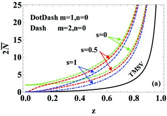
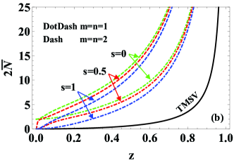
Figure 2: (Color online) Average photon number as a function of squeezing parameter $z$ for different operator parameter $s=0,0.5,1$. for (a) single-side GSP operations ($\left(m,n\right)\in\left\{\left(0,1\right),\left(0,2\right)\right\}$), (b) two-side symmetric GSP operations ($\left(m,n\right)\in\left\{\left(1,1\right),\left(2,2\right)\right\}$). Solid lines correspond to the TMSV case.

Figure 2 shows the total APN $\left(2N\right)$ before injecting into the MZI as the function of the squeezing parameter $z$ for different superposition parameters $s=0,0.5,1$. For a comparison, the APN of the TMSV is also plotted in Fig. 2, see the solid black line. From Fig. 2, it is clear that the APN of the generated states outperforms that of the TMSV in nearly all squeezing ranges for both single-side and two-side GSP operations. In addition, for a fixed superposition $s$, the APN increases as the increasing ($m,n$) and $z$. The APN with two-side symmetrical GSP ($\left(m,n\right)\in\left\{\left(1,1\right),\left(2,2\right)\right\}$) is bigger than that with single-side case ($\left(m,n\right)\in\left\{\left(0,1\right),\left(0,2\right)\right\}$) by comparing Fig. 2(a) with 2(b). On the other hand, it is interesting to notice that, for fixed $m$ and $n$, the APN decreases as the increasing $s$. In particular, in the limit $s=0,$ corresponding to the PS-then-PA case, the APN has the biggest value when other parameters are fixed. While for the case of $s=1$ corresponding to the PA-then-PS case, the APN has the lowest value when comparing with other cases for $s$. Even so, both PA-then-PS and PS-then-PA have bigger APN than the TMSV. Among these non-Gaussian operations, the PS-then-PA case presents the biggest APN.

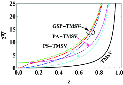
Figure 3: (Color online) As a comparison, the APN as a function of the squeezing parameter $z$. The dot-dashed lines represent our scheme for operation parameters $s=0,0.5,1$ (corresponding to green, red, and blue color line, respectively), and dashed lines represent the previous work of using the PA-TMSV (magenta color line) and the PS-TMSV (cyan color line) as inputs. Solid line corresponds to the TMSV case.

In Fig. 3, under the same parameter of $m=n=1$, we also compare about the APN $2N$ changing with $z$ for giving several non-Gaussian states, including the PA-TMSV (Magenta dashed), the PS-TMSV (cayan dashed) and the GSP-TMSV. Distinctly, the APN of the GSP-TMSV is always greater than that of the PS-TMSV for all squeezing ranges. Especially, for the PS-then-PA TMSV $\left(s=0\right)$, it presents the largest APN compared with those for the PA-TMSV and the PS-TMSV. This means that our scheme can show the advantage in terms of the total APN, which is beneficial for the improvement of QFI. We also notice that, compared with the PA-TMSV, the APN of the GSP-TMSV when $s=0.5$ $(s=1)$ is smaller at $z<0.18$ ($z<0.4$).

II.2.2 Antibunching effect of the GSP-TMSV

In this subsection, let us consider the nonclassical properties of the GSP-TMSV through the anti-bunching effect, which reflects the sub-Poisson distribution implying the existence of nonclassical states 48 . For an arbitrary two-mode system, generally, the criteria of the antibunching effect turns out to be 20 ; 49

$$R_{a,b}=\frac{\left\langle a^{\dagger 2}a^{2}\right\rangle+\left\langle b^{\dagger 2}b^{2}\right\rangle}{2\left\langle a^{\dagger}ab^{\dagger}b\right\rangle}-1.$$ (9)

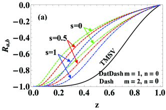
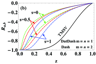
Figure 4: (Color online) The antibunching effect $R_{a,b}$ as a function of squeezing parameter $z$ for different operator parameter $s=0,0.5,1$. for (a) the single-side GSP operations ($\left(m,n\right)\in\left\{\left(0,1\right),\left(0,2\right)\right\}$), (b) the two-side symmetric GSP operations ($\left(m,n\right)\in\left\{\left(1,1\right),\left(2,2\right)\right\}$). Solid lines correspond to the TMSV case.

According to Eq. (6), we can obtain the explicit expression of anti-bunching effect $R_{a,b}$ in theory. In principle, the condition of $R_{a,b}<0$ corresponds to the existence of the antibunching effect, which means that this quantum state has the nonclassicality. To clearly see this point, in Fig. 4, we show the antibunching effect $R_{a,b}$ as the function of squeezing parameter $z$ for different several superposition values $s=0,0.5,1$, together with the single-side ($\left(m,n\right)\in\{\left(0,1\right),(0,2)\}$) and the two-side symmetric GSP operations ($\left(m,n\right)\in\{\left(1,1\right),(2,2)\}$). It is found that the GSP-TMSV states, involving the single-side GSP case (see Fig. 4(a)) and the two-side symmetric GSP cases (see Fig. 4(b)) always present the anti-bunching effect, which indicates the usage of the GSP operations make it possible to show the nonclassicality. However, this criteria of the antibunching effect can not reflect how the change of $s=0,0.5,1$ in our scheme affects the strength of the nonclassicality.

II.2.3 Two-mode squeezing property

To solve the aforementioned problem, in this subsection, we further discusses the two-mode squeezing property of the GSP-TMSV state by using $\left\langle\Delta X_{1}^{2}\right\rangle$ and $\left\langle\Delta X_{2}^{2}\right\rangle$, where $\left\langle\Delta X_{i}^{2}\right\rangle=\left\langle X_{i}^{2}\right\rangle-\left\langle X_{i}\right\rangle^{2}$ $\left(i=1,2\right)$ and $X_{1}$ $\left(X_{2}\right)$ are the sum (difference) of the orthogonal components of $X_{a}$ and $X_{b},$ i.e. $X_{1}=X_{a}+X_{b}$ ($X_{2}=X_{a}-X_{b}$) with $X_{a}=\left(ae^{-i\theta_{1}}+a^{\dagger}e^{i\theta_{1}}\right)/\sqrt{2}$ and $X_{b}=\left(be^{-i\theta_{2}}+a^{\dagger}e^{i\theta_{2}}\right)/\sqrt{2}$. For a given two-mode system, its two-mode variances are given by 50

$$\left\langle\Delta X_{1,2}^{2}\right\rangle=1+2\left\langle a^{\dagger}a\right\rangle\pm 2\left\langle ab\right\rangle\cos(\theta_{1}+\theta_{2}),$$ (10)

For simplicity, here we take $\theta_{1}+\theta_{2}=\pi.$ From Eqs. (6) and (10), when $m=n=0$, we can obtain $\left\langle\Delta X_{1}^{2}\right\rangle=\left(1-z\right)/\left(1+z\right)$ and $\left\langle\Delta X_{2}^{2}\right\rangle=\left(1+z\right)/\left(1-z\right),$ which are compatible with the TMSV case, as expected. Note that, for the two-mode vacuum state $\left|00\right\rangle,$ $\left\langle\Delta X_{1}^{2}\right\rangle|_{\left|00\right\rangle}=\left\langle\Delta X_{2}^{2}\right\rangle|_{\left|00\right\rangle}=1$, which is a standard noise. Therefore, by using a logarithmic scale defined as dB$[X_{1}|_{\left|\psi\right\rangle}]=10\log_{10}\left[\left\langle\Delta X_{1}^{2}\right\rangle|_{\left|\psi\right\rangle}/\left\langle\Delta X_{1}^{2}\right\rangle|_{\left|00\right\rangle}\right]$ and dB$[X_{2}|_{\left|\psi\right\rangle}]=10\log_{10}\left[\left\langle\Delta X_{2}^{2}\right\rangle|_{\left|\psi\right\rangle}/\left\langle\Delta X_{2}^{2}\right\rangle|_{\left|00\right\rangle}\right],$ one can quantify the two-mode squeezing property of an arbitrary two-mode quantum state $\left|\psi\right\rangle.$ If dB$[X_{1}|_{\left|\psi\right\rangle}]<0$ or dB$[X_{2}|_{\left|\psi\right\rangle}]<0,$ in general, the state $\left|\psi\right\rangle$ can be viewed as a squeezed state.

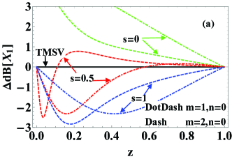
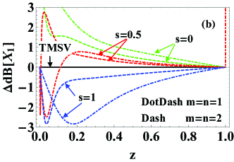
Figure 5: (Color online) The two-mode squeezing property $dB[X_{1}|_{\left|\psi\right\rangle}]$ as a function of squeezing parameter $z$ for different operator parameter $s=0,0.5,1$. for (a) the single-side GSP operations ($\left(m,n\right)\in\left\{\left(0,1\right),\left(0,2\right)\right\}$), (b) the two-side symmetric GSP operations ($\left(m,n\right)\in\left\{\left(1,1\right),\left(2,2\right)\right\}$). Solid lines correspond to the TMSV case.

To study the improvement of two-mode squeezing property between the GSP-TMSV and the initial TMSV, in Fig. 5, we plot the difference $\Delta$dB$[X_{1}]=$ $10\log_{10}\left[\left\langle\Delta X_{1}^{2}\right\rangle|_{\left|\psi\right\rangle_{ab}}/\left\langle\Delta X_{1}^{2}\right\rangle|_{TMSV}\right]$ as the function of $z$ with several superposition values $s=0,0.5,1$, including the single-side GSP operations ($\left(m,n\right)\in\{\left(0,1\right),(0,2)\}$) and the two-side symmetric GSP operations ($\left(m,n\right)\in\{\left(1,1\right),(2,2)\}$). In principle, the condition of $\Delta$dB$[X_{1}]<0$ means the existence and improvement of two-mode squeezing property, but $\Delta$dB$[X_{1}]\geqslant 0$ only indicates that two-mode squeezing property cannot be enhanced. It is interesting that, as for the two types of the GSP operations, the improved area of two-mode squeezing property for $s=0$ can not be shown, which means that using PS-then-PA operation on the TMSV makes it impossible to present the improvement of two-mode squeezing property. Whereas for other cases for $s=0.5$ and $1,$ the latter can always show the existence and improvement of two-mode squeezing property, and the improved area of two-mode squeezing property for the former would be limited at a small squeezing range. Besides, with the increase of $\left(m,n\right)$, this limitation is more obvious with respect to the narrower of achievable squeezing ranges. We also notice that, at a fixed $s,$ for the case of $s=0.5$, the achievable squeezing range for the single-side GSP operations are bigger than that for the two-side symmetric GSP operations in terms of the improvement of the two-mode squeezing property.

III Improvement of the QFI via the GSP-TMSV

After evaluating the nonclassical properties of the GSP-TMSV, then we consider whether the GSP-TMSV can be used to improve the QFI when the GSP-TMSV is used as inputs of the balanced MZI, which consists of two symmetrical beam splitters (BSs), shown in Fig. 1 (Box 2). In Ref. 51 , it is pointed out that the behavior of a BS can be described as a rotation, i.e., using the Schwinger representation of SU(2) algebra,

$$J_{1} = \frac{1}{2}\left(a^{\dagger}b+ab^{\dagger}\right),\text{ }J_{2}=\frac{1}{2i}\left(a^{\dagger}b-ab^{\dagger}\right),$$

$$J_{3} = \frac{1}{2}\left(a^{\dagger}a-b^{\dagger}b\right),\text{ }J_{0}=\frac{1}{2}\left(a^{\dagger}a+b^{\dagger}b\right),$$ (11)

where $J_{0}$ is a Casimir operator that commutes with all others angular momentum operators $\left[J_{i},J_{0}\right]=0$ $\left(i=1,2,3\right)$, which should satisfy the commutation relation $\left[J_{i},J_{j}\right]=i\varepsilon_{ijk}J_{k}$ $\left(i,j,k=1,2,3\right)$, then the action of the MZI can be equivalent to the following unitary operator

$$U\left(\varphi\right)=e^{i\pi J_{1}/2}e^{-i\varphi J_{3}}e^{-i\pi J_{1}/2}=e^{-i\varphi J_{2}}.$$ (12)

Thus, when inputting any pure state $\left|in\right\rangle$ into the MZI, the output state is given by

$$\left|out\right\rangle_{MZI}=e^{-i\varphi J_{2}}\left|in\right\rangle.$$ (13)

Combining Eqs. (2) and (13), for our scheme, the resulting state prior to the parity detection can be derived as

$$\left|out\right\rangle_{MZI}=\frac{\Re u}{\sqrt{P_{d}}}e^{a^{\dagger}b^{\dagger}v\cos\varphi+\frac{1}{2}(b^{\dagger 2}-a^{\dagger 2})v\sin\varphi}\left|00\right\rangle,$$ (14)

where we have used $e^{i\varphi J_{2}}\left|00\right\rangle=\left|00\right\rangle$ and the following transformation relations,

$$e^{-i\varphi J_{2}}a^{\dagger}e^{i\varphi J_{2}} = a^{\dagger}\cos\frac{\varphi}{2}+b^{\dagger}\sin\frac{\varphi}{2},$$

$$e^{-i\varphi J_{2}}b^{\dagger}e^{i\varphi J_{2}} = b^{\dagger}\cos\frac{\varphi}{2}-a^{\dagger}\sin\frac{\varphi}{2}.$$ (15)

In particular, for the case of $m=n=0$, Eq. (14) reduces to

$$\left|TMSV\right\rangle\text{=}\sqrt{1-z^{2}}e^{z[a^{\dagger}b^{\dagger}\cos\varphi+\frac{1}{2}(b^{\dagger 2}-a^{\dagger 2})\sin\varphi]}\left|00\right\rangle,$$ (16)

which is just the result in Ref. 8 , where the TMSV is used as inputs of the MZI, and the superresolution and sub-Heisenberg sensitivity can be achieved using parity detection. It is interesting that, due to the fact that the usefulness of non-Gaussian (PA- and PS-) operations for achieving the strongly nonclassical states, the PS(PA-)-based TMSV scheme has been proposed for further improving the measurement precision of quantum metrology. Then a question naturally arises: can our proposed GSP-TMSV scheme improve the phase sensitivity and resolution in quantum metrology?

Next, we first consider the proposed GSP-TMSV as the input of the MZI to study its QFI denoted by $F_{Q}$. The QFI is associated with the ultimate limit of phase sensitivity, which is given by the quantum Cramer-Rao boundary (QCRB) 52 , i.e.,

$$\Delta\phi_{\min}=\frac{1}{\sqrt{F_{Q}}}.$$ (17)

In particular, for any pure state $\left|\psi\left(\theta\right)\right\rangle,$ the QFI can be calculated as

$$F_{Q}=4\left\{\left\langle\psi^{{}^{\prime}}\left(\theta\right)\right|\left.\psi^{{}^{\prime}}\left(\theta\right)\right\rangle-\left|\left\langle\psi^{{}^{\prime}}\left(\theta\right)\right.\left|\psi\left(\theta\right)\right\rangle\right|^{2}\right\},$$ (18)

where $\left|\psi\left(\theta\right)\right\rangle=e^{-i\theta J_{3}}e^{-i\pi J_{1}/2}\left|in\right\rangle$ and $\left|\psi^{{}^{\prime}}\left(\theta\right)\right\rangle=\partial\left|\psi\left(\theta\right)\right\rangle/\partial\theta$. Thus, for the GSP-TMSV state shown in Eq. (2), the QFI can be directly calculated as

$$F_{Q}=2N\left(N+1\right)-\left\langle in\right|\left(a^{\dagger 2}b^{2}+a^{2}b^{\dagger 2}\right)\left|in\right\rangle,$$ (19)

where the APN $N$ has the same definition as Eq. (8) and the second term can be derived using Eq. (6). Especially, for the case of $m=n=0$ corresponding to the TMSV as inputs, Eq. (19) reduces to $F_{Q}$ $=4z^{2}/\left(1-z^{2}\right)^{2}$, as expected 22 .

According to Eq. (19), we illustrate the QFI as a function of $z$ for the single-side ($\left(m,n\right)\in\{\left(0,1\right),(0,2)\}$) and the two-side symmetric GSP operations ($\left(m,n\right)\in\{\left(1,1\right),(2,2)\}$), as shown in Figs. 6(a) and 6(b), respectively. It is obvious that the QFI using TMSV input (the black solid line) is outperformed by that using the GSP-TMSV for these two cases above. Specifically speaking, when given some parameters $s$ and $z$, the QFI of our scheme increases with the increase of $\left(m,n\right)$, especially for two-side symmetric GSP operations. The reason may be the fact that the APN of the GSP-TMSV increases as the increasing $\left(m,n\right)$ (see Fig. 2). In addition, at some fixed parameters $\left(m,n\right)$ and $z$, it is found that the QFI corresponding to the PS-then-PA operation ($s=0$) is always better than other cases, including $s=1$ and $s=0.5$. In addition, compared to the cases with $s=0$ and $s=0.5$, the QFI using PA-then-PS operation has a relatively poor improvement.

In order to highlight the advantages of the GSP-TMSV as the input of the MZI, we further make a comparison about the QFI for several different non-Gaussian states, such as single PA-TMSV (magenta dashed), single PS-TMSV (cayan dashed) and the GSP-TMSV with $m=n=1$. The QFI as a function of squeezing parameter $z$ is plotted in Fig. 7. It is interesting that both PA and PS operations always achieve an improvement of the QFI compared to the TMSV in the whole squeezing parameter region, while the PA operation presents a better performance than the PS operation. In addition, for the two cases with $s=1$ and $s=0.5$, the QFI can be also improved when the squeezing parameter exceeds a small threshold. The latter with $s=0.5$ performs better than the former with $s=1.$ However, among these non-Gaussian operations, the PS-then-PA operation ($s=0$) presents the best improvement in the whole squeezing parameter region. These results are similar to the APN cases of different (non-)Gaussian states (see Fig.3).

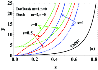
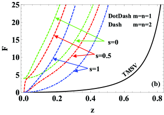
Figure 6: (Color online) Plots of the quantum Fisher information $F_{Q}$ against the squeezing parameter $z$ for different operator parameter $s=0,0.5,1$. for (a) the single-side GSP operations ($\left(m,n\right)\in\left\{\left(0,1\right),\left(0,2\right)\right\}$), (b) the two-side symmetric GSP operations ($\left(m,n\right)\in\left\{\left(1,1\right),\left(2,2\right)\right\}$). Solid lines correspond to the TMSV case.

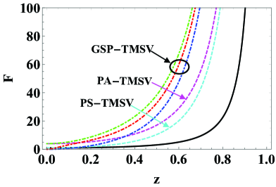
Figure 7: (Color online) As a comparison, the QFI $F_{Q}$ as a function of the squeezing parameter $z$. The dot-dashed lines represent our scheme for operation parameter $s=0,0.5,1$ (corresponding to green, red, and blue color line, respectively.), and dashed lines represent the previous work of performing the PA-TMSV (magenta color line) and the PS-TMSV (cyan color line). Solid line corresponds to the TMSV case.

IV Phase estimation with parity detection

In this section, we considered the QFI, which corresponds to the upper bound of measurement preision. Actually, the practical precision depends on the way of measure. In this section, we further examine the phase estimation using special measures. Note that the parity detection has advantages over the other detection schemes, thus here we shall take the parity detection as a powerful tool for analyzing the phase sensitivity of our scheme.

IV.1 The parity detection

In fact, the aim of parity detection is to obtain the expectation value of the parity operator in the output state of the MZI 53 , which plays a vital role in quantum measurements. In particular, when the TMSV is used as the input, the parity detection can effectively extract the phase information, while the intensity detection is not applicable 45 . For convenience, we choose the $b$ mode of the output, then the parity operator can be written as

$$\Pi_{b}=e^{i\pi b^{\dagger}b}=\int\frac{d^{2}\gamma}{\pi}\left|\gamma\right\rangle\left\langle-\gamma\right|,$$ (20)

where $\left|\gamma\right\rangle$ is the coherent state, such that for an arbitrary output state $\rho_{out}=\left|out\right\rangle_{MZI}\left\langle out\right|$ in the MZI, the corresponding expectation value of $\Pi_{b}$ can be expressed as

$$\left\langle\Pi_{b}\right\rangle=\mathtt{Tr}[\Pi_{b}\rho_{out}]=\int\frac{d^{2}\gamma}{\pi}\left\langle-\gamma\right|\rho_{out}\left|\gamma\right\rangle.$$ (21)

Thus, based on Eq. (13), the expectation value $\left\langle\Pi_{b}\right\rangle$ can be calculated as

$$\left\langle\Pi_{b}(\varphi)\right\rangle=\widetilde{\Re}\frac{uu_{1}\Omega_{1}}{P_{d}\sqrt{\Omega_{2}-\Omega_{3}}},$$ (22)

with

$$\Omega_{1} = \left(1-v_{1}v\sin^{2}\varphi\right)^{\frac{1}{2}},$$

$$\Omega_{2} = \left(v_{1}v\cos 2\varphi+1\right)^{2},$$

$$\Omega_{3} = v_{1}v\left(vv_{1}-1\right)^{2}\sin^{2}\varphi.$$ (23)

In particular, when $m=n=0,$ Eq. (22) reduces to $\left\langle\Pi_{b}(\varphi)\right\rangle=\left(1-z^{2}\right)/\sqrt{\left(1-2z^{2}\cos 2\phi+z^{4}\right)}$ ($\varphi=\phi+\pi/2$), corresponding to the TMSV case, as expected 8 . In the following, we will use the variable $\phi$ to investigate the resolution and sensitivity.

In Ref. 8 , it has been shown that the central peak of $\left\langle\Pi_{b}(\phi+\pi/2)\right\rangle$ at $\phi=0$ for the TMSV inputs is narrower than that for the coherent state input under the same parameters, thereby achieving superresolution and sub-Heisenberg sensitivity of the MZI. However, it is interesting that the case can be further improved using our scheme. For given squeezing parameter $z=0.6,$ using Eq. (22) we illustrate the expectation values $\left\langle\Pi_{b}(\phi+\pi/2)\right\rangle$ as a function of the phase shift $\phi$ in Fig. 8, including both the single-side GSP operations ($\left(m,n\right)\in\{\left(0,1\right),(0,2)\}$ in Fig. 8(a)) and the two-side symmetric GSP operations ($\left(m,n\right)\in\left\{\left(1,1\right),\left(2,2\right)\right\}$ in Fig. 8(b)).

From Fig. 8, it is clear that the central peak of $\left\langle\Pi_{b}(\phi+\pi/2)\right\rangle$ at $\phi=0$ for all the GPS-TMSV inputs is much narrower than that for the TMSV input. It implies that the use of the GSP operation is beneficial for significantly increasing the superresolution. Among these non-Gaussian operations, the PS-then-PA operation ($s=0$) presents the best performance again. In addition, for both the single-side (Fig. 8(a)) and two-side (Fig. 8(b)) GSP operations, the resolution can be further enhanced by increasing the parameter $\left(m,n\right)$. Compared to the single-side case, the two-side case has a better performance for the improvement of superresolution under the same parameters.

In Fig. 9, we make a comparison about $\left\langle\Pi_{b}(\phi+\pi/2)\right\rangle$ between single PA(PS)-TMSVs and our proposed scheme with $m=n=1$ for a given squeezing parameter $z=0.6$. It is obvious that these non-Gaussian operations can effectively enhance the resolution and the effects of improvement can be ranked from small to large, i.e., PS, PA, PA-then-PS ($s=1$), PA-then-PS plus PS-then-PA ($s=0.5$), and PS-then-PA ($s=0$). Thus, compared to both PA and PS, our scheme presents the advantages for further improving superresolution, especially for PS-then-PA $(s=0).$

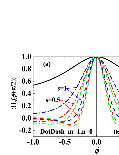
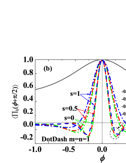
Figure 8: (Color online) The expectation values of the parity operator $\left\langle\Pi_{b}(\phi+\pi/2)\right\rangle$ versus the phase shift $\phi$ for a given squeezed parameter $z=0.6$ and different operator parameter $s=0,0.5,1$. (a) the single-side GSP operations ($\left(m,n\right)\in\left\{\left(0,1\right),\left(0,2\right)\right\}$), (b) the two-side symmetric GSP operations ($\left(m,n\right)\in\left\{\left(1,1\right),\left(2,2\right)\right\}$). Solid lines correspond to the TMSV case.

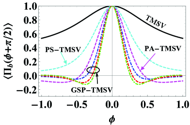
Figure 9: (Color online) The expectation values of the parity operator $\left\langle\Pi_{b}(\phi+\pi/2)\right\rangle$ as a function of $\phi$ for fixed squeezed parameter $z=0.6$ for different non-Gaussian operations. The dot-dashed lines represent the our work for operation parameter $s=0,0.5,1$ (green, red, and blue color line, respectively.), and dashed lines represent the previous work performing the PA (magenta color line) and the PS operations (cyan color line). Solid line corresponds to the TMSV case.

IV.2 The phase sensitivity

After investigating the resolution of our scheme in the MZI, in this subsection, we further consider the sensitivity of phase estimation based on the outcome of parity detection. In general, the phase sensitivity of the MZI can be estimated by the error propagation formula 54 ; 55 , i.e.,

$$\Delta\phi=\frac{\sqrt{1-\left\langle\Pi_{b}(\varphi)\right\rangle^{2}}}{|\partial\Pi_{b}/\partial\phi|}.$$ (24)

In particular, when $m=n=0$ corresponding to the case of TMSV input, using Eq. (22) then Eq. (24) reduces to $\Delta\phi_{TMSV}=\left(1-2z^{2}\cos 2\phi+z^{4}\right)/\left\{[2z(1-z^{2})\cos\phi]\right\},$ as expected. At the limitation of $\phi\rightarrow 0,$ $\Delta\phi_{TMSV}$ becomes $\Delta\phi_{\min}=\left(1-z^{2}\right)/\left(2z\right)=1/\sqrt{F_{Q}}$, in which $F_{Q}$ is the QFI for the TMSV input into the MZI. This indicates that the QCRB can be achieved especially at $\phi\rightarrow 0$ with the help of the parity detection.

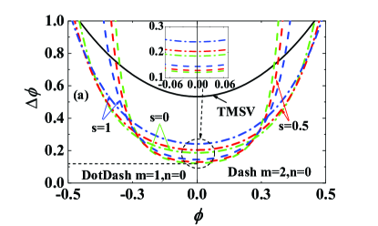
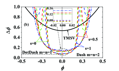
Figure 10: (Color online) The phase uncertainty $\Delta\phi$ versus the phase shift $\phi$ for a given squeezed parameter $z=0.6$ and different operator parameter $s=0,0.5,1$. (a) the single-side GSP operations ($\left(m,n\right)\in\left\{\left(0,1\right),\left(0,2\right)\right\}$), (b) the two-side symmetric GSP operations ($\left(m,n\right)\in\left\{\left(1,1\right),\left(2,2\right)\right\}$). Solid lines correspond to the TMSV case.

Generally, the lower the value $\Delta\phi$, the higher the phase sensitivity. In order to clearly see the effects of different parameters on the phase sensitivity, at fixed values of $z=0.6$ and $s=0,0.5,1$, we plot the phase sensitivity$\ \Delta\phi$ as a function of the phase $\phi$ for the single-side ($\left(m,n\right)\in\{\left(0,1\right),(0,2)\}$) and the two-side ($\left(m,n\right)\in\left\{\left(1,1\right),\left(2,2\right)\right\}$) symmetric GSP operations in Fig. 10(a) and 10(b), respectively. Compared to the TMSV case, the minimum value of $\Delta\phi_{\min}$ can be significantly reduced by single- and two-side cases above. For given parameter $s$, the $\Delta\phi_{\min}$ can be further decreased with the increasing of the parameters $\left(m,n\right)$. Comparing single-side case with two-side case (Fig. 10(a) and 10(b)), it is clear that the latter can achieve a lower $\Delta\phi_{\min}$ than the former. In addition, the PS-then-PA ($s=0$) is the best operation for getting the minimum value $\Delta\phi$ under the condition that other parameters are the same.

In Fig. 11, we further make a comparison about $\Delta\phi_{\min}$ between single PA(PS)-TMSVs and our proposed scheme, where the condition is the same as that in Fig. 10. In terms of minima $\Delta\phi_{\min},$ the effects for these non-Gaussian operations can be ranked from large to small, i.e., PS, PA, PA-then-PS ($s=1$), PA-then-PS plus PS-then-PA ($s=0.5$), and PS-then-PA ($s=0$). Again, the PS-then-PA is the best choice for achieving the minima of $\Delta\phi_{\min}$ due to the fact that the APN can be increased by the PS-then-PA. These results indicate that under the same parameters the phase sensitivity $\Delta\phi$ can be further enhanced by using our scheme when comparing to the PA-TMSV and the PS-TMSV.

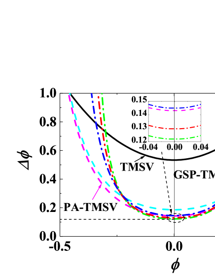
Figure 11: (Color online) As a comparison, the phase uncertainty $\Delta\phi$ as a function of the phase shift $\phi$ for fixed squeezed parameter $z=0.6.$ The dot-dashed lines represent the our work for operation parameter $s=0,0.5,1$ (corresponding to green, red, and blue color line, respectively.), and dashed lines represent the previous work of performing the PA-TMSV (magenta color line) and the PS-TMSV (cyan color line). Solid line corresponds to the TMSV case

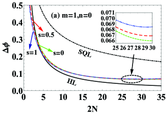
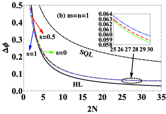
Figure 12: (Color online) The phase sensitivity$\ \Delta\phi$ as a function of the total APN $2N$ for different operator parameter $s=0,0.5,1$. for (a) the single-side GSP operations ($\left(m,n\right)\in\left(0,1\right)$), (b) the two-side symmetric GSP operations ($\left(m,n\right)\in\left(1,1\right)$). Solid lines correspond to the TMSV case.

On the other hand, it is interesting to notice that the HL based on parity detection can be beaten when the TMSV is considered as the input of the MZI 8 . However, when the PA-TMSV or PS-TMSV is used as inputs, the HL cannot be beaten and the corresponding phase uncertainties perform worse compared to the TMSV under the same parameters 22 . Then how about our scheme? In order to clearly see this point, for given phase $\phi=0.05$ and $s=0,0.5,1$, we show the phase sensitivity as function of the total APN $2N$ for single-side ($\left(m,n\right)\in\left(1,0\right)$) and two-side symmetric GSP operations ($\left(m,n\right)\in\left(1,1\right)$) in Figs. 12(a) and 12(b), respectively. For our scheme, it is shown that the SQL is always broken through due to the fact that the GSP-TMSV is a kind of nonclassical state. As discussed above, the PS-then-PA ($s=0$) can be used to achieve the best phase sensitivity and superresolution, however, the HL cannot be beaten by this case, but by the cases of $s=0.5,1$ in the regime of the small total APN (or say, the small initial squeezing parameter $z$). The reason may be that, except for $s=0,$ the two-mode squeezing property can be always improved for the cases of $s=0.5,1$ at the certain range of $z,$ which can be seen from Fig. 5. In addition, it is also interesting to notice that, for the cases of $s=0.5,1$, it is much significant for beating the HL using single-side GSP operation $\left(m,n\right)\in\left(1,0\right)$ rather than two-side GSP operation $\left(m,n\right)\in\left(1,1\right)$ at small range of the total APN. While in the larger total APN region, two-side GSP operation is much easier to make the phase uncertainty close to the HL, which is beneficial for the practical implementation of achieving the super-sensitivity.

V Effects of photon losses on phase sensitivity

In practice, the travelling states are inevitably coupled to the environment, so that the decoherence process should be taken into account. Generally, there are several models of decoherence processes, such as photon loss, phase diffusion and thermal noise. As described in Ref. 56 , particularly, it is shown that the photon losses have a significant impact on phase sensitivity. Thus, here we only consider the effects of photon loss for $\left(m,n\right)=\left(1,1\right)$ and $z=0.6$ in our scheme, including external and internal losses shown in Figs. 13(a) and 13(b), respectively. For this season, in the following simulations, we shall give more detailed analysis for our scheme about the effects of photon losses on the superresolution and the phase sensitivity. For simplicity, the relevant calculation details are not shown here, please refer to the appendix A.

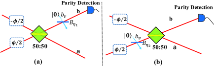
Figure 13: (Color online) Schematic diagram of the photon losses (a) in front of the parity detection (denoted as an external loss) and (b) between the phase shifter and the second BS (denoted as an internal loss).

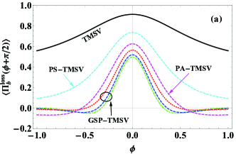
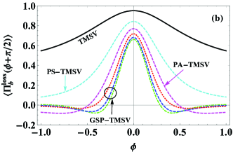
Figure 14: (Color online) The expectation values of the parity operator $\left\langle\Pi_{b}(\phi+\pi/2)\right\rangle$ with (a) external losses and (b) internal losses as a function of $\phi$ for some fixed parameter $z=0.6$, $\eta_{1}=\eta_{2}=0.9$ and $m=n=1$. The dot-dashed lines represent the our work for several different $s=0,0.5,1$ (corresponding to green, red, and blue dot-dashed line, respectively). As a comparison, dashed lines represent the previous work performing the PA (magenta color line) and the PS operations (cyan color line). Solid line corresponds to the TMSV case.

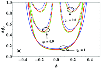
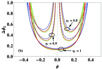
Figure 15: (Color online) The phase sensitivity with (a) external losses and (b) internal losses$\ \Delta\phi_{L}$ as a function of $\phi$ at some fixed parameter $z=0.6$ and $m=n=1$ for several dissipation values $\eta_{1}=\eta_{2}=1,0.9,0.8$ and $s=0,0.5,1$ (corresponding to green, red, and blue dot-dashed lines, respectively.) As a comparison, the solid line corresponds to the ideal cases, the dot-dashed and dashed lines represent $\eta_{1}=\eta_{2}=0.9$ and $\eta_{1}=\eta_{2}=0.8$, respectively.

In Fig. 14, at a fixed dissipation value $\eta_{1}=\eta_{2}=0.9$, we show the expectation values $\left\langle\Pi_{b}^{loss}(\phi+\pi/2)\right\rangle$ with the external- and internal- losses as a function of the phase shift $\phi$ for several different parameters $s=0,0.5,1.$ It is clear that the photon-loss processes make the central peak of $\left\langle\Pi_{b}^{loss}(\phi+\pi/2)\right\rangle$ at $\phi=0$ lower than that of $\left\langle\Pi_{b}(\phi+\pi/2)\right\rangle$ for the ideal cases (see Fig. 9). Nevertheless, we can see that the central peaks of $\left\langle\Pi_{b}^{loss}(\phi+\pi/2)\right\rangle$ at $\phi=0$ for all the GPS-TMSV inputs are much narrower than that for both the TMSV and the single PA(PS)-TMSVs inputs, which reveals that the GPS operations, especially for PS-then-PA $(s=0),$ help to increase the superresolution even in the presence of photon losses, compared to both PA and PS. Besides, in contrast to the external-loss cases, the central peaks of $\left\langle\Pi_{b}^{loss}(\phi+\pi/2)\right\rangle$ for the internal losses at $\phi=0$ are relatively narrower, which implies that the external losses have a greater influence on the superresolution than the internal ones.

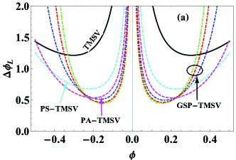
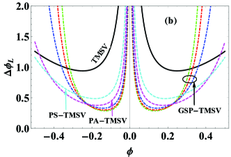
Figure 16: (Color online) The phase sensitivity$\ \Delta\phi_{L}$ with (a) external losses and (b) internal losses as a function of $\phi$ for some fixed parameters $z=0.6,m=n=1$ and $\eta_{1}=\eta_{2}=0.9$. The dot-dashed lines represent the our work for several different $s=0,0.5,$ and $1$ (corresponding to green, red, and blue dot-dashed lines, respectively). As a comparison, dashed lines represent the previous work performing the PA (magenta color line) and PS operations (cyan color line). Black solid line corresponds to the TMSV case.

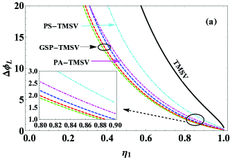
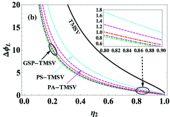
Figure 17: (Color online) The phase sensitivity with (a) external-losses and (b) internal-losses as a function of transmissivity of fictitious beam splitter $\eta_{1}($or $\eta_{2})$ for some fixed parameters $z=0.6,$ $\phi=0.05$ and $s=0,0.5,1$ (green, red, and blue dot-dashed lines, respectively). As a comparison, black solid line corresponds to the TMSV case. Cyan- and purple dashed lines correspond to the PS-TMSV and the PA-TMSV, respectively.

To visually display the effects of photon losses on phase sensitivity, we illustrate the phase sensitivity$\ \Delta\phi_{L}$ as a function of the phase $\phi$ for several dissipation values $\eta_{l}=1,0.9,0.8$ $(l=1,2),$ as shown in Fig. 15. The solid lines represent the ideal case with $\eta_{l}=1$ where the optimal phase point is at $\phi_{opt}=0$. However, in the presence of photon losses, the optimal phase point that tends to be far away from zero for $\eta_{l}=$ $0.9,0.8$ is at $\phi_{opt}\neq 0,$ which leads to the decrease of phase sensitivity. The reason may be that the noise could be suppressed in near decorrelation point ($\phi=0$), as shown in Ref. 57 . Furthermore, under the same accessible parameters except for $\eta_{l}=1$, the phase sensitivity $\Delta\phi_{L}$ for the internal losses performs better than that for the external-loss cases, which indicates that the latter has a greater impact on the precision of phase measurement. In order to show the advantages of our scheme, on the other hand, we take a fixed $\eta_{l}=0.9$ and make a comparison about $\Delta\phi_{L}$ changing with the phase $\phi$ for several non-Gaussian resources inputs involving single PA(PS)-TMSVs and GSP-TMSV, as shown in Fig. 16. It is found that, compared with the TMSV input (black solid line), these non-Gaussian resources can still be used for enhancing the phases sensitivity even in the presence of photon losses. Among them, all the GSP-TMSV inputs, present better advantages for further improving the phases sensitivity when considering photon losses, in which the PS-then-PA $(s=0)$ is the best.

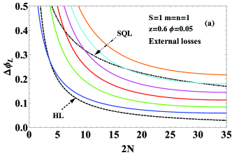
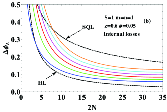
Figure 18: (Color online) The phase sensitivity$\ \Delta\phi_{L}$ with (a) external-losses and (b) internal-losses as a function of the total APN $2N$ at some fixed parameters $s=1,m=n=1$ and $\phi=0.05$. The dot-dashed and dashed line correspond to the SQL and HL, respectively. The color lines from down to up correspond to dissipation value $\eta_{1}=\eta_{2}=1,0.99,0.98,0.97,0.96,$ and $0.95$, respectively.

In Fig. 17, we plot the phase sensitivity $\Delta\phi_{L}$ as a function of $\eta_{1}($or $\eta_{2})$ for several non-Gaussian resources inputs mentioned above at fixed parameters $z=0.6$ and $\phi=0.05$, from which the phase sensitivity can be deteriorated severely with the decrease of $\eta_{1}($or $\eta_{2}).$ In contrast to the TMSV input, fortunately, the phases sensitivity can be still improved even in the presence of photon losses by using these non-Gaussian resources, especially for the GSP-TMSV. In this sense, this means that the GSP operations are more effective to resist photon losses comparing with the PA(PS) operation. In addition, the effects of the external losses on phase sensitivity are more serious than the internal-loss cases, particularly in the small $\eta_{1}($or $\eta_{2})$ regimes.

On the other hand, as shown in Fig. 12, without losses, it is shown that the SQL can be broken for all the GSP-TMSV inputs and the HL for the cases of $s=0.5,1$ can be beaten in the regime of the small total APN. In the context of photon losses, then, can the two limits be broken by using the GSP-TMSV? To this end, for some given parameters $\left(m,n\right)=\left(1,1\right),z=0.6$ and $\phi=0.05,$ in Fig. 18, we plot the phase sensitivity $\Delta\phi_{L}$ as a function of total APN $2N$ for several dissipation values $\eta_{l}=1,0.99,0.98,0.97,0.96$ and $0.95$. It is clearly seen that the phase sensitivity decreases rapidly with the decrease of $\eta_{1}($or $\eta_{2}).$ Particularly, when $\eta_{1}=0.95,$ the SQL cannot be achieved for the external-loss cases but can be still broken through at large range of the total APN for the internal-loss ones. These results indicate that the external losses make against to the effective improvement of phase sensitivity compared to the internal-loss cases.

VI Conclusion

In summary, we propose a scheme to improve the phase sensitivity and resolution using a novel non-Gaussian quantum state, the GSP-TMSV, as the input of the MZI via parity detection. The nonclassicality of the proposed state is discussed in terms of the APN, the anti-bunching effect and two-mode squeezing property. We also investigate both the QFI and the phase resolution/sensitivity based on parity detection when using GSP-TMSV as input in detail. The numerical results show that our scheme, especially for the case of the PS-then-PA TMSV, is always superior to the original TMSV scheme in terms of the QFI and the phase resolution and sensitivity, which is caused by the fact that the total APN of the former is larger than that of the latter.

In addition, to show the advantages of our scheme, we also make comparisons between the GSP-TMSV and the previous PA(or PS)-TMSV schemes in terms of the total APN, the QFI, and the phase resolution and sensitivity. The results indicate that the current scheme can surpass the previous schemes, especially when the PS-then-PA TMSV is used. This means that the proposed GSP operation can obviously improve the QFI and the phase resolution and sensitivity. In addition, comparing with the single-side GSP operations, the improvement of phase sensitivity via two-side symmetric ones is more remarkable under the same accessible parameters. Furthermore, the SQL can always be surpassed by our scheme and the HL can be beaten when $s=0.5,1$ in the regime of the small total APN, but not by the case of $s=0$. These results show that the GSP-TMSV is an useful resource for improving phase sensitivity remarkably beyond the classical limit, and even going beyond the HL.

From a realistic point of view, we also study the sensitivity of phase estimation with parity detection in the presence of photon losses, including external- and internal- losses. The results indicate that compared with the internal photon losses, the external ones have a greater impact on phase sensitivity when several non-Gaussian resources, involving single PA(PS)-TMSVs and GSP-TMSV, are used as the inputs. Dramatically, under the same parameters, the phase sensitivity with the GSP-TMSV, especially for the case of $s=0$, can be better than those base on the TMSV or the PA(PS)-TMSV in the presence of photon losses. Besides, it is also noted that in the presence of photon losses, the HL cannot be beaten, but fortunately the SQL can still be surpassed when GSP-TMSV is used as the inputs particularly when the total APN is large. Our results shown here can find important applications in quantum metrology.

Appendix A: Derivation of the phase sensitivity with parity detection in the presence of photon losses

In order to derive the phase sensitivity with parity detection in the presence of photon losses, for simplicity, here we consider two special photon-loss processes, i.e., the external loss and the internal one, shown in Fig. 13. In practice, the photon losses on auxiliary mode $b_{v}$ can be structured using a fictitious beam splitter (denoted as $B_{\eta_{i}}$) with a dissipation factor $\eta_{i}$ ($i=1$ and $2$ corresponding to the external and internal losses, respectively), whose transform relation is given by 58a

$$B_{\eta_{i}}^{\dagger}\binom{b}{b_{v}}B_{\eta_{i}}=\left(\begin{array}[]{cc}\sqrt{\eta_{i}}&\sqrt{1-\eta_{i}}\\ -\sqrt{1-\eta_{i}}&\sqrt{\eta_{i}}\end{array}\right)\binom{b}{b_{v}}.$$ (A1)

It is worth mentioning that the smaller the values of $\eta_{i}$, the more severe the photon losses. Particularly, $\eta_{i}=1$ corresponds to the ideal case. To get the parity operator in the presence of the external losses, on one hand, it is necessary to rewrite Eq. (20) under the Weyl ordering representation 58 , i.e.,

$$\Pi_{b}=\frac{\pi}{2}\begin{array}[]{c}:\\ :\end{array}\delta\left(b\right)\delta\left(b^{\dagger}\right)\begin{array}[]{c}:\\ :\end{array},$$ (A2)

where $\begin{array}[]{c}:\\ :\end{array}\bullet\begin{array}[]{c}:\\ :\end{array}$ denotes the symbol of the Weyl ordering and $\delta\left(\bullet\right)$ denotes the delta function. Thus, by using Eq. (A1), one can obtain the parity operator with external losses (denoted as $\Pi_{b}^{loss}$), namely,

$$\Pi_{b}^{loss} \text{=}\frac{\pi}{2}_{v}\left\langle 0\right|\begin{array}[]{c}:\\ :\end{array}\delta\left(\sqrt{\eta_{i}}b+\sqrt{1-\eta_{i}}b_{v}\right)$$ (25c)

$$\times\delta\left(\sqrt{\eta_{i}}b^{\dagger}+\sqrt{1-\eta_{i}}b_{v}^{\dagger}\right)\begin{array}[]{c}:\\ :\end{array}\left|0\right\rangle_{v},$$ (A3)

where $$\left|0\right\rangle_{v} b_{v}$$ is the vacuum noise input on auxiliary mode . Finally, according to the classical correspondence of the operator

$$\begin{array}[]{c}:\\ :\end{array}f\left(b,b^{\dagger},b_{v},b_{v}^{\dagger}\right)\begin{array}[]{c}:\\ :\end{array} \text{=}4\int d^{2}\beta d^{2}\gamma f\left(\beta,\beta^{\ast},\gamma,\gamma^{\ast}\right)$$ (26e)

$$\times\Delta\left(\beta,\beta^{\ast}\right)\Delta\left(\gamma,\gamma^{\ast}\right),$$ (A4)

with Wigner operators under the normal ordering 59

$$\Delta\left(\beta,\beta^{\ast}\right) =\colon\exp\left[-2(b^{\dagger}-\beta^{\ast})(b-\beta)\right]\colon,$$

$$\Delta\left(\gamma,\gamma^{\ast}\right) =\colon\exp\left[-2(b_{v}^{\dagger}-\gamma^{\ast})(b_{v}-\gamma)\right]\colon,$$ (A5)

and using the IWOP technique 60 , it is easy to obtain

$$\Pi_{b}^{loss}=\colon e^{-2\eta_{1}b^{\dagger}b}\colon=\left(1-2\eta_{1}\right)^{b^{\dagger}b},$$ (A6)

where the symbol $\colon\colon$ denotes the normal ordering. Thus, combining Eqs. (14) and (A6), the average value of $\Pi_{b}^{loss}$ for the output state can be given by

$$\left\langle\Pi_{b}^{loss}\right\rangle=\text{Tr}\left[\rho_{out}\Pi_{b}^{loss}\right]=\widetilde{\Re}\frac{uu_{1}\sqrt{\vartheta_{1}}}{P_{d}\sqrt{\vartheta_{2}^{2}-\vartheta_{3}}},$$ (A7)

with

$$\vartheta_{1} =1-vv_{1}\sin^{2}\varphi,$$

$$\vartheta_{2} =1-vv_{1}+2\eta_{1}v_{1}v\cos^{2}\varphi,$$

$$\vartheta_{3} =\left(1-2\eta_{1}\right)^{2}\sin^{2}\varphi v_{1}v\left(1-vv_{1}\right)^{2}.$$ (A8)

On the other hand, different from the derivation of Eq. (A6), we rewrite the parity operator with the internal losses as

$$\widetilde{\Pi}_{b}^{loss} \text{=}_{v}\left\langle 0\right|B_{1}^{\dagger}U^{\dagger}\left(\varphi\right)B_{v}^{\dagger}B_{2}^{\dagger}e^{i\pi b^{\dagger}b}B_{2}B_{v}U\left(\varphi\right)B_{1}\left|0\right\rangle_{v}$$

$$\text{=}\colon e^{\varpi_{1}a^{\dagger}a-\varpi_{2}b^{\dagger}a-\varpi_{2}^{\ast}a^{\dagger}b+\varpi_{3}b^{\dagger}b}\colon,$$ (A9)

where $$U\left(\varphi\right)$$ is given in Eq. (12) and

$$\varpi_{1} =\sqrt{\eta_{2}}\cos\varphi-\frac{1+\eta_{2}}{2},$$

$$\varpi_{2} =\frac{\left(\eta_{2}+1\right)^{2}-4\eta_{2}\cos^{2}\varphi}{4\left(i\eta_{2}-i+2\sqrt{\eta_{2}}\sin\varphi\right)},$$

$$\varpi_{3} =-\sqrt{\eta_{2}}\cos\varphi-\frac{1+\eta_{2}}{2},$$ (A10)

as well as we have used the following transformation relationships

$$B_{1}^{\dagger}\left(\begin{array}[]{c}a\\ b\end{array}\right)B_{1} =\frac{\sqrt{2}}{2}\left(\begin{array}[]{cc}1&i\\ i&1\end{array}\right)\left(\begin{array}[]{c}a\\ b\end{array}\right),$$ (31g)

$$B_{2}^{\dagger}\left(\begin{array}[]{c}a\\ b\end{array}\right)B_{2} =\frac{\sqrt{2}}{2}\left(\begin{array}[]{cc}1&-i\\ -i&1\end{array}\right)\left(\begin{array}[]{c}a\\ b\end{array}\right).$$ (A11)

Thus, for a given input GSP-TMSV, one can obtain the expectation value of $$\widetilde{\Pi}_{b}^{loss}$$ for the internal losses, i.e.,

$$\left\langle\Pi_{b}^{loss}\right\rangle =\mathtt{Tr}[\left|\psi\right\rangle_{ab}\left\langle\psi\right|\widetilde{\Pi}_{b}^{loss}]$$

$$=\frac{\widetilde{\Re}uu_{1}}{p_{d}}\left[\left(1-\omega_{1}\right)^{2}-\omega_{2}\right]^{-\frac{1}{2}},$$ (A12)

with

$$\omega_{1} =v_{1}v\left(\varpi_{1}\varpi_{3}-\eta_{2}+\left|\varpi_{2}\right|^{2}\right),$$

$$\omega_{2} =4\left|\varpi_{2}\right|^{2}v_{1}^{2}v^{2}\left(\varpi_{1}\varpi_{3}-\eta_{2}\right).$$ (A13)

Finally, using Eqs. (A7) and (A12), the phase sensitivity (denoted as $$\Delta\phi_{L}$$) in the presence of external and internal losses can be estimated by the error propagation formula

$$\Delta\phi_{L}=\frac{\sqrt{1-\left\langle\Pi_{b}^{loss}\right\rangle^{2}}}{\left|\partial\Pi_{b}^{loss}/\partial\phi\right|}.$$ (A14)

References

- (1) S. L. Braunstein and C. M. Caves, Statistical Distance and the Geometry of Quantum States, Phys. Rev. Lett. 72, 3439 (1994).
- (2) J. P. Dowling, Quantum optical metrology-the lowdown on high-N00N states, Contem. Phys. 49, 125 (2008).
- (3) J. J . Bollinger, W. M. Itano, and D. J. Wineland, Optimal frequency measurements with maximally correlated states, Phys. Rev. A 54, 4649 (1996)
- (4) V. Giovannetti, S. Lloyd, and L. Maccone, Advances in quantum metrology, Nat. Photonics 5, 222 (2011).
- (5) C. M. Caves, Quantum-mechanical noise in an interferometer, Phys. Rev. D 23, 1693 (1981).
- (6) R. Carranza and C. C. Gerry, Photon-subtracted two-mode squeezed vacuum states and applications to quantum optical interferometry, J. Opt. Soc. Am. B 29, 2581 (2012).
- (7) H. Kwon, K. C. Tan, T. Volkoff, and H. Jeong, Nonclassicality as a Quantifiable Resource for Quantum Metrology, Phys. Rev. Lett. 122, 040503 (2019).
- (8) P. M. Anisimov, G. M. Raterman, A. Chiruvelli, W. N. Plick, S. D. Huver, Quantum Metrology with Two-Mode Squeezed Vacuum: Parity Detection Beats the Heisenberg Limit, Phys. Rev. Lett. 104, 103602 (2010).
- (9) I. Afek, O. Ambar, and Y. Silberberg, High-NOON States by Mixing Quantum and Classical Light, Science 328, 879 (2010).
- (10) V. Giovannetti, S. Lloyd, and L. Maccone, Quantum-Enhanced Measurements: Beating the Standard Quantum Limit, Science 306, 1330 (2004).
- (11) J. Joo, W. J. Munro, and T. P. Spiller, Quantum Metrology with Entangled Coherent States, Phys. Rev. Lett. 107, 083601 (2011).
- (12) M. Jarzyna and R. D. Dobrzański, Quantum interferometry with and without an external phase reference Phys. Rev. A 85, 011801 (2012).
- (13) J. J. Cooper, D. W. Hallwood, J. A. Dunningham, and J. Brand, Robust Quantum Enhanced Phase Estimation in a Multimode Interferometer, Phys. Rev. Lett. 108, 130402 (2012).
- (14) T. Eberle, V. Hadchen, and R. Schnabel, Stable control of 10 dB two-mode squeezed vacuum states of light, Opt. Express 21, 11546 (2013).
- (15) N. Namekata, Y. Takahashi, G. Fujii, D. Fukuda, S. Kurimura, and S. Inoue, Non-Gaussian operation based on photon subtraction using a photon-number-resolving detector at a telecommunications wavelength, Nature Photonics 10, 1038 (2010).
- (16) L. Y. Hu, Z. Y. Liao, and M. S. Zubairy, Continuous-variable entanglement via multiphoton catalysis, Phys. Rev. A 95, 012310 (2017).
- (17) L. Y. Hu, M. Al-amri, Z. Y. Liao, and M. S. Zubairy, Entanglement improvement via a quantum scissor in a realistic environment, Phys. Rev. A 100, 052322 (2019).
- (18) G. S. Agarwal and K. Tara, Nonclassical properties of states generated by the excitations on a coherent state. Phys. Rev. A 43, 492 (1991).
- (19) A Zavatta, V. Parigi, and M Bellini, Experimental nonclssicality of single-photon-added thermal light states. Phys. Rev. A 75, 052106 (2007).
- (20) L. Y. Hu and Z. M. Zhang, Statistical properties of coherent photon-added two-mode squeezed vacuum and its inseparability, J. Opt. Soc. Am. B 30, 518 (2013)
- (21) A. Zavatta, S. Viciani, and M. Bellini, Quantum-to-classical transition with single-photon-added coherent states of light, Science 306, 660–662 (2004).
- (22) Y. Ouyang, S. Wang, and L. J. Zhang, Quantum optical interferometry via the photon added two-mode squeezed vacuum states, J. Opt. Soc. Am. B 33, 1373 (2016).
- (23) S. Y. Lee, S. W. Ji, H. J. Kim, and H. Nha, Enhancing quantum entanglement for continuous variables by a coherent superposition of photon subtraction and addition, Phys. Rev. A 84, 012302 (2011).
- (24) S. Wang, L. L. Hou, X. F. Chen, and X. F. Xu, Continuous-variable quantum teleportation with non-Gaussian entangled states generated via multiple-photon subtraction and addition, Phys. Rev. A 91, 063832 (2015).
- (25) E. D. Lopaeva, I. R. Berchera, I. P. Degiovanni, S. Olivares, G. Brida, and M. Genovese, Experimental Realization of Quantum Illumination, Phys. Rev. Lett. 110, 153603 (2013).
- (26) S. H. Tan, B. I. Erkmen, V. Giovannetti, S. Guha, S. Lloyd, L. Maccone, S. Pirandola, and J. H. Shapiro, Quantum Illumination with Gaussian States, Phys. Rev. Lett. 101, 253601 (2008).
- (27) Y. Guo, W. Ye, H. Zhong, and Q. Liao, Continuous-variable quantum key distribution with non-Gaussian quantum catalysis, Phys. Rev. A 99, 032327 (2019).
- (28) W. Ye, H. Zhong, Q. Liao, D. Huang, L. Y. Hu, and Y. Guo, Improvement of self-referenced continuous-variable quantum key distribution with quantum photon catalysis, Opt. Express 27, 17186-17198 (2019).
- (29) W. Ye, Y. Guo, Y. Xia, H. Zhong, H. Zhang, J. Z. Ding, and L.Y. Hu, Discrete modulation continuous-variable quantum key distribution based on quantum catalysis. Acta Phys. Sin. 69, 060301 (2020).
- (30) Y. J. Zhao, Y. C. Zhang, B. J. Xu, S. Yu, and H. Guo, Continuous-variable measurement-device-independent quantum key distribution with virtual photon subtraction, Phys. Rev. A 97, 042328 (2018).
- (31) H. X. Ma, P. Huang, D. Y. Bai, S. Y. Wang, W. S. Bao, and G. H. Zeng, Continuous-variable measurement-deviceindependent quantum key distribution with photon subtraction, Phys. Rev. A 97, 042329 (2018).
- (32) Y. Yang and F. L. Li, Entanglement properties of non-Gaussian resources generated via photon subtraction and addition and continuous-variable quantum-teleportation improvement, Phys. Rev. A 80, 022315 (2009).
- (33) T. Opatrny, G. Kurizki, and D. G. Welsch, Improvement on teleportation of continuous variables by photon subtraction via conditional measurement, Phys. Rev. A 61, 032302 (2000).
- (34) S. Takeda, H. Benichi, T. Mizuta, N. Lee, J. Yoshikawa, and A. Furusawa, Quantum mode filtering of non-Gaussian states for teleportation-based quantum information processing, Phys. Rev. A 85, 053824 (2012).
- (35) A. Kitagawa, M. Takeoka, M. Sasaki, and A. Chefles, Entanglement evaluation of non-Gaussian states generated by photon subtraction from squeezed states, Phys. Rev. A 73, 042310 (2006).
- (36) Y. Yang and F. L. Li, Nonclassicality of photon-subtracted and photon-added-then-subtracted Gaussian states, J. Opt. Soc. Am. B 26 000830 (2009).
- (37) M. S. Kim, H. Jeong, A. Zavatta, V. Parigi, and M. Bellini, Scheme for Proving the Bosonic Commutation Relation Using Single-Photon Interference, Phys. Rev. Lett. 101, 260401 (2008).
- (38) H. Zhang, W. Ye, Y. Xia, S. K. Chang, C. P. Wei, and L. Y. Hu, Improvement of the entanglement properties for entangled states using a superposition of number-conserving operations, Laser Phys. Lett. 16, 085204 (2019).
- (39) S. D. Himadri, C. Arpita, and G. Rupamanjari, Generating continuous variable entangled states for quantum teleportation using a superposition of number-conserving operations, J. Phys. B: At. Mol. Opt. Phys. 48, 185502 (2015).
- (40) S. Ataman, Optimal Mach-Zehnder phase sensitivity with Gaussian states, Phys. Rev. A 100, 063821 (2019).
- (41) L. L. Guo, Y. F. Yu, Z. M. Zhang, Improving the phase sensitivity of an SU(1,1) interferometer with photon-added squeezed vacuum light, Opt. Express 26, 29099 (2018).
- (42) X. Y. Hu, C. P. Wei, Y. F. Yu, and Z. M. Zhang, Enhanced phase sensitivity of an SU(1,1) interferometer with displaced squeezed vacuum light, Front. Phys. 11, 114203 (2016).
- (43) D. Li, B. T. Gard, Y. Gao, C. H. Yuan, W. P. Zhang, H. Lee, and J. P. Dowling, Phase sensitivity at the Heisenberg limit in an SU(1,1) interferometer via parity detection, Phys. Rev. A 94, 063840 (2016).
- (44) R. A. Campos, C. C. Gerry, and A. Benmoussa, Optical interferometry at the Heisenberg limit with twin Fock states and parity measurements, Phys. Rev. A 68, 023810 (2003).
- (45) T. Kim, O. Pfister, M. Holland, J. Noh, and J. Hall, Influence of decorrelation on Heisenberg-limited interferometry with quantum correlated photons, Phys. Rev. A 57, 4004 (1998).
- (46) C. C. Gerry, Heisenberg-limit interferometry with four-wave mixers operating in a nonlinear regime, Phys. Rev. A 61, 043811 (2000).
- (47) C. C. Gerry and R. A. Campos, Generation of maximally entangled photonic states with a quantum-optical Fredkin gate, Phys. Rev. A 64, 063814 (2001).
- (48) A. Joshia and S.V. Lawande, Properties of Squeezed Binomial States and Squeezed Negative Binomial States, J. Mod. Opt. 38, 2009 (1991).
- (49) C. T. Lee, Many-photon anti-bunching in generalized pair coherent states, Phys. Rev. A 41, 1569 (1990).
- (50) W. Ye, K. Z. Zhang, H. L. Zhang, X. X. Xu, and L. Y. Hu, Laguerre-polynomial-weighted squeezed vacuum: generation and its properties of entanglement, Laser Phys. Lett. 15 025204 (2018).
- (51) B. Yurke, S. L. McCall, and J. R. Klauder, SU(2) and SU(1,1) interferometers, Phys. Rev. A 33, 4033 (1986).
- (52) Y. M. Zhang, X. W. Li, W. Yang, and G. R. Jin, Quantum Fisher information of entangled coherent states in the presence of photon loss, Phys. Rev. A 88, 043832 (2013).
- (53) R. Birrittella, J. Mimih, and C. C. Gerry, Multiphoton quantum interference at a beam splitter and the approach to Heisenberg-limited interferometry, Phys. Rev. A 86, 063828 (2012).
- (54) P. R. Bevinglon, Data Reduction and Error Analysis for the Physical Sciences, McGraw-Hill, NewYork, 1969.
- (55) K. P. Seshadreesan, S. Kim, J. P. Dowling, and H. Lee, Phase estimation at the quantum Cram-Rao bound via parity detection, Phys. Rev. A 87 043833 (2013).
- (56) T. W. Lee, S. D. Huver, H. Lee, L. Kaplan, S. B. McCracken, C. Min, D. B. Uskov, C. F. Wildfeuer, G. Veronis, and J. P. Dowling, Optimization of quantum interferometric metrological sensors in the presence of photon loss, Phys. Rev. A 80, 063803 (2009).
- (57) D. Li, C. H. Yuan, Y. Yao, W. Jiang, M. Li, and W. P. Zhang, Effects of loss on the phase sensitivity with parity detection in an SU(1,1) interferometer, J. Opt. Soc. Am. B, 35 001080 (2018).
- (58) M. O. Scully and M. S. Zubairy, Quantum Optics (Cambridge: Cambridge University Press 1997).
- (59) H. Y. Fan and H. R. Zaidi, Application of IWOP technique to the generalized Weyl correspondence, Phys. Lett. A 124, 303, (1987).
- (60) H. Y. Fan, Newton-Leibniz integration for ket-bra operators in quantum mechanics (V)-Deriving normally ordered bivariate-normal-distribution form of density operators and developing their phase space formalism, Ann. Phys. 323, 1502 (2008).
- (61) H. Y. Fan, H. L. Lu, Y. Fan, Newton-Leibniz integration for ket-bra operators in quantum mechanics and derivation of entangled state representations, Ann. Phys. 321, 480 (2006).