Constrained Risk-Averse Markov Decision Processes

Abstract

We consider the problem of designing policies for Markov decision processes (MDPs) with dynamic coherent risk objectives and constraints. We begin by formulating the problem in a Lagrangian framework. Under the assumption that the risk objectives and constraints can be represented by a Markov risk transition mapping, we propose an optimization-based method to synthesize Markovian policies that lower-bound the constrained risk-averse problem. We demonstrate that the formulated optimization problems are in the form of difference convex programs (DCPs) and can be solved by the disciplined convex-concave programming (DCCP) framework. We show that these results generalize linear programs for constrained MDPs with total discounted expected costs and constraints. Finally, we illustrate the effectiveness of the proposed method with numerical experiments on a rover navigation problem involving conditional-value-at-risk (CVaR) and entropic-value-at-risk (EVaR) coherent risk measures.

Introduction

With the rise of autonomous systems being deployed in real-world settings, the associated risk that stems from unknown and unforeseen circumstances is correspondingly on the rise. In particular, in risk-sensitive scenarios, such as aerospace applications, decision making should account for uncertainty and minimize the impact of unfortunate events. For example, spacecraft control technology relies heavily on a relatively large and highly skilled mission operations team that generates detailed time-ordered and event-driven sequences of commands. This approach will not be viable in the future with increasing number of missions and a desire to limit the operations team and Deep Space Network (DSN) costs. In order to maximize the science returns under these conditions, the ability to deal with emergencies and safely explore remote regions are becoming increasingly important (McGhan et al. 2016). For instance, in Mars rover navigation problems, finding planning policies that minimize risk is critical to mission success, due to the uncertainties present in Mars surface data (Ono et al. 2018) (see Figure 1).

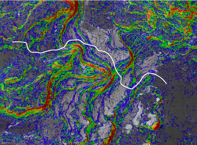
Figure 1: Mars surface (Eberswalde Crater) slope uncertainty for rover navigation: the slopes range within (blue) $5^{\circ}-10^{\circ}$, (green) $10^{\circ}-15^{\circ}$, (yellow) $15^{\circ}-20^{\circ}$, (orange) $20^{\circ}-25^{\circ}$, (red) $\geq 25^{\circ}$, and (the rest) $<5^{\circ}$ or no data.

Risk can be quantified in numerous ways, such as chance constraints (Ono et al. 2015; Wang, Jasour, and Williams 2020). However, applications in autonomy and robotics require more “nuanced assessments of risk” (Majumdar and Pavone 2020). Artzner et. al. (Artzner et al. 1999) characterized a set of natural properties that are desirable for a risk measure, called a coherent risk measure, and have obtained widespread acceptance in finance and operations research, among other fields. An important example of a coherent risk measure is the conditional value-at-risk (CVaR) that has received significant attention in decision making problems, such as Markov decision processes (MDPs) (Chow et al. 2015; Chow and Ghavamzadeh 2014; Prashanth 2014; Bäuerle and Ott 2011).

In many real world applications, risk-averse decision making should account for system constraints, such as fuel budget, communication rates, and etc. In this paper, we attempt to address this issue and therefore consider MDPs with both total coherent risk costs and constraints. Using a Lagrangian framework and properties of coherent risk measures, we propose an optimization problem, whose solution provides a lower bound to the constrained risk-averse MDP problem. We show that this result is indeed a generalization of constrained MDPs with total expected cost costs and constraints (Altman 1999). For general coherent risk measures, we show that this optimization problem is a difference convex program (DCP) and propose a method based on disciplined convex-concave programming to solve it. We illustrate our proposed method with a numerical example of path planning under uncertainty with not only CVaR risk measure but also the more recently proposed entropic value-at-risk (EVaR) (Ahmadi-Javid 2012; McAllister et al. 2020) coherent risk measure.

Notation: We denote by $\mathbb{R}^{n}$ the $n$-dimensional Euclidean space and $\mathbb{N}_{\geq 0}$ the set of non-negative integers. Throughout the paper, we use bold font to denote a vector and $(\cdot)^{\top}$ for its transpose, e.g., $\boldsymbol{a}=(a_{1},\ldots,a_{n})^{\top}$, with $n\in\{1,2,\ldots\}$. For a vector $\boldsymbol{a}$, we use $\boldsymbol{a}\succeq(\preceq)\boldsymbol{0}$ to denote element-wise non-negativity (non-positivity) and $\boldsymbol{a}\equiv\boldsymbol{0}$ to show all elements of $\boldsymbol{a}$ are zero. For two vectors $a,b\in\mathbb{R}^{n}$, we denote their inner product by $\langle\boldsymbol{a},\boldsymbol{b}\rangle$, i.e., $\langle\boldsymbol{a},\boldsymbol{b}\rangle=\boldsymbol{a}^{\top}\boldsymbol{b}$. For a finite set $\mathcal{A}$, we denote its power set by $2^{\mathcal{A}}$, i.e., the set of all subsets of $\mathcal{A}$. For a probability space $(\Omega,\mathcal{F},\mathbb{P})$ and a constant $p\in[1,\infty)$, $\mathcal{L}_{p}(\Omega,\mathcal{F},\mathbb{P})$ denotes the vector space of real valued random variables $c$ for which $\mathbb{E}|c|^{p}<\infty$.

Preliminaries

In this section, we briefly review some notions and definitions used throughout the paper.

Markov Decision Processes

An MDP is a tuple $\mathcal{M}=(\mathcal{S},Act,T,\kappa_{0})$ consisting of a set of states $\mathcal{S}=\{s_{1},\dots,s_{|\mathcal{S}|}\}$ of the autonomous agent(s) and world model, actions $Act=\{\alpha_{1},\dots,\alpha_{|Act|}\}$ available to the robot, a transition function $T(s_{j}|s_{i},\alpha)$, and $\kappa_{0}$ describing the initial distribution over the states.

This paper considers finite Markov decision processes, where $\mathcal{S}$, and $Act$ are finite sets. For each action the probability of making a transition from state $s_{i}\in\mathcal{S}$ to state $s_{j}\in\mathcal{S}$ under action $\alpha\in Act$ is given by $T(s_{j}|s_{i},\alpha)$.

The probabilistic components of a Markov decision process must satisfy the following:

$$\begin{cases}\sum_{s\in\mathcal{S}}T(s|s_{i},\alpha)=1,&\forall s_{i}\in\mathcal{S},\alpha\in Act,\\ \sum_{s\in\mathcal{S}}\kappa_{0}(s)=1.&{}\textstyle\end{cases}$$

Coherent Risk Measures

Consider a probability space $(\Omega,\mathcal{F},\mathbb{P})$, a filteration $\mathcal{F}_{0}\subset\cdots\mathcal{F}_{N}\subset\mathcal{F}$, and an adapted sequence of random variables (stage-wise costs) $c_{t},\leavevmode\nobreak\ t=0,\ldots,N$, where $N\in\mathbb{N}_{\geq 0}\cup\{\infty\}$. For $t=0,\ldots,N$, we further define the spaces $\mathcal{C}_{t}=\mathcal{L}_{p}(\Omega,\mathcal{F}_{t},\mathbb{P})$, $p\in[0,\infty)$, $\mathcal{C}_{t:N}=\mathcal{C}_{t}\times\cdots\times\mathcal{C}_{N}$ and $\mathcal{C}=\mathcal{C}_{0}\times\mathcal{C}_{1}\times\cdots$. We assume that the sequence $\boldsymbol{c}\in\mathcal{C}$ is almost surely bounded (with exceptions having probability zero), i.e., $\max_{t}\operatorname*{ess\,sup}\leavevmode\nobreak\ |c_{t}(\omega)|<\infty.$

In order to describe how one can evaluate the risk of sub-sequence $c_{t},\ldots,c_{N}$ from the perspective of stage $t$, we require the following definitions.

Definition 1 (Conditional Risk Measure).

A mapping $\rho_{t:N}:\mathcal{C}_{t:N}\to\mathcal{C}_{t}$, where $0\leq t\leq N$, is called a conditional risk measure, if it has the following monoticity property:

$$\rho_{t:N}(\boldsymbol{c})\leq\rho_{t:N}(\boldsymbol{c}^{\prime}),\quad\forall\boldsymbol{c},\forall\boldsymbol{c}^{\prime}\in\mathcal{C}_{t:N}\leavevmode\nobreak\ \text{such that}\leavevmode\nobreak\ \boldsymbol{c}\preceq\boldsymbol{c}^{\prime}.$$

Definition 2 (Dynamic Risk Measure).

A dynamic risk measure is a sequence of conditional risk measures $\rho_{t:N}:\mathcal{C}_{t:N}\to\mathcal{C}_{t}$, $t=0,\ldots,N$.

One fundamental property of dynamic risk measures is their consistency over time (Ruszczyński 2010, Definition 3). That is, if $c$ will be as good as $c^{\prime}$ from the perspective of some future time $\theta$, and they are identical between time $\tau$ and $\theta$, then $c$ should not be worse than $c^{\prime}$ from the perspective at time $\tau$. If a risk measure is time-consistent, we can define the one-step conditional risk measure $\rho_{t}:\mathcal{C}_{t+1}\to\mathcal{C}_{t}$, $t=0,\ldots,N-1$ as follows:

$$\rho_{t}(c_{t+1})=\rho_{t,t+1}(0,c_{t+1}),$$ (1)

and for all $t=1,\ldots,N$, we obtain:

$$\rho_{t,N}(c_{t},\ldots,c_{N})=\rho_{t}\big{(}c_{t}+\rho_{t+1}(c_{t+1}+\rho_{t+2}(c_{t+2}+\cdots\\ +\rho_{N-1}\left(c_{N-1}+\rho_{N}(c_{N})\right)\cdots))\big{)}.$$ (2)

Note that the time-consistent risk measure is completely defined by one-step conditional risk measures $\rho_{t}$, $t=0,\ldots,N-1$ and, in particular, for $t=0$, (2) defines a risk measure of the entire sequence $\boldsymbol{c}\in\mathcal{C}_{0:N}$.

At this point, we are ready to define a coherent risk measure.

Definition 3 (Coherent Risk Measure).

We call the one-step conditional risk measures $\rho_{t}:\mathcal{C}_{t+1}\to\mathcal{C}_{t}$, $t=1,\ldots,N-1$ as in (2) a coherent risk measure if it satisfies the following conditions

• Convexity: $\rho_{t}(\lambda c+(1-\lambda)c^{\prime})\leq\lambda\rho_{t}(c)+(1-\lambda)\rho_{t}(c^{\prime})$, for all $\lambda\in(0,1)$ and all $c,c^{\prime}\in\mathcal{C}_{t+1}$;

• Monotonicity: If $c\leq c^{\prime}$ then $\rho_{t}(c)\leq\rho_{t}(c^{\prime})$ for all $c,c^{\prime}\in\mathcal{C}_{t+1}$;

• Translational Invariance: $\rho_{t}(c+c^{\prime})=c+\rho_{t}(c^{\prime})$ for all $c\in\mathcal{C}_{t}$ and $c^{\prime}\in\mathcal{C}_{t+1}$;

• Positive Homogeneity: $\rho_{t}(\beta c)=\beta\rho_{t}(c)$ for all $c\in\mathcal{C}_{t+1}$ and $\beta\geq 0$.

Henceforth, all the risk measures considered are assumed to be coherent. In this paper, we are interested in the discounted infinite horizon problems. Let $\gamma\in(0,1)$ be a given discount factor. For $N=0,1,\ldots$, we define the functionals

$$\rho^{\gamma}_{0,t}(c_{0},\ldots,c_{t})=\rho_{0,t}(c_{0},\gamma c_{1},\ldots,\gamma^{t}c_{t})\\ =\rho_{0}\bigg{(}c_{0}+\rho_{1}\big{(}\gamma c_{1}+\rho_{2}(\gamma^{2}c_{2}+\cdots\\ \leavevmode\nobreak\ \leavevmode\nobreak\ +\rho_{t-1}\left(\gamma^{t-1}c_{t-1}+\rho_{N}(\gamma^{t}c_{t})\right)\cdots)\big{)}\bigg{)},$$ (3)

which are the same as (2) for $t=0$, but with discounting $\gamma^{t}$ applied to each $c_{t}$. Finally, we have total discounted risk functional $\rho^{\gamma}:\mathcal{C}\to\mathbb{R}$ defined as

$$\rho^{\gamma}(\boldsymbol{c})=\lim_{t\to\infty}\rho^{\gamma}_{0,t}(c_{0},\ldots,c_{t}).$$ (4)

From (Ruszczyński 2010, Theorem 3), we have that $\rho^{\gamma}$ is convex, monotone, and positive homogeneous.

Constrained Risk-Averse MDPs

Notions of coherent risk and dynamic risk measures discussed in the previous section have been developed and applied in microeconomics and mathematical finance fields in the past two decades (Vose 2008). Generally, risk-averse decision making is concerned with the behavior of agents, e.g. consumers and investors, who, when exposed to uncertainty, attempt to lower that uncertainty. The agents avoid situations with unknown payoffs, in favor of situations with payoffs that are more predictable, even if they are lower.

In a Markov decision making setting, the main idea in risk-averse control is to replace the conventional risk-neutral conditional expectation of the cumulative cost objectives with the more general coherent risk measures. In a path planning setting, we will show in our numerical experiments that considering coherent risk measures will lead to significantly more robustness to environment uncertainty.

In addition to risk-aversity, an autonomous agent is often subject to constraints, e.g. fuel, communication, or energy budgets. These constraints can also represent mission objectives, e.g. explore an area or reach a goal.

Consider a stationary controlled Markov process $\{s_{t}\}$, $t=0,1,\ldots$, wherein policies, transition probabilities, and cost functions do not depend explicitly on time. Each policy $\pi=\{\pi_{t}\}_{t=0}^{\infty}$ leads to cost sequences $\boldsymbol{c}_{t}=c(s_{t},\alpha_{t})$, $t=0,1,\ldots$ and $\boldsymbol{d}_{t}^{i}=d^{i}(s_{t},\alpha_{t})$, $t=0,1,\ldots$, $i=1,2,\ldots,n_{c}$. We define the dynamic risk of evaluating the $\gamma$-discounted cost of a policy $\pi$ as

$$J_{\gamma}(\kappa_{0},\pi)=\rho^{\gamma}\big{(}c(s_{0},\alpha_{0}),c(s_{1},\alpha_{1}),\ldots\big{)},$$ (5)

and the $\gamma$-discounted dynamic risk constraints of executing policy $\pi$ as

$$D_{\gamma}^{i}(\kappa_{0},\pi)=\rho^{\gamma}\left(d^{i}(s_{0},\alpha_{0}),d^{i}(s_{1},\alpha_{1}),\ldots\right)\leq\beta^{i},\\ i=1,2,\ldots,n_{c},$$ (6)

where $\rho^{\gamma}$ is defined in equation (4), $s_{0}\sim\kappa_{0}$, and $\beta^{i}>0$, $i=1,2,\ldots,n_{c}$, are given constants.

In this work, we are interested in addressing the following problem:

Problem 1.

For a given Markov decision process, a discount factor $\gamma\in(0,1)$, and a total risk functional $J_{\gamma}(\kappa_{0},\pi)$ as in equation (5) and total cost constraints (6) with $\{\rho_{t}\}_{t=0}^{\infty}$ being coherent risk measures, compute

$$\pi^{*}\in \leavevmode\nobreak\ \operatorname*{argmin}_{\pi}\leavevmode\nobreak\ \leavevmode\nobreak\ J_{\gamma}(\kappa_{0},\pi)$$

$$\text{subject to}\quad\boldsymbol{D}_{\gamma}(\kappa_{0},\pi)\preceq\boldsymbol{\beta}.$$ (7)

We call a controlled Markov process with the “nested” objective (5) and constraints (6) a constrained risk-averse MDP. It was previously demonstrated in (Chow et al. 2015; Osogami 2012) that such coherent risk measure objectives can account for modeling errors and parametric uncertainty in MDPs. One interpretation for Problem 1 is that we are interested in policies that minimize the incurred costs in the worst-case in a probabilistic sense and at the same time ensure that the system constraints, e.g., fuel constraints, are not violated even in the worst-case probabilistic scenarios.

Note that in Problem 1 both the objective function and the constraints are in general non-differentiable and non-convex in policy $\pi$ (with the exception of total expected cost as the coherent risk measure $\rho^{\gamma}$ (Altman 1999)). Therefore, finding optimal policies in general may be hopeless. Instead, we find sub-optimal polices by taking advantage of a Lagrangian formulation and then using an optimization form of Bellman’s equations.

Next, we show that the constrained risk-averse problem is equivalent to a non-constrained inf-sup risk-averse problem thanks to the Lagrangian method.

Proposition 1.

Let $J_{\gamma}(\kappa_{0})$ be the value of Problem 1 for a given initial distribution $\kappa_{0}$ and discount factor $\gamma$. Then, (i) the value function satisfies

$$J_{\gamma}(\kappa_{0})=\inf_{\pi}\sup_{\boldsymbol{\lambda}\succeq\boldsymbol{0}}L_{\gamma}(\pi,{\boldsymbol{\lambda}}),$$ (8)

where

$$L_{\gamma}(\pi,\boldsymbol{\lambda})=J_{\gamma}(\kappa_{0},\pi)+\langle\boldsymbol{\lambda},\left(\boldsymbol{D}_{\gamma}(\kappa_{0},\pi)-\boldsymbol{\beta}\right)\rangle,$$ (9)

is the Lagrangian function.
(ii) Furthermore, a policy $\pi^{*}$ is optimal for Problem 1, if and only if $J_{\gamma}(\kappa_{0})=\sup_{\boldsymbol{\lambda}\succeq\boldsymbol{0}}\leavevmode\nobreak\ L_{\gamma}(\pi^{*},\boldsymbol{\lambda})$.

At any time $t$, the value of $\rho_{t}$ is $\mathcal{F}_{t}$-measurable and is allowed to depend on the entire history of the process $\{s_{0},s_{1},\ldots\}$ and we cannot expect to obtain a Markov optimal policy (Ott 2010). In order to obtain Markov policies, we need the following property (Ruszczyński 2010).

Definition 4.

Let $m,n\in[1,\infty)$ such that $1/m+1/n=1$ and

$$\mathcal{P}=\big{\{}p\in\mathcal{L}_{n}(\mathcal{S},2^{\mathcal{S}},\mathbb{P})\mid\sum_{s^{\prime}\in\mathcal{S}}p(s^{\prime})\mathbb{P}(s^{\prime})=1,\leavevmode\nobreak\ p\geq 0\big{\}}.$$

A one-step conditional risk measure $\rho_{t}:\mathcal{C}_{t+1}\to\mathcal{C}_{t}$ is a Markov risk measure with respect to the controlled Markov process $\{s_{t}\}$, $t=0,1,\ldots$, if there exist a risk transition mapping $\sigma_{t}:\mathcal{L}_{m}(\mathcal{S},2^{\mathcal{S}},\mathbb{P})\times\mathcal{S}\times\mathcal{P}\to\mathbb{R}$ such that for all $v\in\mathcal{L}_{m}(\mathcal{S},2^{\mathcal{S}},\mathbb{P})$ and $\alpha_{t}\in\pi(s_{t})$, we have

$$\rho_{t}(v(s_{t+1}))=\sigma_{t}(v(s_{t+1}),s_{t},p(s_{t+1}|s_{t},\alpha_{t})),$$ (10)

where $p:\mathcal{S}\times Act\to\mathcal{P}$ is called the controlled kernel.

In fact, if $\rho_{t}$ is a coherent risk measure, $\sigma_{t}$ also satisfies the properties of a coherent risk measure (Definition 3). In this paper, since we are concerned with MDPs, the controlled kernel is simply the transition function $T$.

Assumption 1.

The one-step coherent risk measure $\rho_{t}$ is a Markov risk measure.

The simplest case of the risk transition mapping is in the conditional expectation case $\rho_{t}(v(s_{t+1}))=\mathbb{E}\{v(s_{t+1})\mid s_{t},\alpha_{t}\}$, i.e.,

$$\sigma\left\{v(s_{t+1}),s_{t},p(s_{t+1}|s_{t},\alpha_{t})\right\}=\mathbb{E}\{v(s_{t+1})\mid s_{t},\alpha_{t}\}\\ =\sum_{s_{t+1}\in\mathcal{S}}v(s_{t+1})T(s_{t+1}\mid s_{t},\alpha_{t}).$$ (11)

Note that in the total discounted expectation case $\sigma$ is a linear function in $v$ rather than a convex function, which is the case for a general coherent risk measures. In the next result, we show that we can find a lower bound to the solution to Problem 1 via solving an optimization problem.

Theorem 1.

Consider an MDP $\mathcal{M}$ with the nested risk objective (5), constraints (6), and discount factor $\gamma\in(0,1)$. Let Assumption 1 hold, let $\rho_{t},\leavevmode\nobreak\ t=0,1,\ldots$ be coherent risk measures as described in Definition 3, and suppose $c(\cdot,\cdot)$ and $d^{i}(\cdot,\cdot)$, $i=1,2,\ldots,n_{c}$, be non-negative and upper-bounded. Then, the solution $(\boldsymbol{V}^{*}_{\gamma},\boldsymbol{\lambda}^{*})$ to the following optimization problem (Bellman’s equation)

$$\sup_{\boldsymbol{V}_{\gamma},\boldsymbol{\lambda}\succeq\boldsymbol{0}}\leavevmode\nobreak\ \leavevmode\nobreak\ \langle\boldsymbol{\kappa_{0}},\boldsymbol{V}_{\gamma}\rangle-\langle\boldsymbol{\lambda},\boldsymbol{\beta}\rangle$$

subject to

$$V_{\gamma}(s)\leq c(s,\alpha)+\langle\boldsymbol{\lambda},\boldsymbol{d}(s,\alpha)\rangle$$

$$\quad\quad\quad+\gamma\sigma\{{V}_{\gamma}(s^{\prime}),s,p(s^{\prime}|s,\alpha)\},\leavevmode\nobreak\ \forall s\in\mathcal{S},\leavevmode\nobreak\ \forall\alpha\in{Act,}$$ (12)

satisfies

$$J_{\gamma}(\kappa_{0})\geq\langle\boldsymbol{\kappa_{0}},\boldsymbol{V}^{*}_{\gamma}\rangle-\langle\boldsymbol{\lambda}^{*},\boldsymbol{\beta}\rangle.$$ (13)

One interesting observation is that if the coherent risk measure $\rho^{t}$ is the total discounted expectation, then Theorem 1 is consistent with the result by (Altman 1999).

Corollary 1.

Let the assumptions of Theorem 1 hold and let $\rho_{t}(\cdot)=\mathbb{E}(\cdot|s_{t},\alpha_{t})$, $t=1,2,\ldots$. Then the solution $(\boldsymbol{V}^{*}_{\gamma},\boldsymbol{\lambda}^{*})$ to optimization (1) satisfies

$$J_{\gamma}(\kappa_{0})=\langle\boldsymbol{\kappa_{0}},\boldsymbol{V}^{*}_{\gamma}\rangle-\langle\boldsymbol{\lambda}^{*},\boldsymbol{\beta}\rangle.$$

Furthermore, with $\rho_{t}(\cdot)=\mathbb{E}(\cdot|s_{t},\alpha_{t})$, $t=1,2,\ldots$, optimization (1) becomes a linear program.

Once the values of $\boldsymbol{\lambda}^{*}$ and $\boldsymbol{V}^{*}_{\gamma}$ are found by solving optimization problem (1), we can find the policy as

$$\pi^{*}(s)\in \leavevmode\nobreak\ \operatorname*{argmin}_{\alpha\in Act}\leavevmode\nobreak\ \Big{(}c(s,\alpha)+\langle\boldsymbol{\lambda}^{*},\boldsymbol{d}(s,\alpha)\rangle$$

$$\quad\quad\quad\quad+\gamma\sigma\{V^{*}_{\gamma}(s^{\prime}),s,p(s^{\prime}|s,\alpha)\}\Big{)}.$$ (14)

Note that $\pi^{*}$ is a deterministic, stationary policy. Such policies are desirable in practical applications, since they are more convenient to implement on actual robots. Given an uncertain environment, $\pi^{*}$ can be designed offline and used for path planning.

In the next section, we discuss methods to find solutions to optimization problem (1), when $\rho^{\gamma}$ is an arbitrary coherent risk measure.

DCPs for Constrained Risk-Averse MDPs

Note that since $\rho^{\gamma}$ is a coherent, Markov risk measure (Assumption 1), $v\mapsto\sigma(v,\cdot,\cdot)$ is convex (because $\sigma$ is also a coherent risk measure). Next, we demonstrate that optimization problem (1) is indeed a DCP. Re-formulating equation (1) as a minimization yields

$$\inf_{\boldsymbol{V}_{\gamma},\boldsymbol{\lambda}\succeq\boldsymbol{0}}\leavevmode\nobreak\ \leavevmode\nobreak\ \langle\boldsymbol{\lambda},\boldsymbol{\beta}\rangle-\langle\boldsymbol{\kappa_{0}},\boldsymbol{V}_{\gamma}\rangle$$

subject to

$$V_{\gamma}(s)\leq c(s,\alpha)+\langle\boldsymbol{\lambda},\boldsymbol{d}(s,\alpha)\rangle$$

$$\quad\quad\quad+\gamma\sigma\{{V}_{\gamma}(s^{\prime}),s,p(s^{\prime}|s,\alpha)\},\leavevmode\nobreak\ \forall s\in\mathcal{S},\leavevmode\nobreak\ \forall\alpha\in{Act}.$$ (15)

At this point, we define $f_{0}(\boldsymbol{\lambda})=\langle\boldsymbol{\lambda},\boldsymbol{\beta}\rangle$, $g_{0}(\boldsymbol{V}_{\gamma})=\langle\boldsymbol{\kappa_{0}},\boldsymbol{V}_{\gamma}\rangle$, $f_{1}({V}_{\gamma})={V}_{\gamma}$, $g_{1}(\boldsymbol{\lambda})=c+\langle\boldsymbol{\lambda},\boldsymbol{d}\rangle$, and $g_{2}({V}_{\gamma})=\gamma\sigma(V_{\gamma},\cdot,\cdot)$. Note that $f_{0}$ and $g_{1}$ are convex (linear) functions of $\boldsymbol{\lambda}$ and $g_{0}$, $f_{1}$, and $g_{2}$ are convex functions in $\boldsymbol{V}_{\gamma}$. Then, we can re-write (DCPs for Constrained Risk-Averse MDPs) as

$$\inf_{\boldsymbol{V}_{\gamma},\boldsymbol{\lambda}\succeq\boldsymbol{0}}\leavevmode\nobreak\ \leavevmode\nobreak\ f_{0}(\boldsymbol{\lambda})-g_{0}(\boldsymbol{V}_{\gamma})$$

subject to

$$f_{1}({V}_{\gamma})-g_{1}(\boldsymbol{\lambda})-g_{2}({V}_{\gamma})\leq 0,\leavevmode\nobreak\ \leavevmode\nobreak\ \forall s,\alpha.$$ (16)

In fact, optimization problem (DCPs for Constrained Risk-Averse MDPs) is a standard DCP (Horst and Thoai 1999). DCPs arise in many applications, such as feature selection in machine learning (Le Thi et al. 2008) and inverse covariance estimation in statistics (Thai et al. 2014). Although DCPs can be solved globally (Horst and Thoai 1999), e.g. using branch and bound algorithms (Lawler and Wood 1966), a locally optimal solution can be obtained based on techniques of nonlinear optimization (Bertsekas 1999) more efficiently. In particular, in this work, we use a variant of the convex-concave procedure (Lipp and Boyd 2016; Shen et al. 2016), wherein the concave terms are replaced by a convex upper bound and solved. In fact, the disciplined convex-concave programming (DCCP) (Shen et al. 2016) technique linearizes DCP problems into a (disciplined) convex program (carried out automatically via the DCCP Python package (Shen et al. 2016)), which is then converted into an equivalent cone program by replacing each function with its graph implementation. Then, the cone program can be solved readily by available convex programming solvers, such as CVXPY (Diamond and Boyd 2016).

At this point, we should point out that solving (1) via the DCCP method, finds the (local) saddle points to optimization problem  (1). However, from Theorem 1, we have that every saddle point to (1) satisfies (13). In other words, every saddle point corresponds to a lower bound to the optimal value of Problem 1.

DCPs for CVaR and EVaR Risk Measures

In this section, we present the specific DCPs for finding the risk value functions for two coherent risk measures studied in our numerical experiments, namely, CVaR and EVaR.

For a given confidence level $\varepsilon\in(0,1)$, value-at-risk ($\mathrm{VaR}_{\varepsilon}$) denotes the $(1-\varepsilon)$-quantile value of the cost variable. $\mathrm{CVaR}_{\varepsilon}$ measures the expected loss in the $(1-\varepsilon)$-tail given that the particular threshold $\mathrm{VaR}_{\varepsilon}$ has been crossed. $\mathrm{CVaR}_{\varepsilon}$ is given by

$$\rho_{t}(c_{t+1})=\inf_{\zeta\in\mathbb{R}}\left\{\zeta+\frac{1}{\varepsilon}\mathbb{E}\left[(c_{t+1}-\zeta)_{+}\mid\mathcal{F}_{t}\right]\right\},$$ (17)

where $(\cdot)_{+}=\max\{\cdot,0\}$. A value of $\varepsilon\simeq 1$ corresponds to a risk-neutral policy; whereas, a value of $\varepsilon\to 0$ is rather a risk-averse policy.

In fact, Theorem 1 can applied to CVaR since it is a coherent risk measure. For an MDP $\mathcal{M}$, the risk value functions can be computed by DCP (DCPs for Constrained Risk-Averse MDPs), where

$$g_{2}({V}_{\gamma})=\inf_{\zeta\in\mathbb{R}}\left\{\zeta+\frac{1}{\varepsilon}\sum_{s^{\prime}\in\mathcal{S}}\left(V_{\gamma}(s^{\prime})-\zeta\right)_{+}T(s^{\prime}\mid s,\alpha)\right\},$$

where the infimum on the right hand side of the above equation can be absorbed into the overal infimum problem, i.e., $\inf_{\boldsymbol{V}_{\gamma},\boldsymbol{\lambda}\succeq\boldsymbol{0},\zeta}$. Note that $g_{2}({V}_{\gamma})$ above is convex in $\zeta$ (Rockafellar, Uryasev et al. 2000, Theorem 1) because the function $(\cdot)_{+}$ is increasing and convex (Ott 2010, Lemma A.1., p. 117).

Unfortunately, CVaR ignores the losses below the VaR threshold. EVaR is the tightest upper bound in the sense of Chernoff inequality for the value at risk (VaR) and CVaR and its dual representation is associated with the relative entropy. In fact, it was shown in (Ahmadi-Javid and Pichler 2017) that $\mathrm{EVaR}_{\varepsilon}$ and $\mathrm{CVaR}_{\varepsilon}$ are equal only if there are no losses ($c\to-\infty$) below the $\mathrm{VaR}_{\varepsilon}$ threshold. In addition, EVaR is a strictly monotone risk measure; whereas, CVaR is only monotone (Ahmadi-Javid and Fallah-Tafti 2019). $\mathrm{EVaR}_{\varepsilon}$ is given by

$$\rho_{t}(c_{t+1})=\inf_{\zeta>0}\left({\log\left(\frac{\mathbb{E}[e^{\zeta c_{t+1}}\mid\mathcal{F}_{t}]}{\varepsilon}\right)/\zeta}\right).$$ (18)

Similar to $\mathrm{CVaR}_{\varepsilon}$, for $\mathrm{EVaR}_{\varepsilon}$, $\varepsilon\to 1$ corresponds to a risk-neutral case; whereas, $\varepsilon\to 0$ corresponds to a risk-averse case. In fact, it was demonstrated in (Ahmadi-Javid 2012, Proposition 3.2) that $\lim_{\varepsilon\to 0}\mathrm{EVaR}_{\varepsilon}(Z)=\operatorname*{ess\,sup}(Z)$.

Since $\mathrm{EVaR}_{\varepsilon}$ is a coherent risk measure, the conditions of Theorem 1 hold. Since $\zeta>0$, using the change of variables, $\tilde{\boldsymbol{V}}_{\gamma}\equiv\zeta{\boldsymbol{V}}_{\gamma}$ and $\tilde{\boldsymbol{\lambda}}\equiv\zeta{\boldsymbol{\lambda}}$ (note that this change of variables is monotone increasing in $\zeta$ (Agrawal et al. 2018)), we can compute EVaR value functions by solving (DCPs for Constrained Risk-Averse MDPs), where

$$\begin{cases}f_{0}(\tilde{\boldsymbol{\lambda}})=\langle\tilde{\boldsymbol{\lambda}},\boldsymbol{\beta}\rangle,\\ f_{1}(\tilde{V}_{\gamma})=\tilde{V}_{\gamma},\\ g_{0}(\tilde{\boldsymbol{V}}_{\gamma})=\langle\boldsymbol{\kappa_{0}},\tilde{\boldsymbol{V}}_{\gamma}\rangle,\\ g_{1}(\tilde{\boldsymbol{\lambda}})=\zeta c+\langle\tilde{\boldsymbol{\lambda}},\boldsymbol{d}\rangle,\leavevmode\nobreak\ \text{and}\\ g_{2}(\tilde{{V}_{\gamma}})=\log\left(\frac{\sum_{s^{\prime}\in\mathcal{S}}e^{\tilde{V}_{\gamma}(s^{\prime})}T(s^{\prime}|s,\alpha)}{\varepsilon}\right).\end{cases}$$

Similar to the CVaR case, the infimum over $\zeta$ can be lumped into the overall infimum problem, i.e., $\inf_{\tilde{\boldsymbol{V}}_{\gamma},\tilde{\boldsymbol{\lambda}}\succeq\boldsymbol{0},\zeta>0}$. Note that $g_{2}(\tilde{\boldsymbol{V}}_{\gamma})$ is convex in $\tilde{V}_{\gamma}$, since the logarithm of sums of exponentials is convex (Boyd and Vandenberghe 2004, p. 72). The lower bound in (13) can then be obtained as $\frac{1}{\zeta}\left(\langle\boldsymbol{\kappa_{0}},\tilde{\boldsymbol{V}}_{\gamma}\rangle-\langle\tilde{\boldsymbol{\lambda}},\boldsymbol{\beta}\rangle\right)$.

Related Work and Discussion

We believe this work is the first study of constrained MDPs with both coherent risk objectives and constraints. We emphasize that our method leads to a policy that lower-bounds the value of Problem 1 for general coherent, Markov risk measures. In the case of no constraints $\boldsymbol{\lambda}\equiv 0$, our proposed method can also be applied to risk-averse MDPs with no constraints.

With respect to risk-averse MDPs, (Tamar et al. 2016, 2015) proposed a sampling-based algorithm for finding saddle point solutions to MDPs with total coherent risk measure costs using policy gradient methods. (Tamar et al. 2016) relies on the assumption that the risk envelope appearing in the dual representation of the coherent risk measure is known with an explicit canonical convex programming formulation. As the authors indicated, this is the case for CVaR, mean-semi-deviation, and spectral risk measures (Shapiro, Dentcheva, and Ruszczyński 2014). However, such explicit form is not known for general coherent risk measures, such as EVaR. Furthermore, it is not clear whether the saddle point solutions are a lower bound or upper bound to the optimal value. Also, policy-gradient based methods require calculating the gradient of the coherent risk measure, which is not available in explicit form in general. MDPs with CVaR constraint and total expected costs were studied in (Prashanth 2014; Chow and Ghavamzadeh 2014) and locally optimal solutions were found via policy gradients, as well. However, this method also leads to saddle point solutions and cannot be applied to general coherent risk measures. In addition, since the objective and the constraints are described by different coherent risk measures, the authors assume there exists a policy that satisfies the CVaR constraint (feasibility assumption), which may not be the case in general.

Following the footsteps of (Pflug and Pichler 2016), a promising approach based on approximate value iteration was proposed for MDPs with CVaR objectives in (Chow et al. 2015). But, it is not clear how one can extend this method to other coherent risk measures. An infinite-dimensional linear program was derived analytically for MDPs with coherent risk objectives in (Haskell and Jain 2015) with implications for solving chance and stochastic-dominance constrained MDPs. Successive finite approximation of such infinite dimensional linear programs was suggested leading to sub-optimal solutions. Yet, the method cannot be extended to constrained MDPs with coherent risk objectives and constraints. A policy iteration algorithm for finding policies that minimize total coherent risk measures for MDPs was studied in (Ruszczyński 2010; Fan and Ruszczyński 2018a) and a computational non-smooth Newton method was proposed in (Ruszczyński 2010). Our work, extends (Ruszczyński 2010; Fan and Ruszczyński 2018a) to constrained problems and uses a DCCP computational method, which takes advantage of already available software (DCCP and CVXPY).

Numerical Experiments

In this section, we evaluate the proposed methodology with a numerical example. In addition to the traditional total expectation, we consider two other coherent risk measures, namely, CVaR and EVaR. All experiments were carried out using a MacBook Pro with 2.8 GHz Quad-Core Intel Core i5 and 16 GB of RAM. The resultant linear programs and DCPs were solved using CVXPY (Diamond and Boyd 2016) with DCCP (Shen et al. 2016) add-on in Python.

Rover MDP Example Set Up

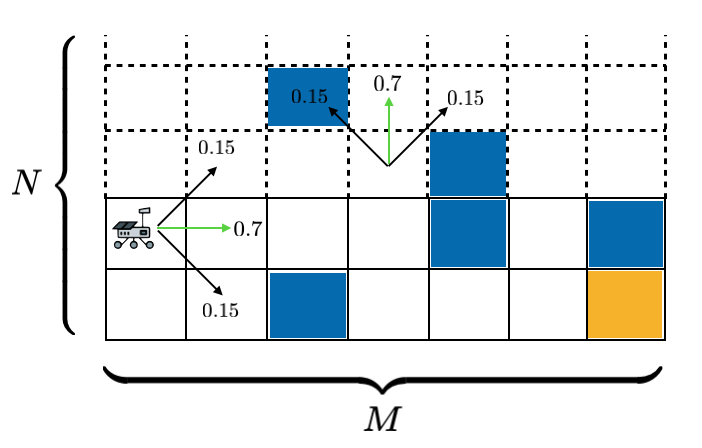
Figure 2: Grid world illustration for the rover navigation example. Blue cells denote the obstacles and the yellow cell denotes the goal.

An agent (e.g. a rover) has to autonomously navigate a two dimensional terrain map (e.g. Mars surface) represented by an $M\times N$ grid. A rover can move from cell to cell. Thus, the state space is given by $\mathcal{S}=\{s_{i}|i=x+My,x\in\{1,\dots,M\},y\in\{1,\dots,N\}\}.$ The action set available to the robot is $Act=\{E,\ W,\ N,\ S,\ NE,\ NW,\ SE,\ SW\}$, i.e., diagonal moves are allowed. The actions move the robot from its current cell to a neighboring cell, with some uncertainty. The state transition probabilities for various cell types are shown for actions $E$ and $N$ in Figure 2. Other actions lead to analogous transitions.

With regards to constraint costs, there is an stage-wise cost of each move until reaching the goal of $2$, to account for fuel usage constraints. In between the starting point and the destination, there are a number of obstacles that the agent should avoid. Hitting an obstacle incurs the immediate cost of $10$, while the goal grid region has zero immediate cost. These two latter immediate costs are captured by the cost function. The discount factor is $\gamma=0.95$.

The objective is to compute a safe path that is fuel efficient, i.e., solving Problem 1. To this end, we consider total expectation, CVaR, and EVaR as the coherent risk measure.

As a robustness test, inspired by (Chow et al. 2015), we included a set of single grid obstacles that are perturbed in a random direction to one of the neighboring grid cells with probability $0.2$ to represent uncertainty in the terrain map. For each risk measure, we run $100$ Monte Carlo simulations with the calculated policies and count failure rates, i.e., the number of times a collision has occurred during a run.

Results

In our experiments, we consider three grid-world sizes of $10\times 10$, $15\times 15$, and $20\times 20$ corresponding to $100$, $225$, and $400$ states, respectively. For each grid-world, we allocate 25% of the grid to obstacles, including 3, 6, and 9 uncertain (single-cell) obstacles for the $10\times 10$, $15\times 15$, and $20\times 20$ grids, respectively. In each case, we solve DCP (1) (linear program in the case of total expectation) with $|\mathcal{S}||Act|=MN\times 8=8MN$ constraints and $MN+2$ variables (the risk value functions $V_{\gamma}$’s, Langrangian coefficient $\lambda$, and $\zeta$ for CVaR and EVaR). In these experiments, we set $\varepsilon=0.15$ for CVaR and EVaR coherent risk measures. The fuel budget (constraint bound $\beta$) was set to 50, 10, and 200 for the $10\times 10$, $15\times 15$, and $20\times 20$ grid-worlds, respectively. The initial condition was chosen as $\kappa_{0}(s_{M})=1$, i.e., the agent starts at the right most grid at the bottom.

A summary of our numerical experiments is provided in Table 1. Note the computed values of Problem 1 satisfy $\mathbb{E}(c)\leq\mathrm{CVaR}_{\varepsilon}(c)\leq\mathrm{EVaR}_{\varepsilon}(c)$. This is in accordance with the theory that EVaR is a more conservative coherent risk measure than CVaR (Ahmadi-Javid 2012).

$(M\times N)_{\rho_{t}}$	$J_{\gamma}(\kappa_{0})$	Total Time [s]	# U.O.	F.R.
$(10\times 10)_{\mathbb{E}}$	5.10	0.7	3	9%
$(15\times 15)_{\mathbb{E}}$	7.53	1.0	6	18%
$(20\times 20)_{\mathbb{E}}$	8.98	1.6	9	21%
$(10\times 10)_{\text{CVaR}_{\varepsilon}}$	$\geq$7.76	5.4	3	1%
$(15\times 15)_{\text{CVaR}_{\varepsilon}}$	$\geq$9.22	8.3	6	3%
$(20\times 20)_{\text{CVaR}_{\varepsilon}}$	$\geq$12.76	10.5	9	5%
$(10\times 10)_{\text{EVaR}_{\varepsilon}}$	$\geq$7.99	3.2	3	0%
$(15\times 15)_{\text{EVaR}_{\varepsilon}}$	$\geq$11.04	4.9	6	0%
$(20\times 20)_{\text{EVaR}_{\varepsilon}}$	$\geq$15.28	6.6	9	2%

Table 1: Comparison between total expectation, CVaR, and EVaR coherent risk measures. $(M\times N)_{\rho_{t}}$ denotes experiments with grid-world of size $M\times N$ and one-step coherent risk measure $\rho_{t}$. $J_{\gamma}(\kappa_{0})$ is the valued of the constrained risk-averse problem (Problem 1). Total Time denotes the time taken by the CVXPY solver to solve the associated linear programs or DCPs in seconds. $\#$ U.O. denotes the number of single grid uncertain obstacles used for robustness test. F.R. denotes the failure rate out of 100 Monte Carlo simulations with the computed policy.

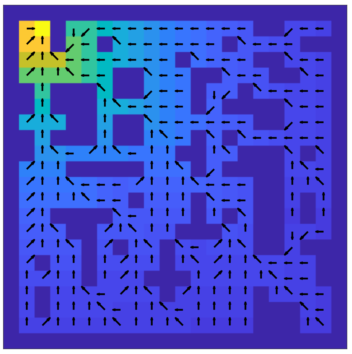
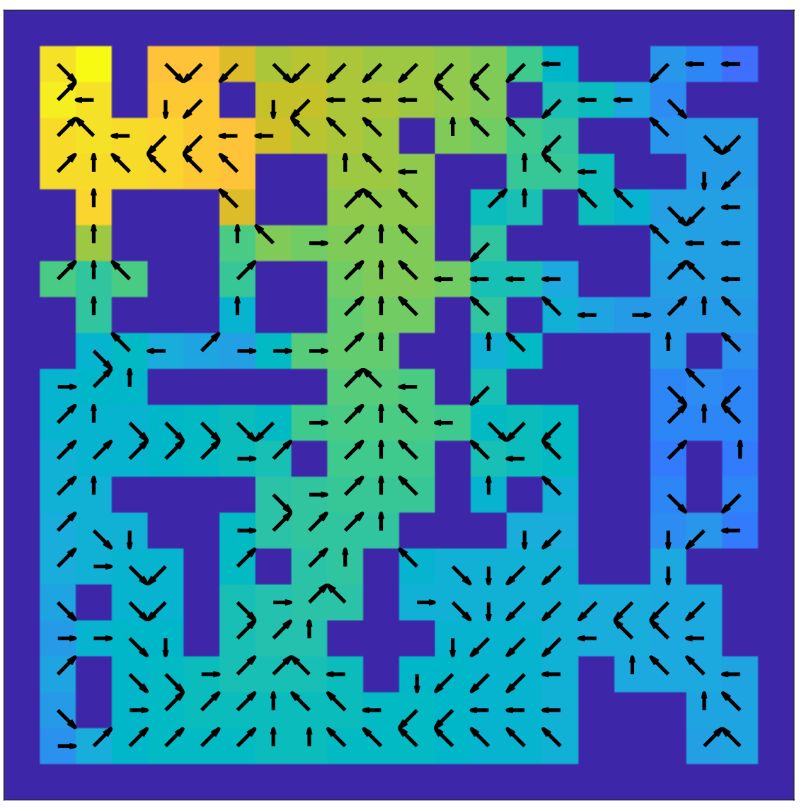
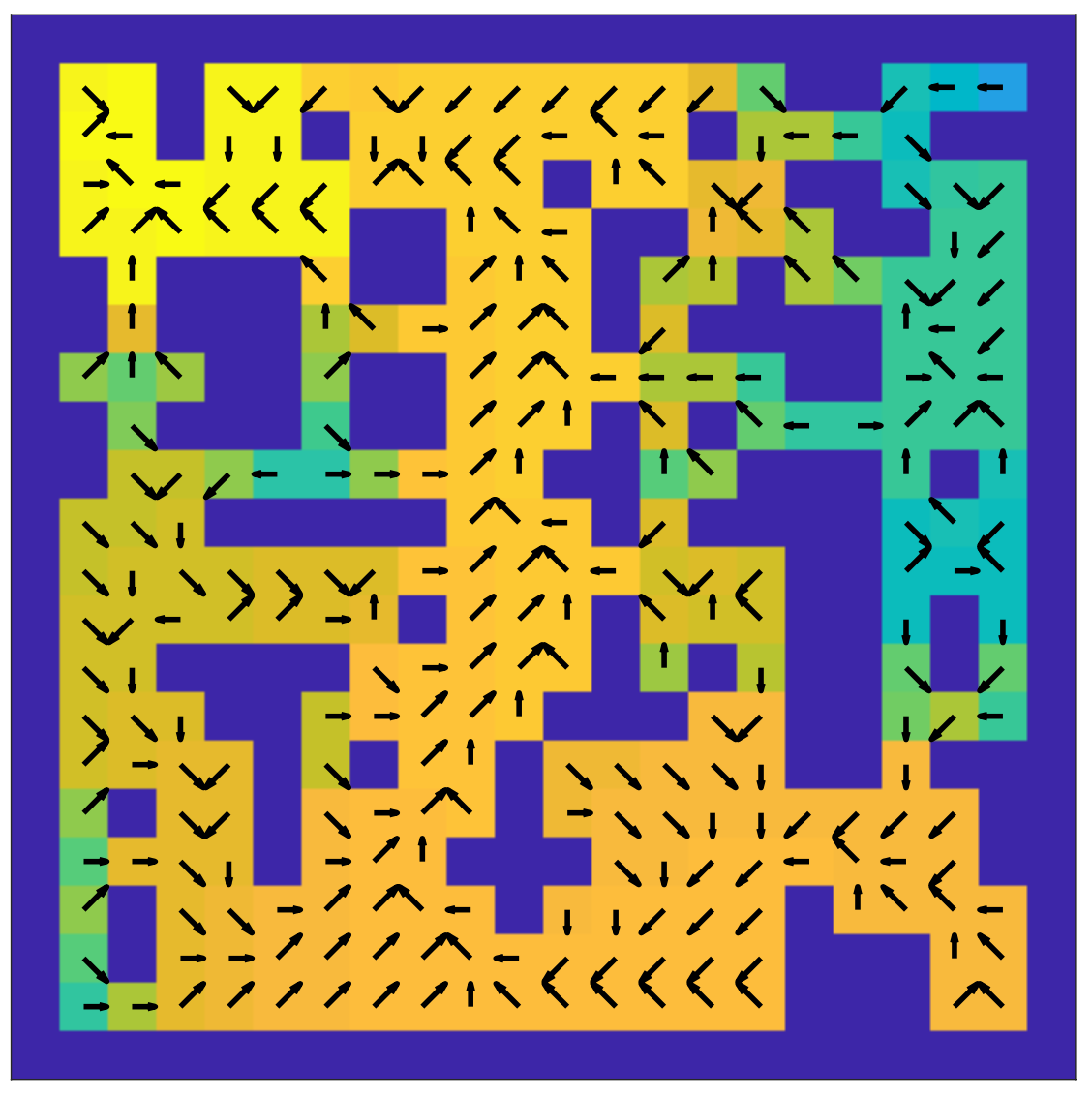
Figure 3: Results for the MDP example with total expectation (left), CVaR (middle), and EVaR (right) coherent risk measures. The goal is located at the yellow cell. Notice the 9 single cell obstacles used for robustness test.

For total expectation coherent risk measure, the calculations took significantly less time, since they are the result of solving a set of linear programs. For CVaR and EVaR, a set of DCPs were solved. CVaR calculation was the most computationally involved. This observation is consistent with (Ahmadi-Javid and Fallah-Tafti 2019) were it was discussed that EVaR calculation is much more efficient than CVaR. Note that these calculations can be carried out offline for policy synthesis and then the policy can be applied for risk-averse robot path planning.

The table also outlines the failure ratios of each risk measure. In this case, EVaR outperformed both CVaR and total expectation in terms of robustness, tallying with the fact that EVaR is conservative. In addition, these results suggest that, although discounted total expectation is a measure of performance in high number of Monte Carlo simulations, it may not be practical to use it for real-world planning under uncertainty scenarios. CVaR and especially EVaR seem to be a more reliable metric for performance in planning under uncertainty.

For the sake of illustrating the computed policies, Figure 3 depicts the results obtained from solving DCP (1) for a $20\times 20$ grid-world. The arrows on grids depict the (sub)optimal actions and the heat map indicates the values of Problem 1 for each grid state. Note that the values for EVaR are greater than those for CVaR and the values for CVaR are greater from those of total expectation. This is in accordance with the theory that $\mathbb{E}(c)\leq\mathrm{CVaR}_{\varepsilon}(c)\leq\mathrm{EVaR}_{\varepsilon}(c)$ (Ahmadi-Javid 2012). In addition, by inspecting the computed actions in obstacle dense areas of the grid-world (for example, the top right area), we infer that the actions in more risk-averse cases (especially, EVaR) have a higher tendency to steer the robot away from the obstacles given the diagonal transition uncertainty as depicted in Figure 2; whereas, for total expectation, the actions are rather concerned about taking the robot to the goal region.

Conclusions

We proposed an optimization-based method for finding sub-optimal policies that lower-bound the constrained risk-averse problem in MDPs. We showed that this optimization problem is in DCP form for general coherent risk measures and can be solved using DCCP method. Our methodology generalized constrained MDPs with total expectation risk measure to general coherent, Markov risk measures. Numerical experiments were provided to show the efficacy of our approach.

In this paper, we assumed the states are fully observable. In future work, we will consider extension of the proposed framework to Markov processes with partially observable states (Ahmadi et al. 2020; Fan and Ruszczyński 2015, 2018b). Moreover, we only considered discounted infinite horizon problems in this work. We will explore risk-averse policy synthesis in the presence of other cost criteria (Carpin, Chow, and Pavone 2016; Cavus and Ruszczynski 2014) in our prospective research. In particular, we are interested in risk-averse planning in the presence of high-level mission specifications in terms of linear temporal logic formulas (Wongpiromsarn, Topcu, and Murray 2012; Ahmadi, Sharan, and Burdick 2020).

References

- Agrawal et al. (2018) Agrawal, A.; Verschueren, R.; Diamond, S.; and Boyd, S. 2018. A rewriting system for convex optimization problems. Journal of Control and Decision 5(1): 42–60.
- Ahmadi et al. (2020) Ahmadi, M.; Ono, M.; Ingham, M. D.; Murray, R. M.; and Ames, A. D. 2020. Risk-Averse Planning Under Uncertainty. In 2020 American Control Conference (ACC), 3305–3312. IEEE.
- Ahmadi, Sharan, and Burdick (2020) Ahmadi, M.; Sharan, R.; and Burdick, J. W. 2020. Stochastic finite state control of POMDPs with LTL specifications. arXiv preprint arXiv:2001.07679 .
- Ahmadi-Javid (2012) Ahmadi-Javid, A. 2012. Entropic value-at-risk: A new coherent risk measure. Journal of Optimization Theory and Applications 155(3): 1105–1123.
- Ahmadi-Javid and Fallah-Tafti (2019) Ahmadi-Javid, A.; and Fallah-Tafti, M. 2019. Portfolio optimization with entropic value-at-risk. European Journal of Operational Research 279(1): 225–241.
- Ahmadi-Javid and Pichler (2017) Ahmadi-Javid, A.; and Pichler, A. 2017. An analytical study of norms and Banach spaces induced by the entropic value-at-risk. Mathematics and Financial Economics 11(4): 527–550.
- Altman (1999) Altman, E. 1999. Constrained Markov decision processes, volume 7. CRC Press.
- Artzner et al. (1999) Artzner, P.; Delbaen, F.; Eber, J.; and Heath, D. 1999. Coherent measures of risk. Mathematical finance 9(3): 203–228.
- Bäuerle and Ott (2011) Bäuerle, N.; and Ott, J. 2011. Markov decision processes with average-value-at-risk criteria. Mathematical Methods of Operations Research 74(3): 361–379.
- Bertsekas (1999) Bertsekas, D. 1999. Nonlinear Programming. Athena Scientific.
- Boyd and Vandenberghe (2004) Boyd, S.; and Vandenberghe, L. 2004. Convex optimization. Cambridge university press.
- Carpin, Chow, and Pavone (2016) Carpin, S.; Chow, Y.; and Pavone, M. 2016. Risk aversion in finite Markov Decision Processes using total cost criteria and average value at risk. In 2016 ieee international conference on robotics and automation (icra), 335–342. IEEE.
- Cavus and Ruszczynski (2014) Cavus, O.; and Ruszczynski, A. 2014. Risk-averse control of undiscounted transient Markov models. SIAM Journal on Control and Optimization 52(6): 3935–3966.
- Chow and Ghavamzadeh (2014) Chow, Y.; and Ghavamzadeh, M. 2014. Algorithms for CVaR optimization in MDPs. In Advances in neural information processing systems, 3509–3517.
- Chow et al. (2015) Chow, Y.; Tamar, A.; Mannor, S.; and Pavone, M. 2015. Risk-sensitive and robust decision-making: a cvar optimization approach. In Advances in Neural Information Processing Systems, 1522–1530.
- Diamond and Boyd (2016) Diamond, S.; and Boyd, S. 2016. CVXPY: A Python-embedded modeling language for convex optimization. Journal of Machine Learning Research 17(83): 1–5.
- Fan and Ruszczyński (2015) Fan, J.; and Ruszczyński, A. 2015. Dynamic risk measures for finite-state partially observable markov decision problems. In 2015 Proceedings of the Conference on Control and its Applications, 153–158. SIAM.
- Fan and Ruszczyński (2018a) Fan, J.; and Ruszczyński, A. 2018a. Process-based risk measures and risk-averse control of discrete-time systems. Mathematical Programming 1–28.
- Fan and Ruszczyński (2018b) Fan, J.; and Ruszczyński, A. 2018b. Risk measurement and risk-averse control of partially observable discrete-time Markov systems. Mathematical Methods of Operations Research 88(2): 161–184.
- Haskell and Jain (2015) Haskell, W. B.; and Jain, R. 2015. A convex analytic approach to risk-aware Markov decision processes. SIAM Journal on Control and Optimization 53(3): 1569–1598.
- Horst and Thoai (1999) Horst, R.; and Thoai, N. V. 1999. DC programming: overview. Journal of Optimization Theory and Applications 103(1): 1–43.
- Lawler and Wood (1966) Lawler, E. L.; and Wood, D. E. 1966. Branch-and-bound methods: A survey. Operations research 14(4): 699–719.
- Le Thi et al. (2008) Le Thi, H. A.; Le, H. M.; Dinh, T. P.; et al. 2008. A DC programming approach for feature selection in support vector machines learning. Advances in Data Analysis and Classification 2(3): 259–278.
- Lipp and Boyd (2016) Lipp, T.; and Boyd, S. 2016. Variations and extension of the convex–concave procedure. Optimization and Engineering 17(2): 263–287.
- Majumdar and Pavone (2020) Majumdar, A.; and Pavone, M. 2020. How should a robot assess risk? Towards an axiomatic theory of risk in robotics. In Robotics Research, 75–84. Springer.
- McAllister et al. (2020) McAllister, W.; Whitman, J.; Varghese, J.; Axelrod, A.; Davis, A.; and Chowdhary, G. 2020. Agbots 2.0: Weeding Denser Fields with Fewer Robots. Robotics: Science and Systems 2020 .
- McGhan et al. (2016) McGhan, C. L.; Vaquero, T.; Subrahmanya, A. R.; Arslan, O.; Murray, R.; Ingham, M. D.; Ono, M.; Estlin, T.; Williams, B.; and Elaasar, M. 2016. The Resilient Spacecraft Executive: An Architecture for Risk-Aware Operations in Uncertain Environments. In Aiaa Space 2016, 5541.
- Ono et al. (2018) Ono, M.; Heverly, M.; Rothrock, B.; Almeida, E.; Calef, F.; Soliman, T.; Williams, N.; Gengl, H.; Ishimatsu, T.; Nicholas, A.; et al. 2018. Mars 2020 Site-Specific Mission Performance Analysis: Part 2. Surface Traversability. In 2018 AIAA SPACE and Astronautics Forum and Exposition, 5419.
- Ono et al. (2015) Ono, M.; Pavone, M.; Kuwata, Y.; and Balaram, J. 2015. Chance-constrained dynamic programming with application to risk-aware robotic space exploration. Autonomous Robots 39(4): 555–571.
- Osogami (2012) Osogami, T. 2012. Robustness and risk-sensitivity in Markov decision processes. In Advances in Neural Information Processing Systems, 233–241.
- Ott (2010) Ott, J. T. 2010. A Markov decision model for a surveillance application and risk-sensitive Markov decision processes.
- Pflug and Pichler (2016) Pflug, G. C.; and Pichler, A. 2016. Time-consistent decisions and temporal decomposition of coherent risk functionals. Mathematics of Operations Research 41(2): 682–699.
- Prashanth (2014) Prashanth, L. 2014. Policy gradients for CVaR-constrained MDPs. In International Conference on Algorithmic Learning Theory, 155–169. Springer.
- Rockafellar, Uryasev et al. (2000) Rockafellar, R. T.; Uryasev, S.; et al. 2000. Optimization of conditional value-at-risk. Journal of risk 2: 21–42.
- Ruszczyński (2010) Ruszczyński, A. 2010. Risk-averse dynamic programming for Markov decision processes. Mathematical programming 125(2): 235–261.
- Shapiro, Dentcheva, and Ruszczyński (2014) Shapiro, A.; Dentcheva, D.; and Ruszczyński, A. 2014. Lectures on stochastic programming: modeling and theory. SIAM.
- Shen et al. (2016) Shen, X.; Diamond, S.; Gu, Y.; and Boyd, S. 2016. Disciplined convex-concave programming. In 2016 IEEE 55th Conference on Decision and Control (CDC), 1009–1014. IEEE.
- Tamar et al. (2015) Tamar, A.; Chow, Y.; Ghavamzadeh, M.; and Mannor, S. 2015. Policy gradient for coherent risk measures. In Advances in Neural Information Processing Systems, 1468–1476.
- Tamar et al. (2016) Tamar, A.; Chow, Y.; Ghavamzadeh, M.; and Mannor, S. 2016. Sequential decision making with coherent risk. IEEE Transactions on Automatic Control 62(7): 3323–3338.
- Thai et al. (2014) Thai, J.; Hunter, T.; Akametalu, A. K.; Tomlin, C. J.; and Bayen, A. M. 2014. Inverse covariance estimation from data with missing values using the concave-convex procedure. In 53rd IEEE Conference on Decision and Control, 5736–5742. IEEE.
- Vose (2008) Vose, D. 2008. Risk analysis: a quantitative guide. John Wiley & Sons.
- Wang, Jasour, and Williams (2020) Wang, A.; Jasour, A. M.; and Williams, B. 2020. Non-gaussian chance-constrained trajectory planning for autonomous vehicles under agent uncertainty. IEEE Robotics and Automation Letters .
- Wongpiromsarn, Topcu, and Murray (2012) Wongpiromsarn, T.; Topcu, U.; and Murray, R. M. 2012. Receding horizon temporal logic planning. IEEE Transactions on Automatic Control 57(11): 2817–2830.