When Does Gradient Descent with Logistic Loss
Find Interpolating Two-Layer Networks?

Abstract

We study the training of finite-width two-layer smoothed ReLU networks for binary classification using the logistic loss. We show that gradient descent drives the training loss to zero if the initial loss is small enough. When the data satisfies certain cluster and separation conditions and the network is wide enough, we show that one step of gradient descent reduces the loss sufficiently that the first result applies.

1 Introduction

The success of deep learning has led to a lot of recent interest in understanding the properties of “interpolating” neural network models, that achieve (near-)zero training loss [Zha+17, Bel+19]. One aspect of understanding these models is to theoretically characterize how first-order gradient methods (with appropriate random initialization) seem to reliably find interpolating solutions to non-convex optimization problems.

In this paper, we show that, under two sets of conditions, training fixed-width two-layer networks with gradient descent drives the logistic loss to zero. The networks have smooth “Huberized” ReLUs [Tat+20] and the output weights are not trained.

The first result only requires the assumption that the initial loss is small, but does not require any assumption about either the width of the network or the number of samples. It guarantees that if the initial loss is small then gradient descent drives the logistic loss to zero.

For our second result we assume that the inputs come from four clusters, two per class, and that the clusters corresponding to the opposite labels are appropriately separated. Under these assumptions, we show that random Gaussian initialization along with a single step of gradient descent is enough to guarantee that the loss reduces sufficiently that the first result applies.

A few proof ideas that facilitate our results are as follows: under our first set of assumptions, when the loss is small, we show that the negative gradient aligns well with the parameter vector. This yields a lower bound on the norm of the gradient in terms of the loss and the norm of the current weights. This implies that, if the weights are not too large, the loss is reduced rapidly at the beginning of the gradient descent step. Exploiting the Huberization of the ReLUs, we also show that the loss is a smooth function of the weights, so that the loss continues to decrease rapidly throughout the step, as long as the step-size is not too big. Crucially, we show that the loss is decreased significantly compared with the size of the change to the weights. This implies, in particular, that the norm of the weights does not increase by too much, so that progress can continue.

The preceding analysis requires a small loss to “get going”. Our second result provides one example when this provably happens. A two-layer network may be viewed as a weighted vote over predictions made by the hidden units. Units only vote on examples that fall in halfspaces where their activation functions are non-zero. When the network is randomly initialized, we can think of each hidden unit as “capturing” roughly half of the examples—each example is turn captured by roughly half of the hidden units. Some capturing events are helpful, and some are harmful. At initialization, these are roughly equal. Using the properties of the Gaussian initialization (including concentration and anti-concentration) we show that each example $(x_{s},y_{s})$ is captured by many nodes whose first updates contribute to improving its loss. For this to happen, the updates for this example must not be offset by updates for other examples. This happens with sufficient probability at each individual node that the cumulative effect of these “good” nodes overwhelms the effects of potentially confounding nodes, which tend to cancel one another. Consequently, with $2p$ hidden nodes, the loss after one iteration is at most $\exp(-\Omega(p^{1/2-\beta}))$ for $\beta>0$. By comparison, under similar, but weaker, clustering assumptions, [LL18] used a neural tangent kernel (NTK) analysis to show that the loss is $1/\textsf{poly}(p)$ after $\textsf{poly}(p)$ steps. Our proof uses more structure of the problem than the NTK proof, for example, that (loosely speaking) the reduction in the loss is exponential in the number of hidden units improved.

We work with smooth Huberized ReLUs to facilitate theoretical analysis. We analyze networks with Huberized ReLUs instead of the increasingly popular Swish [RZL18], which is also a smooth approximation to the ReLU, to facilitate a simple analysis. We describe some preliminary experiments with artificial data supporting our theoretical analysis, and suggesting that networks with Huberized ReLUs behave similarly to networks with standard ReLUs.

Related results, under weaker assumptions, have been obtained for the quadratic loss [Du+18, Du+19, ALS19, OS20], using the NTK [JGH18, COB19]. The logistic loss is qualitatively different; among other things, driving the logistic loss to zero requires the weights to go to infinity, far from their initial values, so that a Taylor approximation around the initial values cannot be applied. The NTK framework has also been applied to analyze training with the logistic loss. A typical result [LL18, ALS19, Zou+20] is that after $\textsf{poly}(1/\varepsilon)$ updates, a network of size/width $\textsf{poly}(1/\varepsilon)$ achieves $\varepsilon$ loss. Thus to guarantee loss very close to zero, these analyses require larger and larger networks. The reason for this appears to be that a key part of these analyses is to show that a wider network can achieve a certain fixed loss by traveling a shorter distance in parameter space. Since it seems that, to drive the logistic loss to zero with a fixed-width network, the parameters must travel an unbounded distance, the NTK approach cannot be applied to obtain the results of this paper.

In a recent paper, [LL20] studied the margin maximization of ReLU networks for the logistic loss. [LL20] also proved the convergence of gradient descent to zero, but that result requires positive homogeneity and smoothness, which rules out the ReLU and similar nonlinearities like the Huberized ReLU studied here. Their results do apply in the case that the ReLU is raised to a power strictly greater than two. Lyu and Li used both assumptions of positive homogeneity and smoothness to prove the results in their paper that are most closely related to this paper, so that a substantially different analysis was needed here. (See, for example, the proof of Lemma E.7 of their paper.) As far as we know, the analysis of the alignment between the negative gradient and the weights originated in their paper: in this paper, we establish such alignment under weaker conditions.

Building on this work by [LL20], [JT20] studied finite-width deep ReLU neural networks and showed that starting from a small loss, gradient flow coupled with logistic loss leads to convergence of the directions of the parameter vectors. They also demonstrate alignment between the parameter vector directions and the negative gradient. However, they do not prove that the training loss converges to zero.

The remainder of the paper is organized as follows. In Section 2 we introduce notation, definitions, assumptions, and present both of our main results. We provide a proof of Theorem 1 in Section 3 and we prove Theorem 2 in Section 4. Section 5 is devoted to some numerical simulations. Section 6 points to other related work and we conclude with a discussion in Section 7.

2 Preliminaries and Main Results

This section includes notational conventions, a description of the setting, and the statements of the main results.

2.1 Notation

Given a vector $v$, let $\lVert v\rVert$ denote its Euclidean norm. Given a matrix $M$, let $\lVert M\rVert$ denote its Frobenius norm and $\lVert M\rVert_{op}$ denote its operator norm. For any $k\in\mathbb{N}$, we denote the set $\{1,\ldots,k\}$ by $[k]$. For a number $d$ of inputs, we denote the set of unit-length vectors in $\mathbb{R}^{d}$ by $\mathbb{S}^{d-1}$. Given an event $A$, we let $\mathbf{1}_{A}$ denote the indicator of this event. The symbol $\wedge$ is used to denote the logical “AND" operation. At multiple points in the proof we will use the standard “big Oh notation” [Cor+09, see, e.g.,] to denote how certain quantities scale with the number of hidden units ($2p$), while viewing all other problem parameters that are not specifically set as a function of $p$ as constants. We will use $C_{1},C_{2},\ldots$ to denote absolute constants whose values are fixed throughout the paper, and $c^{\prime},c_{1},\ldots$ to denote “local” constants, which may take different values in different contexts.

2.2 The Setting

We will analyze gradient descent applied to minimize the training loss of a two-layer network.

Let $d$ be the number of inputs, and $2p$ be the number of hidden nodes. We consider the case that the weights connected to the output nodes are fixed: $p$ of them take the value $1$, and the other $p$ take the value $-1$.

We work with Huberized ReLUs that are defined as follows:

$$\phi(z):=\left\{\begin{array}[]{ll}0&\mbox{ if $z<0$,}\\ \frac{z^{2}}{2h}&\mbox{ if $z\in[0,h]$,}\\ z-h/2&\mbox{otherwise.}\end{array}\right.$$ (1)

See Figure 1.

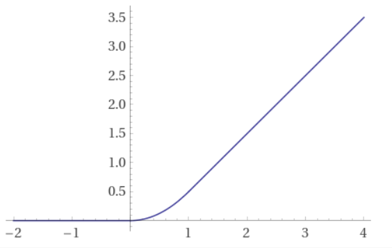
Figure 1: A plot of the Huberized ReLU in the case $h=1.$

We set the value of the bandwidth parameter $h=1/p$ throughout the paper.

For $i\in\{1,\ldots,2p\}$, let $v_{i}\in\mathbb{R}^{d}$ be vector of weights from the inputs to the $i$th hidden node, and let $u_{1},\ldots,u_{2p}\in\mathbb{R}$ be the weights connecting the hidden nodes to the output node. Set $u_{1}=\ldots=u_{p}=1$ and $u_{p+1}=\ldots=u_{2p}=-1$. Let $b_{i}$ be the bias for the $i$th hidden node. Let $\theta=(v_{1},b_{1},\ldots,v_{2p},b_{2p})$ consist of all of the trainable parameters in the network. Let $f_{\theta}$ denote the function computed by the network, which maps $x$ to

$$f_{\theta}(x)=\sum_{i=1}^{2p}u_{i}\phi(v_{i}\cdot x+b_{i}).$$

Consider a training set $(x_{1},y_{1}),\ldots,(x_{n},y_{n})\in\mathbb{S}^{d-1}\times\{-1,1\}$. Define the training loss $L$ by

$$L(\theta):=\frac{1}{n}\sum_{s=1}^{n}\log(1+\exp\left(-y_{s}f_{\theta}(x_{s})\right)),$$

and refer to loss on example $s$ by

$$L(\theta;x_{s},y_{s}):=\log(1+\exp\left(-y_{s}f_{\theta}(x_{s})\right)).$$

The gradient of the loss evaluated at $\theta$ is

$$\nabla_{\theta}L(\theta)=\frac{1}{n}\sum_{s=1}^{n}\frac{-y_{s}\nabla_{\theta}f_{\theta}(x_{s})}{1+\exp\left(y_{s}f_{\theta}(x_{s})\right)}.$$

Note that, since $\phi^{\prime\prime}$ is not defined at $0$ and $h$, the Hessian of $L$ is not defined everywhere. We use the following weak derivative of $\phi^{\prime}$ to define a weak Hessian ($\nabla^{2}_{\theta}L(\theta)$):

$$\gamma(z):=\left\{\begin{array}[]{ll}\frac{1}{h}&\mbox{ if $z\in[0,h]$,}\\ 0&\mbox{otherwise.}\end{array}\right.$$ (4)

2.3 A General Bound

We first analyze the iterates $\theta^{(1)},\theta^{(2)},\ldots$ defined by

$$\theta^{(t+1)}:=\theta^{(t)}-\alpha_{t}\nabla_{\theta}L\lvert_{\theta=\theta^{(t)}},$$

in terms of properties of $\theta^{(1)}$.

Theorem 1.

There is an absolute constant $C_{1}>0$ such that, for all $n\geq 2$, for all $p\geq 1$, for any initial parameters $\theta^{(1)}$ and dataset $(x_{1},y_{1}),\ldots,(x_{n},y_{n})\in\mathbb{S}^{d-1}\times\{-1,1\}$, for any positive $Q_{1}\leq\widetilde{Q}_{1}$ and positive $Q_{2}\leq\widetilde{Q}_{2}(Q_{1})$ (where $\widetilde{Q}_{1}$ and $\widetilde{Q}_{2}$ are defined in eqs. (8)-(9)) the following holds for all $t\geq 1$. If $h=1/p$ and each step-size $\alpha_{t}=Q_{1}\log^{2}(1/L(\theta^{(t)}))$, and if $L(\theta^{(1)})\leq\frac{1}{n^{1+C_{1}}}$ then, for all $t\geq 1$,

$$L(\theta^{(t)})\leq\frac{L(\theta^{(1)})}{Q_{2}\cdot(t-1)+1}.$$

The proof of this theorem is presented in Section 3 below.

We reiterate that this theorem makes no assumption about the number of hidden nodes ($p$) and makes a mild assumption on the number of samples required ($n\geq 2$). The only other constraint is that the initial loss needs to be smaller than $1/n^{1+C_{1}}$, for some universal constant $C_{1}>0$. Our choice of a time-varying step-size $\alpha_{t}$ that grows with $\log^{2}(1/L(\theta^{(t)}))$ leads to an upper bound on the loss that scales with $1/t$.

2.4 Clustered Data with Random Initialization

We next consider gradient descent after random initialization by showing that, after one iteration, $\theta^{(1)}$ has the favorable properties needed to apply Theorem 1. We assume that all trainable parameters are initialized by being chosen independently at random from ${\cal N}(0,\sigma^{2})$. Let $\theta^{(0)}$ be the initial value of the parameters and $\alpha_{0}$ be the original step-size (which will be chosen as a function of $p$).

This analysis depends on cluster and separation conditions. We shall use $k$ and $\ell$ to index over the clusters (ranging from $1$ to $4$), and $s$ and $q$ to index over individual samples (ranging from $1$ to $n$). We assume that the training data can be divided into four clusters ${\cal K}_{1},\ldots,{\cal K}_{4}$. All examples $(x_{s},y_{s})$ in clusters ${\cal K}_{1}$ and ${\cal K}_{2}$ have $y_{s}=1$ and all examples $(x_{s},y_{s})$ in clusters ${\cal K}_{3}$ and ${\cal K}_{4}$ have $y_{s}=-1$. For some cluster index $k$, let $y_{k}$ be the label shared by all examples in cluster ${\cal K}_{k}$. With some abuse of notation we will often use $s\in{\cal K}_{k}$ to denote that the example $(x_{s},y_{s})$ belongs to the cluster ${\cal K}_{k}$.

We make the following assumptions about the clustered training data.

• For $\varepsilon>0$, for each cluster ${\cal K}_{k}$, we assume $n_{k}:=|{\cal K}_{k}|$ satisfies $\left(1/4-\varepsilon\right)n\leq n_{k}\leq\left(1/4+\varepsilon\right)n.$

• Assume that $\lVert x_{s}\rVert=1$ for all $s\in[n]$.

• For a radius $r>0$, each cluster ${\cal K}_{k}$ has a center $\mu_{k}$ with $\lVert\mu_{k}\rVert=1$, such that for all $s\in{\cal K}_{k}$, $\lVert x_{s}-\mu_{k}\rVert\leq r$.

• For a separation parameter $\Delta>0$, we assume that for all $k,\ell$ with $y_{k}\neq y_{\ell}$, $\mu_{k}\cdot\mu_{\ell}\leq\Delta$.

Under these assumptions we demonstrate that with high probability random initialization followed by one step of gradient descent leads to a network whose training loss is at most $\exp\left(-\Omega(p^{1/2-\beta})\right)$ for $\beta>0$. Theorem 1 then implies that gradient descent in the subsequent steps leads to a solution with training loss approaching zero.

Theorem 2.

For any $\beta\in(0,1/2)$, there are absolute constants $C_{2},\ldots,C_{6}>0$ such that, under the assumptions described above, the following holds for all $\delta<1/2$ and $n\geq 4$. If $\Delta<C_{2}$, $r<C_{2}$, $\varepsilon<C_{2}$, $\alpha_{0}=\frac{1}{p^{1/2+\beta}}$, $\sigma=\frac{1}{p^{1/2+\beta/2}}$, $h=\frac{1}{p}$, and $p\geq\log^{C_{3}}(nd/\delta)$ both of the following hold:

1. With probability $1-\delta$,

   $$L(\theta^{(1)})\leq\exp(-C_{4}p^{(1/2-\beta)});$$

2. if, for all $t\geq 1$, $\alpha_{t}=\frac{C_{5}\log^{2}(1/L(\theta^{(t)}))}{p}$, then with probability $1-\delta$, for all $t>1$,

   $$L(\theta^{(t)})\leq\frac{C_{6}d}{p^{1-3\beta}t}.$$

This theorem is proved in Section 4. It shows that if the data satisfies the cluster and separation conditions then the loss after a single step of gradient descent decreases by an amount that is exponential in $p^{1/2-\beta}$ with high probability. This result only requires the width $p$ to be poly-logarithmic in the number of samples, input dimension and $1/\delta$.

3 Proof of Theorem 1

In this section, we prove Theorem 1. Our proof is by induction. As mentioned in the introduction, the key lemma is a lower bound on the norm of the gradient. Our lower bound (Lemma 10) is in terms of the loss, and also the norm of the weights. Roughly speaking, for it to provide leverage, we need that the loss is small relative to the size of the weights, or, in other words, that the model doesn’t excessively “waste weight”. The bound of Theorem 1 accounts for the amount of such wasted weight at initialization, so we do not need a wasted-weight assumption. On the other hand, we need a condition on the wasted weight in our inductive hypothesis—we need to prove that training does not increase the amount of wasted weight too much.

Lemma 10 also requires an upper bound on the step size – another part of the inductive hypothesis ensures that this requirement is met throughout training.

Before the proof, we lay some groundwork. First, to simplify expressions, we reduce to the case that the biases are zero. Then we establish some lemmas that will be used in the inductive step, about the progress in an iteration, smoothness, etc. Finally, we applied these tools in the inductive proof.

3.1 Reduction to the Zero-Bias Case

We first note that, applying a standard reduction, without loss of generality, we may assume

• $b_{1},\ldots,b_{2p}$ are fixed to $0$, and not trained, and

• for all $s,q$, $x_{s}\cdot x_{q}\geq 0$.

The idea is to adopt the view that the inputs have an additional component that acts as a placeholder for the bias term, which allows us to view the bias term as another component of $v_{i}$. The details are in Appendix A. We will make the above assumptions from now on. Since the bias terms are fixed at zero, for a matrix $V$ whose rows are the weights of the hidden units, we will refer to the resulting loss as $L(V)$, $f_{\theta}$ as $f_{V}$, and so on. Let $V^{(t)}$ be the $t$th iterate.

3.2 Additional Definitions

Definition 3.

For all iterates $t$, define $L_{ts}:=L(V^{(t)};x_{s},y_{s})$ and let $L_{t}:=\frac{1}{n}\sum_{s=1}^{n}L_{ts}$. Additionally for all $t$, define $\nabla L_{t}:=\nabla_{V}L|_{V=V^{(t)}}$. We will also use $\nabla_{V^{(t)}}L$ to refer to the gradient $\nabla_{V}L|_{V=V^{(t)}}$.

Definition 4.

For any weight matrix $V$, define

$$g_{s}(V):=\frac{1}{1+\exp\left(y_{s}f_{V}(x_{s})\right)}.$$

We often will use $g_{s}$ as shorthand for $g_{s}(V)$ when $V$ can be determined from context. Further, for all $t\in\{0,1,\ldots\}$, define $g_{ts}:=g_{s}(V^{(t)}).$

Informally, $g_{s}(V)$ is the size of the contribution of example $s$ to the gradient.

3.3 Technical Tools

In this subsection we assemble several technical tools required to prove Theorem 1. The proofs that are omitted in this subsection are presented in Appendix B.

We start with the following lemma, which is a slight variant of a standard inequality, and provides a bound on the loss after a step of gradient descent when the loss function is locally smooth. It is proved in Appendix B.1.

Lemma 5.

For $\alpha_{t}>0$, let $V^{(t+1)}=V^{(t)}-\alpha_{t}\nabla L_{t}$. If, for all convex combinations $W$ of $V^{(t)}$ and $V^{(t+1)}$, we have $\lVert\nabla^{2}_{W}L\rVert_{op}\leq M$, then if $\alpha_{t}\leq\frac{1}{3M}$, we have

$$L_{t+1}\leq L_{t}-\frac{5\alpha_{t}\lVert\nabla L_{t}\rVert^{2}}{6}.$$

To apply Lemma 5 we need to show that the loss function $L$ is smooth near $L_{t}$; the following lemma is a start. It is proved in Appendix B.2.

Lemma 6.

If $h=1/p$, for any weight matrix $V\in\mathbb{R}^{2p\times(d+1)}$, $\lVert\nabla_{V}^{2}L\rVert_{op}\leq 5pL(V).$

Next, we show that $L$ changes slowly in general, and especially slowly when it is small. The proof is in Appendix B.3.

Lemma 7.

For any weight matrix $V\in\mathbb{R}^{2p\times(d+1)}$, $\lVert\nabla_{V}L\rVert\leq\sqrt{2p}\min\{L(V),1\}.$

The following lemma applies Lemma 5 (along with Lemma 6) to show that if the step-size at step $t$ is small enough then the loss decreases by an amount that is proportional to the squared norm of the gradient. Its proof is in Appendix B.4.

Lemma 8.

If $\alpha_{t}L_{t}\leq\frac{1}{30p}$, then $L_{t+1}\leq L_{t}-\frac{5\alpha_{t}\lVert\nabla L_{t}\rVert^{2}}{6}.$

We need the following technical lemma which is proved in Appendix B.5.

Lemma 9.

If $\psi:(0,M]\to\mathbb{R}$ is a continuous, concave function such that $\lim_{\eta\to 0^{+}}\psi(\eta)$ exists. Then the infimum of $\sum_{i=1}^{n}\psi(z_{i})$ subject to $z_{1},\ldots,z_{n}>0$ and $\sum_{i=1}^{n}z_{i}=M$ is $\psi(M)+(n-1)\lim_{\eta\to 0^{+}}\psi(\eta)$.

The next lemma establishes a lower bound on the norm of the gradient of the loss in the later iterations.

Lemma 10.

For all large enough $C_{1}$, for any $t\geq 1$, if $L_{t}\leq 1/n^{1+C_{1}}$, then

$$\lVert\nabla L_{t}\rVert\geq\frac{5L_{t}\log(1/L_{t})}{6\lVert V^{(t)}\rVert}.$$ (5)

Proof  Since

$$\lVert\nabla L_{t}\rVert=\sup_{a:\lVert a\rVert=1}\left(\nabla L_{t}\cdot a\right)\geq(\nabla L_{t})\cdot\left(\frac{-V^{(t)}}{\lVert V^{(t)}\rVert}\right),$$

we seek a lower bound on $-\nabla L_{t}\cdot\frac{V^{(t)}}{\lVert V^{(t)}\rVert}$. We have

$$-\nabla L_{t}\cdot\frac{V^{(t)}}{\lVert V^{(t)}\rVert} =\frac{1}{\lVert V^{(t)}\rVert}\sum_{i\in[2p]}\frac{u_{i}}{n}\sum_{s=1}^{n}g_{ts}y_{s}\phi^{\prime}(v_{i}^{(t)}\cdot x_{s})v_{i}^{(t)}\cdot x_{s}$$

$$=\frac{1}{n\lVert V^{(t)}\rVert}\sum_{s=1}^{n}g_{ts}y_{s}\left[\sum_{i\in[2p]}u_{i}\phi^{\prime}(v_{i}^{(t)}\cdot x_{s})(v_{i}^{(t)}\cdot x_{s})\right].$$

Note that, by definition of the Huberized ReLU for any $z\in\mathbb{R}$, $\phi(z)\leq\phi^{\prime}(z)z\leq\phi(z)+h/2$, and therefore,

$$-\nabla L_{t}\cdot\frac{V^{(t)}}{\lVert V^{(t)}\rVert} =\frac{1}{n\lVert V^{(t)}\rVert}\sum_{s=1}^{n}g_{ts}\left[y_{s}\sum_{i\in[2p]}u_{i}\phi(v_{i}^{(t)}\cdot x_{s})\right]$$

$$\qquad+\frac{1}{n\lVert V^{(t)}\rVert}\sum_{s=1}^{n}g_{ts}\left[\sum_{i\in[2p]}y_{s}u_{i}\left(\phi^{\prime}(v_{i}^{(t)}\cdot x_{s})(v_{i}^{(t)}\cdot x_{s})-\phi(v_{i}^{(t)}\cdot x_{s})\right)\right]$$

$$\geq\frac{1}{n\lVert V^{(t)}\rVert}\sum_{s=1}^{n}g_{ts}\left[y_{s}\sum_{i\in[2p]}u_{i}\phi(v_{i}^{(t)}\cdot x_{s})\right]-\frac{1}{n\lVert V^{(t)}\rVert}\sum_{s=1}^{n}g_{ts}\left(\frac{h}{2}\sum_{i\in[2p]}\lvert y_{s}u_{i}\rvert\right)$$

$$\overset{(i)}{=}\frac{1}{n\lVert V^{(t)}\rVert}\sum_{s=1}^{n}g_{ts}\left[y_{s}\sum_{i\in[2p]}u_{i}\phi(v_{i}^{(t)}\cdot x_{s})\right]-\frac{hp}{n\lVert V^{(t)}\rVert}\sum_{s=1}^{n}g_{ts}$$

$$\overset{(ii)}{\geq}\frac{1}{n\lVert V^{(t)}\rVert}\sum_{s=1}^{n}g_{ts}\left[y_{s}\sum_{i\in[2p]}u_{i}\phi(v_{i}^{(t)}\cdot x_{s})\right]-\frac{L_{t}}{\lVert V^{(t)}\rVert}$$

$$=\frac{1}{n\lVert V^{(t)}\rVert}\sum_{s=1}^{n}\frac{y_{s}f_{V^{(t)}}(x_{s})}{1+\exp\left(y_{s}f_{V^{(t)}}(x_{s})\right)}-\frac{L_{t}}{\lVert V^{(t)}\rVert},$$ (6)

where $(i)$ follows as $|y_{s}u_{i}|=1$ for all $i\in[2p]$ and the inequality in $(ii)$ follows since $g_{ts}\leq L_{ts}$ for all samples by Lemma 20 and because $h=1/p$.

For every sample $s$, $L_{ts}=\log\left(1+\exp\left(-y_{s}f_{V^{(t)}}(x_{s})\right)\right)$ which implies

$$y_{s}f_{V^{(t)}}(x_{s})=\log\left(\frac{1}{\exp(L_{ts})-1}\right)\quad\mbox{and}\quad\frac{1}{1+\exp\left(y_{s}f_{V^{(t)}}(x_{s})\right)}=1-\exp(-L_{ts}).$$

Plugging this into inequality (6) we derive,

$$-\nabla L_{t}\cdot\frac{V^{(t)}}{\lVert V^{(t)}\rVert} \geq\frac{1}{n\lVert V^{(t)}\rVert}\sum_{s=1}^{n}\left(1-\exp(-L_{ts})\right)\log\left(\frac{1}{\exp(L_{ts})-1}\right)-\frac{L_{t}}{\lVert V^{(t)}\rVert}.$$

Observe that the function $\left(1-\exp(-z)\right)\log\left(\frac{1}{\exp(z)-1}\right)$ is continuous and concave with $\lim_{z\to 0^{+}}(1-\exp(-z))\log\left(\frac{1}{\exp(z)-1}\right)\leavevmode\nobreak\ =\leavevmode\nobreak\ 0$. Also recall that $\sum_{s}L_{ts}=L_{t}n$. Therefore by Lemma 9,

$$-\nabla L_{t}\cdot\frac{V^{(t)}}{\lVert V^{(t)}\rVert} \geq\frac{1}{\lVert V^{(t)}\rVert}\left[\frac{1-\exp(-L_{t}n)}{n}\log\left(\frac{1}{\exp(L_{t}n)-1}\right)-L_{t}\right].$$ (7)

We know that for any $z\in[0,1]$

$$\exp(z)\leq 1+2z\quad\mbox{and}\quad\exp(-z)\leq 1-z+z^{2}.$$

Since $L_{t}\leq\frac{1}{n^{1+C_{1}}}$ and $n\geq 2$ for large enough $C_{1}$ these bounds on the exponential function combined with inequality (7) yields

$$-\nabla L_{t}\cdot\frac{V^{(t)}}{\lVert V^{(t)}\rVert} \geq\frac{1}{\lVert V^{(t)}\rVert}\left[(L_{t}-nL_{t}^{2})\log\left(\frac{1}{2nL_{t}}\right)-L_{t}\right]$$

$$=\frac{1}{\lVert V^{(t)}\rVert}\left[L_{t}\log\left(\frac{1}{L_{t}}\right)+nL_{t}^{2}\log(2n)-L_{t}(1+\log(2n))-nL_{t}^{2}\log\left(\frac{1}{L_{t}}\right)\right]$$

$$\geq\frac{1}{\lVert V^{(t)}\rVert}\left[L_{t}\log\left(\frac{1}{L_{t}}\right)-L_{t}(1+\log(2n))-nL_{t}^{2}\log\left(\frac{1}{L_{t}}\right)\right]$$

$$=\frac{L_{t}\log(1/L_{t})}{\lVert V^{(t)}\rVert}\left[1-\frac{1+\log(2)+\log(n)}{\log(1/L_{t})}-nL_{t}\right].$$

Recalling again that $L_{t}\leq\frac{1}{n^{1+C_{1}}}$ and $n\geq 2$,

$$-\nabla L_{t}\cdot\frac{V^{(t)}}{\lVert V^{(t)}\rVert} \geq\frac{L_{t}\log(1/L_{t})}{\lVert V^{(t)}\rVert}\left[1-\frac{1+\log(2)+\log(n)}{(1+C_{1})\log(n)}-\frac{1}{n^{C_{1}}}\right]$$

$$\geq\frac{L_{t}\log(1/L_{t})}{\lVert V^{(t)}\rVert}\left[1-\frac{1+2\log(2)}{(1+C_{1})\log(2)}-\frac{1}{2^{C_{1}}}\right]$$

$$\geq\frac{5L_{t}\log(1/L_{t})}{6\lVert V^{(t)}\rVert},$$

where the final inequality holds for a large enough value of $C_{1}$.  
We are now ready to prove our theorem.

3.4 The Proof

As mentioned above, the proof of Theorem 1 is by induction. Given the initial weight matrix $V^{(1)}$ and $p$, the values $\widetilde{Q}_{1}$ and $\widetilde{Q}_{2}(Q_{1})$ can be chosen as stated below:

$$\widetilde{Q}_{1} = \min\left\{\frac{1}{30pL_{1}\log^{2}\left(1/L_{1}\right)},\frac{108\lVert V^{(1)}\rVert^{2}}{125L_{1}\log^{4}\left(1/L_{1}\right)},\frac{e^{2}}{120p}\right\}\quad\text{and}$$ (8)

$$\widetilde{Q}_{2}(Q_{1}) = \frac{125Q_{1}L_{1}\log^{4}(1/L_{1})}{216\lVert V^{(1)}\rVert^{2}}.$$ (9)

The proof goes through for any positive $Q_{1}\leq\widetilde{Q}_{1}$ and any positive $Q_{2}\leq\widetilde{Q}_{2}(Q_{1})$. Recall that the sequence of step-sizes is given by $\alpha_{t}=Q_{1}\log^{2}(1/L_{t})$. We will use the following multi-part inductive hypothesis:

1. $L_{t}\leq\frac{L_{1}}{Q_{2}\cdot(t-1)+1};$

2. $\alpha_{t}L_{t}\leq\frac{1}{30p};$

3. $\frac{\log^{2}(1/L_{t})}{\lVert V^{(t)}\rVert}\geq\frac{\log^{2}(1/L_{1})}{\lVert V^{(1)}\rVert}$.

The base case is trivially true for the first and the third part of the inductive hypothesis. It is true for the second part since $Q_{1}\leq\frac{1}{30pL_{1}\log^{2}(1/L_{1})}$.

Now let us assume that the inductive hypothesis holds for a step $t\geq 1$ and prove that it holds for the next step $t+1$. We start with Part I1.

Lemma 11.

If the inductive hypothesis holds at step $t$ then,

$$L_{t+1}\leq\frac{L_{1}}{Q_{2}t+1}.$$

Proof  Since $\alpha_{t}L_{t}<1/(30p)$ by applying Lemma 8

$$L_{t+1}\leq L_{t}-\frac{5\alpha_{t}}{6}\lVert\nabla L_{t}\rVert^{2}.$$

By the lower bound on the norm of the gradient established in Lemma 10 since $L_{t}\leq L_{1}\leq 1/n^{1+C_{1}}$ we have

$$L_{t+1}\leq L_{t}-\frac{125\alpha_{t}L_{t}^{2}\log^{2}(1/L_{t})}{216\lVert V^{(t)}\rVert^{2}} =L_{t}-\frac{125Q_{1}L_{t}^{2}\log^{4}(1/L_{t})}{216\lVert V^{(t)}\rVert^{2}}$$

$$\leq L_{t}\left(1-\frac{125Q_{1}L_{t}\log^{4}(1/L_{1})}{216\lVert V^{(1)}\rVert^{2}}\right),$$ (10)

where the final inequality makes use of the third part of the inductive hypothesis. For any $z\geq 0$, the quadratic function

$$z-z^{2}\frac{125Q_{1}\log^{4}(1/L_{1})}{216\lVert V^{(1)}\rVert^{2}}$$

is a monotonically increasing function in the interval

$$\left[0,\frac{108\lVert V^{(1)}\rVert^{2}}{125Q_{1}\log^{4}(1/L_{1})}\right].$$

Thus, because $L_{t}\leq\frac{L_{1}}{Q_{2}(t-1)+1}$, if $\frac{L_{1}}{Q_{2}(t-1)+1}\leq\frac{108\lVert V^{(1)}\rVert^{2}}{125Q_{1}\log^{4}(1/L_{1})}$, the RHS of (10) is bounded above by its value when $L_{t}=\frac{L_{1}}{Q_{2}(t-1)+1}$. But this is easy to check: by our choice of the constant $Q_{1}$ we have,

$$Q_{1}\leq\widetilde{Q}_{1}\leq\frac{108\lVert V^{(1)}\rVert^{2}}{125L_{1}\log^{4}(1/L_{1})}$$

$$\Rightarrow L_{1}\leq\frac{108\lVert V^{(1)}\rVert^{2}}{125Q_{1}\log^{4}(1/L_{1})}$$

$$\Rightarrow\frac{L_{1}}{Q_{2}(t-1)+1}\leq\frac{108\lVert V^{(1)}\rVert^{2}}{125Q_{1}\log^{4}(1/L_{1})}.$$

Bounding the RHS of inequality (10) by using the worst case that $L_{t}=\frac{L_{1}}{Q_{2}(t-1)+1}$, we get

$$L_{t+1} \leq\frac{L_{1}}{Q_{2}(t-1)+1}\left(1-\frac{L_{1}}{Q_{2}(t-1)+1}\frac{125Q_{1}\log^{4}(1/L_{1})}{216\lVert V^{(1)}\rVert^{2}}\right)$$

$$=\frac{L_{1}}{Q_{2}t+1}\left(\frac{Q_{2}t+1}{Q_{2}(t-1)+1}\right)\left(1-\frac{Q_{2}}{Q_{2}(t-1)+1}\frac{125Q_{1}L_{1}\log^{4}(1/L_{1})}{216Q_{2}\lVert V^{(1)}\rVert^{2}}\right)$$

$$=\frac{L_{1}}{Q_{2}t+1}\left(1+\frac{Q_{2}}{Q_{2}(t-1)+1}\right)\left(1-\frac{Q_{2}}{Q_{2}(t-1)+1}\frac{125Q_{1}L_{1}\log^{4}(1/L_{1})}{216Q_{2}\lVert V^{(1)}\rVert^{2}}\right)$$

$$\leq\frac{L_{1}}{Q_{2}t+1}\left(1-\left(\frac{Q_{2}}{Q_{2}(t-1)+1}\right)^{2}\right)$$

$$\hskip 72.26999pt\left(\mbox{since $Q_{2}\leq\frac{125Q_{1}L_{1}\log^{4}(1/L_{1})}{216\lVert V^{(1)}\rVert^{2}}$}\right)$$

$$\leq\frac{L_{1}}{Q_{2}t+1}.$$

This establishes the desired upper bound on the loss at step $t+1$.  
In the next lemma we ensure that the second part of the inductive hypothesis holds.

Lemma 12.

Under the setting of Theorem 1 if the induction hypothesis holds at step $t$ then,

$$\alpha_{t+1}L_{t+1}\leq\frac{1}{30p}.$$

Proof  We know by the previous lemma that if the induction hypothesis holds at step $t$, then $L_{t+1}\leq L_{t}\leq 1$. The function $z\log^{2}(1/z)$ is no more than $4/e^{2}$ for $z\in(0,1]$. Since $Q_{1}\leq e^{2}/(120p)$ we have

$$\alpha_{t+1}L_{t+1}=Q_{1}L_{t+1}\log^{2}(1/L_{t+1})\leq\frac{1}{30p}.$$

 
Finally, we shall establish that the third part of the inductive hypothesis holds.

Lemma 13.

Under the setting of Theorem 1 if the induction hypothesis holds at step $t$ then,

$$\frac{\log^{2}\left(\frac{1}{L_{t+1}}\right)}{\lVert V^{(t+1)}\rVert}\geq\frac{\log^{2}\left(\frac{1}{L_{1}}\right)}{\lVert V^{(1)}\rVert}.$$

Proof  We know from Lemma 8 that $L_{t+1}\leq L_{t}\left(1-5\alpha_{t}\lVert\nabla L_{t}\rVert^{2}/(6L_{t})\right)$, and by the triangle inequality $\lVert V^{(t+1)}\rVert\leq\lVert V^{(t)}\rVert+\alpha_{t}\lVert\nabla L_{t}\rVert$, hence

$$\frac{\log^{2}\left(\frac{1}{L_{t+1}}\right)}{\lVert V^{(t+1)}\rVert} \geq\frac{\log^{2}\left(\frac{1}{L_{t}\left(1-\frac{5\alpha_{t}}{6L_{t}}\lVert\nabla L_{t}\rVert^{2}\right)}\right)}{\lVert V^{(t)}\rVert+\alpha_{t}\lVert\nabla L_{t}\rVert}$$

$$=\frac{\left(\log\left(\frac{1}{L_{t}}\right)-\log\left(1-\frac{5\alpha_{t}}{6L_{t}}\lVert\nabla L_{t}\rVert^{2}\right)\right)^{2}}{\lVert V^{(t)}\rVert+\alpha_{t}\lVert\nabla L_{t}\rVert}$$

$$=\frac{\log^{2}\left(\frac{1}{L_{t}}\right)-2\log\left(\frac{1}{L_{t}}\right)\log\left(1-\frac{5\alpha_{t}}{6L_{t}}\lVert\nabla L_{t}\rVert^{2}\right)+\log^{2}\left(1-\frac{5\alpha_{t}}{6L_{t}}\lVert\nabla L_{t}\rVert^{2}\right)}{\lVert V^{(t)}\rVert+\alpha_{t}\lVert\nabla L_{t}\rVert}$$

$$\overset{(i)}{\geq}\frac{\log^{2}\left(\frac{1}{L_{t}}\right)\left(1-\frac{2\log\left(1-\frac{5\alpha_{t}}{6L_{t}}\lVert\nabla L_{t}\rVert^{2}\right)}{\log\left(\frac{1}{L_{t}}\right)}\right)}{\lVert V^{(t)}\rVert\left(1+\frac{\alpha_{t}\lVert\nabla L_{t}\rVert}{\lVert V^{(t)}\rVert}\right)}$$

$$\overset{(ii)}{\geq}\frac{\log^{2}\left(\frac{1}{L_{t}}\right)}{\lVert V^{(t)}\rVert}\left\{\frac{1+\frac{5\alpha_{t}\lVert\nabla L_{t}\rVert^{2}}{3L_{t}\log\left(\frac{1}{L_{t}}\right)}}{1+\frac{\alpha_{t}\lVert\nabla L_{t}\rVert}{\lVert V^{(t)}\rVert}}\right\}$$ (11)

where in $(i)$ the lower bound follows as we are dropping a positive lower-order term, and $(ii)$ follows since $\log(1-z)\leq-z$ for all $z<1$ and

$$\frac{5\alpha_{t}}{6L_{t}}\lVert\nabla L_{t}\rVert^{2} \leq\frac{10p\alpha_{t}L_{t}}{6}\hskip 72.26999pt\mbox{(by Lemma\leavevmode\nobreak\ \ref{l:gradient_norm.upper})}$$

$$<1$$

by the inductive hypothesis.

We want the term in curly brackets in inequality (11) to be at least 1, that is,

$$1+\frac{5\alpha_{t}\lVert\nabla L_{t}\rVert^{2}}{3L_{t}\log\left(\frac{1}{L_{t}}\right)}\geq 1+\frac{\alpha_{t}\lVert\nabla L_{t}\rVert}{\lVert V^{(t)}\rVert}$$

$$\Leftarrow\lVert\nabla L_{t}\rVert\geq\frac{3L_{t}\log\left(\frac{1}{L_{t}}\right)}{5\lVert V^{(t)}\rVert},$$

which follows from Lemma 10 which ensures that $\lVert\nabla L_{t}\rVert\geq 5L_{t}\log(1/L_{t})/(6\lVert V^{(t)}\rVert)$ (since $5/6\geq 3/5$). Thus we can infer that

$$\frac{\log^{2}\left(\frac{1}{L_{t+1}}\right)}{\lVert V^{(t+1)}\rVert}\geq\frac{\log^{2}\left(\frac{1}{L_{t}}\right)}{\lVert V^{(t)}\rVert}\geq\frac{\log^{2}\left(\frac{1}{L_{1}}\right)}{\lVert V^{(1)}\rVert}.$$

This proves that the ratio is lower bounded at step $t+1$ by its initial value and establishes our claim.  

Combining the results of Lemmas 11, 12 and 13 completes the proof of theorem.

4 Proof of Theorem 2

The proof of Theorem 2 has two parts. First, we analyze the first step and show that the loss decreases by a factor that is exponentially large in $p^{1/2-\beta}$. After this, we complete the proof by invoking Theorem 1.

4.1 The Effect of the Reduction on the Clusters

We reduce to the case that the bias terms are fixed at zero in the context of Theorem 2. In this case, we can assume the following without loss of generality:

• $b_{1},\ldots,b_{2p}$ are fixed to $0$, and not trained,

• for all $s$, $\lVert x_{s}\rVert=1$,

• for all $s,q\in[n]$, $x_{s}\cdot x_{q}\geq 0$,

• for all $k,\ell\in[4]$ for $y_{k}\neq y_{\ell}$, $\mu_{k}\cdot\mu_{\ell}\leq(1+\Delta)/2$, and

• for all $s,k$,  $s\in{\cal K}_{k}$, $\lVert x_{s}-\mu_{k}\rVert\leq r/\sqrt{2}$.

The details are in Appendix C.

4.2 Analysis of the Initial Step

Our analysis of the first step will make reference to the set of hidden units that “capture” an example by a sufficient margin, further dividing them into helpful and harmful units.

Definition 14.

Define

$$I_{+s} :=\left\{i\in[2p]:\left(u_{i}=y_{s}\right)\wedge\left(v_{i}^{(0)}\cdot x_{s}\geq h+4\alpha_{0}\right)\right\}\;\text{and }$$

$$I_{-s} :=\left\{i\in[2p]:\left(u_{i}=-y_{s}\right)\wedge\left(v_{i}^{(0)}\cdot x_{s}\geq h+4\alpha_{0}\right)\right\}.$$

Next, we prove that the random initialization satisfies a number of properties with high probability. (We will later show that they are sufficient for convergence.) The proof is in Appendix D. (Recall that $C_{2},\ldots,C_{4}$ are specified in the statement of Theorem 2. We also remind the reader that sufficiently large $C_{3}$ means that $p$ is sufficiently large.)

Lemma 15.

There exists a real-valued function $\chi$ such that, for all $(x_{1},y_{1}),\ldots,(x_{n},y_{n})\in\mathbb{S}^{d-1}\times\{-1,1\}$, for all small enough $C_{2}$ and all large enough $C_{3}$, with probability $1-\delta$ over the draw of $V^{(0)}$, all of the following hold.

1. For all $s\in[n]$,

   $$\sum_{i\in I_{+s}}v_{i}^{(0)}\cdot x_{s} \geq p\chi(h,\alpha_{0},\sigma)-1,\text{ and}$$

   $$\sum_{i\in I_{-s}}v_{i}^{(0)}\cdot x_{s} \leq p\chi(h,\alpha_{0},\sigma)+1.$$

2. For all samples $s\in[n]$,

   $$(1/2-o(1))p \leq\lvert I_{+s}\rvert\leq(1/2+o(1))p,\text{ and}$$

   $$(1/2-o(1))p \leq\lvert I_{-s}\rvert\leq(1/2+o(1))p.$$

3. For all samples $s\in[n]$

   $$\frac{1}{2}-o(1)\leq g_{0s}\leq\frac{1}{2}+o(1).$$

4. For all clusters $k\in[4]$,

   $$\left\lvert\left\{i\in[2p]:\forall\;s\in{\cal K}_{k},\;i\in I_{+s})\right\}\right\rvert\geq\left(\frac{1-\sqrt{r}}{2}-o(1)\right)p,\text{ and}$$

   $$\left\lvert\left\{i\in[2p]:\forall\;s\in{\cal K}_{k},\;i\in I_{-s})\right\}\right\rvert\geq\left(\frac{1-\sqrt{r}}{2}-o(1)\right)p.$$

5. For all pairs $s,q\in[n]$ such that $y_{s}\neq y_{q}$,

   $$\left|\left\{i\in[2p]:\left(i\in I_{+s}\right)\wedge\left(v_{i}^{(0)}\cdot x_{q}\geq 0\right)\right\}\right| \leq\left(\frac{1}{3}+\frac{\Delta}{4}+r+o(1)\right)p,\text{ and}$$

   $$\left|\left\{i\in[2p]:\left(i\in I_{-s}\right)\wedge\left(v_{i}^{(0)}\cdot x_{q}\geq 0\right)\right\}\right| \leq\left(\frac{1}{3}+\frac{\Delta}{4}+r+o(1)\right)p.$$

6. For all samples $s\in[n]$,

   $$\left\lvert\left\{i\in[2p]:\left(-\alpha_{0}\left(\frac{1}{2}+2(\Delta+r)\right)\leq v_{i}^{(0)}\cdot x_{s}\leq h+4\alpha_{0}\right)\wedge\left(u_{i}\neq y_{s}\right)\right\}\right\rvert$$

   $$\hskip 144.54pt\leq\left(\frac{\sqrt{2}}{\sigma\sqrt{\pi}}\left(h+5\alpha_{0}(2+\Delta+r)\right)\right)p.$$

7. The norm of the weight matrix after one iteration satisfies $\frac{3}{5}\sqrt{\frac{d}{p^{\beta}}}\leq\lVert V^{(1)}\rVert\leq 3\sqrt{\frac{d}{p^{\beta}}}$.

Definition 16.

If the random initialization satisfies all of the conditions of Lemma 15, let us refer to the entire ensuing training process as a good run.

Armed with Lemma 15, it suffices to show that the loss bounds of Theorem 2 hold on a good run. For the rest of the proof, let us assume that we are analyzing a good run.

Lemma 17.

For all small enough $C_{2}>0$, all large enough $C_{3}$ and all small enough $C_{4}>0$, the loss after the initial step of gradient descent is bounded above as follows:

$$L_{1}\leq\exp\left(-C_{4}p^{(1/2-\beta)}\right).$$

Proof Let us examine the loss of each example after one step. Consider an example $s\in[n]$. Without loss of generality let us assume that $y_{s}=1$ and that it belongs to cluster ${\cal K}_{k}$:

$$L_{1s}=\log\left(1+\exp\left(-\sum_{i=1}^{2p}u_{i}\phi(v_{i}^{(1)}\cdot x_{s})\right)\right).$$

Since $s$ is fixed and $y_{s}=1$, we simplify the notation for $I_{+s}$ and $I_{-s}$ and define their complements, dividing the hidden nodes into four groups:

1. $I_{+}$ where $v_{i}^{(0)}\cdot x_{s}\geq h+4\alpha_{0}$ and $u_{i}=1$;

2. $I_{-}$ where $v_{i}^{(0)}\cdot x_{s}\geq h+4\alpha_{0}$ and $u_{i}=-1$;

3. $\widetilde{I}_{+}$ where $v_{i}^{(0)}\cdot x_{s}<h+4\alpha_{0}$ and $u_{i}=1$;

4. $\widetilde{I}_{-}$ where $v_{i}^{(0)}\cdot x_{s}<h+4\alpha_{0}$ and $u_{i}=-1$.

We have

$$L_{1s} =\log\left(1+\exp\left(-\sum_{i\in I_{+}}\phi(v_{i}^{(1)}\cdot x_{s})+\sum_{i\in I_{-}}\phi(v_{i}^{(1)}\cdot x_{s})\right.\right.$$

$$\qquad\qquad\qquad\qquad\qquad\qquad\qquad\left.\left.-\sum_{i\in\widetilde{I}_{+}}\phi(v_{i}^{(1)}\cdot x_{s})+\sum_{i\in\widetilde{I}_{-}}\phi(v_{i}^{(1)}\cdot x_{s})\right)\right).$$ (12)

By definition of the gradient descent update we have, for each node $i$,

$$v_{i}^{(1)}\cdot x_{s}=v_{i}^{(0)}\cdot x_{s}+\frac{\alpha_{0}u_{i}}{n}\sum_{q:v_{i}^{(0)}\cdot x_{q}\geq 0}y_{q}g_{0q}\phi^{\prime}(v_{i}^{(0)}\cdot x_{q})(x_{q}\cdot x_{s}).$$

Note that the groups $I_{+}$ and $I_{-}$ are defined such that even after one step of gradient descent, for any node $i\in I_{+}\cup I_{-}$

$$\phi(v_{i}^{(1)}\cdot x_{s})=v_{i}^{(1)}\cdot x-h/2.$$ (13)

That is, $v_{i}^{(1)}\cdot x_{s}$ continues to lie in the linear region of $\phi$ after the first step. To see this, notice that for all $q$,

$$g_{0q},\phi^{\prime}(v_{i}^{(0)}\cdot x_{q}),x_{q}\cdot x_{s}\in[0,1],$$

and hence $\lvert v_{i}^{(1)}\cdot x_{s}-v_{i}^{(0)}\cdot x_{s}\rvert\leq\alpha_{0}$.

Our proof will proceed using four steps. Each step analyzes the contribution of nodes in a particular group. We give the outline here, deferring the proof of some parts to lemmas that follow.

Steps 1 and 2: In Lemma 18 we will show that, for an absolute constant $c$,

$$\sum_{i\in I_{+}}\phi(v_{i}^{(1)}\cdot x_{s}) \geq p\chi(h,\alpha_{0},\sigma)+\frac{\alpha_{0}p}{48}\left(1-c(\Delta+\sqrt{r}+\varepsilon)-o(1)\right)-2$$ (14)

and

$$\sum_{i\in I_{-}}\phi(v_{i}^{(1)}\cdot x_{s})\leq p\chi(h,\alpha_{0},\sigma)-\frac{\alpha_{0}p}{48}\left(1-c(\Delta+\sqrt{r}+\varepsilon)-o(1)\right)+2.$$ (15)

Step 3: Since the Huberized ReLU is non-negative a simple bound on the contribution of nodes in $\widetilde{I}_{+}$ is $\sum_{i\in\widetilde{I}_{+}}\phi(v_{i}^{(1)}\cdot x_{k})\geq 0$.

Step 4: Finally in Lemma 19 we will show that the contribution of the nodes in $\widetilde{I}_{-}$ is bounded above by

$$\sum_{i\in{\widetilde{I}}_{-}}\phi(v_{i}^{(1)}\cdot x_{s}) \leq\frac{\sqrt{2}}{\sigma\sqrt{\pi}}\left(h+5\alpha_{0}(2+\Delta+r)\right)^{2}p.$$ (16)

Combining the bounds in inequalities (14), (15) and (16) with the decomposition of the loss in (12) we infer,

$$L_{1s} \leq\log\left(1+\exp\left(-\frac{\alpha_{0}p}{24}\left(1-c(\Delta+\sqrt{r}+\varepsilon)-o(1)\right)+\frac{\sqrt{2}}{\sigma\sqrt{\pi}}\left(h+5\alpha_{0}(2+\Delta+r)\right)^{2}p\right)\right)$$

$$\leq\log\left(1+\exp\left(-\frac{\alpha_{0}p}{24}\left[1-c(\Delta+\sqrt{r}+\varepsilon)-o(1)\right]\right)\right),$$

since $h=o(\alpha_{0})$, and $\alpha_{0}=o(\sigma)$. Now since $\Delta,r,\varepsilon<C_{2}$, where $C_{2}$ is a small enough constant, $\alpha_{0}=1/p^{1/2+\beta}$ and because $p$ is bigger than a suitably large constant we have,

$$L_{1s}\leq\log\left(1+\exp\left(-C_{4}\alpha_{0}p\right)\right)=\log\left(1+\exp\left(-C_{4}p^{1/2-\beta}\right)\right)\leq\exp\left(-C_{4}p^{1/2-\beta}\right).$$

Recall that the sample $s$ was chosen without loss of generality above. Therefore, by averaging over the $n$ samples we have

$$L_{1}=\frac{1}{n}\sum_{s=1}^{n}L_{1s}\leq\exp\left(-C_{4}p^{1/2-\beta}\right)$$

establishing our claim.  
Next, as promised in the proof of Lemma 17, we bound the contribution due to the nodes in $I_{+}$ and $I_{-}$ after one step.

Lemma 18.

Borrowing all notation from the proof of Lemma 17 above, for all small enough $C_{2}$ and large enough $C_{3}$, there is an absolute constant $c$ such that, on a good run

$$\sum_{i\in I_{+}}\phi(v_{i}^{(1)}\cdot x_{s}) \geq p\chi(h,\alpha_{0},\sigma)+\frac{\alpha_{0}p}{48}\left(1-c(\Delta+\sqrt{r}+\varepsilon)-o(1)\right)-2,\text{ and }$$

$$\sum_{i\in I_{-}}\phi(v_{i}^{(1)}\cdot x_{s}) \leq p\chi(h,\alpha_{0},\sigma)-\frac{\alpha_{0}p}{48}\left(1-c(\Delta+\sqrt{r}+\varepsilon)-o(1)\right)+2.$$

Proof We begin by analyzing the contribution of nodes in group $I_{+}$.

$$\sum_{i\in I_{+}}\phi(v_{i}^{(1)}\cdot x_{s})$$

$$=\sum_{i\in I_{+}}\phi\left(v_{i}^{(0)}\cdot x_{s}+\frac{\alpha_{0}}{n}\sum_{q:v_{i}^{(0)}\cdot x_{q}\geq 0}y_{q}g_{0q}\phi^{\prime}(v_{i}^{(0)}\cdot x_{q})(x_{q}\cdot x_{s})\right)$$

$$=\sum_{i\in I_{+}}\left(v_{i}^{(0)}\cdot x_{s}+\frac{\alpha_{0}}{n}\sum_{q:v_{i}^{(0)}\cdot x_{q}\geq 0}y_{q}g_{0q}\phi^{\prime}(v_{i}^{(0)}\cdot x_{q})(x_{q}\cdot x_{s})\right)-\frac{h\lvert I_{+}\rvert}{2}$$

$$\hskip 108.405pt\left(\mbox{since the $i\in I_{+}$ satisfy \eqref{e:membership_in_I_plus_minus}}\right)$$

$$=\sum_{i\in I_{+}}\left(v_{i}^{(0)}\cdot x_{s}+\frac{\alpha_{0}g_{0s}}{n}+\frac{\alpha_{0}}{n}\sum_{q\neq s:v_{i}^{(0)}\cdot x_{q}\geq 0}y_{q}g_{0q}\phi^{\prime}(v_{i}^{(0)}\cdot x_{q})(x_{q}\cdot x_{s})\right)-\frac{h\lvert I_{+}\rvert}{2}.$$

Since we are analyzing a good run, Parts 1 and 2 of Lemma 15 imply that $\sum_{i\in I_{+}}v_{i}^{(0)}\cdot x_{k}\geq p\chi(h,\alpha_{0},\sigma)-1$ and that $h\lvert I_{+}\rvert\leq 1/2+o(1)$, therefore, for $p$ larger than a constant,

$$\sum_{i\in I_{+}}\phi(v_{i}^{(1)}\cdot x_{s})$$

$$\geq p\chi(h,\alpha_{0},\sigma)+\frac{\alpha_{0}}{n}\sum_{i\in I_{+}}\left(g_{0s}+\sum_{q\neq s:v_{i}^{(0)}\cdot x_{q}\geq 0}y_{q}g_{0q}\phi^{\prime}(v_{i}^{(0)}\cdot x_{q})(x_{q}\cdot x_{s})\right)-2$$

$$\geq p\chi(h,\alpha_{0},\sigma)+\frac{\alpha_{0}}{n}\left(\sum_{i\in I_{+}}g_{0s}+\sum_{i\in I_{+}}\sum_{q\in{\cal K}_{k}-\{s\},v_{i}^{(0)}\cdot x_{q}\geq h}g_{0q}(x_{q}\cdot x_{s})\right.$$

$$\left.\hskip 108.405pt-\sum_{i\in I_{+}}\sum_{q:v_{i}^{(0)}\cdot x_{q}\geq 0,y_{q}=-1}g_{0q}\phi^{\prime}(v_{i}^{(0)}\cdot x_{q})(x_{q}\cdot x_{s})\right)-2$$ (17)

where the previous inequality above follows in part by recalling that $s\in{\cal K}_{k}$ where $y_{k}=1$, and noting that, since $x_{s}\cdot x_{q}\geq 0$ for all pairs, we can ignore contributions that have $y_{q}=1$. Evolving this further

$$\sum_{i\in I_{+}}\phi(v_{i}^{(1)}\cdot x_{s}) \overset{(i)}{\geq}p\chi(h,\alpha_{0},\sigma)+\frac{\alpha_{0}}{n}\left(\sum_{i\in I_{+}}g_{0s}+\sum_{i\in I_{+}}\sum_{q:q\in{\cal K}_{k}-\{s\},v_{i}^{(0)}\cdot x_{q}\geq h}g_{0q}(1-2r)\right.$$

$$\left.\hskip 108.405pt-\sum_{i\in I_{+}}\sum_{q:v_{i}^{(0)}\cdot x_{q}\geq 0,y_{q}=-1}g_{0q}\phi^{\prime}(v_{i}^{(0)}\cdot x_{q})(x_{q}\cdot x_{s})\right)-2$$

$$\overset{(ii)}{\geq}p\chi(h,\alpha_{0},\sigma)+\frac{\alpha_{0}}{n}\left(\underbrace{\sum_{i\in I_{+}}g_{0s}+\sum_{i\in I_{+}}\sum_{q:q\in{\cal K}_{k}-\{s\},v_{i}^{(0)}\cdot x_{q}\geq h}g_{0q}(1-2r)}_{=:\Xi_{1}}\right.$$

$$\left.\hskip 108.405pt-\underbrace{\sum_{i\in I_{+}}\sum_{q:v_{i}^{(0)}\cdot x_{q}\geq 0,y_{q}=-1}g_{0q}(x_{q}\cdot x_{s})}_{=:\Xi_{2}}\right)-2,$$ (18)

where $(i)$ follows since, when $s$ and $q$ are in the same cluster, $x_{s}\cdot x_{q}\geq 1-2r$ (which is proved in Lemma 21 below) and $(ii)$ follows since $\phi$ is $1$-Lipschitz. Next we provide a lower bound on the term $\Xi_{1}$

$$\Xi_{1} =\sum_{i\in I_{+}}g_{0s}+\sum_{i\in I_{+}}\sum_{q\in{\cal K}_{k}-\{s\},v_{i}^{(0)}\cdot x_{q}\geq h}g_{0q}(1-2r)$$

$$=g_{0s}\lvert I_{+}\rvert+\sum_{i\in I_{+}}\sum_{q\in{\cal K}_{k}-\{s\},v_{i}^{(0)}\cdot x_{q}\geq h}g_{0q}(1-2r)$$

$$\overset{(i)}{\geq}\left(\frac{1}{2}-o(1)\right)\lvert I_{+}\rvert$$

$$\hskip 40.0pt+\left(\frac{1}{2}-o(1)\right)(1-2r)\sum_{q:q\in{\cal K}_{k}-\{s\}}\left\lvert\left\{i\in[2p]:i\in I_{+}\text{ and }v_{i}^{(0)}\cdot x_{q}\geq h\right\}\right\rvert$$

$$\overset{(ii)}{\geq}\left(\frac{1}{2}-o(1)\right)\left[\left(\frac{1}{2}-o(1)\right)p+(1-2r)(|{\cal K}_{k}|-1)\left(\frac{1-\sqrt{r}}{2}-o(1)\right)p\right]$$

$$\geq\left(\frac{1}{2}-o(1)\right)|{\cal K}_{k}|(1-2r)\left(\frac{1-\sqrt{r}}{2}-o(1)\right)p$$

$$\overset{(iii)}{\geq}\left(\frac{1}{2}-o(1)\right)\left(\frac{1}{4}-\varepsilon\right)(1-2r)\left(\frac{1-\sqrt{r}}{2}-o(1)\right)np$$

$$\overset{(iv)}{\geq}\frac{1}{16}\left(1-c_{1}(\sqrt{r}+\varepsilon)-o(1)\right)np,$$ (19)

for an absolute positive constant $c_{1}$, where $(i)$ follows since, by Part 3 of Lemma 15, on a good run, $g_{0s}\geq 1/2-o(1)$ for all samples, $(ii)$ follows by using Parts 2 and 4 of Lemma 15, $(iii)$ is by the assumption that $|{\cal K}_{k}|\geq(1/4-\varepsilon)n$ and the simplification in $(iv)$ follows since both $r,\varepsilon<C_{2}$ for a small enough constant $C_{2}$.

Now we upper bound $\Xi_{2}$ to get,

$$\Xi_{2} =\sum_{i\in I_{+}}\sum_{q:v_{i}^{(0)}\cdot x_{q}\geq 0,y_{q}=-1}g_{0q}(x_{q}\cdot x_{s})$$

$$\overset{(i)}{\leq}\left(\frac{1}{2}+o(1)\right)\sum_{i\in I_{+}}\sum_{q:v_{i}^{(0)}\cdot x_{q}\geq 0,y_{q}=-1}x_{q}\cdot x_{s}$$

$$\overset{(ii)}{\leq}\left(\frac{1}{2}+o(1)\right)\sum_{i\in I_{+}}\sum_{q:v_{i}^{(0)}\cdot x_{q}\geq 0,y_{q}=-1}\left(\frac{1+\Delta}{2}+2r\right)$$

$$=\left(\frac{1}{2}+o(1)\right)\left(\frac{1+\Delta}{2}+2r\right)\sum_{q:y_{q}=-1}\left\lvert\left\{i\in[2p]:i\in I_{+}\text{ and }v_{i}^{(0)}\cdot x_{q}\geq 0\right\}\right\rvert$$

$$\overset{(iii)}{\leq}\left(\frac{1}{2}+o(1)\right)\left(\frac{1+\Delta+4r}{2}\right)(|{\cal K}_{3}|+|{\cal K}_{4}|)\left(\frac{1}{3}+\frac{\Delta}{4}+r+o(1)\right)p$$

$$\overset{(iv)}{\leq}\left(\frac{1}{2}+o(1)\right)\left(\frac{1+\Delta+4r}{2}\right)\left(\frac{1}{2}+2\varepsilon\right)\left(\frac{1}{3}+\frac{\Delta}{4}+r+o(1)\right)np$$

$$\overset{(v)}{\leq}\frac{\left(1+c_{2}(\Delta+r+\varepsilon)+o(1)\right)np}{24},$$ (20)

for an absolute positive constant $c_{2}$, where $(i)$ follows as, by Part 3 of Lemma 15, on a good run, for all samples $g_{0q}\leq 1/2+o(1)$, $(ii)$ follows from the fact that, for $q$ and $s$ from opposite classes, $x_{q}\cdot x_{s}\leq\frac{1+\Delta}{2}+2r$ (which is proved in Lemma 21 below), $(iii)$ is obtained by invoking Part 5 of Lemma 15, $(iv)$ is by the assumption that all clusters have at most $(1/4+\varepsilon)n$ examples and the simplification in $(v)$ follows since $\Delta,r,\varepsilon<C_{2}$ where $C_{2}$ is a small enough constant.

Combining the conclusion of inequality (18) with the bounds in (19) and (20) completes the proof of the first part of the lemma:

$$\sum_{i\in I_{+}}\phi(v_{i}^{(1)}\cdot x_{s}) \geq p\chi(h,\alpha_{0},\sigma)+\frac{\alpha_{0}p}{48}\left(1-c_{3}(\Delta+\sqrt{r}+\varepsilon)-o(1)\right)-2.$$

Now we move on to analyzing the contribution of the group $I_{-}$.

$$\sum_{i\in I_{-}}\phi(v_{i}^{(1)}\cdot x_{s}) \leq\sum_{i\in I_{-}}\left(v_{i}^{(1)}\cdot x_{s}\right)$$

$$=\sum_{i\in I_{-}}\left(v_{i}^{(0)}\cdot x_{s}-\frac{\alpha_{0}}{n}\sum_{q:v_{i}^{(0)}\cdot x_{q}\geq 0}y_{q}g_{0q}\phi^{\prime}(v_{i}^{(0)}\cdot x_{q})(x_{q}\cdot x_{s})\right)$$

$$\overset{(i)}{\leq}\sum_{i\in I_{-}}v_{i}^{(0)}\cdot x_{s}-\frac{\alpha_{0}}{n}\left(\sum_{i\in I_{-}}g_{0s}+\sum_{i\in I_{-}}\sum_{q\in{\cal K}_{k}-\{s\},v_{i}^{(0)}\cdot x_{q}\geq h}g_{0q}(x_{q}\cdot x_{s})\right)$$

$$\hskip 86.72377pt+\frac{\alpha_{0}}{n}\sum_{i\in I_{-}}\sum_{q:v_{i}^{(0)}\cdot x_{q}\geq 0,y_{q}=-1}g_{0q}\phi^{\prime}(v_{i}^{(0)}\cdot x_{q})(x_{q}\cdot x_{q})$$

$$\overset{(ii)}{\leq}p\chi(h,\alpha_{0},p)-\frac{\alpha_{0}}{n}\left(\sum_{i\in I_{-}}g_{0s}+\sum_{i\in I_{-}}\sum_{q\in{\cal K}_{k}-\{s\},v_{i}^{(0)}\cdot x_{q}\geq h}g_{0q}(x_{q}\cdot x_{s})\right.$$

$$\hskip 86.72377pt\left.+\sum_{i\in I_{-}}\sum_{q:v_{i}^{(0)}\cdot x_{q}\geq 0,y_{q}=-1}g_{0q}\phi^{\prime}(v_{i}^{(0)}\cdot x_{q})(x_{q}\cdot x_{q})\right)+1,$$

where $(i)$ follows by noting that $x_{s}\cdot x_{q}\geq 0$ for all pairs, therefore we can ignore contributions that have $y_{q}=1$, and $(ii)$ is by Part 1 of Lemma 15. Now by using an argument that is identical to that in first part of the proof that bounded the contribution of $I_{+}$ above starting from inequality (17) we conclude

$$\sum_{i\in I_{-}}\phi(v_{i}^{(1)}\cdot x_{s})\leq p\chi(h,\alpha_{0},\sigma)-\frac{\alpha_{0}p}{48}\left(1-c_{3}(\Delta+\sqrt{r}+\varepsilon)-o(1)\right)+2.$$

This establishes our bound on the contribution of the nodes in $I_{-}$.  
In the following lemma we bound the contribution of the nodes in ${\widetilde{I}}_{-}$ defined in the proof of Lemma 17.

Lemma 19.

Borrowing all notation from the proof of Lemma 17 above, on a good run,

$$\sum_{i\in{\widetilde{I}}_{-}}\phi(v_{i}^{(1)}\cdot x_{s})\leq\frac{\sqrt{2}}{\sigma\sqrt{\pi}}\left(h+5\alpha_{0}(2+\Delta+r)\right)^{2}p.$$

Proof  Recalling that $v_{i}^{(1)}$ is obtained by taking a gradient step

$$\sum_{i\in{\widetilde{I}}_{-}}\phi(v_{i}^{(1)}\cdot x_{s})$$

$$=\sum_{i\in{\widetilde{I}}_{-}}\phi\left(v_{i}^{(0)}\cdot x_{s}-\frac{\alpha_{0}}{n}\sum_{q:v_{i}^{(0)}\cdot x_{q}\geq 0}y_{q}g_{0q}\phi^{\prime}(v_{i}^{(0)}\cdot x_{q})(x_{q}\cdot x_{s})\right)$$

$$\overset{(i)}{\leq}\sum_{i\in{\widetilde{I}}_{-}}\phi\left(v_{i}^{(0)}\cdot x_{s}+\frac{\alpha_{0}}{n}\sum_{q:v_{i}^{(0)}\cdot x_{q}\geq 0,y_{q}=-1}g_{0q}\phi^{\prime}(v_{i}^{(0)}\cdot x_{q})(x_{q}\cdot x_{s})\right)$$

$$\overset{(ii)}{\leq}\sum_{i\in{\widetilde{I}}_{-}}\phi\left(v_{i}^{(0)}\cdot x_{s}+\frac{\alpha_{0}}{n}\sum_{q:v_{i}^{(0)}\cdot x_{q}\geq 0,y_{q}=-1}(x_{q}\cdot x_{s})\right)$$

$$\overset{(iii)}{\leq}\sum_{i\in{\widetilde{I}}_{-}}\phi\left(v_{i}^{(0)}\cdot x_{s}+\frac{\alpha_{0}}{n}\left(n\left(\frac{1}{2}+\frac{\Delta}{2}+2r\right)\right)\right)$$

$$\leq\sum_{i\in{\widetilde{I}}_{-}}\phi\left(v_{i}^{(0)}\cdot x_{s}+\alpha_{0}\left(\frac{1}{2}+2\left(\Delta+r\right)\right)\right)$$

$$\overset{(iv)}{\leq}\left\lvert\left\{i\in[p+1,\ldots,2p]:-\alpha_{0}\left(\frac{1}{2}+2(\Delta+r)\right)\leq v_{i}^{(0)}\cdot x_{s}\leq h+4\alpha_{0}\right\}\right\rvert$$

$$\hskip 72.26999pt\times\left(h+4\alpha_{0}+\alpha_{0}\left(\frac{1}{2}+2(\Delta+r)\right)\right)$$

$$\overset{(v)}{\leq}\left(\frac{\sqrt{2}}{\sigma\sqrt{\pi}}\left(h+5\alpha_{0}(2+\Delta+r)\right)\right)p\times\left(h+4\alpha_{0}+\alpha_{0}\left(\frac{1}{2}+2(\Delta+r)\right)\right)$$

$$\leq\frac{\sqrt{2}}{\sigma\sqrt{\pi}}\left(h+5\alpha_{0}(2+\Delta+r)\right)^{2}p,$$

where $(i)$ follows by discarding the contribution of the examples with the same label $y_{q}=1$, $(ii)$ is because $g_{0\ell}$ and $\phi^{\prime}$ are non-negative and bounded by $1$, $(iii)$ follows by the bound $x_{q}\cdot x_{s}\leq(1+\Delta+4r)/2$ established in Lemma 21 below. Inequality $(iv)$ follows from the facts that $\phi(z)=0$ for all $z<0$ and $v_{i}^{(0)}\cdot x_{s}\leq h+4\alpha_{0}$ for all $i\in{\widetilde{I}}_{+}$, and finally $(v)$ follows from Part 6 of Lemma 15. This establishes the claim.  

4.3 Proof of Theorem 2

Having analyzed the first step we are now ready to prove Theorem 2.

Part $(a)$ of the theorem follows by invoking Lemma 17 that shows that after the first step $L_{1}\leq\exp\left(-C_{4}p^{(1/2-\beta)}\right)$ with probability at least $1-\delta$.

Part $(b)$ of the theorem shall follow by invoking Theorem 1. Since $p\geq\log^{C_{3}}(nd/\delta)$ for a large enough constant $C_{3}$ we know that $L_{1}\leq 1/n^{1+C_{1}}$ as required by Theorem 1. Also note that Part 7 of Lemma 15 ensures that on a good run, $\frac{3}{5}\sqrt{\frac{d}{p^{\beta}}}\leq\lVert V^{(1)}\rVert\leq 3\sqrt{\frac{d}{p^{\beta}}}$.

Set the value of $Q_{1}=\frac{e^{2}}{120p}$. (This sets the step-size $\alpha_{t}=Q_{1}\log^{2}(1/L_{t})=\frac{e^{2}\log^{2}(1/L_{t})}{120p}$.) To invoke Theorem 1 we need to ensure that $Q_{1}\leq\widetilde{Q}_{1}$ (see its definition in equation (8)), but this is easy to check since

$$\widetilde{Q}_{1} =\min\left\{\frac{1}{30pL_{1}\log^{2}\left(1/L_{1}\right)},\frac{108\lVert V^{(1)}\rVert^{2}}{125L_{1}\log^{4}\left(1/L_{1}\right)},\frac{e^{2}}{120p}\right\}$$

$$\geq\min\left\{\frac{\exp(C_{4}p^{(1/2-\beta)})}{30C_{4}^{2}p^{2-2\beta}},\frac{972d\exp(C_{4}p^{(1/2-\beta)})}{3125C_{4}^{4}p^{2-3\beta}},\frac{e^{2}}{120p}\right\}$$

(since $$L_{1}\leq\exp\left(-C_{4}p^{(1/2-\beta)}\right) \lVert V^{(1)}\rVert\geq\frac{3}{5}\sqrt{\frac{d}{p^{\beta}}}$$ and )

$$=\frac{e^{2}}{120p},$$

where the final equality holds since $p\geq\log^{C_{3}}d$. Next we set $Q_{2}=\widetilde{Q}_{2}(Q_{1})$ (recall its definition from equation (9) above):

$$Q_{2}=\widetilde{Q}_{2}(Q_{1})=\frac{125Q_{1}L_{1}\log^{4}(1/L_{1})}{216\lVert V^{(1)}\rVert^{2}}.$$

With these valid choices of $Q_{1}$ and $Q_{2}$ we now invoke Theorem 1 to get that, for all $t>1$

$$L_{t} \leq\frac{L_{1}}{Q_{2}\cdot(t-1)+1}$$

$$\leq\frac{L_{1}}{\frac{125Q_{1}L_{1}\log^{4}(1/L_{1})p^{\beta}(t-1)}{1944d}+1}\hskip 36.135pt\mbox{(since $\lVert V^{(1)}\rVert\leq 3\sqrt{\frac{d}{p^{\beta}}}$)}$$

$$=\frac{L_{1}}{\frac{c_{1}L_{1}\log^{4}(1/L_{1})(t-1)}{dp^{1-\beta}}+1}$$

$$\leq\frac{L_{1}}{\max\left\{\frac{c_{1}L_{1}\log^{4}(1/L_{1})(t-1)}{dp^{1-\beta}},1\right\}}$$

$$=\min\left\{\frac{dp^{1-\beta}}{c_{1}\log^{4}(1/L_{1})(t-1)},L_{1}\right\}$$

$$\leq\min\left\{\frac{dp^{1-\beta}}{c_{1}C_{4}^{4}p^{2-4\beta}(t-1)},L_{1}\right\}$$

$$=\min\left\{\frac{d}{c_{2}p^{1-3\beta}(t-1)},L_{1}\right\}.$$

Combining this with Part $(a)$, together with the assumption that $p\geq\log^{C_{3}}d$, proves Part $(b)$.

5 Simulations

In this section, we experimentally verify the convergence results of Theorem 1. We performed 100 rounds of batch gradient descent to minimize the softmax loss on random training data. The training data was for a two-class classification problem. There were $128$ random examples drawn from a distribution in which each of two equally likely classes was distributed as a mixture of Gaussians whose centers had an XOR structure: the positive examples came from an equal mixture of

$${\cal N}\left(\left(\sqrt{\frac{1}{2}},-\sqrt{\frac{1}{2}}\right),\frac{I}{100}\right)\mbox{ and }{\cal N}\left(\left(-\sqrt{\frac{1}{2}},\sqrt{\frac{1}{2}}\right),\frac{I}{100}\right),$$

and the negative examples came from an equal mixture of

$${\cal N}\left(\left(\sqrt{\frac{1}{2}},\sqrt{\frac{1}{2}}\right),\frac{I}{100}\right)\mbox{ and }{\cal N}\left(\left(-\sqrt{\frac{1}{2}},-\sqrt{\frac{1}{2}}\right),\frac{I}{100}\right).$$

The number $p$ of hidden units per class was $100$. The activation functions were Huberized ReLUs with $h=1/p$. The weights were initialized using ${\cal N}(0,(4p)^{-5/4})$ and the initial step size was $(4p)^{-3/4}$. (These correspond to the choice $\beta=1/4$ in Theorem 2.) For the other updates, the step-size on iteration $t$ was $\log^{2}(1/L_{t})/p$. The process of randomly generating data, randomly initializing a network, and running gradient descent was repeated 5 times, and the curves of training error as a function of update number are plotted in Figure 2. The decrease in the loss with the number of iterations is roughly in line with our upper bounds.

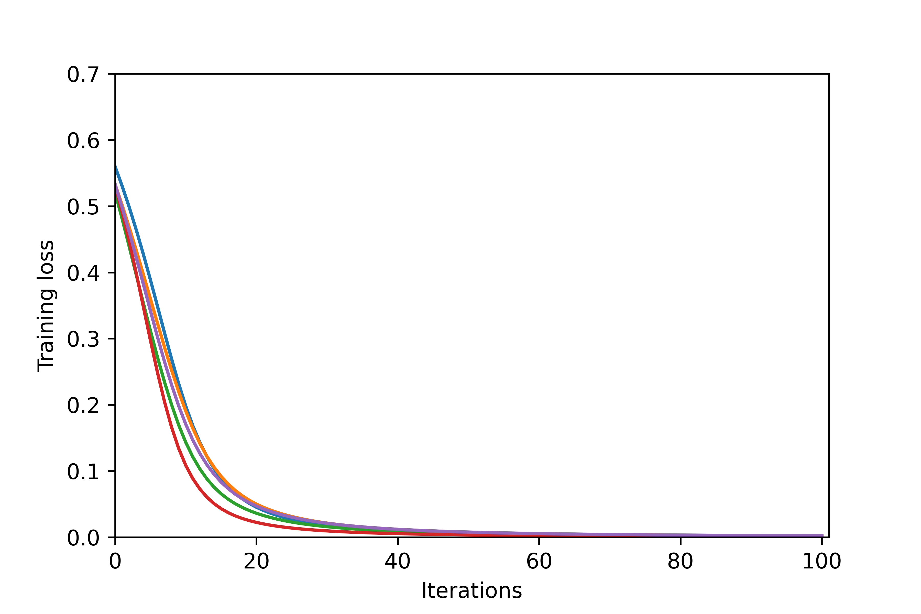
Figure 2: Training loss as a function of the number of gradient descent steps for data distributed as mixtures of Gaussians, where the means have an XOR structure. Details are in Section 5.

We performed a similar collection of simulations, except with a different, more challenging, data distribution, which we call the “shoulders” distribution. The means of the mixture components of the positive examples were $(1,0)$ and $(0,1)$ while the means of mixture components of the negative examples remain at the same place. The positive centers start to crowd the negative center $(1/\sqrt{2},1/\sqrt{2})$ making it more difficult to pick out examples from the negative center. Plots for this data distribution, which also scale roughly like our upper bounds, are shown in Figure 3.

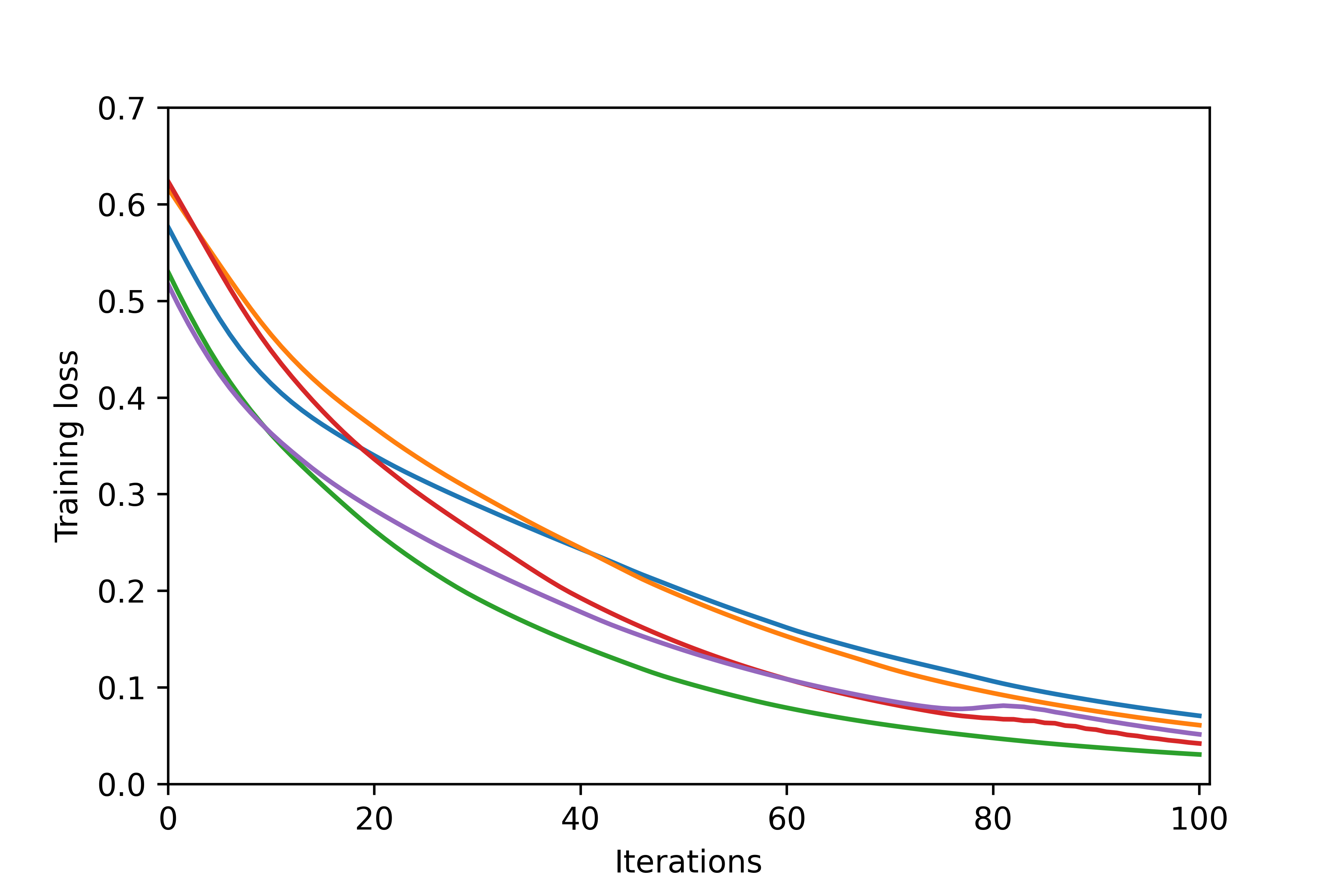
Figure 3: Training loss as a function of the number of gradient descent steps for the “shoulders” distribution. Details are in Section 5.

Next, we performed ten training runs as described above for the shoulders data, except that, for five of them, the Huberized ReLU was replaced by a standard ReLU. The results are in Figure 4. While there is evidence that training with the non-smooth objective arising from the standard ReLU leads to a limited extent of “overshooting”, the shapes of the loss curves agree on a coarser scale.

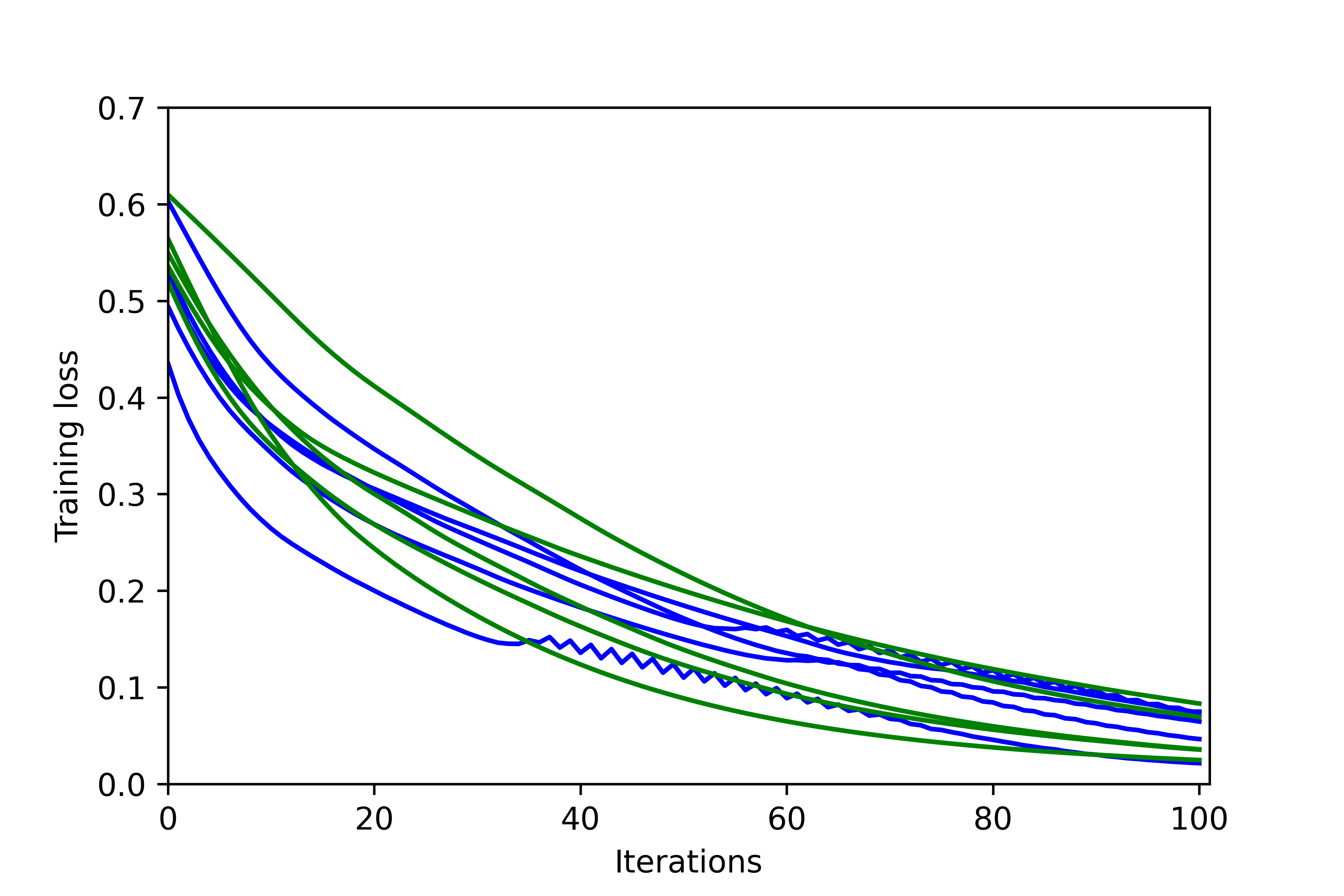
Figure 4: Training loss as a function of the number of gradient descent steps with the ReLU (blue) and the Huberized ReLU (green) on the “shoulders" data.

6 Additional Related Work

[COB19] analyzed gradient flow for a general class of smoothly parameterized models, showing that scaling up the initialization, while scaling down the loss, ensures that a first-order Taylor approximation around the initial solution remains accurate until convergence.

[CB20], building on [CB18, MMM19], show that infinitely wide two-layer squared ReLU networks trained with gradient flow on the logistic loss leads to a max-margin classifier in a particular non-Hilbertian space of functions. (See also the videos in a talk about this work [Chi20].) [Bru+18] show that finite-width two-layer leaky ReLU networks can be trained up to zero-loss using stochastic gradient descent with the hinge loss, when the underlying data is linearly separable.

The papers [BG19, Wei+19, JT19a] identify when it is possible to efficiently learn XOR-type data using neural networks with stochastic gradient descent on the logistic loss.

[Che+20] analyzed regularized training with gradient flow on infinitely wide networks. When training is regularized, the weights also may travel far from their initial values.

Our study is motivated in part by the line of work that has emerged which emphasizes the need to understand the behavior of interpolating (zero training loss/error) classifiers and regressors [Zha+17, Bel+19, see, e.g.,]. A number of recent papers have analyzed the properties of interpolating methods in linear regression [Has+19, Bar+20, Mut+20a, TB20, BL20], linear classification [Mon+19, CL21, LS20, Mut+20, HMX20], kernel regression [LR20, MM19, LRZ20] and simplicial nearest neighbor methods [BHM18].

Also related are the papers that study the implicit bias of gradient methods [NTS15, Sou+18, JT19b, Gun+18, Gun+18a, LMZ18, Aro+19, JT19].

A number of recent papers also theoretically study the optimization of neural networks including [And+14, LY17, Zho+17, Zha+17a, GLM18, PSZ18, Du+18, SS18, Zha+19, Aro+19a, Dan20, DM20, BN20].

In particular, the proof of [DM20] demonstrated that the first iteration of gradient descent learned useful features for the parity-learning problem studied there.

7 Discussion

We demonstrated that gradient descent drives the logistic loss of finite-width two-layer Huberized ReLU networks to zero if the initial loss is small enough. This result makes no assumptions about the width or the number of samples. We also showed that when the data is structured, and the data satisfies certain cluster and separation conditions, random initialization followed by gradient descent drives the loss to zero.

After a preliminary version of this paper was posted on arXiv [CLB20], related results were obtained [CLB21] for deep networks with smoothed approximations to the ReLU, under conditions that include Swish. This analysis included adapting the NTK techniques to these activation functions. This provides a broader set of circumstances under which Theorem 1 of this paper can be applied.

Another interesting way forward would be to examine whether the loss can be shown to decrease super-polynomially with the width when there are more than two clusters per label or if the number of samples per cluster is imbalanced.

It would be interesting to see if the corresponding results hold for ReLU activations, which, despite the success of Swish, remain popular.

Now that we have established conditions under which gradient descent can drive the training error to zero, future work could study the implicit bias of this limit and potentially use this to study the generalization behavior of the final interpolating solution. One step towards this could be establish a more precise directional alignment result to show that gradient descent maximizes the margin of Huberized ReLU networks for logistic loss [LL20, JT20, as].

Theorems 1 and 2 use a concrete choice of a learning rate schedule (at least, up to a constant factor). We believe that our techniques can be extended to apply to a wider variety of learning-rate schedules, with corresponding changes to the convergence rate.

In our paper, we assumed that the features are all unit-length vectors to simplify the proofs. We believe that the results of Theorem 1 can be easily extended to the case where the features have arbitrary bounded lengths. We also expect that the results of Theorem 2 can be extended to the case where the examples in the four clusters are drawn from sub-Gaussian distributions with suitably small variances.

Acknowledgements

We thank Zeshun Zong for alerting us to a mistake in an earlier version of this paper.

We gratefully acknowledge the support of the NSF through grants DMS-2031883 and DMS-2023505 and the Simons Foundation through award 814639.

Appendix A Reduction to the Case of No Bias

Denoting the components of $x_{s}$ by $x_{s1},\ldots,x_{sd}$, define $\tilde{x}_{s}=(x_{s1}/\sqrt{2},\ldots,x_{sd}/\sqrt{2},1/\sqrt{2})$. We consider the process of training a model using $(\tilde{x}_{1},y_{1}),\ldots,(\tilde{x}_{n},y_{n})$.

Consider

$$(\theta^{(1)},\widetilde{V}^{(1)}),(\theta^{(2)},\widetilde{V}^{(2)}),\ldots$$

defined as follows. First, $\theta^{(1)},\theta^{(2)},\ldots$ are generated as described in Section 2. Each row $\tilde{v}_{i}^{(1)}$ of $\widetilde{V}^{(1)}\in\mathbb{R}^{2p\times(d+1)}$ is $\sqrt{2}(v_{i1}^{(1)},\ldots,v_{id}^{(1)},b_{i}^{(1)})$.

Define $\widetilde{L}$ to be, informally, $L$, but without the bias terms, and applied to

$$(\tilde{x}_{1},y_{1}),\ldots,(\tilde{x}_{n},y_{n}).$$

That is

$$\widetilde{L}(\widetilde{V}):=\frac{1}{n}\sum_{s=1}^{n}\log\left(1+\exp\left(-y_{s}\sum_{i=1}^{2p}u_{i}\phi(\tilde{v}_{i}\cdot\tilde{x}_{s})\right)\right).$$

Then, for $\tilde{\alpha}_{1}=2\alpha_{1},\tilde{\alpha}_{2}=2\alpha_{2},\ldots>0$, we define $\widetilde{V}^{(2)},\widetilde{V}^{(3)},\ldots$ to be the iterates of gradient descent applied to $\widetilde{L}$, except replacing $\alpha_{1},\alpha_{2},\ldots$ by $\tilde{\alpha}_{1},\tilde{\alpha}_{2},\ldots$.

We claim that, for all $t$,

• for all $i$, $\tilde{v}_{i}^{(t)}=\sqrt{2}(v_{i1}^{(t)},\ldots,v_{id}^{(t)},b_{i}^{(t)})$

• for all $i$ and all $s$, $\tilde{v}_{i}^{(t)}\cdot\tilde{x}_{s}=v_{i}^{(t)}\cdot x_{s}+b_{i}^{(t)}$, so that $\widetilde{L}(\widetilde{V}^{(t)})=L(\theta^{(t)})$.

The first condition is easily seen to imply the second. Further, the first condition holds at $t=1$ by construction. What remains is to prove that the inductive hypothesis for iteration $t$ implies the first condition at iteration $t+1$. If $f_{V}$ is the function computed by the network with weights $V$ and no biases, we have

$$\tilde{v}_{i}^{(t+1)} =\tilde{v}_{i}^{(t)}+\tilde{\alpha}_{t}\sum_{s=1}^{n}\frac{1}{1+\exp(y_{s}f_{\widetilde{V}}^{(t)}(\tilde{x}_{s}))}\phi^{\prime}(\tilde{v}_{i}^{(t)}\cdot\tilde{x}_{s})y_{s}u_{i}\tilde{x}_{s}$$

$$=\sqrt{2}(v_{i1}^{(t)},\ldots,v_{id}^{(t)},b_{i}^{(t)})+\tilde{\alpha}_{t}\sum_{s=1}^{n}\frac{1}{1+\exp(y_{s}f_{\theta}^{(t)}(x_{s}))}\phi^{\prime}(v_{i}^{(t)}\cdot x_{s}+b_{i}^{(t)})y_{s}u_{i}\tilde{x}_{s}$$

(by the inductive hypothesis)

$$=\sqrt{2}(v_{i1}^{(t+1)},\ldots,v_{id}^{(t+1)},b_{i}^{(t+1)}),$$

because $\tilde{x}_{s}=(x_{s1}/\sqrt{2},\ldots,x_{sd}/\sqrt{2},1/\sqrt{2})$ and $\tilde{\alpha}_{t}=2\alpha_{t}$, completing the induction.

Finally, note that

$$\tilde{x}_{s}\cdot\tilde{x}_{q}=\frac{x_{s}\cdot x_{q}+1}{2}\geq 0,$$

since $x_{s}$ and $x_{q}$ are unit length.

Appendix B Omitted Proofs from Section 3.3

In this section we provide proofs of Lemmas 5-8.

B.1 Proof of Lemma 5

See 5

Proof For any $W\in[V^{(t)},V^{t+1}]$ we have that

$$\nabla_{W}L(W)-\nabla L_{t} =\int_{0}^{1}\left(\nabla^{2}_{\bar{W}}L|_{\bar{W}=sV^{(t)}+(1-s)W}\right)(W-V^{(t)})\;\mathrm{d}s,$$

where, as stated above, the weak Hessian is defined using the weak derivative $\gamma$ of $\phi^{\prime}$. Thus,

$$\lVert\nabla_{W}L(W)-\nabla L_{t}\rVert \leq\left[\sup_{s\in[0,1]}\left\lVert\nabla^{2}_{\bar{W}}L|_{\bar{W}=sV^{(t)}+(1-s)W}\right\rVert_{op}\right]\lVert W-V^{(t)}\rVert\leq M\lVert W-V^{(t)}\rVert.$$

This shows that along the line segment joining $V^{(t)}$ to $V^{(t+1)}$ the function is $M$-smooth. Therefore, by using a standard argument [Bub15, see, e.g,] we get that

$$L_{t+1} \leq L_{t}+\nabla L_{t}\cdot(V^{(t+1)}-V^{(t)})+\frac{M}{2}\lVert V^{(t+1)}-V^{(t)}\rVert^{2}$$

$$=L_{t}-\alpha_{t}\lVert\nabla L_{t}\rVert^{2}+\frac{\alpha_{t}^{2}M}{2}\lVert\nabla L_{t}\rVert^{2}$$

$$=L_{t}-\alpha_{t}\left(1-\frac{\alpha_{t}M}{2}\right)\lVert\nabla L_{t}\rVert^{2}$$

$$\leq L_{t}-\frac{5\alpha_{t}\lVert\nabla L_{t}\rVert^{2}}{6}.$$

This completes the proof.  

B.2 Proof of Lemma 6

See 6

Proof  We know that the gradient of the loss with respect to $v_{i}$ is

$$\nabla_{v_{i}}L=\frac{-u_{i}}{n}\sum_{s=1}^{n}\frac{\phi^{\prime}(v_{i}\cdot x_{s})y_{s}x_{s}}{1+\exp\left(y_{s}f_{V}(x_{s})\right)}.$$

The weak Hessian $\nabla^{2}L$ is a block matrix with $4p^{2}$ blocks, where the $(i,j)^{th}$ block is $\nabla_{v_{i}}\nabla_{v_{j}}L$.

First, if $i\neq j$

$$\nabla_{v_{i}}\nabla_{v_{j}}L=\frac{u_{i}u_{j}}{n}\sum_{s=1}^{n}\frac{\phi^{\prime}(v_{i}\cdot x_{s})\phi^{\prime}(v_{j}\cdot x_{s})\exp(y_{s}f_{V}(x_{s}))}{\left(1+\exp\left(y_{s}f_{V}(x_{s})\right)\right)^{2}}x_{s}x_{s}^{\top}.$$ (21)

If $i=j$,

$$\nabla^{2}_{v_{i}}L=\frac{1}{n}\sum_{s=1}^{n}\left[\frac{-u_{i}\gamma(v_{i}\cdot x_{s})y_{s}}{1+\exp\left(y_{s}f_{V}(x_{s})\right)}+\frac{\phi^{\prime}(v_{i}\cdot x_{s})^{2}\exp(y_{s}f_{V}(x_{s}))}{\left(1+\exp\left(y_{s}f_{V}(x_{s})\right)\right)^{2}}\right]x_{s}x_{s}^{\top}.$$ (22)

By definition of the operator norm,

$$\lVert\nabla^{2}_{V}L\rVert_{op}=\sup_{a:\lVert a\rVert=1}\left\lVert\left(\nabla^{2}_{V}L\right)a\right\rVert.$$ (23)

Let $a$ be a unit length member of $\mathbb{R}^{2p(d+1)}$ and let us decompose $a$ into segments $a_{1},\ldots,a_{2p}$ of $(d+1)$ components each, so that $a$ is the concatenation of $a_{1},\ldots,a_{2p}\in\mathbb{R}^{d+1}$. Note that $\sum_{i=1}^{2p}\lVert a_{i}\rVert^{2}=1$.

The squared norm of $(\nabla^{2}L)a$ is

$$\left\lVert(\nabla^{2}L)a\right\rVert^{2} =\sum_{i\in[2p]}\left\lVert\sum_{j\in[2p]}\left(\nabla_{v_{i}}\nabla_{v_{j}}L\right)a_{j}\right\rVert^{2}$$

$$=\sum_{i,j,k\in[2p]}a_{k}^{\top}\left[\left(\nabla_{v_{i}}\nabla_{v_{k}}L\right)\left(\nabla_{v_{i}}\nabla_{v_{j}}L\right)\right]a_{j}$$

$$\leq\sum_{i,j,k\in[2p]}\lVert a_{j}\rVert\lVert a_{k}\rVert\lVert\nabla_{v_{i}}\nabla_{v_{k}}L\rVert_{op}\lVert\nabla_{v_{i}}\nabla_{v_{j}}L\rVert_{op}.$$ (24)

By definition of the Huberized ReLU (in equation (1)) and its weak Hessian (in equation (4)) we know that, for any $z\in\mathbb{R}$, $\lvert\phi^{\prime}(z)\rvert<1$ and $\lvert\gamma(z)\rvert<1/h$. Further, by Lemma 20, we know that for all $s$

$$\frac{\exp(y_{s}f_{V}(x_{s}))}{\left(1+\exp\left(y_{s}f_{V}(x_{s})\right)\right)^{2}}\leq\frac{1}{1+\exp\left(y_{s}f_{V}(x_{s})\right)}\leq L(V;x_{s},y_{s})=\log(1+\exp(-y_{s}f_{V}(x_{s}))).$$

Also recall that for all $s\in[n]$, $\lVert x_{s}\rVert=1$ and for all $i\in[2p]$, $\lvert u_{i}\rvert=1$. Applying these to equation (21), when $i\neq j$ we get that

$$\lVert\left(\nabla_{v_{i}}\nabla_{v_{j}}L\right)\rVert_{op}\leq L,$$ (25)

and, using equation (22), when $i=j$ yields the bound

$$\lVert\nabla^{2}_{v_{i}}L\rVert_{op}\leq L\left(1+\frac{1}{h}\right)\leq 2L/h.$$ (26)

Returning to inequality (24),

$$\left\lVert(\nabla^{2}L)a\right\rVert^{2} \leq\sum_{i,j,k\in[2p]}\lVert a_{j}\rVert\lVert a_{k}\rVert\lVert\nabla_{v_{i}}\nabla_{v_{k}}L\rVert_{op}\lVert\nabla_{v_{i}}\nabla_{v_{j}}L\rVert_{op}$$

$$=\sum_{i,j,k\in[2p]:i=j=k}\lVert a_{j}\rVert^{2}\lVert\nabla^{2}_{v_{i}}L\rVert_{op}^{2}$$

$$\qquad+\sum_{i,j,k\in[2p]:(i\neq j)\wedge(i\neq k)}\lVert a_{j}\rVert\lVert a_{k}\rVert\lVert\nabla_{v_{i}}\nabla_{v_{k}}L\rVert_{op}\lVert\nabla_{v_{i}}\nabla_{v_{j}}L\rVert_{op}$$

$$\qquad+\sum_{i,j,k\in[2p]:i=j\neq k}\lVert a_{j}\rVert\lVert a_{k}\rVert\lVert\nabla_{v_{i}}\nabla_{v_{k}}L\rVert_{op}\lVert\nabla^{2}_{v_{i}}L\rVert_{op}$$

$$\qquad+\sum_{i,j,k\in[2p]:i=k\neq j}\lVert a_{j}\rVert\lVert a_{k}\rVert\lVert\nabla_{v_{i}}\nabla_{v_{j}}L\rVert_{op}\lVert\nabla^{2}_{v_{i}}L\rVert_{op}.$$ (27)

Recall that $h=1/p$, therefore, by inequality (26), the first term in the inequality above can be bounded by

$$\sum_{i,j,k\in[2p]:i=j=k}\lVert a_{j}\rVert^{2}\lVert\nabla^{2}_{v_{i}}L\rVert_{op}^{2}\leq(2L/h)^{2}\sum_{j}\lVert a_{j}\rVert^{2}=4L^{2}p^{2}.$$

Using inequality (25), the second term in the RHS of inequality (27) is

$$\sum_{i,j,k\in[2p]:(i\neq j)\wedge(i\neq k)}\lVert a_{j}\rVert\lVert a_{k}\rVert\lVert\nabla_{v_{i}}\nabla_{v_{k}}L\rVert_{op}\lVert\nabla_{v_{i}}\nabla_{v_{j}}L\rVert_{op}$$

$$\qquad\qquad\qquad\leq L^{2}\sum_{i,j,k\in[2p]:(i\neq j)\wedge(i\neq k)}\lVert a_{j}\rVert\lVert a_{k}\rVert$$

$$\qquad\qquad\qquad\leq L^{2}\sum_{i,j,k\in[2p]:(i\neq j)\wedge(i\neq k)}\frac{\lVert a_{j}\rVert^{2}+\lVert a_{k}\rVert^{2}}{2}$$

$$\qquad\qquad\qquad=\frac{(2p-1)L^{2}}{2}\sum_{i\in[2p]}\left(\sum_{j\in[2p]:i\neq j}\lVert a_{j}\rVert^{2}+\sum_{k\in[2p]:i\neq k}\lVert a_{k}\rVert^{2}\right)$$

$$\qquad\qquad\qquad=\frac{(2p-1)L^{2}}{2}\sum_{i\in[2p]}2(1-\lVert a_{i}\rVert^{2})$$

$$\qquad\qquad\qquad=(2p-1)^{2}L^{2}\leq 4p^{2}L^{2}.$$

Finally, the last two terms in inequality (27) can each be bounded by

$$\sum_{i,j,k\in[2p]:i=j\neq k}\lVert a_{j}\rVert\lVert a_{k}\rVert\lVert\nabla_{v_{i}}\nabla_{v_{k}}L\rVert_{op}\lVert\nabla^{2}_{v_{i}}L\rVert_{op} \leq(2L/h)\cdot L\sum_{j,k\in[2p]:j\neq k}\lVert a_{j}\rVert\lVert a_{k}\rVert$$

$$=2pL^{2}\sum_{j,k\in[2p]:j\neq k}\lVert a_{j}\rVert\lVert a_{k}\rVert$$

$$\leq 2pL^{2}\sum_{j,k\in[2p]:j\neq k}\frac{\lVert a_{j}\rVert^{2}+\lVert a_{k}\rVert^{2}}{2}$$

$$=pL^{2}\sum_{j\in[2p]}\left(\lVert a_{j}\rVert^{2}+\sum_{k\in[2p]:k\neq j}\lVert a_{k}\rVert^{2}\right)$$

$$=pL^{2}\sum_{i\in[2p]}\left(\lVert a_{j}\rVert^{2}+(1-\lVert a_{j}\rVert^{2})\right)$$

$$=2p^{2}L^{2}.$$

The bounds on these four terms combined with inequality (27) tells us that

$$\left\lVert(\nabla^{2}L)a\right\rVert^{2} \leq 12L^{2}p^{2}.$$

Taking square roots along with the definition of the operator norm in equation (23) completes the proof.  

B.3 Proof of Lemma 7

See 7

Proof  Recall the definition of $g_{s}=\left(1+\exp\left(y_{s}f_{V}(x_{s})\right)\right)^{-1}$. By using the expression for the gradient of the loss

$$\lVert\nabla_{V}L\rVert^{2} =\sum_{i=1}^{2p}\lVert\nabla_{v_{i}}L(V)\rVert^{2}$$

$$=\frac{1}{n^{2}}\sum_{i=1}^{2p}\left\lVert\sum_{s=1}^{n}g_{s}\phi^{\prime}(v_{i}\cdot x_{s})y_{s}x_{s}\right\rVert^{2}$$

$$=\frac{1}{n^{2}}\sum_{i=1}^{2p}\sum_{s=1}^{n}\sum_{q=1}^{n}g_{s}g_{q}\phi^{\prime}(v_{i}\cdot x_{s})\phi^{\prime}(v_{i}\cdot x_{q})y_{s}y_{q}x_{s}\cdot x_{q}.$$

By definition we know that $\lvert\phi^{\prime}(v_{i}\cdot x_{s})\rvert<1$ for all $s\in[n]$ and $\lvert y_{s}y_{q}x_{s}\cdot x_{q}\rvert\leq 1$ for any pair $s,q\in[n]$. Therefore,

$$\lVert\nabla_{V}L\rVert^{2} \leq\frac{1}{n^{2}}\sum_{i=1}^{2p}\sum_{s=1}^{n}\sum_{q=1}^{n}g_{s}g_{q}=\frac{2p}{n^{2}}\sum_{s=1}^{n}\sum_{q=1}^{n}g_{s}g_{q}.$$

Since $g_{k},g_{\ell}\leq 1$, this implies $\lVert\nabla_{V}L\rVert^{2}\leq 2p$.

To get the stronger bound when $L(V)$ is small, by Lemma 20, Part 1 we know that $g_{s}g_{q}\leq L_{s}L_{q}$. Thus,

$$\lVert\nabla_{V}L\rVert^{2} \leq\frac{2p}{n^{2}}\left(\sum_{s=1}^{n}\sum_{q=1}^{n}L_{s}L_{q}\right)=2p\left(\frac{1}{n}\sum_{s=1}^{n}L_{s}\right)^{2}=2pL(V)^{2}$$

completing the proof.  

B.4 Proof of Lemma 8

See 8

Proof  In order to apply Lemma 5, we would like to bound $\lVert\nabla^{2}_{W}L\rVert_{op}$ for all convex combinations $W$ of $V^{(t)}$ and $V^{(t+1)}$. For $N={\left\lceil\frac{\sqrt{2p}\lVert V^{(t+1)}-V^{(t)}\rVert}{L_{t}}\right\rceil}$, we will prove the following by induction:

For all $s\in\{0,\ldots,N\}$, for all $\eta\in[0,s/N]$, for $W=\eta V^{(t+1)}+(1-\eta)V^{(t)}$, $\lVert\nabla^{2}_{W}L\rVert_{op}\leq 10pL_{t}$.

The base case, where $s=0$ follows directly from Lemma 6. Now, assume that the inductive hypothesis holds from some $s$, and, for $\eta\in(s/N,(s+1)/N]$, consider $W=\eta V^{(t+1)}+(1-\eta)V^{(t)}$. Let $\widetilde{W}=(s/N)V^{(t+1)}+(1-s/N)V^{(t)}$. Applying Lemma 5 along with the inductive hypothesis, $L(\widetilde{W})\leq L_{t}$. Applying Lemma 7,

$$L(W) \leq L(\widetilde{W})+(\sqrt{2p})\lVert W-\widetilde{W}\rVert$$

$$\leq L_{t}+\frac{\sqrt{2p}\lVert V^{(t+1)}-V^{(t)}\rVert}{N}$$

$$\leq 2L_{t}.$$

Applying Lemma 6, this implies $\lVert\nabla^{2}_{W}L\rVert_{op}\leq 10pL(V^{(t)})$, completing the proof of the inductive step.

So, now we know that, for all convex combinations $W$ of $V^{(t)}$ and $V^{(t+1)}$, $\lVert\nabla^{2}_{W}L\rVert_{op}\leq 10pL(V^{(t)})$. Applying Lemma 5, we have

$$L_{t+1} \leq L_{t}-\frac{5\alpha_{t}\lVert\nabla L_{t}\rVert^{2}}{6},$$

which is the desired result.  

B.5 Proof of Lemma 9

See 9

Proof  If $n=1$ the lemma is trivial. Consider the case $n>1$. Consider an arbitrary feasible point $z_{1},\ldots,z_{n}$ with $z_{1},\ldots,z_{n}>0$ and $\sum_{i=1}^{n}z_{i}=M$. Assume without loss of generality that $z_{1}\geq z_{2}\geq\ldots\geq z_{n}$. For an arbitrarily small $\eta>0$, we claim that the point $z_{1}+z_{2}-\eta,\eta,z_{3},\ldots,z_{n}$ is at least as good. Since $\psi$ is concave

$$\psi(z_{1}) \geq\frac{z_{2}-\eta}{z_{1}+z_{2}-2\eta}\psi(\eta)+\frac{z_{1}-\eta}{z_{1}+z_{2}-2\eta}\psi(z_{1}+z_{2}-\eta),\quad\mbox{ and }$$

$$\psi(z_{2}) \geq\frac{z_{1}-\eta}{z_{1}+z_{2}-2\eta}\psi(\eta)+\frac{z_{2}-\eta}{z_{1}+z_{2}-2\eta}\psi(z_{1}+z_{2}-\eta).$$

So by adding these two inequalities we infer

$$\psi(z_{1}+z_{2}-\eta)+\psi(\eta)+\sum_{i=3}^{n}\psi(z_{i}) \leq\psi(z_{1})+\psi(z_{2})+\sum_{i=3}^{n}\psi(z_{i}).$$

Repeating this for the other $(n-2)$ components of the solution, we find that

$$\psi(M-(n-1)\eta)+(n-1)\psi(\eta) \leq\sum_{i=1}^{n}\psi(z_{i}).$$

Since $\psi$ is a continuous function by taking the limit $\eta\to 0^{+}$ we get that,

$$\psi(M)+(n-1)\lim_{\eta\to 0^{+}}\psi(\eta) \leq\sum_{i=1}^{n}\psi(z_{i}).$$

Given that $z_{1},\ldots,z_{n}$ was an arbitrary feasible point, the previous inequality establishes our claim.  

Appendix C Reduction to the Case of No Bias with Random Initialization

We once again consider the process of training a model using $(\tilde{x}_{1},y_{1}),\ldots,(\tilde{x}_{n},y_{n})$, where $\tilde{x}_{s}$ is defined as in Appendix A.

Let $\widetilde{\sigma}=\sqrt{2}\sigma$. A sample from $\mathcal{N}(0,\widetilde{\sigma}^{2})$ can be generated by sampling from $\mathcal{N}(0,\sigma^{2})$, and scaling the result up by a factor of $\sqrt{2}$.

For some $\sigma>0$, and $\alpha_{0},\alpha_{1},\alpha_{2},\ldots>0$, $h\geq 0$, consider the joint distribution on

$$(\theta^{(0)},\widetilde{V}^{(0)}),(\theta^{(1)},\widetilde{V}^{(1)}),\ldots$$

defined as follows. First, $\theta^{(0)},\theta^{(1)},\ldots$ are generated as described in Section 2.4. Each row $\tilde{v}_{i}^{(0)}$ of $\widetilde{V}^{(0)}\in\mathbb{R}^{2p\times(d+1)}$ is $\sqrt{2}(v_{i1}^{(0)},\ldots,v_{id}^{(0)},b_{i}^{(0)})$ (so that they are mutually independent draws from ${\cal N}(0,2\sigma^{2})$).

Define $\widetilde{L}$ as in Appendix A: informally, $L$, but without the bias terms.

Then, for $\tilde{\alpha}_{0}=2\alpha_{0},\tilde{\alpha}_{1}=2\alpha_{1},\ldots>0$, we define $\widetilde{V}^{(1)},\widetilde{V}^{(2)},\ldots$ to be the iterates of gradient descent applied to $\widetilde{L}$, except replacing $\alpha_{0},\alpha_{1},\alpha_{2},\ldots$ by $\tilde{\alpha}_{0},\tilde{\alpha}_{1},\tilde{\alpha}_{2},\ldots$.

Arguing as in Appendix A, except starting with round $0$, we can see that, for all $t$,

• for all $i$, $\tilde{v}_{i}^{(t)}=\sqrt{2}(v_{i1}^{(t)},\ldots,v_{id}^{(t)},b_{i}^{(t)})$

• for all $i$ and all $s$, $\tilde{v}_{i}^{(t)}\cdot\tilde{x}_{s}=v_{i}^{(t)}\cdot x_{s}+b_{i}^{(t)}$, so that $\widetilde{L}(\widetilde{V}^{(t)})=L(\theta^{(t)})$.

For each cluster $k$, define $\tilde{\mu}_{k}$ by $\tilde{\mu}_{k}=\left(\frac{\mu_{k1}}{\sqrt{2}},\ldots,\frac{\mu_{kd}}{\sqrt{2}},\frac{1}{\sqrt{2}}\right).$ Note that $\lVert\tilde{x}_{s}-\tilde{\mu}_{k}\rVert=\frac{\lVert x_{s}-\mu_{k}\rVert}{\sqrt{2}}$ and, for all clusters $k$ and $\ell$

$$\tilde{\mu}_{k}\cdot\tilde{\mu}_{\ell}=\frac{\mu_{k}\cdot\mu_{\ell}+1}{2}.$$

Appendix D Proof of Lemma 15

We begin by restating the lemma here. See 15 The different parts of the lemma are proved one at a time in the subsections below. The lemma holds by taking a union bound over all the different parts. Throughout the proof of this lemma we fix the samples $(x_{1},y_{1}),\ldots,(x_{n},y_{n})\in\mathbb{S}^{d-1}\times\{-1,1\}$. Conditioned on their value, for all $i\in[2p]$ and for all $s\in[n]$, the random variables $v_{i}^{(0)}\cdot x_{s}\sim\mathcal{N}(0,\sigma^{2})$.

D.1 Proof of Part 1

Consider a fixed sample $s$. Without loss of generality, suppose that $y_{s}=1$. We want to demonstrate a high probability lower bound on

$$\sum_{i\in I_{+s}}v_{i}^{(0)}\cdot x_{s}=\sum_{i\in[p]}(v_{i}^{(0)}\cdot x_{s})\mathbf{1}_{i\in I_{+s}}.$$

Now the expected value of this sum,

$$\mathbb{E}\left[\sum_{i\in[p]}(v_{i}^{(0)}\cdot x_{s})\mathbf{1}_{i\in I_{+s}}\right] =p\mathbb{E}\left[\left(v_{1}^{(0)}\cdot x_{s}\right)\mathbf{1}_{1\in I_{+s}}\right].$$

Choose the function $\chi$ in the statement of the result to be

$$\chi(h,\alpha_{0},\sigma):=\mathbb{E}\left[\left(v_{1}^{(0)}\cdot x_{s}\right)\mathbf{1}_{1\in I_{+s}}\right].$$

By applying Hoeffding’s inequality [Ver18, see] (since $v_{i}^{(0)}\cdot x_{s}\sim\mathcal{N}(0,\sigma^{2})$, the truncated random variable $(v_{i}^{(0)}\cdot x_{s})\mathbf{1}_{i\in I_{+s}}$ is also $c_{1}\sigma$-sub-Gaussian for an appropriate positive constant $c_{1}$),

$$\mathbb{P}\left[\sum_{i\in I_{+s}}v_{i}^{(0)}\cdot x_{s}\leq\mathbb{E}\left[\sum_{i\in I_{+s}}(v_{i}^{(0)}\cdot x_{s})\right]-\eta p\right] \leq\exp\left(-c_{2}\eta^{2}p/\sigma^{2}\right)$$

$$=\exp\left(-c_{2}\eta^{2}p^{2+\beta}\right)$$

since $\sigma=1/p^{1/2+\beta/2}$. Setting $\eta=1/p$ we get

$$\mathbb{P}\left[\sum_{i\in I_{+s}}v_{i}^{(0)}\cdot x_{s}\leq\mathbb{E}\left[\sum_{i\in I_{+s}}(v_{i}^{(0)}\cdot x_{s})\right]-1\right]\leq\exp\left(-c_{2}p^{\beta}\right).$$

Since $p\geq\log^{C_{3}}(nd/\delta)$, for any $C_{3}\geq c_{3}/\beta$, for a large enough constant $c_{3}$ we can establish that

$$\mathbb{P}\left[\sum_{i\in I_{+s}}v_{i}^{(0)}\cdot x_{s}\leq\mathbb{E}\left[\sum_{i\in I_{+s}}(v_{i}^{(0)}\cdot x_{s})\right]-1\right]\leq\frac{\delta}{20n}.$$

Finally, a union bound over all $n$ samples completes the proof for $I_{+s}$:

$$\mathbb{P}\left[\exists s\in[n]:\sum_{i\in I_{+s}}v_{i}^{(0)}\cdot x_{s}\leq\mathbb{E}\left[\sum_{i\in I_{+s}}(v_{i}^{(0)}\cdot x_{s})\right]-1\right]\leq\frac{\delta}{20}.$$

An identical argument holds for the sum: $\sum_{i\in{I_{-s}}}v_{i}^{(0)}\cdot x_{s}$ which completes the proof of this part of the lemma.

D.2 Proof of Part 2

Consider a sample $s$. Without loss of generality, suppose that $y_{s}=1$. Recall the definition of the set

$$I_{+s}=\{i\in[2p]:v_{i}^{(0)}\cdot x_{s}\geq h+4\alpha_{0}\text{ and }u_{i}=y_{s}=1\}.$$

Note that the variable $v_{i}^{(0)}\cdot x_{s}$ has a Gaussian distribution with zero-mean and variance $\sigma^{2}$. Also, recall that $u_{i}=1$ for all $i\in[p]$. Therefore, for each $i\in[p]$,

$$\zeta:=\mathbb{P}\left[v_{i}^{(0)}\cdot x_{s}\geq h+4\alpha_{0}\right] =\frac{1}{2}-\mathbb{P}\left[v_{i}^{(0)}\cdot x_{s}\in[0,h+4\alpha_{0}]\right]$$

$$\overset{(i)}{=}\frac{1}{2}-O\left(\frac{h+\alpha_{0}}{\sigma}\right)$$

$$=\frac{1}{2}-O\left(\frac{1/p+1/p^{1/2+\beta}}{1/p^{1/2+\beta/2}}\right)$$

$$=\frac{1}{2}-o(1),$$

where $(i)$ follows by an upper bound of $1/(\sigma\sqrt{2\pi})$ on the density of a Gaussian random variable with variance $\sigma^{2}$. A Hoeffding bound implies that, for any $\eta>0$

$$\mathbb{P}\left[\Big{\lvert}\left\lvert I_{+s}\right\rvert-\zeta p\Big{\rvert}\geq\eta p\right]\leq 2\exp\left(-c^{\prime}\eta^{2}p\right).$$

Thus by a union bound over all samples

$$\mathbb{P}\left[\exists s\in[n]:\Big{|}\lvert I_{+s}\rvert-\zeta p\Big{|}\geq\eta p\right]\leq 2n\exp\left(-c^{\prime}\eta^{2}p\right).$$

Setting $\eta=1/p^{1/4}$ and recalling that $\zeta=1/2-o(1)$ and $p\geq\log^{C_{3}}(nd/\delta)$ completes the argument for the sets $I_{+s}$. An identical argument goes through for the second claim that establishes a bound on the size of the sets $I_{-s}$.

D.3 Proof of Part 3

By definition $g_{0s}=\left(1+\exp\left(y_{s}\sum_{i=1}^{2p}u_{i}\phi(v_{i}^{0}\cdot x_{s})\right)\right)^{-1}$. Recall that $v_{i}^{(0)}$ is drawn from a zero-mean Gaussian with variance $\sigma^{2}I$. Therefore, for each $i$, $v_{i}^{(0)}\cdot x_{s}$ is a zero-mean Gaussian with variance $\sigma^{2}$ (since $\lVert x_{s}\rVert=1$). For ease of notation let us define $\xi_{i}:=v_{i}^{(0)}\cdot x_{s}$. The sigmoid function $1/(1+\exp(t))$ is $1$-Lipschitz. Therefore,

$$\left\lvert\frac{1}{1+\exp\left(y_{s}\sum_{i=1}^{2p}u_{i}\phi(\xi_{i})\right)}-\frac{1}{1+\exp\left(y_{s}\mathbb{E}\left[\sum_{i=1}^{2p}u_{i}\phi(\xi_{i})\right]\right)}\right\rvert$$

$$\qquad\qquad\qquad\qquad\qquad\qquad\qquad\qquad\qquad\qquad\qquad\qquad\leq\left\lvert\sum_{i=1}^{2p}u_{i}\phi(\xi_{i})-\mathbb{E}\left[\sum_{i=1}^{2p}u_{i}\phi(\xi_{i})\right]\right\rvert.$$

Additionally, by its definition the Huberized ReLU $\phi$ is also $1$-Lipschitz. Therefore for any pair $z_{1},z_{2}\in\mathbb{R}^{2p}$

$$\left\lvert\sum_{i=1}^{2p}u_{i}\left(\phi(z_{1i})-\phi(z_{2i})\right)\right\rvert\leq\sum_{i=1}^{2p}\left\lvert\phi(z_{1i})-\phi(z_{2i})\right\rvert\leq\sum_{i=1}^{2p}\left\lvert z_{1i}-z_{2i}\right\rvert =\lVert z_{1}-z_{2}\rVert_{1}$$

$$\leq\sqrt{2p}\lVert z_{1}-z_{2}\rVert.$$

Hence, the function $y_{s}\sum_{i=1}^{2p}u_{i}\phi(\xi_{i})$ is $\sqrt{2p}$-Lipschitz with respect to its argument

$$(\xi_{1},\ldots,\xi_{2p}).$$

By the Borell-Tsirelson-Ibragimov-Sudakov inequality for the concentration of Lipschitz functions of Gaussian random variables [Wai19, see],

$$\mathbb{P}\left[\left\lvert\sum_{i=1}^{2p}u_{i}\phi(\xi_{i})-\mathbb{E}\left[\sum_{i=1}^{2p}u_{i}\phi(\xi_{i})\right]\right\rvert\geq\eta\right]\leq 2\exp\left(-\frac{\eta^{2}}{4p\sigma^{2}}\right).$$

Recall that $\sigma=1/p^{1/2+\beta/2}$, thus,

$$\mathbb{P}\left[\left\lvert\sum_{i=1}^{2p}u_{i}\phi(\xi_{i}))-\mathbb{E}\left[\sum_{i=1}^{2p}u_{i}\phi(\xi_{i}))\right]\right\rvert\geq\eta\right]\leq 2\exp\left(-c_{1}p^{\beta}\eta^{2}\right).$$

By choosing $\eta=1/p^{\beta/4}$,

$$\mathbb{P}\left[\left\lvert\sum_{i=1}^{2p}u_{i}\phi(\xi_{i}))-\mathbb{E}\left[\sum_{i=1}^{2p}u_{i}\phi(\xi_{i}))\right]\right\rvert\geq\frac{1}{p^{\beta/4}}\right]\leq 2\exp\left(-c_{2}p^{\beta/2}\right).$$

This tells us that with probability at least $1-2\exp(-c_{2}p^{\beta/2})$,

$$\frac{1}{1+\exp\left(y_{s}\mathbb{E}\left[\sum_{i=1}^{2p}u_{i}\phi(\xi_{i}))\right]\right)}-\frac{1}{p^{\beta/4}} \leq\frac{1}{1+\exp\left(y_{s}\sum_{i=1}^{2p}u_{i}\phi(\xi_{i}))\right)}$$

$$\leq\frac{1}{1+\exp\left(y_{s}\mathbb{E}\left[\sum_{i=1}^{2p}u_{i}\phi(\xi_{i}))\right]\right)}+\frac{1}{p^{\beta/4}}.$$ (28)

Next, we calculate the value of $\mathbb{E}\left[\sum_{i=1}^{2p}u_{i}\phi(\xi_{i}))\right]$. Note that all the random variables $\{\xi_{i}\}_{i\in[2p]}$ are identically distributed. Recall that, $u_{i}=1$ if $i\in\{1,\ldots,p\}$ and $u_{i}=-1$ if $i\in\{p+1,\ldots,2p\}$, thus

$$\mathbb{E}\left[\sum_{i=1}^{2p}u_{i}\phi(\xi_{i})\right] =\mathbb{E}\left[\sum_{i=1}^{p}\phi(\xi_{i})\right]-\mathbb{E}\left[\sum_{i=p+1}^{2p}\phi(\xi_{i})\right]=p\mathbb{E}\left[\phi(\xi_{1})]-p\mathbb{E}[\phi(\xi_{1})\right]=0.$$

Thus by inequality (28) we know that with probability at least $1-2\exp(-c_{2}p^{\beta/2})$

$$\frac{1}{2}-o(1)\leq\frac{1}{1+\exp(y_{s}\sum_{i=1}^{2p}u_{i}\phi(v_{i}^{(0)}\cdot x_{s}))}\leq\frac{1}{2}+o(1).$$

A union bound over all $n$ samples completes the proof, since $p\geq\log^{C_{3}}(nd/\delta)$ for a large enough constant $C_{3}$.

D.4 Proof of Part 4

We will first prove the first claim of this part of the lemma. Without loss of generality consider the cluster ${\cal K}_{1}$ (recall that for all examples $s\in{\cal K}_{1}$, $y_{s}=1$). For any pair $s,q\in{\cal K}_{1}$

$$\mathbb{P}\left[v_{i}^{(0)}\cdot x_{s}\geq h+4\alpha_{0}\text{ and }v_{i}^{(0)}\cdot x_{q}\geq h+4\alpha_{0}\right]$$

$$\geq\mathbb{P}\left[v_{i}^{(0)}\cdot x_{s}\geq 0\text{ and }v_{i}^{(0)}\cdot x_{q}\geq 0\right]-\mathbb{P}[v_{i}^{(0)}\cdot x_{s}\in[0,h+4\alpha_{0}]]-\mathbb{P}[v_{i}^{(0)}\cdot x_{q}\in[0,h+4\alpha_{0}]]$$

$$\overset{(i)}{\geq}\mathbb{P}\left[v_{i}^{(0)}\cdot x_{s}\geq 0\text{ and }v_{i}^{(0)}\cdot x_{q}\geq 0\right]-O\left(\frac{h+\alpha_{0}}{\sigma}\right)$$

$$=\mathbb{P}\left[v_{i}^{(0)}\cdot x_{s}\geq 0\text{ and }v_{i}^{(0)}\cdot x_{q}\geq 0\right]-O\left(\frac{1/p+1/p^{1/2+\beta}}{1/p^{1/2+\beta/2}}\right)$$

$$\overset{(ii)}{=}\frac{1-\arccos(x_{s}\cdot x_{q})/\pi}{2}-o(1)$$

$$\overset{(iii)}{\geq}\frac{1-\arccos(1-2r)/\pi}{2}-o(1)$$

$$\geq\frac{1-\sqrt{r}}{2}-o(1)$$

where $(i)$ follows by an upper bound of $1/(\sqrt{2\pi}\sigma)$ on the density of a Gaussian random variable, $(ii)$ follows by noting that the conditional probability of $v_{i}^{(0)}\cdot x_{q}\geq 0$ conditioned on the event that $v_{i}^{(0)}\cdot x_{s}\geq 0$ is $1-\frac{\arccos(x_{s}\cdot x_{q})}{\pi}$, and $(iii)$ follows since $x_{s}\cdot x_{q}\geq 1-2r$ by Lemma 21.

Define $\zeta:=\mathbb{P}\left[v_{i}^{(0)}\cdot x_{s}\geq h+4\alpha_{0}\text{ and }v_{i}^{(0)}\cdot x_{q}\geq h+4\alpha_{0}\right]$. A Hoeffding bound implies that, for any $\eta>0$

$$\mathbb{P}\left[\left\lvert\left\{i\in[p]:\left(v_{i}^{(0)}\cdot x_{s}\geq h+4\alpha_{0}\right)\wedge\left(v_{i}^{(0)}\cdot x_{q}\geq h+4\alpha_{0}\right)\right\}\right\rvert\leq(\zeta-\eta)p\right]\leq\exp\left(-c_{1}\eta^{2}p\right).$$

Recall the definition of the set $I_{+s}=\left\{i\in[2p]:(u_{i}=y_{s}=1)\wedge\left(v_{i}^{(0)}\cdot x_{s}\geq h+4\alpha_{0}\right)\right\}$. Therefore, a union bound over all sample pairs $s,q\in\mathcal{K}_{1}$ implies that

$$\mathbb{P}\left[\left\lvert\left\{i\in[p]:\forall\;s\in{\cal K}_{1},i\in I_{+s}\right\}\right\rvert\leq(\zeta-\eta)p\right] \leq n^{2}\exp\left(-c_{1}\eta^{2}p\right).$$

Finally, by taking a union bound over all 4 clusters we get that

$$\mathbb{P}\left[\exists k\in[4]:\left\lvert\left\{i\in[2p]:\forall\;s\in{\cal K}_{k},i\in I_{+s}\right\}\right\rvert\leq(\zeta-\eta)p\right] \leq 4n^{2}\exp\left(-c_{1}\eta^{2}p\right).$$

Choosing $\eta=1/p^{1/4}$, recalling that $\zeta\geq(1-\sqrt{r}-o(1))/2$ and $p\geq\log^{C_{3}}(nd/\delta)$ for a large enough constant $C_{3}$ completes the proof of the first claim.

The second claim of this part of the lemma follows by an identical argument.

D.5 Proof of Part 5

Without loss of generality, consider a node $i\in[p]$ with $u_{i}=1$ and a fixed pair $s,q\in[n]$ such that $y_{s}=1$ and $y_{q}=-1$. Since each of $v_{i}^{(0)}\cdot x_{s}$ and $v_{i}^{(0)}\cdot x_{q}$ are distributed as $\mathcal{N}(0,\sigma^{2})$, we have

$$\mathbb{P}[v_{i}^{(0)}\cdot x_{s}\geq h+4\alpha_{0}\mbox{ and }v_{i}^{(0)}\cdot x_{q}\geq 0] \leq\mathbb{P}[v_{i}^{(0)}\cdot x_{s}\geq 0\mbox{ and }v_{i}^{(0)}\cdot x_{q}\geq 0]$$

$$\overset{(i)}{=}\frac{1-\frac{\arccos(x_{s}\cdot x_{q})}{\pi}}{2}$$

$$\overset{(ii)}{\leq}\frac{1-\frac{\arccos((1+\Delta)/2+2r)}{\pi}}{2}$$

$$\leq\frac{1}{3}+\frac{\Delta}{4}+r,$$

if the bound $C_{2}$ on $r$ and $\Delta$ is small enough, where $(i)$ follows by noting that the conditional probability of $v_{i}^{(0)}\cdot x_{q}\geq 0$ conditioned on the event that $v_{i}^{(0)}\cdot x_{s}\geq 0$ is $1-\frac{\arccos(x_{s}\cdot x_{q})}{\pi}$, while $(ii)$ follows since by Lemma 21, $x_{s}\cdot x_{q}\leq(1+\Delta)/2+2r$ for samples where $y_{s}\neq y_{q}$.

Now, define $\zeta:=\mathbb{P}[v_{i}^{0}\cdot x_{s}\geq h+4\alpha_{0}\mbox{ and }v_{i}^{(0)}\cdot x_{q}\geq 0]$; a Hoeffding bound implies that, for any $\eta>0$

$$\mathbb{P}[|\{i\in[p]:v_{i}^{(0)}\cdot x_{s}\geq h+4\alpha_{0}\mbox{ and }v_{i}^{(0)}\cdot x_{q}\geq 0]\}|\geq(\zeta+\eta)p]\leq\exp(-c^{\prime}\eta^{2}p).$$

Choosing $\eta=1/p^{1/4}$ and recalling that $\zeta\leq\frac{1}{3}+\frac{\Delta}{4}+r$ along with a union bound over the pairs of samples completes the proof of the first claim. An identical argument works to establish the second claim.

D.6 Proof of Part 6

Without loss of generality, consider a node $i\in[p+1,\ldots,2p]$ with $u_{i}=-1$ and fix a sample $s$ with $y_{s}=1$. Since each $v_{i}^{0}\cdot x_{s}$ is distributed as $\mathcal{N}(0,\sigma^{2})$, we have,

$$\zeta:=\mathbb{P}\left[-\alpha_{0}(1/2+2(\Delta+r))\leq v_{i}^{(0)}\cdot x_{s}\leq h+4\alpha_{0}\right]\leq\frac{1}{\sigma\sqrt{2\pi}}\left(h+5\alpha_{0}(1+\Delta+r)\right),$$ (29)

where the bound on the probability above follows by an upper bound of $1/(\sqrt{2\pi}\sigma)$ on the density of a Gaussian random variable. A Hoeffding bound implies that, for any $\eta>0$

$$\mathbb{P}\left[\lvert\{i\in\{p+1,\ldots,2p\}:-\alpha_{0}(1/2+2(\Delta+r))\leq v_{i}^{(0)}\cdot x_{s}\leq h+4\alpha_{0}\}\rvert\geq(\zeta+\eta)p\right]$$

$$\leq\exp\left(-c^{\prime}\eta^{2}p\right).$$

By choosing $\eta=\frac{5\alpha_{0}}{\sigma\sqrt{2\pi}}=\frac{5}{\sqrt{2\pi}p^{\beta/2}}$, recalling the upper bound on $\zeta$ established in (29) and a union bound over all the $n$ samples completes the proof since $p\geq\log^{C_{3}}(nd/\delta)$ for a large enough constant $C_{3}$.

D.7 Proof of Part 7

We know that each $v_{i}^{(0)}\sim\mathcal{N}(0,\sigma^{2}I_{(d+1)\times(d+1)})$. Thus by a concentration inequality for the lower tail of a $\chi^{2}$-random variable with $2(d+1)p$ degrees of freedom [LM00, see] we have that, for any $\eta>0$

$$\mathbb{P}\left[\frac{\lVert V^{(0)}\rVert}{\sqrt{2(d+1)p}}\leq\sigma\sqrt{1-\eta}\right]\leq\exp(-(d+1)p\eta^{2}/2).$$

Recall that $\sigma=1/p^{1/2+\beta/2}$, thus by setting $\eta=1/32$ we get that

$$\mathbb{P}\left[\lVert V^{(0)}\rVert\leq\frac{6\sqrt{d+1}}{5p^{\beta/2}}\right]\leq\exp(-c_{1}(d+1)p).$$

Since $p\geq\log^{C_{3}}(nd/\delta)$ for a large enough value of $C_{3}$, this ensures that

$$\lVert V^{(0)}\rVert\geq 6\sqrt{d+1}/(5p^{\beta/2})$$

with probability at least $1-\delta/c_{2}$. By the reverse triangle inequality,

$$\lVert V^{(1)}\rVert \geq\lVert V^{(0)}\rVert-\alpha_{0}\lVert\nabla L_{0}\rVert\overset{(i)}{\geq}\lVert V^{(0)}\rVert-\alpha_{0}\sqrt{2p}\geq\frac{6\sqrt{d+1}}{5p^{\beta/2}}-\frac{\sqrt{2}}{p^{\beta}}\overset{(ii)}{\geq}\frac{3}{5}\sqrt{\frac{d}{p^{\beta}}},$$

where $(i)$ follows by the bound on the norm of gradient established in Lemma 7 and $(ii)$ follows since $d\geq 2$ under our clustering assumptions. Hence

$$\mathbb{P}\left[\lVert V^{(1)}\rVert\geq\frac{3}{5}\sqrt{\frac{d}{p^{\beta}}}\right]\geq 1-\delta/c_{2},$$ (30)

which establishes the desired lower bound on the norm of $V^{(1)}$. To establish the upper bound we will use the Borell-TIS inequality for Lipschitz functions of Gaussian random variables [Wai19, see]. By this inequality we have that, for any $\eta>0$

$$\mathbb{P}\left[\frac{\lVert V^{(0)}\rVert}{\sqrt{2(d+1)p}}\geq\sigma(1+\eta)\right]\leq\exp(-(d+1)p\eta^{2}).$$

Once again because $\sigma=1/p^{1/2+\beta/2}$, by setting $\eta=1/32$ we get that

$$\mathbb{P}\left[\lVert V^{(0)}\rVert\geq\frac{3\sqrt{d+1}}{2p^{\beta/2}}\right]\leq\exp(-c_{1}(d+1)p).$$

Since $p\geq\log^{C_{3}}(nd/\delta)$ for a large enough value of $C_{3}$, this ensures that

$$\lVert V^{(0)}\rVert\leq 3\sqrt{d+1}/(2p^{\beta/2})\leq 5\sqrt{d}/2p^{\beta/2}$$

with probability at least $1-\delta/c_{2}$. By the triangle inequality,

$$\lVert V^{(1)}\rVert \leq\lVert V^{(0)}\rVert+\alpha_{0}\lVert\nabla L_{0}\rVert\overset{(i)}{\leq}\lVert V^{(0)}\rVert+\alpha_{0}\sqrt{2p}\leq\frac{5\sqrt{d}}{2p^{\beta/2}}+\frac{\sqrt{2}}{p^{\beta}}\leq 3\sqrt{\frac{d}{p^{\beta}}},$$

where $(i)$ follows by the bound on the norm of gradient established in Lemma 7. Hence

$$\mathbb{P}\left[\lVert V^{(1)}\rVert\leq 3\sqrt{\frac{d}{p^{\beta}}}\right]\geq 1-\delta/c_{2}.$$

Combining this with inequality (30) above we get that

$$\mathbb{P}\left[\frac{3}{5}\sqrt{\frac{d}{p^{\beta}}}\leq\lVert V^{(1)}\rVert\leq 3\sqrt{\frac{d}{p^{\beta}}}\right]\geq 1-2\delta/c_{2}$$

completing our proof.

Appendix E Auxiliary Lemmas

In this section we list a couple of lemmas that are useful in various proofs above.

Lemma 20.

For any $x\in\mathbb{R}^{d}$ and $y\in\{-1,1\}$ and any weight matrix $V$ we have the following

1. $$\frac{1}{1+\exp\left(yf_{V}(x)\right)}\leq\log(1+\exp(-yf_{V}(x)))=L(V;x,y).$$

2. $$\frac{\exp\left(yf_{V}(x)\right)}{\left(1+\exp\left(yf_{V}(x)\right)\right)^{2}}\leq\frac{1}{1+\exp\left(yf_{V}(x)\right)}\leq L(V;x,y).$$

Proof  Part $1$ follows since for any $z\in\mathbb{R}$, we have the inequality $(1+\exp(z))^{-1}\leq\log(1+\exp(-z))$.

Part $2$ follows since for any $z\in\mathbb{R}^{d}$, we have the inequality $\exp(z)/\left(1+\exp(z)\right)^{2}\leq\left(1+\exp(z)\right)^{-1}$.  

Lemma 21.

Given an $r<1$ suppose that for any $k\in[4]$ all samples $s\in{\cal K}_{k}$ satisfy the bound $\lVert x_{s}-\mu_{k}\rVert\leq r/\sqrt{2}$ and for all $k\in[4]$, $\lVert\mu_{k}\rVert=1$.

1. Then for any pair of clusters ${\cal K}_{k},{\cal K}_{\ell}$ such that $y_{k}\neq y_{\ell}$, and $\mu_{k}\cdot\mu_{\ell}\leq(1+\Delta)/2$ we have, for all $s\in{\cal K}_{k}$ and $q\in{\cal K}_{\ell}$

   $$x_{s}\cdot x_{q}\leq\frac{1+\Delta}{2}+2r.$$

2. Given a cluster ${\cal K}_{k}$, if $s,s^{\prime}\in{\cal K}_{k}$ then,

   $$x_{s}\cdot x_{s^{\prime}}\geq 1-2r.$$

Proof Proof of Part 1: By evaluating the inner product and applying the Cauchy-Schwarz inequality

$$x_{s}\cdot x_{q} =(x_{s}-\mu_{k}+\mu_{k})\cdot(x_{q}-\mu_{\ell}+\mu_{\ell})$$

$$=\mu_{k}\cdot\mu_{\ell}+(x_{s}-\mu_{k})\cdot\mu_{\ell}+\mu_{k}\cdot(x_{q}-\mu_{\ell})+(x_{s}-\mu_{k})\cdot(x_{q}-\mu_{\ell})$$

$$\leq\frac{1+\Delta}{2}+\sqrt{2}r+\frac{r^{2}}{2}$$

$$\leq\frac{1+\Delta}{2}+2r.$$

Proof of Part 2: Recall that $\lVert\mu_{k}\rVert=1$. Thus, given two samples $s,s^{\prime}\in{\cal K}_{k}$,

$$x_{s}\cdot x_{s}^{\prime} =(x_{s}-\mu_{k}+\mu_{k})\cdot(x_{s^{\prime}}-\mu_{k}+\mu_{k})$$

$$=\mu_{k}\cdot\mu_{k}+(x_{s}-\mu_{k})\cdot\mu_{k}+\mu_{k}\cdot(x_{s^{\prime}}-\mu_{k})+(x_{s}-\mu_{k})\cdot(x_{s^{\prime}}-\mu_{k})$$

$$\geq 1-\sqrt{2}r-\frac{r^{2}}{2}$$

$$\geq 1-2r$$

as claimed.

References

- [ALS19] Zeyuan Allen-Zhu, Yuanzhi Li and Zhao Song “A convergence theory for deep learning via over-parameterization” In International Conference on Machine Learning, 2019, pp. 242–252
- [And+14] Alexandr Andoni, Rina Panigrahy, Gregory Valiant and Li Zhang “Learning polynomials with neural networks” In International Conference on Machine Learning, 2014, pp. 1908–1916
- [Aro+19] Sanjeev Arora, Nadav Cohen, Wei Hu and Yuping Luo “Implicit regularization in deep matrix factorization” In Advances in Neural Information Processing Systems, 2019, pp. 7413–7424
- [Aro+19a] Sanjeev Arora, Simon S Du, Wei Hu, Zhiyuan Li and Ruosong Wang “Fine-grained analysis of optimization and generalization for overparameterized two-layer neural networks” In International Conference on Machine Learning, 2019, pp. 322–332
- [BL20] Peter L Bartlett and Philip M Long “Failures of model-dependent generalization bounds for least-norm interpolation” In arXiv preprint arXiv:2010.08479, 2020
- [Bar+20] Peter L Bartlett, Philip M Long, Gábor Lugosi and Alexander Tsigler “Benign overfitting in linear regression” In Proceedings of the National Academy of Sciences 117.48, 2020, pp. 30063–30070
- [Bel+19] Mikhail Belkin, Daniel J Hsu, Siyuan Ma and Soumik Mandal “Reconciling modern machine-learning practice and the classical bias–variance trade-off” In Proceedings of the National Academy of Sciences 116.32, 2019, pp. 15849–15854
- [BHM18] Mikhail Belkin, Daniel J Hsu and Partha Mitra “Overfitting or perfect fitting? Risk bounds for classification and regression rules that interpolate” In Advances in Neural Information Processing Systems, 2018, pp. 2300–2311
- [BN20] Guy Bresler and Dheeraj Nagaraj “A corrective view of neural networks: Representation, memorization and learning” In Conference on Learning Theory, 2020, pp. 848–901
- [BG19] Alon Brutzkus and Amir Globerson “Why do larger models generalize better? A theoretical perspective via the XOR problem” In International Conference on Machine Learning, 2019, pp. 822–830
- [Bru+18] Alon Brutzkus, Amir Globerson, Eran Malach and Shai Shalev-Shwartz “SGD learns over-parameterized networks that provably generalize on linearly separable data” In International Conference on Learning Representations, 2018
- [Bub15] Sébastien Bubeck “Convex optimization: algorithms and complexity” In Foundations and Trends® in Machine Learning 8.3-4 Now Publishers, Inc., 2015, pp. 231–357
- [CL21] Niladri S Chatterji and Philip M Long “Finite-sample analysis of interpolating linear classifiers in the overparameterized regime” In Journal of Machine Learning Research 22.129, 2021, pp. 1–30
- [CLB20] Niladri S Chatterji, Philip M Long and Peter L Bartlett “When does gradient descent with logistic loss find interpolating two-layer networks?” In arXiv preprint arXiv:2012.02409, 2020
- [CLB21] Niladri S Chatterji, Philip M Long and Peter L Bartlett “When does gradient descent with logistic loss interpolate using deep networks with smoothed ReLU activations?” In Conference on Learning Theory, 2021
- [Che+20] Zixiang Chen, Yuan Cao, Quanquan Gu and Tong Zhang “A generalized neural tangent kernel analysis for two-layer neural networks” In Advances in Neural Information Processing Systems, 2020
- [Chi20] Lénaïc Chizat “Analysis of gradient descent on wide two-layer ReLU neural networks” Talk at MSRI, 2020 URL: https://www.msri.org/workshops/928/schedules/28397
- [CB18] Lénaïc Chizat and Francis Bach “On the global convergence of gradient descent for over-parameterized models using optimal transport” In Advances in Neural Information Processing Systems, 2018, pp. 3036–3046
- [CB20] Lénaïc Chizat and Francis Bach “Implicit bias of gradient descent for wide two-layer neural networks trained with the logistic loss” In Conference on Learning Theory, 2020
- [COB19] Lénaïc Chizat, Edouard Oyallon and Francis Bach “On lazy training in differentiable programming” In Advances in Neural Information Processing Systems, 2019, pp. 2937–2947
- [Cor+09] Thomas H Cormen, Charles E Leiserson, Ronald L Rivest and Clifford Stein “Introduction to algorithms” MIT Press, 2009
- [Dan20] Amit Daniely “Neural networks learning and memorization with (almost) no over-parameterization” In Advances in Neural Information Processing Systems, 2020, pp. 9007–9016
- [DM20] Amit Daniely and Eran Malach “Learning parities with neural networks” In Advances in Neural Information Processing Systems 33, 2020, pp. 20356–20365
- [Du+19] Simon S Du, Jason D Lee, Haochuan Li, Liwei Wang and Xiyu Zhai “Gradient descent finds global minima of deep neural networks” In International Conference on Machine Learning, 2019, pp. 1675–1685
- [Du+18] Simon S Du, Xiyu Zhai, Barnabas Poczos and Aarti Singh “Gradient descent provably optimizes over-parameterized neural networks” In International Conference on Learning Representations, 2018
- [GLM18] Rong Ge, Jason D Lee and Tengyu Ma “Learning one-hidden-layer neural networks with landscape design” In International Conference on Learning Representations, 2018
- [Gun+18] Suriya Gunasekar, Jason D Lee, Daniel Soudry and Nathan Srebro “Characterizing implicit bias in terms of optimization geometry” In International Conference on Machine Learning, 2018, pp. 1832–1841
- [Gun+18a] Suriya Gunasekar, Jason D Lee, Daniel Soudry and Nathan Srebro “Implicit bias of gradient descent on linear convolutional networks” In Advances in Neural Information Processing Systems, 2018, pp. 9461–9471
- [Has+19] Trevor Hastie, Andrea Montanari, Saharon Rosset and Ryan J Tibshirani “Surprises in high-dimensional ridgeless least squares interpolation” In arXiv preprint arXiv:1903.08560, 2019
- [HMX20] Daniel J Hsu, Vidya Muthukumar and Ji Xu “On the proliferation of support vectors in high dimensions” In arXiv preprint arXiv:2009.10670, 2020
- [JGH18] Arthur Jacot, Franck Gabriel and Clément Hongler “Neural tangent kernel: Convergence and generalization in neural networks” In Advances in Neural Information Processing Systems, 2018, pp. 8571–8580
- [JT19] Ziwei Ji and Matus Telgarsky “Gradient descent aligns the layers of deep linear networks” In International Conference on Learning Representations, 2019
- [JT19a] Ziwei Ji and Matus Telgarsky “Polylogarithmic width suffices for gradient descent to achieve arbitrarily small test error with shallow ReLU networks” In International Conference on Learning Representations, 2019
- [JT19b] Ziwei Ji and Matus Telgarsky “The implicit bias of gradient descent on nonseparable data” In Conference on Learning Theory, 2019, pp. 1772–1798
- [JT20] Ziwei Ji and Matus Telgarsky “Directional convergence and alignment in deep learning” In Advances in Neural Information Processing Systems, 2020
- [LM00] Beatrice Laurent and Pascal Massart “Adaptive estimation of a quadratic functional by model selection” In The Annals of Statistics, 2000, pp. 1302–1338
- [LL18] Yuanzhi Li and Yingyu Liang “Learning overparameterized neural networks via stochastic gradient descent on structured data” In Advances in Neural Information Processing Systems, 2018, pp. 8157–8166
- [LMZ18] Yuanzhi Li, Tengyu Ma and Hongyang Zhang “Algorithmic regularization in over-parameterized matrix sensing and neural networks with quadratic activations” In Conference On Learning Theory, 2018, pp. 2–47
- [LY17] Yuanzhi Li and Yang Yuan “Convergence analysis of two-layer neural networks with ReLU activation” In Advances in Neural Information Processing Systems, 2017, pp. 597–607
- [LR20] Tengyuan Liang and Alexander Rakhlin “Just interpolate: Kernel “ridgeless" regression can generalize” In The Annals of Statistics 48.3, 2020, pp. 1329–1347
- [LRZ20] Tengyuan Liang, Alexander Rakhlin and Xiyu Zhai “On the multiple descent of minimum-norm interpolants and restricted lower isometry of kernels” In Conference on Learning Theory, 2020, pp. 2683–2711
- [LS20] Tengyuan Liang and Pragya Sur “A precise high-dimensional asymptotic theory for boosting and min--norm interpolated classifiers” In arXiv preprint arXiv:2002.01586, 2020
- [LL20] Kaifeng Lyu and Jian Li “Gradient descent maximizes the margin of homogeneous neural networks” In International Conference on Learning Representations, 2020
- [MMM19] Song Mei, Theodor Misiakiewicz and Andrea Montanari “Mean-field theory of two-layers neural networks: dimension-free bounds and kernel limit” In Conference on Learning Theory, 2019, pp. 2388–2464
- [MM19] Song Mei and Andrea Montanari “The generalization error of random features regression: Precise asymptotics and double descent curve” In arXiv preprint arXiv:1908.05355, 2019
- [Mon+19] Andrea Montanari, Feng Ruan, Youngtak Sohn and Jun Yan “The generalization error of max-margin linear classifiers: High-dimensional asymptotics in the overparametrized regime” In arXiv preprint arXiv:1911.01544, 2019
- [Mut+20] Vidya Muthukumar, Adhyyan Narang, Vignesh Subramanian, Mikhail Belkin, Daniel J Hsu and Anant Sahai “Classification vs regression in overparameterized regimes: Does the loss function matter?” In arXiv preprint arXiv:2005.08054, 2020
- [Mut+20a] Vidya Muthukumar, Kailas Vodrahalli, Vignesh Subramanian and Anant Sahai “Harmless interpolation of noisy data in regression” In IEEE Journal on Selected Areas in Information Theory, 2020
- [NTS15] Behnam Neyshabur, Ryota Tomioka and Nathan Srebro “In search of the real inductive bias: On the role of implicit regularization in deep learning.” In International Conference on Learning Representations (Workshop), 2015
- [OS20] Samet Oymak and Mahdi Soltanolkotabi “Towards moderate overparameterization: global convergence guarantees for training shallow neural networks” In IEEE Journal on Selected Areas in Information Theory IEEE, 2020
- [PSZ18] Rina Panigrahy, Sushant Sachdeva and Qiuyi Zhang “Convergence results for neural networks via electrodynamics” In Innovations in Theoretical Computer Science, 2018
- [RZL18] Prajit Ramachandran, Barret Zoph and Quoc V Le “Searching for activation functions” In International Conference on Learning Representations (Workshop), 2018
- [SS18] Itay Safran and Ohad Shamir “Spurious local minima are common in two-layer ReLU neural networks” In International Conference on Machine Learning, 2018, pp. 4433–4441
- [Sou+18] Daniel Soudry, Elad Hoffer, Mor Shpigel Nacson, Suriya Gunasekar and Nathan Srebro “The implicit bias of gradient descent on separable data” In Journal of Machine Learning Research 19.1, 2018, pp. 2822–2878
- [Tat+20] Norman Tatro, Pin-Yu Chen, Payel Das, Igor Melnyk, Prasanna Sattigeri and Rongjie Lai “Optimizing mode connectivity via neuron alignment” In Advances in Neural Information Processing Systems, 2020
- [TB20] Alexander Tsigler and Peter L Bartlett “Benign overfitting in ridge regression” In arXiv preprint arXiv:2009.14286, 2020
- [Ver18] Roman Vershynin “High-dimensional probability: An introduction with applications in data science” Cambridge university press, 2018
- [Wai19] Martin J Wainwright “High-dimensional statistics: A non-asymptotic viewpoint” Cambridge University Press, 2019
- [Wei+19] Colin Wei, Jason D Lee, Qiang Liu and Tengyu Ma “Regularization matters: Generalization and optimization of neural nets vs. their induced kernel” In Advances in Neural Information Processing Systems, 2019, pp. 9712–9724
- [Zha+17] Chiyuan Zhang, Samy Bengio, Moritz Hardt, Benjamin Recht and Oriol Vinyals “Understanding deep learning requires rethinking generalization” In International Conference on Learning Representations, 2017
- [Zha+19] Xiao Zhang, Yaodong Yu, Lingxiao Wang and Quanquan Gu “Learning one-hidden-layer ReLU networks via gradient descent” In International Conference on Artificial Intelligence and Statistics, 2019, pp. 1524–1534
- [Zha+17a] Yuchen Zhang, Jason D Lee, Martin Wainwright and Michael Jordan “On the learnability of fully-connected neural networks” In International Conference on Artificial Intelligence and Statistics, 2017, pp. 83–91
- [Zho+17] Kai Zhong, Zhao Song, Prateek Jain, Peter L Bartlett and Inderjit S. Dhillon “Recovery Guarantees for One-hidden-layer Neural Networks” In International Conference on Machine Learning, 2017, pp. 4140–4149
- [Zou+20] Difan Zou, Yuan Cao, Dongruo Zhou and Quanquan Gu “Gradient descent optimizes over-parameterized deep ReLU networks” In Machine Learning 109.3, 2020, pp. 467–492