A New Parametrization of Correlation Matrices

Abstract

We introduce a novel parametrization of the correlation matrix. The reparametrization facilitates modeling of correlation and covariance matrices by an unrestricted vector, where positive definiteness is an innate property. This parametrization can be viewed as a generalization of Fisher’s $Z$-transformation to higher dimensions and has a wide range of potential applications. An algorithm for reconstructing the unique $n\times n$ correlation matrix from any vector in $\mathbb{R}^{n(n-1)/2}$ is provided, and we derive its numerical complexity.

Keywords: Correlation Matrix, Covariance Modeling, Fisher Transformation.

JEL Classification: C10; C22; C58

1 Introduction

We propose a new way to parametrize a covariance matrix that ensures positive definiteness without imposing additional restrictions. The central element of the parametrization is the matrix logarithmic transformation of the correlations matrix, $\log C$, whose lower off-diagonal elements are stacked into the vector $\gamma=\gamma(C)$. We show that this transformation defines a one-to-one correspondence between the set of $n\times n$ non-singular correlation matrices and $\mathbb{R}^{n(n-1)/2}$, and we propose a fast algorithm for the computation of the inverse mapping. In the bivariate case, $n=2$, $\gamma(C)$ is identical to the Fisher transformation, and simulation results suggest that $\gamma(C)$ inherits some of the attractive properties of the Fisher transformation when $n>2$.

Our results show that a non-singular $n\times n$ covariance matrix can be expressed as a unique vector in $\mathbb{R}^{n(n+1)/2}$ that consists of the $n$ log-variances and $\gamma$. This facilitates the modeling of covariance matrices in terms of an unrestricted vector in $\mathbb{R}^{n(n+1)/2}$. In models with dynamic covariance matrices, such as multivariate GARCH models and stochastic volatility models, the parametrization offers a new way to structure multivariate volatility models. The vector representation offers new ways to regularizing large covariance matrices by imposing structure on $\gamma$. The new parametrization can also be used to specify distributions on the space of non-singular correlation matrices and covariance matrices. This could be useful in multivariate stochastic volatility models and Bayesian analysis.

It is convenient to reparametrize a covariance matrix as a vector that is unrestricted in $\mathbb{R}^{d}$, and the literature has proposed several methods to this end, see Pinheiro & Bates (1996). These methods include the Cholesky decomposition, the spherical trigonometric transformation, transformations based on partial correlation vines, and methods based on the spectral representation, such as the matrix logarithm, see e.g. Kurowicka & Cooke (2003). The matrix logarithm has been used in the modeling of covariance matrices in Leonard & Hsu (1992) and Chiu et al. (1996). In GARCH and stochastic volatility models it was used in Kawakatsu (2006), Ishihara et al. (2016), and Asai & So (2015), and Bauer & Vorkink (2011) used the matrix logarithm for modeling and forecasting of realized covariance matrices. The transformation also emerges as a special case of the Box-Cox transformation, see Weigand (2014) for an application to realized covariance matrices.

We do not apply the matrix logarithm to covariance matrices, but to correlation matrices. Modeling the correlation matrix separately from the individual variances is commonly done in multivariate GARCH models, see e.g. Bollerslev (1990), Engle (2002), Tse & Tsui (2002), and Engle & Kelly (2012). The new parametrization can be used to define a new family of multivariate GARCH models, that need not impose additional restrictions beyond positivity. Additional structure can be imposed, if so desired, and we provide examples of this in Section 4. The new parametrization can also be used in dynamic models of multivariate volatility that make use of realized measures of volatility. Such as those in Liu (2009), Chiriac & Voev (2011), Golosnoy et al. (2012), Bauwens et al. (2012), Noureldin et al. (2012), Hansen et al. (2014), and Gorgi et al. (2019).

The paper is organized as follows. We introduce and motivate the new parametrization of correlation matrices in Section 2 by relating it to the Fisher transformation. We present the main theoretical results in Section 3, auxiliary results in Section 4, and analyze the algorithm for evaluating the inverse mapping, $C(\gamma)$, in Section 5. We conclude and summarize in Section 6. All proofs are given in the Appendix, and additional results and computer code are collected in the Web Appendix, see Archakov & Hansen (2020).

2 Motivation

We motivate the proposed method by considering a non-singular $2\times 2$ covariance matrix, with variances $\sigma_{1}^{2}$ and $\sigma_{2}^{2}$ and the correlation $\rho=\sigma_{12}/(\sigma_{1}\sigma_{2})\in(-1,1)$. This matrix can be reparametrized as the vector $v=(\log\sigma_{1},\log\sigma_{2},\digamma(\rho))^{\prime}$, where $\digamma(\rho)=\tfrac{1}{2}\log\tfrac{1+\rho}{1-\rho}$ is the Fisher transformation. Because any $v\in\mathbb{R}^{3}$ maps to a unique non-singular covariance matrix this defines a one-to-one mapping between the non-singular covariance matrices and $\mathbb{R}^{3}$. The vector parametrization is convenient because a positive definite covariance matrix is guaranteed without imposing additional restrictions.

We seek a similar parametrization of covariance matrices when $n>2$. Specifically, a mapping so that 1) Any non-singular covariance matrix, $\Sigma$, maps to a unique vector $v=\nu(\Sigma)\in\mathbb{R}^{d}$; 2) Any vector $v\in\mathbb{R}^{d}$ maps to a unique covariance matrix $\Sigma=\nu^{-1}(v)$; 3) The parametrization, $v=\nu(\Sigma)$, is “invariant” to the ordering of the variables that define $\Sigma$; and 4) the elements of $v$ are easily interpretable.

The parametrization, $v=(\log\sigma_{1},\log\sigma_{2},\tfrac{1}{2}\log\frac{1+\rho}{1-\rho})^{\prime}$, has all these above properties. The Cholesky representation is not invariant to the ordering of variables. The matrix logarithm transformation of covariance matrix, $\log\Sigma$, satisfies the first three three properties, but the resulting elements are difficult to interpret, because they depend non-linearly on all elements of $\Sigma$. For $n>2$ one could consider the element-wise Fisher transformations of every correlation, but this will not satisfy the second property.

Returning to the case with a $2\times 2$ correlation matrix. We observe that the Fisher transformation appears as the off-diagonal elements when we take the matrix-logarithm of an $2\times 2$ correlation matrix:

$$\log\left(\begin{array}[]{cc}1&\rho\\ \rho&1\end{array}\right)=\left(\begin{array}[]{cc}\frac{1}{2}\log(1-\rho^{2})&\frac{1}{2}\log\tfrac{1+\rho}{1-\rho}\\ \frac{1}{2}\log\tfrac{1+\rho}{1-\rho}&\frac{1}{2}\log(1-\rho^{2})\end{array}\right).$$

In this paper, we propose to parametrize correlation matrices using the off-diagonal elements of $\log C$, so that an $n\times n$ covariance matrix, $\Sigma$, is parametrized by the $n$ log-variances and the $n(n-1)/2$ off-diagonal elements of $\log C$, denoted by $\gamma$. We will show that this parametrization satisfies the first three objectives stated above. The fourth objective is partly satisfied, because $n$ elements of $v$ will correspond to the $n$ individual variances, whereas the remaining elements parametrize the underlying correlation matrix. The Fisher transformation has attractive finite sample properties (variance stabilizing and skewness reducing) and $\gamma$ is identical to the Fisher transformation when $n=2$. Simulation results in the Web Appendix suggest that the off-diagonal elements of $\log C$ inherit some of these properties when $n>2$.

3 Theoretical Framework and Main Results

We need to introduce some useful notation and terminology. The operator, $\mathrm{diag}(\cdot)$, is used in two ways. When the argument is a vector, $v=(v_{1},\ldots,v_{n})^{\prime}$, then $\mathrm{diag}(v)$ denotes the $n\times n$ diagonal matrix with $v_{1},\ldots,v_{n}$ along the diagonal, and when the argument is a square matrix, $A\in\mathbb{R}^{n\times n}$, then $\mathrm{diag}(A)$ extracts the diagonal of $A$ and returns it as a column vector, i.e. $\mathrm{diag}(A)=(a_{11},\ldots,a_{nn})^{\prime}\in\mathbb{R}^{n}$. The matrix exponential is defined by $e^{A}=\sum_{k=0}^{\infty}\tfrac{A^{k}}{k!}$ for any matrix $A$. For any symmetric matrix, $A$, we have $e^{A}=Q\mathrm{diag}(e^{\lambda_{1}},\ldots,e^{\lambda_{n}})Q^{\prime}$, where $A=Q\Lambda Q^{\prime}$, with $Q$ being an orthonormal matrix, i.e. $Q^{\prime}Q=I$, and $\Lambda=\mathrm{diag}(\lambda_{1},\ldots,\lambda_{n})$ where $\lambda_{1},\ldots,\lambda_{n}$ are the eigenvalues of $A$. The general definition of the matrix logarithm is more involved, see Higham (2008), but for a symmetric positive definite matrix, we have that $\log A=Q\log\Lambda Q^{\prime}$, where $\log\Lambda=\mathrm{diag}(\log\lambda_{1},\ldots,\log\lambda_{n})$.

We use $\mathrm{vecl}(A)$ to denote the vectorization operator of the lower off-diagonal elements of $A$. For a non-singular correlation matrix, $C$, we let $G=\log C$ denote the logarithmically transformed correlation matrix, and let $F$ be the matrix of element-wise Fisher transformed correlations (whose diagonal is unspecified). The vector of correlation coefficients is denoted by $\varrho=\mathrm{vecl}C$, and the corresponding elements of $G$ and $F$ are denoted by $\gamma=\mathrm{vecl}G$ and $\phi=\mathrm{vecl}F$, respectively.

Definition 1 (New Parametrization of Correlation Matrices).

For a non-singular correlation matrix, $C$, we introduce the following parametrization: $\gamma(C):=\mathrm{vecl}(\log C)$.

Because $\gamma(C)$ discards the diagonal elements of $\log C$, it is relevant to ask: Can $C$ be reconstructed from $\gamma$ alone? If so: Is the reconstructed correlation matrix unique for all $\gamma$? To formalize this inversion problem, we introduce the following operator. For an $n\times n$ matrix, $A$, and any vector $x\in\mathbb{R}^{n}$ we let $A[x]$ denote the matrix $A$ where $x$ has replaced its diagonal. So it follows that $\mathrm{vecl}(A)=\mathrm{vecl}(A[x])$ and that $x=\mathrm{diag}(A[x])$.

3.1 Main Theoretical Results

Theorem 1.

For any real symmetric matrix, $A\in\mathbb{R}^{n\times n}$, there exists a unique vector, $x^{\ast}\in\mathbb{R}^{n}$, such that $e^{A[x^{\ast}]}$ is a correlation matrix.

This shows that any vector in $\mathbb{R}^{n(n-1)/2}$ maps to a unique correlation matrix, so that $\gamma(C)$ is a one-to-one correspondence between $\mathcal{C}_{n}$ and $\mathbb{R}^{n(n-1)/2}$, where $\mathcal{C}_{n}$ denotes the set of non-singular correlation matrices. The inverse mapping, denoted $C(\gamma)$, is therefore well defined.

Next, we outline the structure of the proof of Theorem 1, because it provides intuition for the algorithm that is used to reconstruct $C$ from $\gamma$.

Consider the mapping $g:\mathbb{R}^{n}\curvearrowright\mathbb{R}^{n}$, $g(x)=x-\log\mathrm{diag}(e^{A[x]})$, where the logarithm is applied element-wise to vector of diagonal elements. Because $e^{A[x]}$ is a correlation matrix if and only if all diagonal elements are equal to one, the requirement is simply $g(x^{\ast})=x^{\ast}$. So Theorem 1 is equivalent to the statement that $g$ has a unique fixed-point for any matrix $A$. This follows by showing the following result and applying Banach fixed-point theorem.

Lemma 1.

The mapping $g$ is a contraction for any symmetric matrix $A$.

The proof of Lemma 1 entails deriving the Jacobian for $g$, denoted $\nabla g$, and showing that all its eigenvalues are less than one in absolute value. The largest eigenvalue of $\nabla g$ is, not surprisingly, key for the algorithm that reconstructs $C$ from $\gamma$.

3.2 Invariance to Reordering of Variables

The mapping, $\gamma(C)$, is invariant to a reordering of variables that define $C$, in the sense that a permutation of the variables that define $C$ will merely result in a permutation of the elements of $\gamma$. The formal statement is as follows.

Proposition 1.

Suppose that $C_{x}=\mathrm{corr}(X)$ and $C_{y}=\mathrm{corr}(Y)$, where the elements of $X$ is a permutation of the elements of $Y$. Then the elements of $\gamma_{x}=\gamma(C_{x})$ is a permutation of the elements of $\gamma_{y}=\gamma(C_{y})$.

3.3 An Algorithm for Computing $C(\gamma)$

Evidently, the solution, $x^{\ast}$, must be such that the diagonal elements of the matrix, $e^{A[x^{\ast}]}$, are all equal to one. Equivalently, $\log\mathrm{diag}(e^{A[x^{\ast}]})=0\in\mathbb{R}^{n}$, where the logarithm is applied element-wise to the vector of diagonal elements. This observation motivates the following iterative procedure for determining $x^{\ast}$:

Corollary 1.

Consider the sequence,

$$x_{(k+1)}=x_{(k)}-\log\mathrm{diag}(e^{A[x_{(k)}]}), \qquad k=0,1,2,\ldots$$

with an arbitrary initial vector $x_{(0)}\in\mathbb{R}^{n}$. Then $x_{(k)}\rightarrow x^{\ast}$, where $x^{\ast}$ is the solution in Theorem 1.

In practice we find that the simple algorithm, proposed in Corollary 1, converges very fast. This is demonstrated in Section 5 for matrices with dimension up to $n=100$. The result in Theorem 1 and the algorithm in Corollary 1 are easily adapted to a covariance matrix with known diagonal elements, as we show in Section 4.4.

3.4 Asymptotic Distribution of $\hat{\gamma}$

Next, we derive the asymptotic distributions of $\hat{\gamma}$ and the vector of Fisher transformed correlations, $\hat{\phi}$, by deducing them from those of the empirical correlation matrix.

Suppose that $\sqrt{T}(\hat{C}-C)\overset{d}{\rightarrow}N(0,\Omega)$, as $T\rightarrow\infty$. The asymptotic covariance matrix, $\Omega=\mathrm{avar}(\text{vec}(\hat{C}))$, will be singular because $\hat{C}$ is symmetric and has constant diagonal elements. Convenient closed-form expressions for $\Omega$ is available in special cases, see e.g. Neudecker & Wesselman (1990), Nel (1985), and Browne & Shapiro (1986).

For the vector of correlation coefficients, $\hat{\varrho}=\text{vecl}(\hat{C})$, it follows that $\sqrt{T}(\hat{\varrho}-\varrho)\overset{d}{\rightarrow}N(0,\Omega_{\varrho})$, as $T\rightarrow\infty$, where $\Omega_{\varrho}=E_{l}\Omega E_{l}^{\prime}$ and $E_{l}$ is an elimination matrix, characterized by $\mathrm{vecl}[M]=E_{l}\mathrm{vec}[M]$ for any $n\times n$ matrix $M$. For the element-wise Fisher transform, the asymptotic distribution reads

$$\sqrt{T}(\hat{\phi}-\phi)\overset{d}{\rightarrow}N(0,\Omega_{\phi}),\qquad\Omega_{\phi}=D_{c}E_{l}\Omega E_{l}^{\prime}D_{c},$$ (1)

where $D_{c}=\text{diag}\Bigl{(}\frac{1}{1-c_{i}^{2}},\frac{1}{1-c_{2}^{2}},\ldots,\frac{1}{1-c_{d}^{2}}\Bigl{)}$ and $c_{i}$ is an $i$-th element of $c=\text{vecl}(C)\in\mathbb{R}^{d}$ with $d=n(n-1)/2$, whereas the asymptotic distribution of the new parametrization of correlation matrices, can be shown to be

$$\sqrt{T}(\hat{\gamma}-\gamma)\overset{d}{\rightarrow}N(0,\Omega_{\gamma}),\qquad\Omega_{\gamma}=E_{l}A^{-1}\Omega A^{-1}E_{l}^{\prime},$$ (2)

where $A$ is a Jacobian matrix, such that $\partial\mathrm{vec}(C)=A\,\partial\mathrm{vec}(\log C)$. The expression for $A$ is given in the Appendix, see (A.1)-(A.2), and is taken from Linton & McCrorie (1995).

In a classical setting where $\hat{C}$ is computed from i.i.d. random vectors, the diagonal elements of $\Omega_{\phi}$ are all equal to one. This demonstrates the variance stabilizing property of the Fisher transformation. The transformation $\gamma(C)$ is, evidently, not variance stabilizing when $n>2$, except in special cases. However, it does appear to reduce skewness, which is another attribute of the Fisher transformation.

The two expressions for the asymptotic variances, $\Omega_{\phi}$ and $\Omega_{\gamma}$, are not easily compared unless $\Omega$ is known. Here we will compare them in the situation where $\hat{C}$ is computed from $X_{i}\sim\text{iid}N_{3}(0,\Sigma)$, for four different choices for $\Sigma$. Scaling the elements of $X_{i}$ does not affect the limit distributions for $\hat{\varrho}$, $\hat{\phi}$, and $\hat{\gamma}$. So we can, without loss of generality, focus on the case where $\Sigma=C$.

$\Sigma=C$	$\text{avar}(\hat{\varrho})$	$\text{avar}(\hat{\phi})=$	$\text{avar}(\hat{\gamma})$	$\text{acorr}(\hat{\gamma})$
		$\text{acorr}(\hat{\varrho})=\text{acorr}(\hat{\phi})$
$\left(\begin{array}[]{ccc}1&\bullet&\bullet\\ 0&1&\bullet\\ 0&0&1\end{array}\right)$	$\left(\begin{array}[]{ccc}1.000&\bullet&\bullet\\ 0&1.000&\bullet\\ 0&0&1.000\end{array}\right)$	$\left(\begin{array}[]{ccc}1.000&\bullet&\bullet\\ 0&1.000&\bullet\\ 0&0&1.000\end{array}\right)$	$\left(\begin{array}[]{ccc}1.000&\bullet&\bullet\\ 0&1.000&\bullet\\ 0&0&1.000\end{array}\right)$	$\left(\begin{array}[]{ccc}1.000&\bullet&\bullet\\ 0&1.000&\bullet\\ 0&0&1.000\end{array}\right)$
$\left(\begin{array}[]{ccc}1&\bullet&\bullet\\ 0.5&1&\bullet\\ 0.25&0.5&1\end{array}\right)$	$\left(\begin{array}[]{ccc}0.562&\bullet&\bullet\\ 0.316&0.879&\bullet\\ 0.070&0.316&0.562\end{array}\right)$	$\left(\begin{array}[]{ccc}1.000&\bullet&\bullet\\ 0.450&1.000&\bullet\\ 0.125&0.450&1.000\end{array}\right)$	$\left(\begin{array}[]{ccc}0.966&\bullet&\bullet\\ 0.018&0.962&\bullet\\ 0.021&0.018&0.966\end{array}\right)$	$\left(\begin{array}[]{ccc}1.000&\bullet&\bullet\\ 0.018&1.000&\bullet\\ 0.021&0.018&1.000\end{array}\right)$
$\left(\begin{array}[]{ccc}1&\bullet&\bullet\\ 0.9&1&\bullet\\ 0.81&0.9&1\end{array}\right)$	$\left(\begin{array}[]{ccc}0.036&\bullet&\bullet\\ 0.046&0.118&\bullet\\ 0.015&0.046&0.036\end{array}\right)$	$\left(\begin{array}[]{ccc}1.000&\bullet&\bullet\\ 0.698&1.000&\bullet\\ 0.405&0.698&1.000\end{array}\right)$	$\left(\begin{array}[]{ccc}0.817&\bullet&\bullet\\ 0.081&0.860&\bullet\\ 0.093&0.081&0.817\end{array}\right)$	$\left(\begin{array}[]{ccc}1.000&\bullet&\bullet\\ 0.097&1.000&\bullet\\ 0.114&0.097&1.000\end{array}\right)$
$\left(\begin{array}[]{ccc}1&\bullet&\bullet\\ 0.99&1&\bullet\\ 0.98&0.99&1\end{array}\right)$	$\tfrac{1}{10}\left(\begin{array}[]{ccc}0.004&\bullet&\bullet\\ 0.006&0.016&\bullet\\ 0.002&0.006&0.004\end{array}\right)$	$\left(\begin{array}[]{ccc}1.000&\bullet&\bullet\\ 0.745&1.000&\bullet\\ 0.490&0.745&1.000\end{array}\right)$	$\left(\begin{array}[]{ccc}0.756&\bullet&\bullet\\ 0.106&0.793&\bullet\\ 0.134&0.106&0.756\end{array}\right)$	$\left(\begin{array}[]{ccc}1.000&\bullet&\bullet\\ 0.137&1.000&\bullet\\ 0.178&0.137&1.000\end{array}\right)$

Table 1: Asymptotic covariance and correlation matrices for $\hat{\varrho}$, $\hat{\phi}$ and $\hat{\gamma}$, for four different correlation matrices. The diagonal elements of the asymptotic variance matrix for $\hat{\phi}$ are all one, so it is also the asymptotic correlation matrix for $\hat{\phi}.$ Because $\hat{\phi}$ is based on an element-by-element transformation of the corresponding elements of $\hat{\varrho}$, it is also the asymptotic correlation matrix for $\hat{\varrho}$.

The asymptotic variance and correlation matrices for the three vectors, $\hat{\varrho}$, $\hat{\phi}$ and $\hat{\gamma}$, are reported in Table 1. The true correlation matrix is given in the first column of Table 1. The asymptotic variance of the correlation coefficient, $\hat{\varrho}_{j}$, is $(1-\varrho_{j}^{2})^{2}$, which defines the diagonal elements of $\Omega_{\varrho}$, and the element-wise Fisher transformation ensures that $\mathrm{avar}(\hat{\phi}_{j})=1$ for all $j=1,\dots,n$. However, we observe a high degree of correlation across the elements of $\hat{\phi}$. The asymptotic correlation matrix for $\hat{\phi}$ is, in fact, identical to that of the empirical correlations, $\hat{\varrho}$, because the Fisher transformation is an element-by-element transformation. Its Jacobian, $D_{c}=\partial\phi/\partial\varrho$, is therefore a diagonal matrix. Consequently, the asymptotic correlations are unaffected by the element-wise Fisher transformation, and $\mathrm{acorr}(\hat{\varrho})=\mathrm{acorr}(\hat{\phi})$. While the diagonal elements of $\Omega_{\phi}$ are invariant to $C$, this is not the case for the diagonal elements of $\Omega_{\gamma}$, but it is interesting to note that the asymptotic correlations between elements of $\hat{\gamma}$ tend to be relatively small, and close to zero when the correlations in $C$ are small.

Simulation results in the Web Appendix suggest that the elements of $\hat{\gamma}$ tend to be weakly correlated, and that $\gamma(C)$ reduces skewness, as is the case for the Fisher transformation. Empirical results in Archakov et al. (2020) show that the empirical distribution of transformed realized correlation matrices is well approximated by a Gaussian distribution.

4 Auxiliary Results and Properties

4.1 Structure for Certain Correlation Matrices

While the elements of $\gamma$ depend on the correlation matrix in a nonlinear way, there are some interesting correlation structures that do carry over to the matrix $G=\log C$, and hence $\gamma$. First, we consider the case with an equicorrelation matrix and a block-equicorrelation matrix.

Proposition 2.

Suppose $C$ is an equicorrelation matrix with correlation parameter $\rho$. Then, all the off-diagonal elements of matrix $G=\log C$ are identical and equal to

$$\gamma_{c}=-\tfrac{1}{n}\log\left(\tfrac{1-\rho}{1+\rho(n-1)}\right)=\tfrac{1}{n}\log(1+n\tfrac{\rho}{1-\rho})\in\mathbb{R},$$ (3)

so that $\gamma=\gamma_{c}\iota$, where $\iota\in\mathbb{R}^{n(n-1)/2}$ is the vector of ones, $\iota=(1,\ldots,1)^{\prime}$.

This result, in conjunction with Theorem 1, establishes that $\gamma_{c}$ is a one-to-one correspondence from the set of non-singular equicorrelation matrices to the real line, $\mathbb{R}$, and the inverse mapping is given in closed-form by $\rho(\gamma_{c},n)=\frac{1-e^{-n\gamma_{c}}}{1+(n-1)e^{-n\gamma_{c}}}$. It follows that $\rho(\gamma_{c},n)$ is confined to the interval $\bigl{(}-\frac{1}{n-1},1\bigl{)}$.

It is easy to verify that if $C$ is a block diagonal matrix, with equicorrelation diagonal blocks and zero correlation across blocks, then $\log C$ will have the same block structure, and (3) can be used to compute the elements in $\gamma$. In the more general case where $C$ is a block correlation matrix, then it can be shown that the logarithmic transformation preserves the block structure. This is used in Archakov et al. (2020) in a multivariate GARCH model. So that $\log C$ has the same block structure as $C$, and this transformation provides a simple way to model block correlation matrices. We illustrate this with the following example

$$C=\left(\begin{array}[]{cccccc}1.0&{\color[rgb]{0,.5,.5}0.4}&{\color[rgb]{0,.5,.5}0.4}&{\color[rgb]{.75,0,.25}0.2}&{\color[rgb]{.75,0,.25}0.2}&{\color[rgb]{.75,0,.25}0.2}\\ {\color[rgb]{0,.5,.5}0.4}&1.0&{\color[rgb]{0,.5,.5}0.4}&{\color[rgb]{.75,0,.25}0.2}&{\color[rgb]{.75,0,.25}0.2}&{\color[rgb]{.75,0,.25}0.2}\\ {\color[rgb]{0,.5,.5}0.4}&{\color[rgb]{0,.5,.5}0.4}&1.0&{\color[rgb]{.75,0,.25}0.2}&{\color[rgb]{.75,0,.25}0.2}&{\color[rgb]{.75,0,.25}0.2}\\ {\color[rgb]{.75,0,.25}0.2}&{\color[rgb]{.75,0,.25}0.2}&{\color[rgb]{.75,0,.25}0.2}&1.0&{\color[rgb]{0,0,1}0.6}&{\color[rgb]{0,0,1}0.6}\\ {\color[rgb]{.75,0,.25}0.2}&{\color[rgb]{.75,0,.25}0.2}&{\color[rgb]{.75,0,.25}0.2}&{\color[rgb]{0,0,1}0.6}&1.0&{\color[rgb]{0,0,1}0.6}\\ {\color[rgb]{.75,0,.25}0.2}&{\color[rgb]{.75,0,.25}0.2}&{\color[rgb]{.75,0,.25}0.2}&{\color[rgb]{0,0,1}0.6}&{\color[rgb]{0,0,1}0.6}&1.0\end{array}\right)\Leftrightarrow\log C=\left(\begin{array}[]{cccccc}-.16&{\color[rgb]{0,.5,.5}.349}&{\color[rgb]{0,.5,.5}.349}&{\color[rgb]{.75,0,.25}.104}&{\color[rgb]{.75,0,.25}.104}&{\color[rgb]{.75,0,.25}.104}\\ {\color[rgb]{0,.5,.5}.349}&-.16&{\color[rgb]{0,.5,.5}.349}&{\color[rgb]{.75,0,.25}.104}&{\color[rgb]{.75,0,.25}.104}&{\color[rgb]{.75,0,.25}.104}\\ {\color[rgb]{0,.5,.5}.349}&{\color[rgb]{0,.5,.5}.349}&-.16&{\color[rgb]{.75,0,.25}.104}&{\color[rgb]{.75,0,.25}.104}&{\color[rgb]{.75,0,.25}.104}\\ {\color[rgb]{.75,0,.25}.104}&{\color[rgb]{.75,0,.25}.104}&{\color[rgb]{.75,0,.25}.104}&-.36&{\color[rgb]{0,0,1}.553}&{\color[rgb]{0,0,1}.553}\\ {\color[rgb]{.75,0,.25}.104}&{\color[rgb]{.75,0,.25}.104}&{\color[rgb]{.75,0,.25}.104}&{\color[rgb]{0,0,1}.553}&-.36&{\color[rgb]{0,0,1}.553}\\ {\color[rgb]{.75,0,.25}.104}&{\color[rgb]{.75,0,.25}.104}&{\color[rgb]{.75,0,.25}.104}&{\color[rgb]{0,0,1}.553}&{\color[rgb]{0,0,1}.553}&-.36\end{array}\right).$$

Another interesting class of correlation matrices are the Toeplitz-correlation matrices, which arise in some models, such as stationary time series models. For this case, $\log C$ is a bisymmetric matrix.

4.2 The Inverse and other Powers of the Correlation Matrix

Since $C^{\alpha}=e^{\alpha G}$, it is possible to obtain powers of $C$ from $\gamma$. For instance, the inverse covariance matrix is given by $\Sigma^{-1}=\Lambda^{-1}e^{-G}\Lambda^{-1}$, where $\Lambda=\mathrm{diag}(\sigma_{1},\ldots,\sigma_{n})$. The inverse is, for instance, of interest for computing the partial correlation coefficients and in portfolio choice problems. Some estimation methods impose sparsity on $\Sigma^{-1}$. While it is not simple to impose sparsity on $\Sigma^{-1}$ through $\gamma$, the new parametrization facilitate new ways to impose a parsimonious structure on $\Sigma$ or $\Sigma^{-1}$, by imposing sparsity (or some other structure) on $\gamma$ directly.

4.3 The Jacobian $\partial\varrho/\partial\gamma$

Next we establish a result that shows that $\partial\varrho/\partial\gamma=\partial\mathrm{vecl}[C]/\partial\mathrm{vecl}[G]$ has a relatively simple expression. This is convenient for inference, such as computation of standard errors, and for the construction of dynamic GARCH-type models, such as a score-driven model for $\gamma=\mathrm{vecl}G$, see Creal et al. (2013), and for the construction of parameter stability tests, such as that of Nyblom (1989).

Proposition 3.

We have $\tfrac{\partial\varrho}{\partial\gamma}=E_{l}\Bigl{(}I-AE_{d}^{\prime}\Bigl{(}E_{d}AE_{d}^{\prime}\Bigl{)}{}^{-1}E_{d}\Bigl{)}A(E_{l}+E_{u})^{\prime}$, where $A=\partial\mathrm{vec}C/\partial\mathrm{vec}G$ and the matrices $E_{l}$, $E_{u}$ and $E_{d}$ are elimination matrices, such that $\mathrm{vecl}M=E_{l}\mathrm{vec}M$, $\mathrm{vecl}M^{\prime}=E_{u}\mathrm{vec}M$ and $\mathrm{diag}M=E_{d}\mathrm{vec}M$ for any square matrix $M$ of the same size as $C$.

The matrix, $A$, is the same matrix that appeared in the asymptotic distribution for $\hat{\gamma}$, see (2). In the Web Appendix we compute $\partial\varrho/\partial\gamma$ for two correlation matrices: A $10\times 10$ Toeplitz correlation matrix and one based on the empirical correlation matrix for the 10 industry portfolios in the Kenneth R. French data library. The two have a very similar structure.

4.4 Results for Covariance Matrices with Known Diagonal Elements

Some of our results for correlation matrices, apply equally to covariance matrices with known diagonal elements, and these could be useful in some applications that involve the matrix logarithm of covariance matrices. In Corollary 2 we state the extensions to this situation.

Corollary 2.

For any real symmetric matrix, $A\in\mathbb{R}^{n\times n}$, and any vector, $v\in\mathbb{R}^{n}$ with strictly positive elements, there exists a unique vector, $x^{\ast}\in\mathbb{R}^{n}$, such that $\Sigma=e^{A[x^{\ast}]}$ is a covariance matrix with diagonal $\mathrm{diag}(\Sigma)=v$. Moreover, $x^{\ast}=\lim_{k\rightarrow\infty}x_{(k)}$, where $x_{(k+1)}=x_{(k)}+[\log v-\log\mathrm{diag}(e^{A[x_{(k)}]})]$, for $k=0,1,2,\ldots$, with an arbitrary initial vector $x_{(0)}\in\mathbb{R}^{n}$.

5 Properties of the Algorithm for the Inverse Mapping, $C(\gamma)$

The algorithm that reconstructs the correlation matrix, $C$, from $\gamma$ converges exponentially fast, and its complexity is of order $O(n^{3}\log n)$. This follows, as we show below, from the fact that the number of required iterations is of order $\log n$, and because each iteration entails a matrix exponential evaluation which is of order $O(n^{3})$, see e.g. Lu (1998).

Let $K_{\delta}=\inf\{k:||x_{(k+1)}-x_{(k)}||_{p}\leq\delta\}$ be the number of iterations required for convergence for some $p$-norm and some threshold $\delta>0$. From the contraction property it follows that $||x_{(k+1)}-x_{(k)}||_{p}\leq L||x_{(k)}-x_{(k-1)}||_{p}\leq L^{k}||x_{(1)}-x_{(0)}||_{p}$, for $k=1,2,\ldots$, where $L\in[0,1)$ is the Lipschitz constant given from the contraction. So the number of iterations $k$ can be bounded from above by $k\leq c_{L}(\log||x_{(1)}-x_{(0)}||_{p}-\log||x_{(k)}-x_{(k-1)}||_{p})$, where $c_{L}=-\tfrac{1}{\log L}>0$ depends on the Lipschitz constant. Since $||x||_{p}\leq(n\cdot\max_{1\leq i\leq n}|x^{(i)}|^{p})^{1/p}=n^{1/p}||x||_{\infty}$, we have

$$K_{\delta}\leq c_{L}(\tfrac{\log n}{p}+\log||x_{(1)}-x_{(0)}||_{\infty}-\log\delta)=O(\log n).$$ (4)

Note that the number of required iterations may be more sensitive to the structure of $C$ (through the Lipschitz constant) than the dimension of $C$. The Lipschitz constant approaches one as $C$ approaches singularity. The number of iterations is less sensitive to the choice of initial vector $x_{(0)}$, but it is useful to know that the elements of $x^{\ast}$ are non-positive.

Lemma 2.

The diagonal elements of $\log C$ are non-positive for any $C\in\mathcal{C}_{n}$.

The result in (4) is illustrated in Figure 1 where we recover the correlation matrix from $\gamma$ using the algorithm in Corollary 1. The true $C$ has a Toeplitz structure, $C_{ij}=\rho^{|i-j|}$, $i,j=1,\ldots,n$, for $n=3,\ldots,100$ and $\rho\in\{0.5,0.9,0.99\}$. The number of iterations needed for $||x_{(k)}-x_{(k-1)}||_{2}<\delta=10^{-8}\sqrt{n}$ increases with the dimension at a rate that is consistent with $\log n$. The number of iterations is sensitive to the correlation structure. For instance, when $C$ is almost singular ($\rho=0.99$), the number of iterations is about five times that of a moderately correlated correlation matrix ($\rho=0.5$). The reason is that a near zero eigenvalue of $C$ translates into a Lipschitz constant close to one. To illustrate the sensitivity to the starting value, we use 1,000 different starting values, $x_{(0)}$, where the elements of $x_{(0)}$ are drawn independently from the negative half-normal distribution with scale $\sigma=10$ (i.e. $-|Z|$ with $Z\sim N(0,100)$). The shaded bands depict the dispersion in the number of iterations (average $\pm 2$ standard deviations). The dispersion is relatively modest which verifies that the algorithm is relatively insensitive to the initial value, $x^{(0)}$.

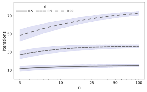
Figure 1: Number of iterations needed for convergence at threshold $\delta=10^{-8}\sqrt{n}$, when $C_{ij}=\rho^{|i-j|}$ $i,j=1,\ldots,n$, for $n=3,\ldots,100$, using random initial value, $x_{(0)}$. Black lines correspond to the average number of iterations required for convergence, and the shaded bands ($\pm$2 standard deviations) show the variation resulting from the different starting values.

The results in Figure 1 are not specific to the Toeplitz structure for $C$. In a second design, we generate 50,000 distinct correlation matrices for each of the dimensions, $n\in\{5,10,25\}$. This is done by generating random vectors, $\gamma$, where each element in $\gamma$ is uniformly distributed on the interval $[-b_{n},b_{n}]$. The constant, $b_{n}$, is chosen to provide a sufficiently wide range of the smallest eigenvalue of $C$, denoted $\lambda_{\min}$, and the spectral radius of $\nabla g(x^{\ast})$, denoted $\nu_{\max}$. The Lipschitz constant for the contraction, $g(x)$, is approximately equal to $\nu_{\max}$, so we should expect $-1/\log\nu_{\max}\simeq c_{L}$ to be linearly related to (the bound on) the number of iterations.

The number of iterations needed for convergence is shown in Figure 2, for $n=5$, $n=10$, and $n=25$, using scatter plots against three characteristics of $C$. The starting value is $x_{(0)}=0\in\mathbb{R}^{n}$ in all simulations and $\delta=10^{-8}\sqrt{n}$ was used as the tolerance level.

The left panels reveal a fairly tight linear relationship between the number of iterations and $-1/\log\nu_{\max}$ ($\approx c_{L}$). Similarly, $\lambda_{\max}$ and $\gamma_{\max}$, which are easier to compute, are also related to the number of iterations, albeit not as tightly as $\nu_{\max}$.

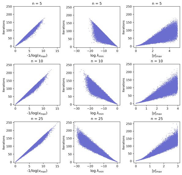
Figure 2: The number of iterations needed for convergence plotted against three characteristics of $C$. The left panels plots the number of iterations against $-1/\log\nu_{\max}\simeq c_{L}$. The smallest eigenvalue of $C$ (middle panels) and the largest $|\gamma_{i}|$ (right panels) are also useful indicators.

6 Concluding Remarks

In this paper, we have shown that the space of non-singular $n\times n$ correlation matrices is one-to-one with $\mathbb{R}^{n(n-1)/2}$. A non-singular covariance matrix can therefore be parametrized by the $n$ (log-)variances and the vector, $\gamma(C)$, which has unrestricted domain in $\mathbb{R}^{n(n-1)/2}$. This opens new ways to model correlation and covariance matrices where positive definiteness is an intrinsic property. For instance, in multivariate GARCH models, as explored in Archakov et al. (2020). The transformation can be used to specify probability distributions on correlation and covariance matrices. Any distribution on $\mathbb{R}^{n(n-1)/2}$ induces a distribution on the space of positive definite correlation matrices, $\mathcal{C}$. This could be used in multivariate stochastic volatility modeling, and defines a new approach to specifying Bayesian priors on $\mathcal{C}$.

We have derived results for the asymptotic distribution of $\gamma(\hat{C})$. Much is known about the finite sample properties when $n=2$, because $\gamma(C)$ is identical to the Fisher transformation in this case. The Fisher transformation has variance stabilizing and skewness eliminating properties. The variance stabilizing property does not carry over to the case $n>2$. However, simulation results suggest that it continues to have skewness reducing properties, and that the empirical distribution of $\gamma(\hat{C})$ (in a classical setting) is well approximated by a Gaussian distribution even in small samples. Moreover, the elements of $\gamma(\hat{C})$ tend to be weakly dependent, as suggested by the asymptotic results in Table 1. This makes the transformation potentially useful for regularization, see Pourahmadi (2011), and inference. These attributes tend to deteriorate as $C$ approaches singularity. This is not unexpected, because it is also true for the Fisher transformation when the correlation is close to $\pm 1$.

The inverse mapping, $C(\gamma)$ is not given in closed-form when $n>2$, except in some special cases. Instead, we proposed a fast algorithm to evaluate $C(\gamma)$, and showed that its numerical complexity is of order $O(n^{3}\log n)$, where $n\times n$ is the dimension of $C$.

Appendix of Proofs

We prove $g$ is a contraction by deriving its Jacobian, $J(x)$, and showing that all its eigenvalues are less than one in absolute value. Since $g(x)=x-\log\delta(x),$ where $\delta(x)=\text{diag}(e^{G[x]})$, an intermediate step towards the Jacobian for $g$, is to derive the Jacobian for $\delta(x)$. To simplify notation, we sometimes suppress the dependence on $x$ for some terms. For instance, we sometimes write $\delta_{i}$ to denote the $i$-th element of the vector $\delta(x)$. It follows that $[J(x)]_{i,j}=\frac{\partial[g(x)]_{i}}{\partial x_{j}}=1_{\{i=j\}}-\frac{1}{\delta_{i}}\frac{\partial[\delta(x)]_{i}}{\partial x_{j}},$ so that $J(x)=I-[D(x)]^{-1}H(x)$, where $D(x)=\mathrm{diag}(\delta_{1},\ldots,\delta_{n})$ is a diagonal matrix and $H(x)$ is the Jacobian matrix of $\delta(x)$, derived below.

Let $G[x]=Q\Lambda Q^{\prime}$, where $\Lambda$ is the diagonal matrix with the eigenvalues, $\lambda_{1},\ldots,\lambda_{n}$, of $G[x]$ and $Q$ is an orthonormal matrix (i.e. $Q^{\prime}=Q^{-1}$) with the corresponding eigenvectors. From Linton & McCrorie (1995), we have $\mathrm{d}\text{vec}\,e^{G[x]}=A(x)\,\mathrm{d}\text{vec}G[x]$, where

$$A(x)=(Q\otimes Q)\Xi\bigl{(}Q\otimes Q\bigl{)}^{\prime},$$ (A.1)

is and $n^{2}\times n^{2}$ matrix and $\Xi$ is the $n^{2}\times n^{2}$ diagonal matrix with elements given by

$$\xi_{ij}=\Xi_{(i-1)n+j,(i-1)n+j}=\begin{cases}e^{\lambda_{i}},&\text{if}\qquad\lambda_{i}=\lambda_{j}\\ \tfrac{e^{\lambda_{i}}-e^{\lambda_{j}}}{\lambda_{i}-\lambda_{j}},&\text{if}\qquad\lambda_{i}\neq\lambda_{j}\end{cases}$$ (A.2)

for $i=1,\ldots,n$ and $j=1,\ldots,n$. Evidently, we have $\xi_{ij}=\xi_{ji}$, for all $i$ and $j$. Moreover, $A(x)$ is a symmetric positive definite matrix, because all the diagonal elements of $\Xi$ are strictly positive.

Our interest concerns $\delta(x)=\text{diag}[e^{G[x]}]$ (a subset of the elements of $\text{vec}[e^{G[x]}]$) so the Jacobian of $\delta(x)$, denoted $H(x)$, is a principal sub-matrix of $A(x)$, defined by the elements $[A(x)]_{l,m}$, $l,m=(i-1)n+i$, for $i=1,\ldots,n$. Thus

$$[H(x)]_{i,j} =\frac{\partial\delta(x)_{i}}{\partial x_{j}}=(e_{i}\otimes e_{i})^{\prime}\bigl{(}Q\otimes Q\bigl{)}\Xi\bigl{(}Q\otimes Q)^{\prime}(e_{j}\otimes e_{j})$$

$$=\bigl{(}e_{i}^{\prime}Q\otimes e_{i}^{\prime}Q\bigl{)}\Xi\bigl{(}Q^{\prime}e_{j}\otimes Q^{\prime}e_{j}\bigl{)}=\bigl{(}Q_{i,.}\otimes Q_{i,.}\bigl{)}\Xi\bigl{(}Q_{j,.}\otimes Q_{j,.}\bigl{)}^{\prime}$$ (A.3)

$$=\sum_{k=1}^{n}\sum_{l=1}^{n}q_{ik}q_{jk}q_{il}q_{jl}\xi_{kl},$$

where $e_{i}$ is a $n\times 1$ unit vector with one at the $i$-th position and zeroes otherwise and $Q_{i,.}$ denotes the $i$-th row of $Q$.

Interestingly, the Jacobian of $g$ is such that $J(x)\iota=0$, so that the vector of ones, $\iota$, is an eigenvector of $J(x)$ associated with the eigenvalue $0$, i.e. $J(x)$ has reduced rank. Because the $i$-th row of $J(x)$ times $\iota$ reads

$$1-\sum_{j=1}^{n}\frac{1}{\delta_{i}}\sum_{k=1}^{n}\sum_{l=1}^{n}q_{ik}q_{jk}q_{il}q_{jl}\xi_{kl}=1-\frac{1}{\delta_{i}}\sum_{k=1}^{n}\sum_{l=1}^{n}q_{ik}q_{il}\xi_{kl}\sum_{j=1}^{n}q_{jk}q_{jl}=1-\frac{1}{\delta_{i}}\sum_{k=1}^{n}q_{ik}^{2}\xi_{kk}=0,$$

due to $\sum_{k=1}^{n}q_{ik}q_{jk}=1_{\{i=j\}}$.

Proof that $g$ is a Contraction: Lemma 1

We now want to prove that the mapping $g(x)$ is a contraction. In order to show this, it is sufficient to demonstrate that all eigenvalues of the corresponding Jacobian matrix $J(x)$ are below one in absolute values for any real vector $x$. First we establish a number of intermediate results.

Lemma A.1.

$(i)$ $e^{y}-y-1>0$ for all $y\neq 0$, and $(ii)$ $1+e^{y}-\frac{2}{y}(e^{y}-1)>0$ for $y\neq 0$.

Proof.

The first and second derivatives of $f(y)=e^{y}-y-1$ show that $f$ is strictly convex with unique minimum, $f(0)=0$, which proves $(i)$. Next we prove $(ii)$. Now let $f(y)=1+e^{y}-\frac{2}{y}(e^{y}-1)$. Its first derivative is given by $f^{\prime}(y)=e^{y}y^{-2}g(y)$, where $g(y)=y^{2}-2y+2-2e^{-y}$, so that $f^{\prime}(y)<0$ for $y<0$ and $f^{\prime}(y)>0$ for $y>0$. Since $\lim_{y\rightarrow 0}f(y)=0$ (by l’Hospital’s rule) the result follows. ∎

From the definition, (A.2), it follows that $\xi_{ij}=\xi_{ii}=\xi_{jj}$ whenever $\lambda_{i}=\lambda_{j}$. When $\lambda_{i}\neq\lambda_{j}$ we have the following results for the elements of $\Xi$:

Lemma A.2.

If $\lambda_{i}<\lambda_{j}$, then $\xi_{ii}<\xi_{ij}<\xi_{jj}$ and $2\xi_{ij}<\xi_{ii}+\xi_{jj}$.

Proof.

From the definition, (A.2), $\xi_{ij}-\xi_{ii}=\tfrac{e^{\lambda_{j}}-e^{\lambda_{i}}}{\lambda_{j}-\lambda_{i}}-e^{\lambda_{i}}=e^{\lambda_{i}}(\tfrac{e^{\lambda_{j}-\lambda_{i}}-1}{\lambda_{j}-\lambda_{i}}-1)=e^{\lambda_{i}}\tfrac{e^{\lambda_{j}-\lambda_{i}}-1-(\lambda_{j}-\lambda_{i})}{\lambda_{j}-\lambda_{i}}>0$, where the numerator is positive by Lemma A.1 ($i$). So are $e^{\lambda_{i}}$ and $\lambda_{j}-\lambda_{i}$, which proves $\xi_{ij}>\xi_{ii}$. Analogously, $\xi_{jj}-\xi_{ij}=e^{\lambda_{j}}-\tfrac{e^{\lambda_{j}}-e^{\lambda_{i}}}{\lambda_{j}-\lambda_{i}}=e^{\lambda_{j}}(1-\tfrac{1-e^{\lambda_{i}-\lambda_{j}}}{\lambda_{j}-\lambda_{i}})=e^{\lambda_{j}}\tfrac{-(\lambda_{i}-\lambda_{j})-1+e^{\lambda_{i}-\lambda_{j}}}{\lambda_{j}-\lambda_{i}}>0$, because all terms are positive, where we again used Lemma A.1 ($i$). Next, $\xi_{ii}+\xi_{jj}-2\xi_{ij}=e^{\lambda_{i}}+e^{\lambda_{j}}-2\tfrac{e^{\lambda_{i}}-e^{\lambda_{j}}}{\lambda_{i}-\lambda_{j}}=e^{\lambda_{i}}(1+e^{\lambda_{j}-\lambda_{i}}-2\tfrac{e^{\lambda_{j}-\lambda_{i}}-1}{\lambda_{j}-\lambda_{i}})>0$, where the inequality follows by Lemma A.1.$ii$, because $\lambda_{i}\neq\lambda_{j}$. ∎

Lemma A.3.

$J(x)$ and $\tilde{J}(x)=I-D^{-\frac{1}{2}}HD^{-\frac{1}{2}}$ have the same eigenvalues, where

$$\tilde{J}(x)=\sum_{k=1}^{n-1}\sum_{l=k}^{n}\varphi_{kl}\Bigl{(}D^{-\frac{1}{2}}u_{kl}u_{kl}^{\prime}D^{-\frac{1}{2}}\Bigl{)},$$

with $u_{kl}=Q_{\cdot,k}\odot Q_{\cdot,l}\in\mathbb{R}^{n}$ and $\varphi_{kl}=\xi_{kk}+\xi_{ll}-2\xi_{kl}$.

Proof.

For a vector $y$ and a scalar $\nu$, $Jy=\nu y\Leftrightarrow\tilde{J}w=\nu w$, where $y=D^{-\frac{1}{2}}w$, because $J=I-D^{-1}H=D^{-\frac{1}{2}}(I-D^{-\frac{1}{2}}HD^{-\frac{1}{2}})D^{\frac{1}{2}}=D^{-\frac{1}{2}}\tilde{J}D^{\frac{1}{2}}$. Next, we turn to the expression for $\tilde{J}$. First, note that $\sum_{k=1}^{n}q_{ik}^{2}\xi_{kk}=\sum_{k=1}^{n}q_{ik}^{2}e^{\lambda_{k}}=Q_{i,\cdot}e^{\Lambda}Q_{i,\cdot}^{\prime}=[e^{Q\Lambda Q^{\prime}}]_{ii}=[e^{G}]_{ii}=\delta_{i}$. So diagonal elements of $\tilde{J}$ are given by

$$\tilde{J}_{ii}=1-\frac{H_{ii}}{\delta_{i}} =\frac{1}{\delta_{i}}\Bigl{(}\sum_{k=1}^{n}q_{ik}^{2}\xi_{kk}-\sum_{k=1}^{n}\sum_{l=1}^{n}q_{ik}^{2}q_{il}^{2}\xi_{kl}\Bigl{)}=\frac{1}{\delta_{i}}\Bigl{(}\sum_{k=1}^{n}q_{ik}^{2}\xi_{kk}-\sum_{k=1}^{n}q_{ik}^{2}q_{ik}^{2}\xi_{kk}-2\sum_{k=1}^{n-1}\sum_{l=k}^{n}q_{ik}^{2}q_{il}^{2}\xi_{kl}\Bigl{)}$$

$$=\frac{1}{\delta_{i}}\Bigl{(}\sum_{k=1}^{n}q_{ik}^{2}\xi_{kk}(1-q_{ik}^{2})-2\sum_{k=1}^{n-1}\sum_{l=k}^{n}q_{ik}^{2}q_{il}^{2}\xi_{kl}\Bigl{)}=\frac{1}{\delta_{i}}\Bigl{(}\sum_{k=1}^{n}q_{ik}^{2}\xi_{kk}\sum_{\begin{subarray}{c}l=1\\ l\neq k\end{subarray}}^{n}q_{il}^{2}-2\sum_{k=1}^{n-1}\sum_{l=k}^{n}q_{ik}^{2}q_{il}^{2}\xi_{kl}\Bigl{)}$$

$$=\frac{1}{\delta_{i}}\Bigl{(}\sum_{k=1}^{n-1}\sum_{l=k}^{n}q_{ik}^{2}q_{il}^{2}(\xi_{kk}+\xi_{ll})-2\sum_{k=1}^{n-1}\sum_{l=k}^{n}q_{ik}^{2}q_{il}^{2}\xi_{kl}\Bigl{)}=\frac{1}{\delta_{i}}\sum_{k=1}^{n-1}\sum_{l=k}^{n}q_{ik}^{2}q_{il}^{2}\varphi_{kl},$$

where we used (A.3). Similarly for the off-diagonal elements we have

$$\tilde{J}_{ij}=-\frac{H_{ij}}{\sqrt{\delta_{i}\delta_{j}}} =-\frac{1}{\sqrt{\delta_{i}\delta_{j}}}\sum_{k=1}^{n}\sum_{l=1}^{n}q_{ik}q_{jk}q_{il}q_{jl}\xi_{kl}=-\frac{1}{\sqrt{\delta_{i}\delta_{j}}}\Bigl{(}\sum_{k=1}^{n}q_{ik}^{2}q_{jk}^{2}\xi_{kk}+2\sum_{k=1}^{n-1}\sum_{l=k}^{n}q_{ik}q_{jk}q_{il}q_{jl}\xi_{kl}\Bigl{)}$$

$$=-\frac{1}{\sqrt{\delta_{i}\delta_{j}}}\Bigl{(}\sum_{k=1}^{n}q_{ik}q_{jk}\Big{(}-\sum_{\begin{subarray}{c}l=1\\ l\neq k\end{subarray}}^{n}q_{il}q_{jl}\Big{)}\xi_{kk}+2\sum_{k=1}^{n-1}\sum_{l=k}^{n}q_{ik}q_{jk}q_{il}q_{jl}\xi_{kl}\Bigl{)}$$

$$=-\frac{1}{\sqrt{\delta_{i}\delta_{j}}}\Bigl{(}-\sum_{k=1}^{n-1}\sum_{l=k}^{n}q_{ik}q_{jk}q_{il}q_{jl}(\xi_{kk}+\xi_{ll})+2\sum_{k=1}^{n-1}\sum_{l=k}^{n}q_{ik}q_{jk}q_{il}q_{jl}\xi_{kl}\Bigl{)}$$

$$=\frac{1}{\sqrt{\delta_{i}\delta_{j}}}\sum_{k=1}^{n-1}\sum_{l=k}^{n}q_{ik}q_{jk}q_{il}q_{jl}\varphi_{kl}.$$

In the derivations above we used that $\sum_{k=1}^{n}q_{ik}q_{jk}=1_{\{i=j\}}$, since $Q^{\prime}Q=QQ^{\prime}=I$. ∎

Proof of Lemma 1. Because $A(x)$ is symmetric and positive definite, then so is the principal sub-matrix, $H(x)$. Consequently, $M=D^{-\frac{1}{2}}H(x)D^{-\frac{1}{2}}$ is symmetric and positive definite. Thus, any eigenvalue, $\mu$ of $M$ is strictly positive. So if $\nu$ is an eigenvalue of $\tilde{J}(x)=I-D^{-\frac{1}{2}}HD^{-\frac{1}{2}}$, then $\nu=1-\mu$ where $\mu$ is an eigenvalue of $M$, from which it follows that all eigenvalues of $\tilde{J}$ are strictly less than 1.

Consider a quadratic form of $\tilde{J}$ with an arbitrary vector $z\in\mathbb{R}^{n}$. Using Lemma A.3, it follows that any quadratic form is bounded from below by

$$z^{\prime}\tilde{J}z=\sum_{k=1}^{n-1}\sum_{l=k}^{n}\varphi_{kl}\Bigl{(}z^{\prime}D^{-\frac{1}{2}}u_{kl}u_{kl}^{\prime}D^{-\frac{1}{2}}z\Bigl{)}=\sum_{k=1}^{n-1}\sum_{l=k}^{n}\varphi_{kl}\Bigl{(}z^{\prime}D^{-\frac{1}{2}}u_{kl}\Bigl{)}^{2}\geq 0,$$

because $\varphi_{kl}>0$ by Lemma A.2. Hence, $\tilde{J}$ is positive semi-definite and $\nu_{i}\geq 0$, for all $i=1,\ldots,n$.

Finally, since $J(x)$ and $\tilde{J}(x)$ have the same eigenvalues, it follows that all eigenvalues of $J(x)$ lie within the interval $[0,1)$, which proves that $g(x)$ is a contraction. $\square$

Proof of Theorem 1. The Theorem is equivalent to the statement that for any symmetric matrix $G$, there always exists a unique solution to $g(x)=x$. This follows from Lemma 1 and Banach’s fixed point theorem. $\square$

Proof of Proposition 1. We have $Y=PX$, for some permutation matrix, $P$, so that $C_{y}=PC_{x}P^{\prime}$. Let $C_{x}=Q\Lambda Q^{\prime}$ be the spectral decomposition of $C_{x}$, such that $\log C_{x}=Q\log\Lambda_{x}Q^{\prime}$, where $Q^{\prime}Q=I$ and $\Lambda$ is a diagonal matrix. So $C_{y}=PC_{x}P^{\prime}=PQ\Lambda Q^{\prime}P^{\prime}$, where $Q^{\prime}P^{\prime}PQ=Q^{\prime}Q=I$. The first equality uses the fact that $P$ is a permutation matrix. Therefore, $C_{y}=(PQ)\Lambda(PQ)^{\prime}$ is the spectral decomposition of $C_{y}$ and $\log C_{y}=(PQ)\log\Lambda(PQ)^{\prime}=P[\log C_{x}]P^{\prime}$.

Next, let the $i$-th and $j$-th rows of $P$ be the $r$-th and $s$-th unit vectors, $e_{r}^{\prime}$ and $e_{s}^{\prime}$, respectively. Then we have $[\log C_{y}]_{ij}=[\log C_{x}]_{rs}$ and, by symmetry,

$$[\log C_{y}]_{ij}=[\log C_{y}]_{ji}=[\log C_{x}]_{rs}\mathbf{=}[\log C_{x}]_{sr},$$

which shows that $\gamma_{y}$ is simply a permutation of the elements in $\gamma_{x}$. $\square$

Proof of Proposition 2. An equicorrelation matrix can be written as $C=(1-\rho)I_{n}+\rho U_{n}$, where $I_{n}\in\mathbb{R}^{n\times n}$ is the identity matrix and $U_{n}\in\mathbb{R}^{n\times n}$ is a matrix of ones. Using the Sherman–Morrison formula, we can obtain the inverse, $C^{-1}=\frac{1}{1-\rho}(I_{n}-\frac{\rho}{1+(n-1)\rho}U_{n})$, so that

$$G=\log C=-\log(C^{-1})=-\log(\tfrac{1}{1-\rho}I_{n})-\log(I_{n}-\tfrac{\rho}{1+(n-1)\rho}U_{n}).$$ (A.4)

Because the first term is a diagonal matrix, the off-diagonal elements of $G$ are determined only by the second term, which equals

$$-\log(I_{n}-\varphi U_{n})=-\sum_{k=1}^{\infty}(-1)^{k+1}\tfrac{(-\varphi U_{n})^{k}}{k}=-\left[\frac{1}{n}\sum_{k=1}^{\infty}(-1)^{k+1}\tfrac{(-n\varphi)^{k}}{k}\right]U_{n}=-\frac{1}{n}\log(1-n\varphi)U_{n},$$ (A.5)

where $\varphi=\rho/(1+(n-1)\rho)$ and we have used the fact that $U_{n}^{k}=n^{k-1}U_{n}$. It now follows that

$$G_{ij}=\gamma_{c}=-\frac{1}{n}\log(1-\tfrac{n\rho}{1+(n-1)\rho})=-\frac{1}{n}\log\tfrac{1-\rho}{1+\rho(n-1)}=-\frac{1}{n}\log\tfrac{1-\rho}{1+\rho(n-1)},\quad\text{for all }i\neq j$$

for all $i$ and $j$, such that $i\neq j$. $\square$

Proof of Proposition 3. From Theorem 1 it follows that the diagonal, $x=\mathrm{diag}G$, is fully characterized by the off-diagonal elements, $y=\mathrm{vecl}G=\mathrm{vecl}G^{\prime}$, and we may write $x=x(y)$. For the off-diagonal elements of the correlation matrix, $z=\mathrm{vecl}C\mathrm{=vecl}C^{\prime}$, we have $z=z(x,y)=z(x(y),y)$, since $C=e^{G}$, and it follows that

$$\frac{dz(x,y)}{dy}=\frac{\partial z(x,y)}{\partial x}\frac{dx(y)}{dy}+\frac{\partial z(x,y)}{\partial y}.$$ (A.6)

With $A(x,y)=d\mathrm{vec}C/d\mathrm{vec}G$ and the definitions of $E_{l}$ and $E_{u}$, the second term is given by:

$$\frac{\partial z(x,y)}{\partial y}=E_{l}A(x,y)E_{l}^{\prime}+E_{l}A(x,y)E_{u}^{\prime}.$$ (A.7)

The expression has two terms because a change in an element of $y$ affects two symmetric entries in the matrix $G$. Similarly, for the first part of the first term in (A.6) we have,

$$\frac{\partial z(x,y)}{\partial x}=E_{l}A(x,y)E_{d}^{\prime},$$ (A.8)

and what remains is to determine $\frac{dx(y)}{dy}$. For this purpose we introduce $D(x,y)=\mathrm{diag}[e^{G(x,y)}]-\iota$ which implicitly defines the relation between $x$ and $y$. The requirement that $e^{G}$ is a correlation matrix, is equivalent to $D(x,y)=0$. Next, let $\frac{\partial D}{\partial x}$ and $\frac{\partial D}{\partial y}$ denote the Jacobian matrices of $D(x,y)$ with respect to $x$ and $y$, respectively. These Jacobian matrices have dimensions $n\times n$ and $n\times n(n-1)/2$, respectively, and can also be expressed in terms of matrix $A(x,y)$, as follows

$$\frac{\partial D}{\partial x}=E_{d}A(x,y)E_{d}^{\prime}, \qquad\frac{\partial D}{\partial y}=E_{d}A(x,y)E_{l}^{\prime}+E_{d}A(x,y)E_{u}^{\prime}.$$

Note that $\frac{\partial D}{\partial x}$ is a principal sub-matrix of positive definite matrix $A$ and, hence, is an invertible matrix. Therefore, from the Implicit Function Theorem it follows

$$\frac{dx(y)}{dy}=-\Bigl{(}\frac{\partial D}{\partial x}\Bigl{)}{}^{-1}\frac{\partial D}{\partial y}=-\Bigl{(}E_{d}A(x,y)E_{d}^{\prime}\Bigl{)}{}^{-1}\Bigl{(}E_{d}A(x,y)E_{l}^{\prime}+E_{d}A(x,y)E_{u}^{\prime}\Bigl{)}.$$ (A.9)

The results now follows by inserting (A.7), (A.8) and (A.9) into (A.6). $\square$

Proof of Lemma 2. We have $G=Q\log\Lambda Q^{\prime}$, where $C=Q\Lambda Q^{\prime}$ is the spectral decomposition of the correlation matrix. Thus a generic element of $G$ can be written as $G_{ij}=\sum_{k=1}^{n}q_{ik}q_{jk}\log\lambda_{k}$. By Jensen’s inequality it follows that $G_{ii}=\sum_{k=1}^{n}q_{ik}^{2}\log\lambda_{k}\leq\log\left(\sum_{k=1}^{n}q_{ik}^{2}\lambda_{k}\right)$, where we used that $\sum_{k=1}^{n}q_{ik}q_{jk}=1_{\{i=j\}}$, because $Q^{\prime}Q=I$. Finally, since $\sum_{k=1}^{n}q_{ik}^{2}\lambda_{k}=C_{ii}=1$, it follows that $G_{ii}\leq\log 1=0$. $\square$

References

• (1)
• Archakov & Hansen (2020) Archakov, I. & Hansen, P. R. (2020), ‘Web-appendix for: A New Parametrization of Correlation Matrices’, https://sites.google.com/site/peterreinhardhansen/ .
• Archakov et al. (2020) Archakov, I., Hansen, P. R. & Lunde, A. (2020), ‘A Multivariate Realized GARCH Model’, Working Paper .
• Asai & So (2015) Asai, M. & So, M. (2015), ‘Long memory and asymmetry for matrix-exponential dynamic correlation processes’, Journal of Time Series Econometrics 7, 69–74.
• Bauer & Vorkink (2011) Bauer, G. H. & Vorkink, K. (2011), ‘Forecasting multivariate realized stock market volatility’, Journal of Econometrics 160, 93–101.
• Bauwens et al. (2012) Bauwens, L., Storti, G. & Violante, F. (2012), ‘Dynamic conditional correlation models for realized covariance matrices’, Working Paper (2012060).
• Bollerslev (1990) Bollerslev, T. (1990), ‘Modelling the coherence in short-run nominal exchange rates: A multivariate generalized ARCH model’, The Review of Economics and Statistics 72, 498–505.
• Browne & Shapiro (1986) Browne, M. & Shapiro, A. (1986), ‘The asymptotic covariance matrix of sample correlation coefficients under general conditions’, Linear Algebra and its Applications 82, 169 – 176.
• Chiriac & Voev (2011) Chiriac, R. & Voev, V. (2011), ‘Modelling and forecasting multivariate realized volatility’, Journal of Applied Econometrics 26, 922–947.
• Chiu et al. (1996) Chiu, T., Leonard, T. & Tsui, K.-W. (1996), ‘The matrix-logarithmic covariance model’, Journal of the American Statistical Association 91, 198–210.
• Creal et al. (2013) Creal, D. D., Koopman, S. J. & Lucas, A. (2013), ‘Generalized autoregressive score models with applications’, Journal of Applied Econometrics 28, 777–795.
• Engle (2002) Engle, R. F. (2002), ‘Dynamic Conditional Correlation: A Simple Class of Multivariate Generalized Autoregressive Conditional Heteroskedasticity Models’, Journal of Business & Economic Statistics 20(3), 339–350.
• Engle & Kelly (2012) Engle, R. & Kelly, B. (2012), ‘Dynamic Equicorrelation’, Journal of Business & Economic Statistics 30(2), 212–228.
• Golosnoy et al. (2012) Golosnoy, V., Gribisch, B. & Liesenfeld, R. (2012), ‘The conditional autoregressive Wishart model for multivariate stock market volatility’, Journal of Econometrics 167(1), 211–223.
• Gorgi et al. (2019) Gorgi, P., Hansen, P. R., Janus, P. & Koopman, S. J. (2019), ‘Realized Wishart-GARCH: A score-driven multi-asset volatility model’, Journal of Financial Econometrics 17, 1–32.
• Hansen et al. (2014) Hansen, P. R., Lunde, A. & Voev, V. (2014), ‘Realized beta GARCH: A multivariate GARCH model with realized measures of volatility’, Journal of Applied Econometrics 29, 774–799.
• Higham (2008) Higham, N. J. (2008), Functions of Matrices: Theory and Computation, Siam, Philadelphia.
• Ishihara et al. (2016) Ishihara, T., Omori, Y. & Asai, M. (2016), ‘Matrix exponential stochastic volatility with cross leverage’, Computational Statistics & Data Analysis 100, 331–350.
• Kawakatsu (2006) Kawakatsu, H. (2006), ‘Matrix exponential GARCH’, Journal of Econometrics 134, 95–128.
• Kurowicka & Cooke (2003) Kurowicka, D. & Cooke, R. (2003), ‘A parameterization of positive definite matrices in terms of partial correlation vines’, Linear Algebra and Its Applications 372, 225–251.
• Leonard & Hsu (1992) Leonard, T. & Hsu, J. S. J. (1992), ‘Bayesian inference for a covariance matrix’, Annals of Statistics 20, 1669–1696.
• Linton & McCrorie (1995) Linton, O. & McCrorie, J. R. (1995), ‘Differentiation of an exponential matrix function: Solution’, Econometric Theory 11, 1182–1185.
• Liu (2009) Liu, Q. (2009), ‘On portfolio optimization: How and when do we benefit from high-frequency data?’, Journal of Applied Econometrics 24(4), 560–582.
• Lu (1998) Lu, Y. Y. (1998), ‘Exponential of symmetric matrices though tridiagonal reductions’, Linear Algebra and its Applications 279, 317–324.
• Nel (1985) Nel, D. (1985), ‘A matrix derivation of the asymptotic covariance matrix of sample correlation coefficients’, Linear Algebra and its Applications 67, 137 – 145.
• Neudecker & Wesselman (1990) Neudecker, H. & Wesselman, A. (1990), ‘The asymptotic variance matrix of the sample correlation matrix’, Linear Algebra and its Applications 127, 589 – 599.
• Noureldin et al. (2012) Noureldin, D., Shephard, N. & Sheppard, K. (2012), ‘Multivariate high-frequency-based volatility (HEAVY) models’, Journal of Applied Econometrics 27, 907–933.
• Nyblom (1989) Nyblom, J. (1989), ‘Testing for the constancy of parameters over time’, Journal of the American Statistical Association 84, 223–230.
• Pinheiro & Bates (1996) Pinheiro, J. C. & Bates, D. M. (1996), ‘Unconstrained parametrizations for variance-covariance matrices’, Statistics and Computing 6, 289–296.
• Pourahmadi (2011) Pourahmadi, M. (2011), ‘Covariance estimation: The glm and regularization perspectives’, Statistical Science 26, 369–387.
• Tse & Tsui (2002) Tse, Y. K. & Tsui, A. K. C. (2002), ‘A multivariate generalized autoregressive conditional heteroscedasticity model with time-varying correlations’, Journal of Business and Economic Statistics 20, 351–362.
• Weigand (2014) Weigand, R. (2014), ‘Matrix Box-Cox models for multivariate realized volatility’, Working Paper .