Local Number Fluctuations in Hyperuniform and Nonhyperuniform Systems: Higher-Order Moments and Distribution Functions

Abstract

The local number variance $\sigma^{2}(R)$ associated with a spherical sampling window of radius $R$ enables a classification of many-particle systems in $d$-dimensional Euclidean space $\mathbb{R}^{d}$ according to the degree to which large-scale density fluctuations are suppressed, resulting in a demarcation between hyperuniform and nonhyperuniform phyla. To more completely characterize density fluctuations, we carry out an extensive study of higher-order moments or cumulants, including the skewness $\gamma_{1}(R)$, excess kurtosis $\gamma_{2}(R)$ and the corresponding probability distribution function $P[N(R)]$ of a large family of models across the first three space dimensions, including both hyperuniform and nonhyperuniform systems with varying degrees of short- and long-range order. To carry out this comprehensive program, we derive new theoretical results that apply to general point processes and conduct high-precision numerical studies. Specifically, we derive explicit closed-form integral expressions for $\gamma_{1}(R)$ and $\gamma_{2}(R)$ that encode structural information up to three-body and four-body correlation functions, respectively. We also derive rigorous bounds on $\gamma_{1}(R)$, $\gamma_{2}(R)$ and $P[N(R)]$ for general point processes and corresponding exact results for general packings of identical spheres. High-quality simulation data for $\gamma_{1}(R)$, $\gamma_{2}(R)$ and $P[N(R)]$ are generated for each model. We also ascertain the proximity of $P[N(R)]$ to the normal distribution via a novel Gaussian “distance” metric $l_{2}(R)$. Among all models, the convergence to a central limit theorem (CLT) is generally fastest for the disordered hyperuniform processes such that $\gamma_{1}(R)\sim l_{2}(R)\sim R^{-(d+1)/2}$ and $\gamma_{2}(R)\sim R^{-(d+1)}$ for large $R$. The convergence to a CLT is slower for standard nonhyperuniform models and slowest for the “antihyperuniform” model studied here. We prove that one-dimensional hyperuniform systems of class I or any $d$-dimensional lattice cannot obey a CLT. Remarkably, we discovered that the gamma distribution provides a good approximation to $P[N(R)]$ for all models that obey a CLT across all dimensions for intermediate to large values of $R$, enabling us to estimate the large-$R$ scalings of $\gamma_{1}(R)$, $\gamma_{2}(R)$ and $l_{2}(R)$. For any $d$-dimensional model that “decorrelates” or “correlates” with $d$, we elucidate why $P[N(R)]$ increasingly moves toward or away from Gaussian-like behavior, respectively. Our work elucidates the fundamental importance of higher-order structural information to fully characterize density fluctuations in many-body systems across length scales and dimensions, and thus has broad implications for condensed matter physics, engineering, mathematics and biology.

I Introduction

The quantification of density fluctuations in many-particle systems in $d$-dimensional Euclidean space $\mathbb{R}^{d}$ is of great fundamental and practical importance in many fields across the physical, mathematical and biological sciences Schofield (1966); Vezzetti (1975); Ziff (1977); Carmona and Delhaes (1978); Hansen and McDonald (1986); Jørgensen et al. (1991); Peebles (1993); Bleher et al. (1993); Truskett et al. (1998); Torquato (2000); Gabrielli et al. (2002); Wax et al. (2002); Torquato and Stillinger (2003); Lavery et al. (2003); Klatt and Torquato (2016); Torquato (2018a). It is well known that long-wavelength density fluctuations of disordered as well as ordered systems contain crucial information about the structure as well as equilibrium and nonequilibrium physical properties of the systems Schofield (1966); Hansen and McDonald (1986); Torquato and Stillinger (2003); Torquato (2018a). Clearly, density fluctuations that occur on some arbitrary local length scale Vezzetti (1975); Ziff (1977); Bleher et al. (1993); Truskett et al. (1998); Román et al. (1999); Gabrielli et al. (2002); Wax et al. (2002); Torquato and Stillinger (2003); Klatt and Torquato (2016); Torquato (2018a); Zheng and Ciamarra (2020) provide considerably more information about the system than those in the long-wavelength limit.

Consider a statistically homogeneous (translationally invariant) point process in $d$-dimensional Euclidean space $\mathbb{R}^{d}$ at number density $\rho$ and sampling for the number of points $N(R)$ within a $d$-dimensional spherical window of radius $R$ (see Fig. 1) and volume

$$v_{1}(R)=\frac{\pi^{d/2}R^{d}}{\Gamma(1+d/2)}.$$ (1)

The local number variance $\sigma^{2}(R)\equiv\langle N^{2}(R)\rangle-\langle N(R)\rangle^{2}$ is a useful measure of number fluctuations, where the first moment $\langle N(R)\rangle=\rho v_{1}(R)$ is the average number of points within a $d$-dimensional spherical (sampling) window of radius $R$ and angular brackets denote an ensemble average. The local number variance is exactly determined by pair statistics, and can be given either in terms of the pair correlation function $g_{2}({\bf r})$ in direct space or the structure factor $S({\bf k})$ in reciprocal space Torquato and Stillinger (2003):

$$\sigma^{2}(R) = \rho v_{1}(R)\left[1+\rho\int_{\mathbb{R}^{d}}h({\bf r})\alpha_{2}(r;R)\,d{\bf r}\right],$$ (2)

$$= \rho v_{1}(R)\Big{[}\frac{1}{(2\pi)^{d}}\int_{\mathbb{R}^{d}}S({\bf k}){\tilde{\alpha}}_{2}(k;R)d{\bf k}\Big{]},$$ (3)

where $h({\bf r})\equiv g_{2}({\bf r})-1$ is the total correlation function, $\alpha_{2}(r;R)$ is the intersection volume of two spherical windows of radius $R$, scaled by $v_{1}(R)$, whose centers are separated by the distance $r$, and ${\tilde{\alpha}}_{2}(k;R)$ is its Fourier transform. The large-scale behavior of the number variance $\sigma^{2}(R)$ is central to the hyperuniformity concept, which is attracting attention across many fields Torquato and Stillinger (2003); Torquato (2018a); Chremos and Douglas (2018); Zheng (2020); Sheremet et al. (2020); Wilken et al. (2020); Ma et al. (2020). Specifically, a hyperuniform point process is one in which $\sigma^{2}(R)$ grows slower than the window volume, i.e., $R^{d}$, for large $R$ and hence is characterized by large-scale density fluctuations that are anomalously suppressed compared to those of typical disordered systems. The hyperuniformity concept generalizes the traditional notion of long-range order of crystals and quasicrystals to also encompass certain exotic disordered states of matter Torquato and Stillinger (2003); Torquato (2018a). Disordered hyperuniform systems are diametrically opposite to systems at thermal critical points in which the local variance diverges faster than $R^{d}$ in the limit $R\to\infty$. Any system with such divergent behavior in the local variance has been called anti-hyperuniform Torquato (2018a) (see also Sec. II for additional details).

While the local number variance contains useful information, one would like to more completely characterize the fluctuations by ascertaining higher-order moments, i.e., $\langle N^{k}(R)\rangle$, where $k\geq 3$, as well as the corresponding discrete probability distribution $P[N(R)]$ associated with finding exactly $N(R)$ particles within a $d$-dimensional spherical window of radius $R$. The $m$th moment of the distribution is given by

$$\langle N^{m}(R)\rangle=\sum_{N(R)=0}N^{m}(R)P[N(R)].$$ (4)

Due to the fact that the random variable $N(R)$ is discrete and cannot take on negative values, the probability distribution $P[N(R)]$, for finite $R$, can never exactly attain the normal distribution, which is given by

$$P[N(R)]=\frac{1}{\sqrt{2\pi}\sigma(R)}\exp[\frac{(N(R)-\langle N(R)\rangle)^{2}}{2\sigma^{2}(R)}].$$ (5)

For example, for a statistically homogeneous Poisson point process in $\mathbb{R}^{d}$ at number density $\rho$,

$$P[N(R)]=\frac{[\rho v_{1}(R)]^{N(R)}}{N(R)!}\exp[-\rho v_{1}(R)],$$ (6)

which deviates significantly from the normal distribution for sufficiently small $R$. This is one of the rare cases in which a closed-form analytic formula for $P[N(R)]$ is known across dimensions for nontrivial point processes. It is only when $R$ tends to infinity that the Poisson distribution becomes a normal distribution, i.e., it follows a central limit theorem (CLT); see Ref. Last and Penrose (2017) and references therein. The reader is referred to Refs. Penrose and Yukich (2002); Heinrich et al. (2006); Schreiber and Yukich (2013); Błaszczyszyn et al. (2019) for proofs of CLT for other point processes.

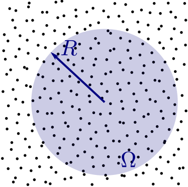
Figure 1: Schematic showing a spherical window $\Omega$ of radius $R$ used to sample fluctuations in the number of points in a two-dimensional point process.

In this paper, we investigate the skewness $\gamma_{1}(R)$ (related to the first three moments), excess kurtosis $\gamma_{2}(R)$ (related to the first four moments), and the number distribution function $P[N(R)]$ for general homogeneous point processes in $\mathbb{R}^{d}$ as well as a wide class of models across dimensions. Specifically, we derive explicit closed-form integral expressions for $\gamma_{1}(R)$ in terms of the number density $\rho$, the pair correlation function $g_{2}$ and the three-body correlation function $g_{3}$ (defined in Sec. II). Similarly, we derive corresponding formulas for the excess kurtosis $\gamma_{2}(R)$, which now depends additionally on the four-body correlation function $g_{4}$. These integral relations also involve geometrical information about the spherical windows via the intersection volumes of up to three and four spheres in the cases of the skewness and excess kurtosis, respectively. Thus, the skewness and excess kurtosis encode up to three-body and four-body information about spatial correlations and window geometries, respectively. We also derive some exact elementary results for the skewness, excess kurtosis and number distribution that apply to general packings of identical spheres.

Via high-precision computer simulation studies, we accurately determine the number variance, skewness, excess kurtosis and the number distribution for up to eight different models of statistically homogeneous point processes across the first three space dimensions and wide range of window radii $R$. These models include both nonhyperuniform and hyperuniform systems with varying degrees of short- and long-range order. Among the nonhyperuniform point processes, we characterize fluctuations of Poisson, random sequential addition (RSA) packings, equilibrium hard spheres, Poisson cluster and anti-hyperuniform point processes. Among the hyperuniform point processes, we characterize hypercubic lattices, randomly perturbed lattices, and stealthy disordered hyperuniform systems. We show that our simulation results for $\gamma_{1}(R)$, $\gamma_{2}(R)$ and $P[N(R)]$ for all models are in excellent agreement with the aforementioned rigorous bounds and exact results for the applicable ranges of $R$. For all disordered hyperuniform models, our explicit general formulas of these quantities in terms of $n$-body information enable us to infer the existence of “hidden” order that manifests itself for the first time at the three-body level or higher.

For each model considered in this paper, we are interested in ascertaining how large $R$ must be such that $P[N(R)]$ is well-approximated by the Gaussian (normal) distribution. We have found that such “distance” metrics proposed previously are not adequate for assessing the diverse set of models that we consider here across dimensions. We quantify this proximity to the normal distribution for any model by introducing a certain Gaussian “distance” metric $l_{2}(R)$, defined in Sec. VII. This distance metric enables us to accurately determine when the distribution function $P[N(R)]$ for a particular model is tending to a CLT. Because the distributions for all models (except the lattices) across dimensions are unimodal, the tendency to a CLT corresponds to the skewness and excess kurtosis simultaneously tending to zero. We have found that almost all of the considered models across dimensions obey a CLT. The convergence to a CLT is slowest for the anti-hyperuniform point process, followed by the Poisson cluster process, and the Poisson process. The nonhyperuniform RSA and equilibrium packings tend to a CLT at the same rate as a Poisson point process but with smaller coefficients of proportionality. Among all models, the convergence to a CLT is generally fastest for the disordered hyperuniform processes. The only models considered that do not achieve a CLT are the hypercubic lattices for any $d$ and 1D hyperuniform systems of class I. The reader is referred to Sec. VII for details.

We have examined a variety of well-known closed-form probability distributions $P[N(R)]$ to ascertain those which best approximate the actual distributions for finite $R$ for all of our models. Interestingly, the gamma distribution provides a good approximation to the number distribution $P[N(R)]$ for all models that obey a CLT across all dimensions for intermediate to large values of $R$ (Sec. VII.3). It is noteworthy that the approximation of $P[N(R)]$ by a gamma distribution enables us to estimate the large-$R$ scalings of $\gamma_{1}(R)$, $\gamma_{2}(R)$ and $l_{2}(R)$ for all models across dimensions that obey a CLT. Among all models, the convergence to a CLT is generally fastest for the disordered hyperuniform processes such that $\gamma_{1}(R)\sim l_{2}(R)\sim R^{-(d+1)/2}\text{~{}and~{}}\gamma_{2}(R)\sim R^{-(d+1)}$ for large $R$. For standard nonhyperuniform models, convergence to a CLT is slower such that $\gamma_{1}(R)\sim l_{2}(R)\sim R^{-d/2}\text{~{}and~{}}\gamma_{2}(R)\sim R^{-d}$. Finally, convergence to a CLT is slowest for the antihyperuniform model such that $\gamma_{1}(R)\sim l_{2}(R)\sim R^{-1/2}\text{~{}and~{}}\gamma_{2}(R)\sim R^{-1}$. These predictions are corroborated by corresponding simulation results.

An important fundamental question is what is the effect of increasing the space dimension on number fluctuations for any particular model? To answer this question, we recall the so-called decorrelation principle Torquato and Stillinger (2006a), which roughly states that for any disordered point process, unconstrained correlations that exist in low dimensions vanish as $d$ tends to infinity, and all higher-order correlation functions $g_{n}$ for $n\geq 3$ may be expressed in terms of the number density $\rho$ and pair correlation function $g_{2}$. The decorrelation principle was employed to justify the conjecture that the densest sphere packings in sufficiently high dimensions are disordered (as opposed to ordered in low dimensions) Torquato and Stillinger (2006a); Scardicchio et al. (2008). Importantly, decorrelation in pair statistics has been shown to manifest itself in low dimensions in the case of disordered sphere packings Skoge et al. (2006); Torquato and Stillinger (2006b); Torquato et al. (2006) as well as other disordered systems with strongly repulsively interacting particles Torquato et al. (2008); Zachary et al. (2008). Since the number distribution function $P[N(R)]$ generally involves certain integrals over all of the $n$-body correlation functions, the decorrelation principle implies that $P[N(R)]$ increasingly becomes Gaussian-like as the space dimension increases for any model that decorrelates with $d$. Similarly, for models the correlate with $d$, $P[N(R)]$ increasingly deviates from the normal distribution as $d$ increases. We confirm such behaviors for all models that obey a CLT (Sec. VII.4).

In Sec. II, we provide basic definitions and necessary background material. In Sec. III, we derive explicit closed-form integral expressions for $\gamma_{1}(R)$ and $\gamma_{2}(R)$ as well as rigorous lower bounds on both of these quantities. We also obtain some general exact results for the first few cumulants and distribution functions for sphere packings, whether disordered or not. Section IV describes the large variety of nonhyperuniform and hyperuniform models in one, two and three dimensions that we study in this paper. In Sec. V, we discuss our proposed Gaussian distance metric. Section VI describes the simulation procedure that we employ to sample the first four cumulants and number distributions. In Sec. VII, we present our results. We make concluding remarks in Sec. VIII.

II Definitions and Background

A stochastic point process in $\mathbb{R}^{d}$ is defined as a mapping from a probability space to configurations of points ${\bf r}_{1},{\bf r}_{2},{\bf r}_{3}\ldots$ in $d$-dimensional Euclidean space $\mathbb{R}^{d}$; see Ref. Chiu et al. (2013) for mathematical details. Let $X$ denote the set of configurations such that each configuration $x\in X$ is a subset of $\mathbb{R}^{d}$ that satisfies two regularity conditions: (i) there are no multiple points (${\bf r}_{i}\neq{\bf r}_{j}$ if $i\neq j$) and (ii) each bounded subset of $\mathbb{R}^{d}$ must contain only a finite number of points of $x$ (i.e.,, $x$ is “locally finite”). The point process is statistically is characterized by the generic $n$-particle probability density function $\rho_{n}({\bf r}^{n})$, where ${\bf r}^{n}$ is a shorthand notation for the position vectors of any $n$ points, i.e., ${\bf r}^{n}\equiv{\bf r}_{1},{\bf r}_{2},\ldots,{\bf r}_{n}$ Hansen and McDonald (1986); Torquato (2002). In words, the quantity $\rho_{n}({\bf r}^{n})d{\bf r}^{n}$ is proportional to the probability of finding any $n$ particles with configuration $\bf r^{n}$ in volume element $d{\bf r}^{n}\equiv d{\bf r}_{1}d{\bf r}_{2}\cdots d{\bf r}_{n}$, i.e., it is the probability measure. For any subvolume $\Omega\in\mathbb{R}^{d}$, the following normalization (average) condition involving the fluctuating number of particles within this subvolume, $N_{\Omega}$, immediately follows

$$\left\langle\frac{N_{\Omega}!}{(N_{\Omega}-n)!}\right\rangle_{\Omega}=\int_{\Omega}\int_{\Omega}\cdots\int_{\Omega}\rho_{n}({\bf r}^{n})d{\bf r}^{n},$$ (7)

Note that this random setting is quite general; it incorporates cases in which the locations of the points are deterministically known, such as a lattice.

For statistically homogeneous media, $\rho_{n}({\bf r}^{n})$ is translationally invariant and hence depends only on the relative displacements, say with respect to ${\bf r}_{1}$:

$$\rho_{n}({\bf r}^{n})=\rho_{n}({\bf r}_{12},{\bf r}_{13},\ldots,{\bf r}_{1n}),$$ (8)

where ${\bf r}_{ij}={\bf r}_{j}-{\bf r}_{i}$. In particular, the one-particle function $\rho_{1}$ is just equal to the constant number density of particles $\rho$. For statistically homogeneous point patterns, it is convenient to define the so-called $n$-particle correlation function

$$g_{n}({\bf r}^{n})=\frac{\rho_{n}({\bf r}^{n})}{\rho^{n}}.$$ (9)

In systems without long-range order and in which the particles are mutually far from one another, $\rho_{n}({\bf r}^{n})\rightarrow\rho^{n}$ and we have from (9) that $g_{n}({\bf r}^{n})\rightarrow 1$. Thus, the deviation of $g_{n}$ from unity provides a measure of the degree of spatial correlation between the particles, with unity corresponding to no spatial correlation.

The important two-particle quantity $g_{2}({\bf r}_{12})$ is usually referred to as the pair correlation function. The total correlation function $h({\bf r}_{12})$ is defined as

$$h({\bf r}_{12})=g_{2}({\bf r}_{12})-1,$$ (10)

and thus is a function that is zero when there are no spatial correlations in the system. Observe that the structure factor $S(\bf k)$ is related to the Fourier transform of $h(\bf r)$, denoted by ${\tilde{h}}({\bf k})$, via the expression

$$S({\bf k})=1+\rho{\tilde{h}}({\bf k}),$$ (11)

where

$${\tilde{h}}({\bf k})=\int_{\mathbb{R}^{d}}h({\bf r})e^{-i{\bf k}\cdot{\bf r}}\,d{\bf r}.$$ (12)

A hyperuniform point process is one in which single-scattering events at infinite wavelength vanishes, i.e.,

$$\lim_{|{\bf k}|\to 0}S({\bf k})=0.$$ (13)

This implies that a hyperuniform system obeys the following sum rule: in direct space

$$\rho\int_{\mathbb{R}^{d}}h({\bf r})\,d{\bf r}=-1,$$ (14)

and hence $h({\bf r})$ must exhibit negative pair correlations, i.e., anticorrelations, for some values of $\bf r$ Torquato (2018a). By contrast, an anti-hyperuniform point process is one in which $S({\bf k})$ tends to $+\infty$ in the limit $|\bf k|\to 0$ Torquato (2018a).

A lattice $\Lambda$ in $\mathbb{R}^{d}$ is a subgroup consisting of the integer linear combinations of independent vectors that span $\mathbb{R}^{d}$ and thus represents a special subset of point processes. In a lattice $\Lambda$, the space $\mathbb{R}^{d}$ can be geometrically divided into identical regions $F$ called fundamental cells, each of which contains just one point specified by the lattice vector Conway and Sloane (1998); Torquato (2010). In the physical sciences, a lattice is equivalent to a Bravais lattice. Unless otherwise stated, we will use the term lattice. A periodic point process is a more general notion than a lattice because it is is obtained by placing a fixed configuration of $N$ points (where $N\geq 1$), called the basis, within one fundamental cell of a lattice $\Lambda$, which is then periodically replicated. Thus, the point process is still periodic under translations by $\Lambda$, but the $N$ points can occur anywhere in the chosen fundamental cell. Any lattice or periodic point configuration can be made statistically homogeneous by uniform translations of the pattern within the fundamental cell.

We call a packing in $\mathbb{R}^{d}$ a collection of nonoverlapping particles Torquato (2018b). The centroids of the particles constitute a special point process in which no two particles can closer than some minimal distance. In this paper, we consider packings of identical spheres of diameter $D$. The packing fraction $\phi=\rho v_{1}(D/2)$ is the fraction of space covered by the spheres, where $v_{1}(R)$ is the volume of a sphere of radius $R$ given by (1). Any periodic point configuration with a finite basis can be regarded to be a packing since there is a minimal pair distance.

III General Local Moment Formulas and Probability Distribution for Homogeneous Point Processes

We consider the determination of local moment formulas using the formalism of Torquato and Stillinger Torquato and Stillinger (2003) that was used to obtain formulas for the local number variance. Here we immediately begin with a $d$-dimensional spherical window of radius $R$ in $d$-dimensional Euclidean space $\mathbb{R}^{d}$ with window indicator function

$$w({\bf r}-{\bf x}_{0};{R})=\begin{cases}1,&\quad{|{\bf r}-{\bf x}_{0}|}\leq R,\\ 0,&\quad{|{\bf r}-{\bf x}_{0}|}>R\end{cases}$$ (15)

where $\bf x$ is some arbitrary position vector in $\mathbb{R}^{d}$ and ${\bf x}_{0}$ is the position vector of the window center. The number of points ${N}(R;{\bf x}_{0})$ within the window at position ${\bf x}_{0}$ is given by

$$N(R;{\bf x}_{0}) = \sum_{i=1}w({\bf r}_{i}-{\bf x}_{0};{R}),$$ (16)

which must be a finite number. We will subsequently use the fact that

$$v_{n}^{\mbox{\scriptsize int}}({\bf r}^{n};R)=\int_{\mathbb{R}^{d}}\prod_{i=1}^{n}w({\bf r}_{i}-{\bf x}_{0};R)d{\bf x}_{0}$$ (17)

is the intersection volume of $n$ spheres of radius $R$ centered at positions ${\bf r}_{1},{\bf r}_{2},\cdots,{\bf r}_{n}$.

III.1 Moments

The $m$th moment associated with the random variable $N(R)$ is given by the following ensemble average:

$$\langle N^{m}(R)\rangle =\Bigg{\langle}\sum_{i_{1}=1}\sum_{i_{2}=1}\cdots\sum_{i_{m}=1}w({\bf r}_{i_{1}}-{\bf x}_{0};{R})w({\bf r}_{i_{2}}-{\bf x}_{0};{R})$$

$$\cdots\times w({\bf r}_{i_{m}}-{\bf x}_{0};{R})\Bigg{\rangle}.$$ (18)

Here we have implicitly assumed homogeneity, which renders the $m$th moment independent of the position of the window ${\bf x}_{0}$. Under the ergodic assumption, the ensemble average indicated on the left-hand side of relation (18) is equivalent to averaging by uniformly window sampling a single realization over the infinite space.

Following the same procedure used in Ref. Torquato and Stillinger (2003) to obtain an explicit formula for the second moment, we obtain from (18) that the $m$th moment $\langle N^{m}(R)\rangle$ for a homogeneous process is given by integrals involving the finite set of correlation functions $g_{2},g_{3},\ldots g_{m}$ weighted with the set of intersection volumes $v_{2}^{\mbox{\scriptsize int}},v_{3}^{\mbox{\scriptsize int}},\ldots,v_{m}^{\mbox{\scriptsize int}}$. For example, expanding the sums in (18) into one-body, two-body, $\ldots$ and $m$-body terms in a manner analogous to the one given in Ref. Torquato and Stillinger (2003), third and fourth moments are explicitly given by

$$\langle N^{3}({R})\rangle = \rho v_{1}(R)+3\rho^{2}\int_{\mathbb{R}^{d}}g_{2}({\bf r}^{3})v_{2}^{\mbox{\scriptsize int}}(r;R)d{\bf r}$$ (19)

$$+\,\rho^{3}\int_{\mathbb{R}^{d}}\int_{\mathbb{R}^{d}}g_{3}({\bf r}^{3})v_{3}^{\mbox{\scriptsize int}}({\bf r}^{3};R)d{\bf r}_{2}d{\bf r}_{3},$$

and

$$\langle N^{4}({R})\rangle =\rho v_{1}(R)+7\rho^{2}\int_{\mathbb{R}^{d}}g_{2}({\bf r})v_{2}^{\mbox{\scriptsize int}}(r;R)d{\bf r}$$

$$+ 6\rho^{3}\int_{\mathbb{R}^{d}}\int_{\mathbb{R}^{d}}g_{3}({\bf r}^{3})v_{3}^{\mbox{\scriptsize int}}({\bf r}^{3};R)d{\bf r}_{2}d{\bf r}_{3}$$

$$+ \rho^{4}\int_{\mathbb{R}^{d}}\int_{\mathbb{R}^{d}}\int_{\mathbb{R}^{d}}g_{4}({\bf r}^{4})v_{4}^{\mbox{\scriptsize int}}({\bf r}^{4};R)d{\bf r}_{2}d{\bf r}_{3}d{\bf r}_{4},$$ (20)

where $v_{n}^{\mbox{\scriptsize int}}$ is given by (17).

We are generally interested in the $m$th order cumulant $C_{m}(R)$, which is directly related to the $m$th central moment $\langle[N(R)-\langle N(R)\rangle]^{m}\rangle$. For example, the first several cumulants are given by

$$C_{2}(R) \equiv \sigma^{2}(R)$$ (21)

$$= \rho v_{1}(R)+\rho^{2}\int_{\mathbb{R}^{d}}h({\bf r})v_{2}^{int}(r;R)d{\bf r}$$

$$= \rho v_{1}(R)[1-\rho v_{1}(R)]+\rho^{2}\int_{\mathbb{R}^{d}}g_{2}({\bf r})v_{2}^{int}(r;R)d{\bf r},$$

$$C_{3}(R) \equiv \langle[N(R)-\langle N(R)\rangle]^{3}\rangle$$ (22)

$$= \langle N^{3}({R})\rangle-3\langle N^{2}({R})\rangle\langle N({R})\rangle+2\langle N({R})\rangle^{3}$$

$$= \rho v_{1}(R)+3\rho^{2}\int_{\mathbb{R}^{d}}h({\bf r})v_{2}^{\mbox{\scriptsize int}}(r;R)d{\bf r}+\rho^{3}\int_{\mathbb{R}^{d}}\int_{\mathbb{R}^{d}}[g_{3}({\bf r}^{3})-3g_{2}({\bf r}_{12})+2]v_{3}^{\mbox{\scriptsize int}}({\bf r}^{3};R)d{\bf r}_{2}d{\bf r}_{3},$$

and

$$C_{4}(R) \equiv \langle[N(R)-\langle N(R)\rangle]^{4}\rangle-3\sigma^{4}(R)$$ (23)

$$= \langle N^{4}({R})\rangle-4\langle N^{3}({R})\rangle\langle N({R})\rangle-3\langle N^{2}(R)\rangle^{2}+12\langle N^{2}(R)\rangle\langle N({R})\rangle^{2}-6\langle N(R)\rangle^{4}$$

$$= \rho v_{1}(R)+7\rho^{2}\int_{\mathbb{R}^{d}}h({\bf r})v_{2}^{\mbox{\scriptsize int}}(r;R)d{\bf r}+6\rho^{3}\int_{\mathbb{R}^{d}}\int_{\mathbb{R}^{d}}[g_{3}({\bf r}^{3})-3g_{2}({\bf r}_{12})+2]v_{3}^{\mbox{\scriptsize int}}({\bf r}^{3};R)d{\bf r}_{2}d{\bf r}_{3}$$

$$+\,\rho^{4}\int_{\mathbb{R}^{d}}\int_{\mathbb{R}^{d}}\int_{\mathbb{R}^{d}}[g_{4}({\bf r}^{4})-4g_{3}({\bf r}^{3})+12g_{2}({\bf r}_{12})-6]v_{4}^{\mbox{\scriptsize int}}({\bf r}^{4};R)d{\bf r}_{2}d{\bf r}_{3}d{\bf r}_{4}-3\left[\rho^{2}\int_{\mathbb{R}^{d}}g_{2}({\bf r})v_{2}^{\mbox{\scriptsize int}}(r;R)d{\bf r}\right]^{2},$$

where we have used the following identities:

$$v_{1}(R)v_{2}^{\mbox{\scriptsize int}}(r_{12};R) = \int_{\mathbb{R}^{d}}v_{3}^{\mbox{\scriptsize int}}({\bf r}^{3};R)d{\bf r}_{3},$$ (24)

$$v^{3}_{1}(R) = \int_{\mathbb{R}^{d}}\int_{\mathbb{R}^{d}}v_{3}^{\mbox{\scriptsize int}}({\bf r}^{3};R)d{\bf r}_{2}d{\bf r}_{3},$$ (25)

$$v_{1}(R)v_{3}^{\mbox{\scriptsize int}}({\bf r}^{3};R) = \int_{\mathbb{R}^{d}}v_{4}^{\mbox{\scriptsize int}}({\bf r}^{4};R)d{\bf r}_{4},$$ (26)

$$v^{2}_{1}(R)v_{2}^{\mbox{\scriptsize int}}(r_{12};R) = \int_{\mathbb{R}^{d}}\int_{\mathbb{R}^{d}}v_{4}^{\mbox{\scriptsize int}}({\bf r}^{4};R)d{\bf r}_{3}d{\bf r}_{4},$$ (27)

$$v^{4}_{1}(R) = \int_{\mathbb{R}^{d}}\int_{\mathbb{R}^{d}}\int_{\mathbb{R}^{d}}v_{4}^{\mbox{\scriptsize int}}({\bf r}^{4};R)d{\bf r}_{2}d{\bf r}_{3}d{\bf r}_{4}.$$ (28)

We now derive a lower bound on $C_{3}(R)$ in terms of the first and second cumulants for general point processes. This easily follows from the fact that the product $g_{3}({\bf r}^{3})v_{3}^{\mbox{\scriptsize int}}({\bf r}^{3};R)$ in the last integral of (22) is nonnegative for all positions and so dropping this integral yields the following lower bound:

$$C_{3}(R) \geq \rho v_{1}(R)[1-\rho v_{1}(R)][1-2\rho v_{1}(R)]+3[1-\rho v_{1}(R)]\left(\sigma^{2}(R)-\rho v_{1}[1-\rho v_{1}(R)]\right).$$ (29)

Similarly, dropping the positive integral in (23) involving the product $g_{4}({\bf r}^{4})v_{4}^{\mbox{\scriptsize int}}({\bf r}^{4};R)$ gives the following lower bound on $C_{4}(R)$ in terms of the first, second and third cumulants:

$$C_{4}(R) \geq \rho v_{1}(R)[1-\rho v_{1}(R)][2-\rho v_{1}(R)][3-\rho v_{1}(R)]-\sigma^{2}(R)\left(11-18\rho v_{1}(R)+6[\rho v_{1}(R)]^{2}\right)$$ (30)

$$-3\sigma^{4}+2C_{3}(R)[3-2\rho v_{1}(R)].$$

These bounds are relatively tight for sufficiently small values of $R$ and can be exact (sharp) for such $R$ for packings, as discussed in Sec. III.3.

The third- and fourth-order cumulants are directly related to the skewness and excess kurtosis, respectively. The skewness is often defined as

$$\gamma_{1}(R)\equiv\frac{C_{3}(R)}{\sigma^{3}(R)},$$ (31)

which, qualitatively speaking, is a measure of the asymmetry of the probability distribution. The excess kurtosis, which is a measure of the heaviness of the “tails” of the probability distribution, is defined to be

$$\gamma_{2}(R)\equiv\frac{C_{4}(R)}{\sigma^{4}(R)}.$$ (32)

For a general random variable, Pearson derived a lower bound on the excess kurtosis in terms of the skewness Pearson (1916):

$$\gamma_{2}(R)\geq{\gamma_{1}}^{2}(R)-2,$$ (33)

We also apply this lower bound to validate our numerical results for all of our model point processes. Such details are reported in the SM.

Both $\gamma_{1}$ and $\gamma_{2}$ are identically zero for the normal distribution and hence such lower-order information can herald at what value of $R$ a general point configuration can be approximated by a normal distribution. Note that the higher-order cumulants become increasingly more complicated but can be written as a determinant involving the moments $\langle N^{m}(R)\rangle$ S. Broca (2004).

In the case of a homogeneous Poisson point process, $g_{n}=1$ for all $n$. Hence, from the expressions above, it immediately follows that $C_{2}(R)=C_{3}(R)=C_{4}(R)=\rho v_{1}(R)$, which are the expected well-known results for this point process. It follows that the corresponding skewness and excess kurtosis are exactly given by

$$\gamma_{1}(R)=\frac{1}{[\rho v_{1}(R)]^{1/2}}\propto R^{-d/2}$$ (34)

and

$$\gamma_{2}(R)=\frac{1}{\rho v_{1}(R)}\propto R^{-d},$$ (35)

respectively. Observe that both $\gamma_{1}(R)$ and $\gamma_{2}(R)$ tend to zero in the limit $R\to\infty$, which is consistent with the fact that the Poisson point process obeys a CLT.

III.2 Probability Distribution Function

It is straightforward to show that for an arbitrarily-shaped window region $\Omega$, the probability distribution function is given by Vezzetti (1975); Ziff (1977)

$$P[N_{\Omega}=M]=\sum_{m=M}^{\infty}(-1)^{m-M}\frac{{\cal A}_{m}(\Omega)}{M!(m-M)!},$$ (36)

where

$${\cal A}_{m}(\Omega)\equiv \left\langle\frac{N_{\Omega}!}{(N_{\Omega}-m)!}\right\rangle_{\Omega}$$

$$= \rho^{m}\int_{\Omega}\int_{\Omega}\cdots\int_{\Omega}g_{m}({\bf r}^{m})d{\bf r}_{1}d{\bf r}_{2}\ldots d{\bf r}_{m},$$ (37)

is exactly the same as the average given in (7) under the assumption of homogeneity. Thus, we see that the average ${\cal A}_{m}(\Omega)$ is the nontrivial and common contribution to $P[N_{\Omega}]$ for any specific value of $N_{\Omega}$. The only differences in $P[N_{\Omega}]$ for different values of $N_{\Omega}$ are the combinatoric factors multiplying the coefficients ${\cal A}_{m}(\Omega)$ in the series (36). Because these coefficients are intrinsically positive, relation (36) is an alternating series.

When $\Omega$ is a spherical window of radius $R$, it simply follows that

$$P[N(R)=M]=\sum_{m=M}^{\infty}(-1)^{m-M}\frac{{\cal A}_{m}(R)}{M!(m-M)!},$$ (38)

where

$${\cal A}_{m}(R)\equiv \left\langle\frac{N(R)!}{(N(R)-m)!}\right\rangle_{v_{1}(R)}$$

$$= \rho^{m}\int_{\mathbb{R}^{d}}\int_{\mathbb{R}^{d}}\cdots\int_{\mathbb{R}^{d}}g_{m}({\bf r}^{m})$$

$$\times v_{m}^{\mbox{\scriptsize int}}({\bf r}^{m};R)d{\bf r}_{2}d{\bf r}_{3}\ldots d{\bf r}_{m}.$$ (39)

For a fixed value of $M\in\mathbb{N}_{0}$, $P[N(R)<M]$ as a function of $R$ is a complementary cumulative distribution function, which is associated with the “void” probability density function $H_{V}(R;M)$ Truskett et al. (1998), where $H_{V}(R;M)dR$ is the probability that the distance to the $M$th nearest neighbor from an arbitrary point in space is between $R$ and $R+dR$. For example, in the case $M=1$, $P[N(R)<1]=P[N(R)=0]$ is the well-known void exclusion probability function $E_{V}(R)$, which is associated with the void nearest-neighbor probability density function $H_{V}(R)$ Torquato et al. (1990); Torquato (2002, 2010). In the case of a homogeneous Poisson point process, we can immediately recover the exact result (6) for the number distribution from relations (38) and (39) using the fact that $g_{n}=1$ for all $n$ and the identity

$$v_{1}(R)^{m}=\int_{\mathbb{R}^{d}}\int_{\mathbb{R}^{d}}\cdots\int_{\mathbb{R}^{d}}v_{m}^{\mbox{\scriptsize int}}({\bf r}^{m};R)d{\bf r}_{2}d{\bf r}_{3}\ldots d{\bf r}_{m}\;.$$ (40)

Exact results for $P[N(R)]$ for non-Poissonian point processes are rare. One exception is the one-dimensional model of equilibrium hard rods for which $P[N(R)]$ is known exactly Truskett et al. (1998). In the case of disordered equilibrium hard-disk ($d=2)$ and hard-sphere ($d=3$) packings, accurate but approximate expressions for the exclusion probability $E_{V}(R)\equiv P[N(R)=0]$ are available Torquato et al. (1990); Torquato (2002). Thus, in principle, one can extract from such formulas approximations for ${\cal A}_{m}(R)$ to get corresponding approximations for $P[N(R)]$ for any $N(R)\geq 1$ for such packings. The difficulty in ascertaining $P[N(R)]$ exactly for nontrivial models can be appreciated by appealing to the ghost random sequential addition (RSA) packing process Torquato and Stillinger (2006a), for which the $g_{m}$ are known exactly for any $m$. While the evaluation of the integral (39) for ghost RSA can be carried out exactly for very small $m$, its exact determination becomes impossible for general values of $m$. This points to the importance of devising accurate numerical methods to determine the number distributions of packings. For example, $P[N(R)]$ has be determined in simulations for equilibrium hard spheres and MRJ sphere packings in Ref. Klatt and Torquato (2016).

It has already been established rigorously that truncations of the alternating series (38) for the special case $P[N(R)=0]=E_{V}(R)$ at an even and odd number of terms yield successive upper and lower bounds on the probability distribution $P[N(R)=0]$, respectively. Such bounds are consequences of an inclusion-exclusion principle associated with this alternating series. Here we make the simple observation that the same inclusion-exclusion principle applies for any value of $N(R)$. The first several of such bounds are given by

$$P[N(R)]\leq \frac{{\cal A}_{N}(R)}{N(R)!}$$ (41)

$$P[N(R)]\geq \frac{{\cal A}_{N}(R)}{N(R)!}-\frac{{\cal A}_{N+1}(R)}{N(R)!}$$ (42)

$$P[N(R)]\leq \frac{{\cal A}_{N}(R)}{N(R)!}-\frac{{\cal A}_{N+1}(R)}{N(R)!}+\frac{{\cal A}_{N+2}(R)}{2!N(R)!}$$ (43)

$$P[N(R)]\geq \frac{{\cal A}_{N}(R)}{N(R)!}-\frac{{\cal A}_{N+1}(R)}{N(R)!}+\frac{{\cal A}_{N+2}(R)}{2!N(R)!}$$

$$\quad-\frac{{\cal A}_{N+3}(R)}{3!N(R)!},$$ (44)

where ${\cal A}_{N}(R)$ is a shorthand for ${\cal A}_{N(R)}(R)$. These bounds become increasingly sharper as more terms are included. Moreover, these bounds can be sharp (exact) for sufficiently small $R$ for sphere packings, as discussed in Sec. III.3. We utilize these bounds to validate our simulations results for all models across dimensions in the SM.

III.3 Elementary Results for Packings

Here we obtain some general exact results for the first few cumulants and distribution functions for packings of identical spheres of diameter $D$, whether disordered or not. Results that apply to lattice packings are also derived.

Because no two spheres can overlap when their centers are separated by a distance less than or equal to $D$, the cumulants can be written explicitly for $d\geq 1$ and $R\leq D/2$, since such a window region can accommodate at most a single sphere. For example, this means that integral involving $g_{2}$ in the last line of Eq. (21) is identically zero, and hence for $R\leq D/2$,

$$C_{2}(R)=\rho v_{1}(R)[1-\rho v_{1}(R)],$$ (45)

which was noted by Torquato and Stillinger Torquato and Stillinger (2003). More generally, noting that $\langle N(R)^{m}\rangle=\rho v_{1}(R)$ for all $m$ because all terms in (19) and (20) involving either $g_{2}$, $g_{3}$ and $g_{4}$, we have from (22) and (23) for $d\geq 1$ that for $R\leq D/2$,

$$C_{3}(R)=\rho v_{1}(R)[1-\rho v_{1}(R)][1-2\rho v_{1}(R)],$$ (46)

$$C_{4}(R)=\rho v_{1}(R)[1-7\rho v_{1}(R)+12\rho^{2}v^{2}_{1}(R)-6\rho^{3}v^{3}_{1}(R)],$$ (47)

This means that for $R\leq D/2$,

$$\gamma_{1}(R)=\frac{1-2\rho v_{1}(R)}{[\rho v_{1}(R)(1-\rho v_{1}(R))]^{1/2}}$$ (48)

and

$$\gamma_{2}(R)=\frac{1-7\rho v_{1}(R)+12\rho^{2}v^{2}_{1}(R)-6\rho^{3}v^{3}_{1}(R)}{\rho v_{1}(R)[1-\rho v_{1}(R)]^{2}}.$$ (49)

As in the Poisson case, both the skewness $\gamma_{1}(R)$ and excess kurtosis $\gamma_{2}(R)$ diverge to $+\infty$ in the limit $R\to 0$. For $0\leq R\leq D/2$, while $\gamma_{1}(R)$ is generally a monotonically decreasing function of $R$ that can be nonnegative, $\gamma_{2}(R)$ is generally a nonmonotonic function but also can be nonnegative. The corresponding results for the distribution function $P[N(R)]$ for $R\leq D/2$ follow immediately from (36) and (39), namely,

$$P[N(R)=0] = 1-\rho v_{1}(R),$$ (50)

$$P[N(R)=1] = \rho v_{1}(R),$$ (51)

$$P[N(R)\geq 2] = 0.$$ (52)

When $D/2<R\leq D/\sqrt{3}$ and $d\geq 2$, the window can accommodate at most two but not three hard spheres. Therefore, following the same reasoning as above for $R\leq D/2$, we find from (22) and (23) that for $d\geq 2$ and $0\leq R\leq D/\sqrt{3}$

$$C_{3}(R) = \rho v_{1}(R)+3\rho^{2}\int_{\mathbb{R}^{d}}h({\bf r})v_{2}^{\mbox{\scriptsize int}}(r;R)d{\bf r}-3\rho^{3}v_{1}(R)\int_{\mathbb{R}^{d}}g_{2}({\bf r}_{12})v_{2}^{\mbox{\scriptsize int}}(r;R)d{\bf r}+2\rho^{3}v_{1}^{3}(R)$$ (53)

$$= \rho v_{1}(R)[1-\rho v_{1}(R)][1-2\rho v_{1}(R)]+3[1-\rho v_{1}(R)]\rho^{2}\int_{\mathbb{R}^{d}}g_{2}({\bf r})v_{2}^{\mbox{\scriptsize int}}(r;R)d{\bf r}$$

$$= \rho v_{1}(R)[1-\rho v_{1}(R)][1-2\rho v_{1}(R)]+3[1-\rho v_{1}(R)]\left[\sigma^{2}(R)-\rho v_{1}[1-\rho v_{1}(R)]\right]$$

and

$$C_{4}(R) = \rho v_{1}(R)+7\rho^{2}\int_{\mathbb{R}^{d}}h({\bf r})v_{2}^{\mbox{\scriptsize int}}(r;R)d{\bf r}+6\rho^{3}\int_{\mathbb{R}^{d}}\int_{\mathbb{R}^{d}}[-3g_{2}({\bf r}_{12})+2]v_{3}^{\mbox{\scriptsize int}}({\bf r}^{3};R)d{\bf r}_{2}d{\bf r}_{3}$$ (54)

$$+ \rho^{4}\int_{\mathbb{R}^{d}}\int_{\mathbb{R}^{d}}\int_{\mathbb{R}^{d}}[12g_{2}({\bf r}_{12})-6]v_{4}^{\mbox{\scriptsize int}}({\bf r}^{4};R)d{\bf r}_{2}d{\bf r}_{3}d{\bf r}_{4}-3\left[\rho^{2}\int_{\mathbb{R}^{d}}g_{2}({\bf r})v_{2}^{\mbox{\scriptsize int}}(r;R)d{\bf r}\right]^{2}$$

$$= \rho v_{1}(R)[1-7\rho v_{1}(R)+12\rho^{2}v^{2}_{1}(R)-6\rho^{3}v^{3}_{1}(R)]+7\rho^{2}\int_{\mathbb{R}^{d}}g_{2}({\bf r})v_{2}^{\mbox{\scriptsize int}}(r;R)d{\bf r}-18\rho^{3}v_{1}(R)\int_{\mathbb{R}^{d}}g_{2}({\bf r})v_{2}^{\mbox{\scriptsize int}}(r;R)d{\bf r}$$

$$+ 12\rho^{4}v_{1}^{2}(R)\int_{\mathbb{R}^{d}}12g_{2}({\bf r})v_{2}^{\mbox{\scriptsize int}}(r;R)d{\bf r}-3\left[\rho^{2}\int_{\mathbb{R}^{d}}g_{2}({\bf r})v_{2}^{\mbox{\scriptsize int}}(r;R)d{\bf r}\right]^{2}$$

$$= \rho v_{1}(R)[1-7\rho v_{1}(R)+12\rho^{2}v^{2}_{1}(R)-6\rho^{3}v^{3}_{1}(R)]$$

$$+\,[7-18\rho v_{1}(R)+12\rho^{2}v_{1}^{2}(R)]\,\rho^{2}\int_{\mathbb{R}^{d}}g_{2}({\bf r})v_{2}^{\mbox{\scriptsize int}}(r;R)d{\bf r}-3\left[\rho^{2}\int_{\mathbb{R}^{d}}g_{2}({\bf r})v_{2}^{\mbox{\scriptsize int}}(r;R)d{\bf r}\right]^{2}$$

$$= \rho v_{1}(R)[1-7\rho v_{1}(R)+12\rho^{2}v^{2}_{1}(R)-6\rho^{3}v^{3}_{1}(R)]+[7-18\rho v_{1}(R)+12\rho^{2}v_{1}^{2}(R)][\sigma^{2}(R)-\rho v_{1}(R)(1-\rho v_{1}(R))]$$

$$-\,3\,[\sigma^{2}(R)-\rho v_{1}(R)(1-\rho v_{1}(R))]^{2}.$$

We see that both $C_{3}(R)$ and $C_{4}(R)$ are given purely in terms of the mean $\langle N(R)\rangle=\rho v_{1}(R)$ and number variance $\sigma^{2}(R)$ for such $R$. Observe also that formula (53) is identical the lower bound (29) for general point processes. It is seen that for $R\leq D/2$, relations (46) and (47) are recovered, as expected. Finally, for $d=1$, these formulas actually apply for $R\leq D$.

When the window can accommodate at most three spheres, the fourth cumulant $C_{4}(R)$ for $0\leq R\leq R_{*}(d)$ is exactly given in terms of the first three cumulants, i.e.,

$$C_{4}(R) = \rho v_{1}(R)[1-\rho v_{1}(R)][2-\rho v_{1}(R)][3-\rho v_{1}(R)]-\sigma^{2}(R)\left[11-18\rho v_{1}(R)+6[\rho v_{1}(R)]^{2}\right]$$ (55)

$$-3\sigma^{4}+2C_{3}(R)[3-2\rho v_{1}(R)],$$

where $R_{*}(d)>D/\sqrt{3}$ is a threshold that depends on the space dimension $d$. For example, $R_{*}(1)=3D/2$, $R_{*}(2)=\sqrt{2}D/2$, and $R_{*}(3)=\sqrt{3/8}D$. Note that formula (55) is identical to the lower bound (30) for general point processes.

When the spherical window can accommodate at most two spheres, implying that $R\leq D/\sqrt{3}$ for $d\geq 2$, three-body and higher-order terms in the series (39) for the probability distribution vanish identically, yielding the following exact result for $P[N(R)]$:

$$P[N(R)=0] = [1-\frac{1}{2}\rho v_{1}(R)][1-\rho v_{1}(R)]+\frac{\sigma^{2}(R)}{2},$$ (56)

$$P[N(R)=1] = 2\rho v_{1}(R)-[\rho v_{1}(R)]^{2}-\sigma^{2}(R),$$ (57)

$$P[N(R)=2] = \frac{\sigma^{2}(R)}{2}-\frac{\rho}{2}v_{1}(R)[1-\rho v_{1}(R)],$$ (58)

$$P[N(R)\geq 3] = 0.$$ (59)

We see that for such windows, the entire distribution function is completely determined by the first and second cumulants. A nontrivial upper bound on the variance $\sigma^{2}(R)$ of a packing follows immediately from (57) and the fact that $P[N(R)=1]$ must be nonnegative, i.e.,

$$\sigma^{2}(R)\leq\rho v_{1}(R)[2-\rho v_{1}(R)].$$ (60)

For the same reasons, relation (58) yields the following general lower bound on the variance

$$\sigma^{2}(R)\geq\rho v_{1}(R)[1-\rho v_{1}(R)].$$ (61)

As before, these formulas actually apply for $R\leq D$ for $d=1$.

Similarly, when the spherical window can accommodate at most three spheres, implying that $0\leq R\leq R_{*}(d)$, four-body and higher-order terms in the series (39) for $P[N(R)]$ vanish identically, yielding the following exact result for $P[N(R)]$:

$$P[N(R)=0] = 1-\rho v_{1}(R)-\frac{\rho v_{1}(R)}{6}[1-\rho v_{1}(R)][5-\rho v_{1}(R)]+\frac{1}{2}[2-\rho v_{1}(R)]\sigma^{2}(R)-\frac{C_{3}(R)}{6},$$ (62)

$$P[N(R)=1] = \frac{1}{2}\rho v_{1}(R)[2-\rho v_{1}(R)][3-\rho v_{1}(R)]+\frac{1}{2}\quantity[-5+3\rho v_{1}(R)]\sigma^{2}(R)+\frac{1}{2}C_{3}(R),$$ (63)

$$P[N(R)=2] = -\frac{\rho v_{1}(R)}{2}[1-\rho v_{1}(R)][3-\rho v_{1}(R)]+\frac{1}{2}\quantity[4-3\rho v_{1}(R)]\sigma^{2}(R)-\frac{1}{2}C_{3}(R),$$ (64)

$$P[N(R)=3] = \frac{\rho v_{1}(R)}{6}[1-\rho v_{1}(R)][2-\rho v_{1}(R)]-\frac{\sigma^{2}(R)}{2}[1-\rho v_{1}(R)]+\frac{C_{3}(R)}{6},$$ (65)

$$P[N(R)\geq 4] = 0.$$ (66)

Thus, for such $R$, the entire probability distribution function is completely determined by the first three cumulants. The nonnegativities of the probabilities $P[N(R)=0]$ [Eq. (62)] and $P[N(R)=2]$ [Eq. (64)] yield upper bounds on $C_{3}(R)$ in terms of the first two cumulants and so the minimum of these two upper bounds are to be chosen. Similarly, the $P[N(R)=1]$ [Eq. (63)] and $P[N(R)=3]$ [Eq. (65)] yield lower bounds on $C_{3}(R)$ in terms of the first two cumulants and so the maximum of these two lower bounds are to be chosen. In the SM, we demonstrate that the aforementioned exact results for $C_{3}(R)$, $C_{4}(R)$ and certain $P[N(R)]$ are in excellent agreement with our corresponding simulations data for sphere packings examined in the paper across dimensions.

More generally, for any packing of identical spheres, a spherical region of radius $R$ can accommodate a maximum number of spheres, denoted by $N_{max}(R)$. This maximal number can be determined from tabulations of the so-called densest local packings for a finite range of particle numbers in both two Hopkins et al. (2010) and three Hopkins et al. (2011) dimensions. Therefore, the number distribution $P[N(R)]$ for a packing is generally far from a normal distribution for a finite-sized window, since it must have compact support such that it is zero for $N(R)>N_{max}(R)$, i.e.,

$$P[N(R)]=0\quad\mbox{for}\;N(R)>N_{max}(R).$$ (67)

In such instances, the distribution function is determined by a finite set of moments, i.e., the first, second, $\ldots$, $N_{max}$th moments. Moreover, for any dense packing or point process in which the nearest neighbor from a particle is narrowly distributed (e.g., “strongly” stealthy systems described below and in Sec. IV.2.3), $P[N(R)]$ will be zero for $N(R)<N_{min}(R)$, where the cut-off value $N_{min}(R)$ grows with $R$. This situation prevents a strict CLT from applying for finite-sized windows.

Another important observation is that for point processes in which the “hole” radius $R$ is bounded from above by $R_{max}$, the probability of finding a spherical window with radius $R>R_{max}$ must be zero, i.e., $P[N(R)=0]=0$ for $R>R_{max}$, which of course is non-Gaussian behavior. The cut-off value $R_{max}$ for a point process in $\mathbb{R}^{d}$ is its covering radius Torquato (2010). Processes with this bounded-hole property include periodic packings with a finite basis Zhang et al. (2017), quasicrystals Levine and Steinhardt (1984), as well as the saturated random sequential addition packing process (see Sec. IV.1.3). Disordered stealthy point processes have bounded holes Zhang et al. (2017); Ghosh and Lebowitz (2018), as discussed in Sec. IV.2.3.

We note that for the hypercubic lattice $\mathbb{Z}^{d}$ scaled by $D$ (see Sec. IV.2.1 for precise definition), all of the relations derived above for the skewness, excess kurtosis and distribution function for the situation $R\leq D/\sqrt{3}$ actually apply as well for the larger range $R\leq D/\sqrt{2}$ when $d\geq 2$, where $D$ is the lattice spacing. In fact, in the case of the scaled integer lattice $\rho^{-1}\mathbb{Z}$ at number density $\rho$, we can obtain an exact formula for $P[N(R)]$ by invoking the key idea of Ref. Torquato and Stillinger (2003) to yield the exact result for the local number variance, namely, the number of points inside a window of radius $R$ can only take two values, either $N_{R}$ or $N_{R}+1$, where $N_{R}\equiv\lfloor{\rho 2R}\rfloor$ and $\lfloor{x}\rfloor$ is the floor function of a real number $x$. The probability distribution for all $N(R)$ is given by

$$P[N(R)<N_{R}] = 0,$$ (68)

$$P[N(R)=N_{R}] = 1-\{\rho 2R\},$$ (69)

$$P[N(R)=N_{R}+1] = \{\rho 2R\},$$ (70)

$$P[N(R)>N_{R}+1] = 0,$$ (71)

where $\{x\}\equiv x-\lfloor{x}\rfloor$ is the fractional part of a positive number $x$. Thus, this skewed distribution is highly non-Gaussian with nonexistent left or right tails for almost all values of $N(R)$, implying values of the skewness and excess kurtosis that are generally far from zero for almost $R$. From the distribution function (71) and relation (4), we can immediately obtain the first several cumulants:

$$\sigma^{2}(R) = \{\rho 2R\}(1-\{\rho 2R\}),$$ (72)

$$\gamma_{1}(R) = \frac{1-2\{\rho 2R\}}{[\{\rho 2R\}(1-\{\rho 2R\})]^{1/2}},$$ (73)

$$\gamma_{2}(R) = \frac{1-6\{\rho 2R\}(1-\{\rho 2R\})}{\{\rho 2R\}(1-\{\rho 2R\})},$$ (74)

which are all periodic functions with period $\rho 2R$. Relation (72) for the variance was given in Ref. Torquato and Stillinger (2003). The reader is referred to the top panel of Fig. 2, which shows plots of the variance, skewness and excess kurtosis as a function of $R$ for $\mathbb{Z}$. The highly discrete nature of the number distribution for the integer lattice extends to that for the hypercubic lattice $\mathbb{Z}^{d}$ for $d\geq 2$, as will see in Sec. VII.

IV Nonhyperuniform and Hyperuniform Models

We consider eight different models of statistically homogeneous point processes in two and three dimensions: five nonhyperuniform models, one of which is anti-hyperuniform (hyperplanes intersection process or HIP), and three hyperuniform models. Analogous models are also examined in one dimension, except for HIP, which is not defined in this dimension. The reader is referred to Figs. 3 and 4 for representative images of configurations for each of the models in two dimensions.

It is useful to recall scaling relations for hyperuniform and nonhyperuniform point processes. Consider any homogeneous point process in $\mathbb{R}^{d}$ for which the structure factor has the following power-law behavior as the wavenumber tends to zero:

$$S({\bf k})\sim|{\bf k}|^{\alpha}\qquad(|{\bf k}|\to 0).$$ (75)

This scaling implies that the total correlation function $h(\bf r)$ has the corresponding power-law behavior $1/|{\bf r}|^{d+\alpha}$ for large $|\bf r|$ Torquato (2018a). For hyperuniform systems, the exponent $\alpha$ is a positive constant, which implies that there are three different scaling regimes (classes) that describe the associated large-$R$ of the number variance Torquato and Stillinger (2003); Zachary and Torquato (2009); Torquato (2018a):

$$\sigma^{2}(R)\sim\begin{cases}R^{d-1},\quad\quad\quad\alpha>1\qquad&\text{(Class I)}\\ R^{d-1}\ln R,\quad\alpha=1\qquad&\text{(Class II)},\\ R^{d-\alpha},\quad 0<\alpha<1\qquad&\text{(Class III)}.\end{cases}$$ (76)

By contrast, for any nonhyperuniform system, it follows from the asymptotic analysis given in Ref. Torquato (2018a) that

$$\sigma^{2}(R)\sim\begin{cases}R^{d},&\alpha=0\quad\text{(typical nonhyperuniform)}\\ R^{d-\alpha},&\alpha<0\quad\text{(anti-hyperuniform)}.\\ \end{cases}$$ (77)

The scaling for the anti-hyperuniform instance can be obtained using an asymptotic analysis of either the direct-space representation (2) or the Fourier-space representation (3) of the number variance, as derived in Ref. To2 (2020). The typical nonhyperuniform scaling in (77) results from the fact that $S(0)$ is bounded and, indeed, the implied constant multiplying $R^{d}$ is proportional to $S(0)$.

Any nonhyperuniform point process for which $S(0)>1$ has a large-$R$ asymptotic number variance $\sigma^{2}(R)$ that is larger than that for a Poisson point process [$S(0)=1$] with the same mean $\langle N(R)\rangle$. We call such a nonhyperuniform point process super-Poissonian. Two examples of super-Poissonian point processes studied in this work are the Poisson cluster and HIP point processes described below.

IV.1 Nonhyperuniform Processes

IV.1.1 Poisson Point Process

A homogeneous Poisson point process in $\mathbb{R}^{d}$ has a structure factor $S(k)=1$ for all $k$ and hence is nonhyperuniform. At unit mean density ($\rho=1$) this process is generated within a hypercubic simulation box of fixed volume $V$ under periodic boundary conditions by a two-step procedure. First, we choose a random number $N$ from the Poisson distribution (6) with intensity or mean $\rho V=V$ and then place $N$ points in the simulation box uniformly.

IV.1.2 Equilibrium Packings

We also consider equilibrium packings of identical sphere (Gibbs hard-sphere processes) across the first three space dimensions. For $d=2$ and $d=3$, we examine disordered states that lie along the stable liquid branch Hansen and McDonald (1986); Torquato (2002) as well as disordered states in one dimension, all of which are nonhyperuniform. We generate such equilibrium packings using the well-established Metropolis numerical scheme Hansen and McDonald (1986); Torquato (2002). All configurations that we generate are well away from jamming points and hence all are nonhyperuniform with bounded $S(0)$ (see Table 1).

IV.1.3 Random Sequential Addition Packings

The random sequential addition (RSA) process is a time-dependent (nonequilibrium) procedure that generates disordered sphere packings in $\mathbb{R}^{d}$ Reńyi (1963); Widom (1966); Feder (1980); Cooper (1988); Torquato and Stillinger (2006b); Zhang and Torquato (2013). Starting with an empty but large volume in $\mathbb{R}^{d}$, the RSA process is produced by randomly, irreversibly, and sequentially placing nonoverlapping spheres into the volume. This procedure is repeated for ever increasing volumes and then an appropriate infinite-volume limit is obtained. In practice, hard spheres are randomly and sequentially placed into a large fundamental cell under periodic boundary conditions and subject to a nonoverlap constraint: If a new sphere does not overlap with any existing spheres, it will be added to the configuration; otherwise, the attempt is discarded. One can stop the addition process at any time $t$, obtaining RSA configurations with a range of packing fractions $\phi(t)$ up to the maximal saturation value $\phi_{s}\equiv\phi(\infty)$, which imposes a bounded-hole property Zhang et al. (2017). For identical spheres, which we consider here, $\phi_{s}\approx 0.74,0.55,$ and $0.38$ for $d=1,2,$ and $3$, respectively Reńyi (1963); Feder (1980); Cooper (1988); Torquato et al. (2006); Zhang and Torquato (2013). The pair correlation function $g_{2}(r)$ is known exactly only in one dimension Bonnier et al. (1994). The structure factors at the saturation states across dimensions have been determined numerically Torquato et al. (2006); Zhang and Torquato (2013). These results reveal that saturated RSA packings are nonhyperuniform, even if the values of $S(0)$ are relatively small (see Table 1).

IV.1.4 Poisson Cluster Process

The Poisson cluster process is an example of a strongly clustering point process with large density fluctuations on large length scales, i.e., with a large but finite value of $S(0)$, and hence is a nonhyperuniform system that is far from being hyperuniform. The construction of the cluster process starts from a homogeneous Poisson point process of intensity $\rho_{p}$ Last and Penrose (2017). Each point of the Poisson point process is the center of a cluster of points. The number of points in each cluster is independent and follows a Poisson distribution with mean value $c$. In our specific model, the positions of the points relative to the center of the cluster follows an isotropic Gaussian distribution with standard deviation $r_{0}$, which can be regarded to be the characteristic length scale of a single cluster. This model is also known as a (modified) Thomas point process, which is an example of a Neyman-Scott process Chiu et al. (2013); Illian et al. (2008). In the infinite-volume limit, the pair correlation function in $\mathbb{R}^{d}$ is exactly given by Illian et al. (2008):

$$g_{2}(r)=1+\frac{c}{\rho(4\pi r_{0}^{2})^{d/2}}e^{-\frac{r^{2}}{4r_{0}^{2}}}.$$

Thus, the corresponding structure factor for any $d$ is given by

$$S(k)=1+ce^{-k^{2}r_{0}^{2}}.$$ (78)

and hence such processes are nonhyperuniform and super-Poissonian with $S(0)=1+c$. To simulate the process, which is straightforward, we use periodic boundary conditions and the following parameters across the first three space dimensions: $r_{0}=1$ and unit number density $\rho=\rho_{p}c=1$ such that $\rho_{p}=0.1$ and $c=10$. For such parameters, $S(0)=11$ across dimensions (see Table 1).

IV.1.5 Hyperplanes Intersection Process

The hyperplanes intersection process (HIP) is hyperfluctuating Torquato (2018a), i.e., its number variances scales faster than the volume of the observation window and $\lim_{k\rightarrow 0}S(k)=\infty$ Heinrich et al. (2006); Klatt et al. (2019). This antihyperuniform and super-Poissonian point process is defined as the vertices (i.e., intersections) of a Poisson hyperplane process, that is, of randomly and independently distributed hyperplanes Schneider and Weil (2008); Chiu et al. (2013). In the infinite-volume limit, the pair correlation function in $\mathbb{R}^{d}$ for any $d\geq 2$ is exactly given by Heinrich et al. (2006):

$$g_{2}(r)=1+\sum_{k=1}^{d-1}\binom{d-1}{k}\left(\frac{\omega_{d-k}}{\omega_{d}}\right)^{2}\left(\frac{d\omega_{d}}{\omega_{d-1}}\right)^{k}\frac{1}{(sr)^{k}},$$

where $s$ is the specific surface of the hyperplane and $\omega_{d}$ denotes the volume of a $d$-dimensional sphere of unit radius. The number density $\rho$ is determined by the specific surface area $s$ of the Poisson hyperplane process (which is the only parameter of the isotropic HIP):

$$\rho=\omega_{d}\left(\frac{\omega_{d-1}}{d\omega_{d}}\right)^{d}s^{d}.$$ (79)

According to (77), because $\alpha=1$ for any $d$, the number variance has the large-$R$ scaling $\sigma^{2}(R)\sim R^{2d-1}$. Clearly, this process does not exist for $d=1$. To simulate this process, we cannot employ periodic boundary conditions; rather, we circumscribe the cubic simulation box by a hypersphere and then generate intersecting hyperplanes that are Poisson distributed  Klatt et al. (2019). The orientation of the hyperplanes is uniformly distributed on the unit sphere and the distance of the hyperplanes to the center of the simulation box is uniformly distributed between zero and the radius of the circumsphere. The point process at unit number density is then simulated by computing all intersections of hyperplanes (within the circumsphere).

IV.2 Hyperuniform Processes

IV.2.1 Hypercubic Lattice

Interestingly, the problem of determining number fluctuations in lattices has deep connections to number theory, including Gauss’s circle problem Gauss (1831) and its generalizations Torquato (2018a) as well as the Epstein zeta function Sarnak and Strömbergsson (2006), which is directly related to the minimization of the number variance Torquato and Stillinger (2003); Zachary and Torquato (2009); Torquato (2018a). All periodic point patterns in $\mathbb{R}^{d}$, including Bravais lattices, are hyperuniform of class I Torquato and Stillinger (2003); Zachary and Torquato (2009); Torquato (2018a). The hyperuniformity concept enables one to rank order lattices and other periodic point patterns according to the degree to which they suppress large-scale density fluctuations as defined by the number variance Torquato and Stillinger (2003); Zachary and Torquato (2009); Torquato (2018a).

For the purposes of this investigation, it is sufficient to consider the higher-order fluctuations of the hypercubic lattice $\mathbb{Z}^{d}$ is defined by

$$\mathbb{Z}^{d}=\{(x_{1},\ldots,x_{d}):x_{i}\in{\mathbb{Z}}\}\quad\mbox{for}\;d\geq 1$$ (80)

where $\mathbb{Z}$ is the set of integers ($\ldots-3,-2,-1,0,1,2,3\ldots$) and $x_{1},\ldots,x_{d}$ denote the components of a lattice vector.

IV.2.2 Uniformly Randomized Lattice

It is well known that if the sites of a lattice are stochastically displaced by certain finite distances, the scattering intensity (structure factor) inherits the Bragg peaks (long-range order) of the original lattice, in addition to a diffuse contribution. It has recently been demonstrated that these Bragg peaks can be hidden in the scattering pattern for certain independent and identically distributed perturbations. We have referred to this protocol as the uniformly randomized lattice (URL) model Klatt et al. (2020). The underlying long-range order can be “cloaked”, under certain conditions, in the sense that it cannot be reconstructed from the pair-correlation function alone. Here we generate the URL model using the hypercubic lattice $\mathbb{Z}^{d}$ and displace each lattice point by a random vector that is uniformly distributed in a rescaled fundamental cell of the lattice with $aF\equiv[-a/2,a/2)^{d}$. The constant $a$ controls the strength of perturbations. Counterintuitively, the long-range order suddenly disappears at certain discrete values of $a$ and reemerges for stronger perturbations, as we will show. Here we cloak the Bragg peaks of $\mathbb{Z}^{d}$ using the special value $a=1$. Such cloaked URLs are hyperuniform such that $S(k)\sim k^{2}$ in the limit $k\to 0$ and hence are of class I [see Eq. (76)].

IV.2.3 Stealthy Hyperuniform Process

Stealthy hyperuniform processes are defined by a structure factor that vanishes in a spherical region around the origin, i.e., $S({\bf k})=0$ for $0<|{\bf k}|\leq K$. Such point processes are hyperuniform of class I; see Eq. (76). A powerful procedure that enables one to generate high-fidelity stealthy hyperuniform point patterns is the collective-coordinate optimization technique Fan et al. (1991); Uche et al. (2004, 2006); Batten et al. (2008); Torquato et al. (2015); Zhang et al. (2015). This optimization methodology involves finding the highly degenerate ground states of a class of bounded pair potentials with compact support in Fourier space, which are stealthy and hyperuniform by construction. The control parameter $\chi$ is a dimensionless measure of the ratio of constrained degrees of freedom (i.e., wave vectors contained within the cut-off wavenumber $K$) to the total degrees of freedom (approximately $dN$) in such an optimization procedure. A point configuration with a small value of $\chi$ (relatively unconstrained) is disordered, and as $\chi$ increases, the short-range order increases within a disordered regime ($\chi<1/2$ for $d=2$ and $d=3$) Torquato et al. (2015). For $d=1$, stealthy hyperuniform states can be disordered for $\chi<1/3$ Zhang et al. (2015). Here we use the collective-coordinate procedure to generate “entropically-favored” disordered stealthy point processes by first performing molecular dynamics simulations at sufficiently low temperatures and then minimizing the energy to obtain ground states with exquisite accuracy Zhang et al. (2015). Importantly, stealthy states possess the bounded-hole property Zhang et al. (2017); Ghosh and Lebowitz (2018) and hence, as discussed in Sec. III.3, $P[N(R)=0]=0$ for $R>R_{max}(\chi)$, where $R_{max}(\chi)$ is the radius of the largest hole in space dimension $d$, which depends on the control parameter $\chi$.

V Gaussian Distance Metric

As noted in the Introduction, we are interested in ascertaining how large $R$ must be such that $P[N(R)]$ is well approximated by the normal distribution. There are several candidate “distance” metrics that we have considered that could be used to quantify proximity to the Gaussian distribution (beyond the skewness and excess kurtosis). One possible distance metric that we considered is the Kolmogorov-Smirnov test statistic Henze (2002). While it is statistically robust, we found it be too insensitive for our purposes. The Kullback-Leibler divergence (also called the relative entropy) is a well-known measure of the difference between probability distributions Kullback and Leibler (1951). However, it is not well-defined for comparing a discrete to a continuous distribution; see the SM for details.

A recent study that considered distance metrics between a pair of general functions that depend on $d$-dimensional vectors was based on the integrated squared difference in $\mathbb{R}^{d}$, i.e., an $L_{2}$ distance metric Wang et al. (2020). These authors also found that the Kullback-Leibler distance was not useful for their purposes. These findings motivated us to consider distance metrics based on the squared difference between the Gaussian and number distributions.

We identify here two different contributions to the “distance” between a number distribution $P[N(R)]$ and a Gaussian distribution: (1) deviations in the functional form of $P[N(R)]$ and (2) the discreteness of $N(R)$ that can only approximate the continuous Gaussian distribution. We found that the second contribution is essentially determined by the value of the number variance $\sigma^{2}(R)$, i.e., the contribution is smaller for larger values of $\sigma^{2}(R)$ for the following reason. Consider the standardized random variable $[N(R)-\langle N(R)\rangle]/\sigma(R)$ whose discrete probability mass function is to approximate the continuous normal density. Then, the bin width of the probability mass function is given by $1/\sigma(R)$ and converges to zero for $\sigma(R)\to\infty$.

Moreover, we found that the weight of the two contributions (relative to each other) strongly depends on the representation of the number distribution, e.g., via the characteristic function (Fourier representation) Henze (2002) or via direct space representations either in discrete or continuous forms. In fact, the choice of representation can virtually reverse the order of the distance metrics for our point processes. For example, a strong contribution (2) may result in a lower distance metric for the highly skew distribution of the HIP than for the Poisson process. Because contribution (2) of the discreteness of $P[N(R)]$ is already essentially given by $\sigma^{2}(R)$, we here choose a representation that focuses on deviations in the functional form of $P[N(R)]$ from that of a Gaussian random variable.

Therefore, we define an integer-valued random variable $G(R)$, whose probability mass function $P_{G(R)}$ is proportional to a Gaussian distribution with the same first and second moment as our number distribution at radius $R$. We introduce a type of $L_{2}$ distance metric, denoted by $l_{2}(R)$, which is a Gaussian distance metric that employs the cumulative distribution function:

$$l_{2}(R)\equiv\left[\frac{1}{\sigma(R)}\sum_{n=0}^{\infty}|F_{G}(n)-F_{N}(n)|^{2}\right]^{1/2}$$ (81)

where $F_{G}(n)$ is the cumulative distribution function of $G(R)$, i.e.,

$$F_{G}(n)=\sum_{m=0}^{n}P_{G(R)}[G(R)=m],$$ (82)

and $F_{N}(n)$ is the cumulative probability distribution of $N(R)$, i.e.,

$$F_{N}(n)=\sum_{m=0}^{n}P[N(R)=m].$$ (83)

Note that the series of the squared differences in (81) is scaled by $1/\sigma(R)$ because for a Gaussian distribution the range of values for which $F_{G}\in[\varepsilon,1-\varepsilon]$ is proportional to $\sigma(R)$. If a particular number distribution converges (sufficiently fast) to a Gaussian distribution, $l_{2}(R)$ will tend to zero. In summary, the Gaussian distance metric (81) is designed to be sensitive to small deviations in the distribution functions and at the same time robust against statistical fluctuations.

Table 1: Simulation parameters all of the model point processes across the first three space dimensions considered in the work. Here, $\cal{N}$ is the average of point number inside a fundamental cell, $N_{c}$ is the number of point patterns considered, $N_{\text{window}}$ is the number of observation windows per point pattern, and $R_{\max}$ is the largest radius of an observation window. We have also indicated the values of the structure factors at the origin, $S(0)$. In the cases of the equilibrium packings, they are obtained from the exact result for hard rods ($d=1$) Zernike and Prins (1927) and highly accurate approximations for the conditional nearest-neighbor function $G_{P}(r)$ in the limit $r\to\infty$ Torquato (1995); S . Note that our computer simulation results are in excellent agreement with these analytical estimates of $S(0)$ for equilibrium packings.

Models		$\cal{N}$	$N_{c}$	$N_{\text{window}}$	$R_{\max}\rho^{1/d}$	$S(0)$
Antihyperuniform	2D HIP	$\infty$	$10^{6}$	1	50	$\infty$
	3D HIP	$\infty$	$10^{6}$	1	30.1	$\infty$
	4D HIP	$\infty$	$10^{4}$	1	5.4	$\infty$
Nonhyperuniform	1D Poisson cluster	$105$	$10^{6}$	1	50	10
	2D Poisson cluster	$205^{2}$	$10^{7}$	1	100	10
	3D Poisson cluster	$45^{3}$	$10^{7}$	1	20	10
	1D Poisson comm-poisson	$\infty$	1	$\infty$	50	1
	2D Poisson comm-poisson	$\infty$	1	$\infty$	50	1
	3D Poisson comm-poisson	$\infty$	1	$\infty$	50	1
	1D RSA ($\phi=0.74$)	$10^{7}$	$9987$	$10^{2}$	50	0.051 Torquato et al. (2006)
	2D RSA ($\phi=0.55$)	$10^{4}$	$10^{4}$	$10^{3}$	25	0.05869(4) Zhang and Torquato (2013)
	3D RSA ($\phi=0.38$)	$10^{6}$	250	$10^{4}$	25	0.05581(5) Zhang and Torquato (2013)
	1D Equil. hard rods ($\phi=0.75$)	$5\times 10^{3}$	$10^{3}$	$10$	100	0.0629(2)
	2D Equil. hard disks ($\phi=0.65$)	$10^{4}$	$10^{3}$	$10$	15	0.0260(4)
	3D Equil. hard spheres ($\phi=0.48$)	$10^{4}$	100	$10^{3}$	20	0.022(1)
Hyperuniform	1D Cloaked URL	$10^{4}$	$10^{6}$	1	50	0
	2D Cloaked URL	$10^{4}$	$10^{7}$	1	50	0
	3D Cloaked URL	$44^{3}$	$10^{7}$	1	20	0
	1D Stealthy ($\chi=0.30$)	$10^{3}$	900	$10^{3}$	50	0
	2D Stealthy ($\chi=0.49$)	$10^{4}$	700	$10^{2}$	50	0
	3D Stealthy ($\chi=0.49$)	$10^{3}$	$5.3\times 10^{3}$	$10^{3}$	5	0
	Integer lattice comm-integer	$\infty$	1	$\infty$	50	0
	Square lattice	$10^{4}$	1	$10^{5}$	50	0
	SC lattice	$5.12\times 10^{5}$	1	$10^{4}$	40	0

VI Sampling of Moments and Number Distribution

We sample number fluctuations within a spherical window of radius $R$ for all models using a two-step procedure. First, we randomly place the observation window in the sample (using a uniform distribution for its center). Second, we determine the number of points $N(R)$ within the observation window using periodic boundary conditions, except for the hyperplanes intersection process (HIP), as described in Sec. IV.1.5. To reduce computational resources, we use the same centers for all radii that we consider. Relevant simulation parameters and properties for each of the models described above across dimensions are listed in Table 1.

Thus, we empirically determine the probability mass function $P[N(R)]$ and compute the mean value, variance, skewness, excess kurtosis. We determine the first four central moments using the unbiased estimators from Ref. Klemens (2009). Finally, we compute the $l_{2}$ distance metric, as described above. A source of systematic errors, which must be avoided for both the moments and distance measures, can arise when the number of observation windows $N_{\text{window}}$ per sample is too large. This effect can cause the distance metric $l_{2}(R)$ to artificially increase again for large radii. Therefore, we have used between 1 and $10^{4}$ observation windows per sample depending on the system size and computational cost, so that the the systematic error is either avoided completely or smaller than the effects caused by statistical fluctuations. As a rule of thumb, we chose $N_{\text{window}}$ such that the volume fraction of the union of all observation windows of the largest window radius $R_{\text{max}}$ in one sample should not exceed 50%, i.e., $1-\exp\left[-N_{\text{window}}v_{1}(R_{\text{max}})/V\right]<0.5,$ where $V$ is the volume of a single sample. Our estimators for $l_{2}(R)$ are statistically robust for values that are larger than the inverse of the total number $n$ of observation windows, where $n=N_{\text{window}}\times N_{c}$ with $N_{c}$ being the number of configurations. For a finite number of samples, we empirically find that $l_{2}(R)$ typically cannot be smaller than approximately $O(1/n)$. Therefore, we apply a datacut and only consider radii up to

$$R_{\text{cut}}\equiv\min_{R>3}\{R:l_{2}(R)<1/\sqrt{n}\}.$$

We apply the same datacut to the skewness and excess kurtosis . We show all data without the datacut in the SM. All simulated data are available at a Zenodo repository .

Another obvious source of systematic errors can arise when the size of the sampling window is not much smaller than the size of the simulation box with a fixed number of particles, i.e., when canonical ensembles are employed. It is well-known that such finite-size effects lead to an underestimation of the local number variance $\sigma^{2}_{\text{finite}}(R)$ when compared to its value in the thermodynamic limit. An empirical formula to estimate the first-order correction to the thermodynamic limit Román et al. (1999) shows that the error term is proportional $S(0)$ (because there are larger fluctuations in the number of points per simulation box). Importantly, this implies that hyperuniform models, defined by $\lim_{k\to 0}S(k)=0$, are more robust against such finite-size effects.

VII Results

We describe results that we have obtained for the second, third and fourth cumulants, $\sigma_{2}(R)$, $\gamma_{1}(R)$ and $\gamma_{2}(R)$, as a function of the window radius $R$ for all models across the first three space dimensions at unit number density ($\rho=1$), as well as the corresponding full probability distributions $P[N(R)]$ and the Gaussian distance metric $l_{2}(R)$. A testament to the high-precision of the data is the excellent agreement with rigorous bounds for these quantities for general cases as well as with exact results for the cases of packings for certain $R$ reported in Sec. III (see the SM for details).

VII.1 Cumulants $\sigma^{2}(R)$, $\gamma_{1}(R)$ and $\gamma_{2}(R)$ for the Models Across Dimensions

Figure  2 shows the second, third and fourth cumulants as a function of $R$ versus the window radius $R$ for all models for $d=1$, $d=2$ and $d=3$. The large-$R$ asymptotic behavior of the variance is determined by the structure factor at the origin, $S(0)$ Torquato and Stillinger (2003). As expected, the scaled number variance $\sigma^{2}(R)/v_{1}(R)$ grows with $R$ for the HIP process for two-dimensional (2D) and three-dimensional (3D) cases. For all other nonhyperuniform models, $\sigma^{2}(R)/v_{1}(R)$ asymptotes to a constant for large $R$ in all dimensions. Of course, this scaled variance decreases with $R$ for the three hyperuniform models (hypercubic lattice, URL and stealthy systems).

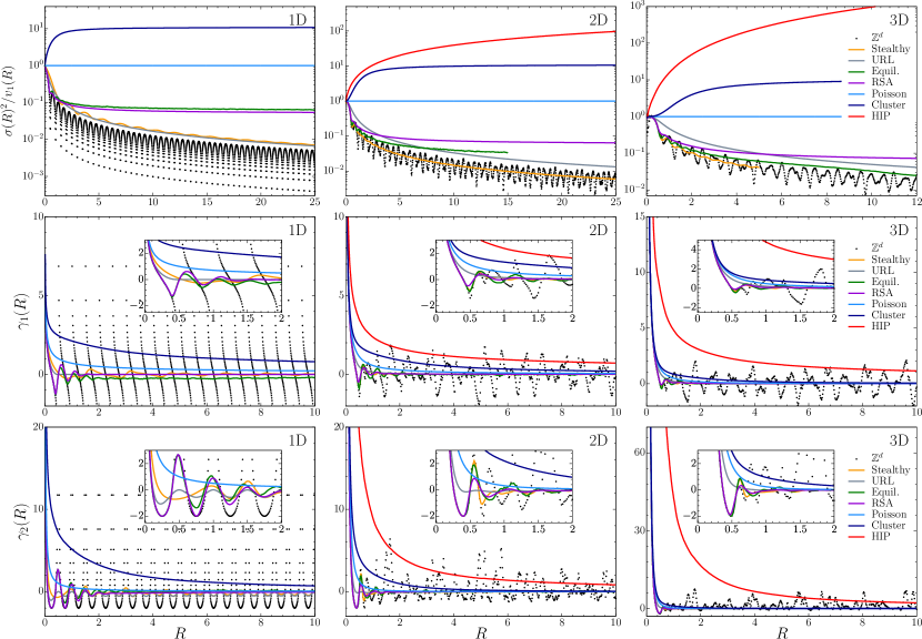
Figure 2: Graphs of the number variance, skewness and excess kurtosis versus the window radius $R$ for all considered models across the first three space dimensions.

For $d\geq 2$, we have found via analyses given in the SM and immediately below that the skewness $\gamma_{1}(R)$ and excess kurtosis $\gamma_{2}(R)$ for our disordered hyperuniform systems vanish faster with increasing $R$ than those for nonhyperuniform systems. Among all models studied, the quantities $\gamma_{1}(R)$ and $\gamma_{2}(R)$ vanish slowest for the antihyperuniform HIP models for $d\geq 2$. The specific decay rates for all models are described below.

It is noteworthy that one-dimensional systems can present fluctuation anomalies not present in higher dimensions. For example, in the case of the integer lattice, the random variable $N(R)$ can only take at most two values for any $R$, which of course is abnormally non-Gaussian. While the hypercubic lattice for $d\geq 2$ never achieves a CLT (as discussed below), the variance is considerably broader than that for $d=1$. Another anomalous category is class I hyperuniform systems, which have bounded variance for $d=1$ [see Eq. (76)] and thus any such hyperuniform point process cannot obey a CLT because the standardized distribution cannot converge to a continuous distribution. This is clearly borne out by the distance metric plots, shown in Fig. 5 and Fig. S8 of the SM, for both the 1D disordered stealthy point process and integer lattice.

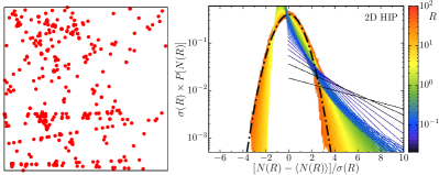
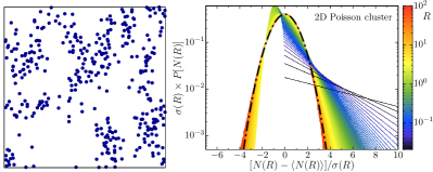
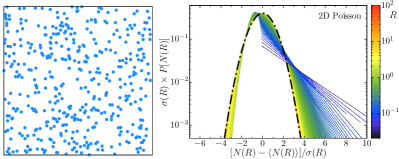
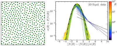
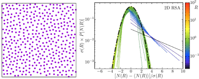
Figure 3: Representative images of configurations of each of the five 2D nonhyperuniform models, beginning with the most nonhyperuniform one (HIP) down to one that has the smallest structure factor at the origin (saturated RSA). The corresponding standardized probability distributions for different window radii are also included; deepest blue color (darkest shade) corresponds to zero radius and the deep orange color corresponds to the largest considered radius.

For the Poisson and super-Poissonian models (cluster and HIP) across dimensions, both the skewness and excess kurtosis decay monotonically; see Fig. 2. By contrast, the skewness and excess kurtosis oscillate about zero for the lattice, stealthy, equilibrium and RSA systems across all dimensions because all of them exhibit at least short-range order. It should not go unnoticed how the oscillations in $\gamma_{1}(R)$ and $\gamma_{2}(R)$ are related to short- or long-range order at the level of three- and four-body correlation functions, $g_{3}$ and $g_{4}$, as can be seen from the explicit formulas (22) and (23) for the skewness and excess kurtosis. In the instances of RSA and equilibrium packings, oscillations in $\gamma_{1}(R)$ and $\gamma_{2}(R)$ arise from strong short-range order exhibited by $g_{3}$ and $g_{4}$.

The disordered hyperuniform systems that we consider, stealthy and URL point processes, have extraordinary number fluctuation behaviors. For 2D and 3D stealthy systems, both $\gamma_{1}(R)$ and $\gamma_{2}(R)$ strongly oscillate about zero; see Fig. 2. This suggests that at the level of $g_{3}$, stealthy systems, counterintuitively, exhibit significant ordering on much larger length scales than the short-range order seen in the pair correlation function Torquato et al. (2015). For 1D stealthy systems, $\gamma_{1}(R)$ and $\gamma_{2}(R)$ show even stronger oscillations than their higher-dimensional counterparts, indeed reflecting possible long-range order present in $g_{3}$ and $g_{4}$. It is remarkable that the skewness and excess kurtosis can detect such anomalous long-range order that would not be expected based solely on the behavior of the pair correlation function. Another reason that supports the capacity of $\gamma_{1}(R)$ and $\gamma_{2}(R)$ to detect unusual long-range order is the cloaked URL model, which at the level of the pair correlation function would be considered to be highly disordered. Whereas $\gamma_{1}(R)$ for this model is a monotonically decreasing function of $R$, $\gamma_{2}(R)$ exhibits oscillations. This is entirely consistent with the fact that the periodicity of the underlying lattice is completely hidden at the level of the three-point correlation function but manifests itself for the first time in $g_{4}$ Klatt et al. (2020).

VII.2 Number Distributions for the Models Across Dimensions

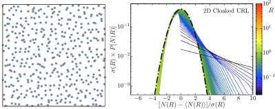
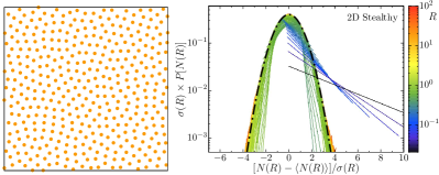
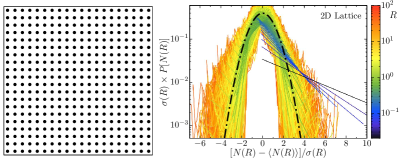
Figure 4: Representative images of configurations of each of the three 2D hyperuniform models and their corresponding standardized probability distributions, where the deepest blue color (darkest shade) corresponds to zero radius and the deep orange color corresponds to the largest considered radius.

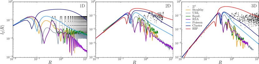
Figure 5: The Gaussian distance metric $l_{2}(R)$ versus the window radius $R$ for all considered models across the first three space dimensions.

Figures 3 and 4 show representative configurations of all of the 2D models and their corresponding standardized number distributions. (We provide corresponding figures for all 1D and 3D models in the SM). Except for hypercubic lattices for any $d$ and 1D hyperuniform systems of class I, all of the considered models across dimensions obey a CLT. It is noteworthy that for all models, except the hypercubic lattices, the number distribution functions $P[N(R)]$ are unimodal, i.e., one with a single peak. (For small radii $R\lessapprox 0.5$, the number distributions are monotonically decreasing, which are still considered to be unimodal.) Recall that for all models, except the hypercubic lattice and the class I hyperuniform models in one dimension, the skewness and excess kurtosis tend to zero for large $R$ for all dimensions. For well-behaved unimodal distributions, such a vanishing of both $\gamma_{1}(R)$ and $\gamma_{2}(R)$ indicates a tendency to a CLT. Indeed, this is confirmed by visual inspection of our corresponding evaluations of the number distributions for all dimensions; see Figs. 3 and 4. Our conclusions about the tendencies to CLTs for sufficiently large $R$ are further confirmed by our evaluations of the Gaussian distance metric $l_{2}(R)$ for all models across dimensions, which are plotted in Fig. 5. For $d=2$ and $d=3$, one clearly sees that disordered hyperuniform point processes are better approximated by the normal distribution than their nonhyperuniform counterparts at a given large value of $R$. This is consistent with the visual inspections of the plots presented Figs.  3 and 4. From Fig. 5 and Fig. S8 of the SM, one can ascertain, for each model, a radius $R_{0}$ above which the distribution can be deemed to be approximately Gaussian, i.e., $l_{2}(R)$ is below some threshold for $R>R_{0}$, implying that it is approximately determined by only the mean and the variance. Typically, we find that $R_{0}$ is orders of magnitude smaller for our hyperuniform and standard nonhyperuniform models than for our super-Poissonian models.

Our results clearly show that the hypercubic lattices across dimensions do not obey a CLT; see Figs. 2, 4 and 5. This is due to the fact that lattice points in general are “rigid” in the sense that fluctuations in $N(R)$ are always stringently bounded from below and above for any value of $R$ (as discussed in Sec. III.3) due to their inherent long-range order. Hence, $P[N(R)]$ is highly sensitive to the value of $R$, so that both $\gamma_{1}(R)$ and $\gamma_{2}(R)$ rapidly oscillate around zero, but the amplitudes of the oscillations do not vanish as $R$ increases. It is already well-established that the local variance $\sigma^{2}(R)$ of lattices exhibits such rapid oscillations; see Ref. Torquato and Stillinger (2003) and references therein. Because of the rapid oscillations in $\gamma_{1}(R)$, $\gamma_{2}(R)$, and $l_{2}(R)$ for hypercubic lattices, we represent the data by points instead of curves, which would require interpolation between the data points. Note that the corresponding distance metrics $l_{2}(R)$ are bounded from below for any value of $R$. These observations are consistent with the visual inspections of the number distribution shown in Fig. 4 for $d=2$ and those for $d=1$ and $d=3$ given in the SM.

VII.3 Gamma-Distribution Approximation for All Models Obeying a CLT

Table 2: Large-$R$ asymptotic scalings of $\sigma^{2}(R)$, $\gamma_{1}(R)$, $\gamma_{2}(R)$ and $l_{2}(R)$ for all of our models across dimensions that obey a CLT, as obtained by the approximation of $P[N(R)]$ by the gamma distribution function for each model for any $d$.

Descriptor	Stealthy & URL	Cluster, Poisson, RSA, & Equilibrium	HIP
$\sigma^{2}(R)$	$R^{(d-1)}$	$R^{d}$	$R^{2d-1}$
$\gamma_{1}(R)$	$R^{-(d+1)/2}$	$R^{-d/2}$	$R^{-1/2}$
$\gamma_{2}(R)$	$R^{-(d+1)}$	$R^{-d}$	$R^{-1}$
$l_{2}(R)$	$R^{-(d+1)/2}$	$R^{-d/2}$	$R^{-1/2}$

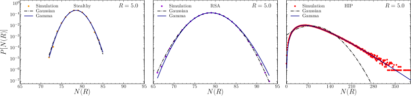
Figure 6: Comparison of simulation data for the probability distributions $P[N(R)]$ with $R=5$ for three 2D models (stealthy hyperuniform, RSA, and HIP) to corresponding gamma-distribution approximations with the same mean value and variance. The gamma distribution provides good approximations for all models that obey a CLT across the first three dimensions considered, including the ones not shown here.

We have studied a variety of well-known closed-form probability distributions to determine those which best approximate the actual distributions for finite $R$ for all of our models. Remarkably, we have ascertained that the gamma distribution provides a good approximation to the number distribution $P[N(R)]$ for all models that obey a CLT across all dimensions for intermediate to large values of $R$. (Recall that the hypercubic lattices and 1D hyperuniform systems do not obey a CLT.) The gamma distribution is defined by

$$P[N(R)=m]=\frac{1}{\Gamma(k)\theta^{k}}m^{k-1}e^{-m/\theta},$$ (84)

where $k$ and $\theta$ are shape and scale parameters, respectively, which are related to the mean and variance of $P[N(R)]$ as follows:

$$\langle N(R)\rangle= k\theta,$$ (85)

$$\sigma^{2}(R)= k\theta^{2}.$$ (86)

It immediately follows that the associated skewness and excess kurtosis can be expressed simply in terms of the mean and number variance, yielding

$$\gamma_{1}(R)= \frac{2}{\sqrt{k}}=2\quantity[\frac{\sigma^{2}(R)}{{\langle N(R)\rangle}^{2}}]^{1/2},$$ (87)

$$\gamma_{2}(R)= \frac{6}{k}=6\quantity[\frac{\sigma^{2}(R)}{{\langle N(R)\rangle}^{2}}].$$ (88)

Figure  6 compares the gammma-distribution approximations to simulation data for a representative disordered hyperuniform model (stealthy), a standard nonhyperuniform model (RSA) and an antihyperuniform model (HIP) in two dimensions for $R=5$. Visual inspection reveals the gamma distribution provides a good approximation in each case. Similar good agreement between the gamma-distribution approximation and simulation data was found for other models (not shown in Fig. 6) obeying a CLT across dimensions, as discussed in the SM.

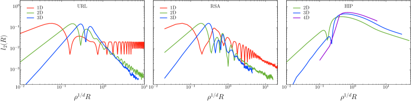
Figure 7: The Gaussian distance metric $l_{2}(R)$ versus $R$ for a representative disordered hyperuniform model (URL), sub-Poisson nonhyperuniform model (RSA) and anti-hyperuniform model (HIP) across the first three space dimensions, respectively.

Importantly, the approximation of $P[N(R)]$ by a gamma distribution enables us to estimate the large-$R$ scalings of $\gamma_{1}(R)$ and $\gamma_{2}(R)$ for all models across dimensions that obey a CLT. Specifically, we find $\gamma_{1}(R)\sim R^{-1/2}\text{~{}and~{}}\gamma_{2}(R)\sim R^{-1}$ for the antihyperuniform HIP, $\gamma_{1}(R)\sim R^{-d/2}\text{~{}and~{}}\gamma_{2}(R)\sim R^{-d}$ for standard nonhyperuniform models, and $\gamma_{1}(R)\sim R^{-(d+1)/2}\text{~{}and~{}}\gamma_{2}(R)\sim R^{-(d+1)}$ for the hyperuniform models. Table 2 summarizes these scaling behaviors. The fact that the excess kurtosis decays to zero faster than the skewness for any model that obeys a CLT, whether hyperuniform or not, implies that the dominant asymptotic correction of the gamma distribution to a CLT for large $R$ is determined by the skewness; see Appendix A for a proof. It is noteworthy that these predictions based on the gamma distribution are consistent with numerical findings for all nonhyperuniform systems and the antihyperuniform HIP using an independent method that employs certain running averages of $\gamma_{1}(R)$ and $\gamma_{2}(R)$; see the SM for details. Moreover, for 2D and 3D disordered hyperuniform (stealthy and URL) models, the predictions from the gamma-distribution approximations are also consistent with the observed scalings of the skewness. Due to the strong oscillations in the excess kurtosis for 2D and 3D stealthy and URL processes described above, it was numerically difficult to definitively determine their scalings from the running-average method. It should not go unnoticed that the exact formulas for the skewness and excess kurtosis, Eqs. (34) and (35), respectively, of the Poisson distribution are consistent with the scalings predicted by the gamma-distribution approximation, lending additional validity to the latter. Furthermore, we have found that for all models across dimensions that obey a CLT, the running-average procedure yields scalings for $l_{2}(R)$ that agree with the corresponding gamma-distribution approximations (see SM), which are identical to the scalings for the skewness $\gamma_{1}(R)$. The proof that $l_{2}(R)$ has exactly the same scaling as $\gamma_{1}(R)$ for the gamma distribution is given in Appendix A. Furthermore, our approximations of $P[N(R)]$ by gamma distributions are also consistent with CLTs, since they converge to the Gaussian distribution in the limit of $k\to\infty$ (i.e, $R\to\infty$), as described in Appendix A.

According to Table 2, convergence to a CLT is slowest for the HIP (proportional to $R^{-1/2}$ for $d\geq 2$), followed by the Poisson cluster process, and the Poisson process. RSA and equilibrium packings have the same scaling behaviors as the Poisson cluster and Poisson processes, but with smaller coefficients of proportionality. The convergence to a CLT is fastest for the disordered hyperuniform processes for $d=2$ and $d=3$ 

VII.4 Effect of Dimensionality on the Approach to a CLT

For any particular $d$-dimensional model that eventually obeys a CLT, does the number distribution function $P[N(R)]$ tend to Gaussian-like behavior faster as the space dimension $d$ increases? As noted in the Introduction, this question can be answered by appealing to the decorrelation principle Torquato and Stillinger (2006a), which states unconstrained correlations in disordered packings that exist in low dimensions vanish as $d$ tends to infinity, and all higher-order correlation functions $g_{n}$ for $n\geq 3$ may be expressed in terms of the number density $\rho$ and pair correlation function $g_{2}$. The decorrelation principle begins to manifest itself in low dimensions for disordered packings Skoge et al. (2006); Torquato and Stillinger (2006b); Torquato et al. (2006) but other disordered systems with strongly repulsively interacting particles, including fermionic Torquato et al. (2008) and Gaussian-core point processes Zachary et al. (2008). We know that the number distribution function $P[N(R)]$ generally involves certain integrals over all of the $n$-body correlation functions. Therefore, the decorrelation principle implies that for any $d$-dimensional model that decorrelates with $d$, $P[N(R)]$ increasingly becomes Gaussian-like as $d$ increases, since the first and second moments, determined by $\rho$ and $g_{2}$, dominate the distribution. By the same token, for any model that correlates with increasing $d$, $P[N(R)]$ increasingly deviates from the normal distribution as $d$ increases. We have verified these broad conclusions for the models studied in this article. In Fig. 7, we plot the Gaussian distance metric $l_{2}(R)$ for a representative disordered hyperuniform model (URL), a sub-Poisson nonhyperuniform model (RSA) and an anti-hyperuniform model (HIP) across the first three space dimensions, respectively. (Recall that the URL obeys a CLT for $d\geq 2$.) As expected, we see that for both the URL and RSA models for a fixed value of $R$ (for $R>1$), $l_{2}(R)$ decreases with increasing $d$ (increasingly tends to Gaussian-like behavior) because of decorrelation, while for the HIP, $l_{2}(R)$ increases with increasing $d$ (moves away from Gaussian-like behavior) because it increasingly correlates with $d$. Importantly, when comparing fluctuations across dimensions, one must choose a meaningful length scale to make the window radius $R$ dimensionless. A simple and good choice is $\rho^{1/d}$, which is proportional to the mean nearest-neighbor distance in space dimension $d$, and explains why the horizontal axes in each subfigure of Fig. 7 is $\rho^{1/d}R$.

VIII Conclusions and Discussion

Via theoretical methods and high-precise simulation studies, we accurately quantified the skewness $\gamma_{1}(R)$, excess kurtosis $\gamma_{2}(R)$ and the number distribution $P[N(R)]$ for eight different models of statistically homogeneous point processes in two and three dimensions: five nonhyperuniform models, one of which is anti-hyperuniform (HIP), and three hyperuniform models. Analogous models were also examined in one dimension, except for HIP, which is not defined in this dimension. We validated our simulation results for $\gamma_{1}(R)$, $\gamma_{2}(R)$ and $P[N(R)]$ for all models by showing that they are in excellent agreement with rigorous bounds and exact results that we derived for the applicable ranges of $R$. For all disordered hyperuniform models, our explicit general formulas for $\gamma_{1}(R)$ and $\gamma_{2}(R)$ in terms of $n$-body information [Eqs. (22) and (23)] enable us to infer the existence of “hidden” type of long-range order that manifests itself for the first time at the three-body level or higher. Thus, the skewness and excess kurtosis have the capacity to detect anomalous long-range order that would not be expected based on the behavior of the pair correlation function alone.

We have introduced a novel Gaussian “distance” metric $l_{2}(R)$ to ascertain the proximity of $P[N(R)]$ to the normal distribution for each model as a function of $R$. We have verified that $l_{2}(R)$ is a sensitive metric via numerical and theoretical methods. Since the distributions for all models (except the lattices) across dimensions are unimodal, the tendency to a CLT corresponds to the skewness and excess kurtosis simultaneously tending to zero. Almost all of the considered models across dimensions obey a CLT. We found that disordered hyperuniform point processes are better approximated by the normal distribution than their nonhyperuniform counterparts at a given large value of $R$. We proved that any 1D hyperuniform system of class I as well as the hypercubic lattice for any $d$ cannot obey a CLT. Similarly, a general lattice in any dimension cannot obey a CLT.

It is noteworthy that we discovered that the gamma distribution provides a good approximation to the number distribution $P[N(R)]$ for all models that obey a CLT across all dimensions for intermediate to large values of $R$, enabling us to estimate the large-$R$ scalings of $\gamma_{1}(R)$, $\gamma_{2}(R)$ and $l_{2}(R)$. These predictions were corroborated by corresponding simulation results in almost all instances, as detailed in the SM. It is only in the special cases of the excess kurtosis for 2D and 3D stealthy and URL processes where the running-average method was not reliable enough to definitively determine their scalings due to strong oscillations, and thus this represents a simulation challenge for future research. Among all models, the convergence to a CLT is generally fastest for the disordered hyperuniform processes in two and three dimensions such that $\gamma_{1}(R)\sim l_{2}(R)\sim R^{-(d+1)/2}$ and $\gamma_{2}(R)\sim R^{-(d+1)}$ for large $R$. The convergence to a CLT is slower for standard nonhyperuniform models such that $\gamma_{1}(R)\sim l_{2}(R)\sim R^{-d/2}\text{~{}and~{}}\gamma_{2}(R)\sim R^{-d}$. Not surprisingly, the convergence to a CLT is slowest for the antihyperuniform HIP model such that $\gamma_{1}(R)\sim l_{2}(R)\sim R^{-1/2}\text{~{}and~{}}\gamma_{2}(R)\sim R^{-1}$. Using the decorrelation principle, we elucidated why any $d$-dimensional model that “decorrelates” or “correlates” with $d$ corresponds to a $P[N(R)]$ that increasingly moves toward or away from a CLT, respectively.

It has recently been reported that in a 2D absorbing phase of a lattice gas model, the density distribution at a hyperuniform length scale increasingly deviates from a Gaussian distribution on approach to the critical point Zheng and Ciamarra (2020), corresponding to a class III hyperuniform system Torquato (2018a). These distributions are distinguished from those of our models in that they have heavy left tails ($\gamma_{1}(R)<0$). This implies that they cannot be approximated by gamma distributions, as in the majority of the models studied in the present paper across dimensions.

A related but distinctly different study from the one considered in the present work concerns fluctuations when the window is centered on a point of the point process Torquato et al. (1990); Truskett et al. (1998). It will be interesting in future work to carry out the analogous investigation of the corresponding skewness, excess kurtosis and number distribution for such particle-based quantities for hyperuniform and nonhyperuniform models.

Appendix A Asymptotic Behavior of $l_{2}(R)$ for the Gamma Distribution

We prove that the large-$R$ scalings of the distance metric $l_{2}(R)$ and the skewness $\gamma_{1}(R)$ are the same for the gamma distribution. It is important to note that the asymptotic analysis is facilitated by transforming the random variable $N(R)$ to the standardized random variable $X\equiv(N(R)-\langle N(R)\rangle)/\sigma(R)$. In the large-$R$ limit, the discrete random variable tends to a continuous one and hence the continuous-variable analog of the distance metric $l_{2}(R)$, defined Eq. (81), is given by

$$l_{2}(R)\equiv\left[\int_{-\infty}^{\infty}|F_{G}(X)-F_{\Gamma}(X)|^{2}dX\right]^{1/2}$$ (89)

where $F_{G}(X)$ and $F_{\Gamma}(X)$ are the cumulative distribution functions for the Gaussian and gamma distribution functions, respectively. Specifically,

$$F_{G}(X)=\frac{1}{2}\left[1+\mbox{erf}(X/\sqrt{2})\right]$$ (90)

and

$$F_{\Gamma}(X)=1-\frac{\Gamma(k,X\sqrt{k}+k)}{\Gamma(k)}$$ (91)

where $\Gamma(s,y)=\int_{y}^{\infty}t^{s-1}\exp(-t)dt$ is the upper incomplete gamma function.

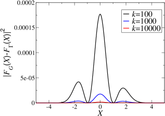
Figure 8: Integrand of (89) versus $X$ for select values of the shape parameter $k$.

Since the $(n+1)$th cumulant of the gamma distribution tends to zero faster than its $n$th cumulant for $n\geq 3$, the greatest deviation of the gamma distribution from the normal one occurs in the vicinity of the origin, i.e., $X=0$, in the large $k$-limit (see Fig. 8) and is thus dominated by the asymptotic behavior of the skewness. Thus, we require the Taylor series expansions of the distributions about $X=0$:

$$F_{G}(X)= \frac{1}{2}+\frac{1}{2}\sqrt{\frac{2}{\pi}}X-\frac{1}{12}\sqrt{\frac{2}{\pi}}X^{3}+\frac{1}{80}\sqrt{\frac{2}{\pi}}X^{5}$$

$$-\frac{1}{672}\sqrt{\frac{2}{\pi}}X^{7}+{\cal O}(X^{9})$$ (92)

$$F_{\Gamma}(X)= a_{0}(k)+a_{1}(k)X+a_{2}(k)X^{2}+a_{3}(k)X^{3}$$

$$+a_{4}(k)X^{4}+a_{5}(k)X^{5}+a_{6}(k)X^{6}+a_{7}(k)X^{7}$$

$$+a_{8}(k)X^{8}+{\cal O}(X^{9}),$$ (93)

where the coefficients $a_{m}(k)$ ($m=1,2,3,\ldots)$ depend on the shape parameter $k$. We know these coefficients explicitly but do not indicate them for reasons of brevity. The corresponding large-$k$ asymptotic expansions of the first nine coefficients are

$$a_{0}(k) = \frac{1}{2}+\frac{1}{6}\sqrt{\frac{2}{k\pi}}+{\cal O}(1/k)$$ (94)

$$a_{1}(k) = \frac{1}{2}\sqrt{\frac{2}{\pi}}+{\cal O}(1/k)$$ (95)

$$a_{2}(k) = -\frac{1}{4}\sqrt{\frac{2}{k\pi}}+{\cal O}(1/k^{3/2})$$ (96)

$$a_{3}(k) = -\frac{1}{12}\sqrt{\frac{2}{\pi}}+{\cal O}(1/k)$$ (97)

$$a_{4}(k) = \frac{5}{48}\sqrt{\frac{2}{k\pi}}+{\cal O}(1/k^{3/2})$$ (98)

$$a_{5}(k) = \frac{1}{80}\sqrt{\frac{2}{\pi}}+{\cal O}(1/k)$$ (99)

$$a_{6}(k) = -\frac{7}{288}\sqrt{\frac{2}{k\pi}}+{\cal O}(1/k^{3/2})$$ (100)

$$a_{7}(k) = -\frac{1}{672}\sqrt{\frac{2}{\pi}}+{\cal O}(1/k)$$ (101)

$$a_{8}(k) = \frac{1}{256}\sqrt{\frac{2}{k\pi}}+{\cal O}(1/k^{3/2})$$ (102)

We see that for odd $m$, the leading-order terms of $a_{m}$ are exactly the same as the coefficients multiplying $X^{m}$ in the series expansion (92) for the standard normal distribution. Thus, combining (92), (93) and the aforementioned asymptotic expansions yield

$$F_{\Gamma}(X)-F_{G}(X)=\frac{f(X)}{\sqrt{k}}+{\cal O}(\frac{1}{k^{3/2}}),$$ (103)

where $f(X)$ is a function that is localized about the origin with the following corresponding Taylor series expansion:

$$f(X)=\sqrt{\frac{2}{\pi}}\left[\frac{1}{6}-\frac{1}{4}X^{2}-\frac{5}{48}X^{4}-\frac{7}{288}X^{6}-\frac{1}{256}X^{8}+{\cal O}(X^{10})\right].$$ (104)

Substitution of (103) into (89) gives the large-$k$ asymptotic expansion of the Gaussian distance metric, i.e.,

$$l_{2}(R)=\frac{c}{\sqrt{k}}+{\cal O}(\frac{1}{k^{3/2}}),$$ (105)

where the square of the constant $c$ is given by

$$c^{2}=\int_{-\infty}^{\infty}f^{2}(X)dX.$$ (106)

Finally, since the skewness $\gamma_{1}(R)$ scales like $1/\sqrt{k}$, we conclude that $l_{2}(R)\sim\gamma_{1}(R)$ for large values of $R$. Note that the vanishing of $l_{2}(R)$ for $R\to\infty$ implies a CLT for the gamma distribution as described in the text.