Algorithms for Contractibility of Compressed Curves on 3-Manifold Boundaries
Abstract
In this paper we prove that the problem of deciding contractibility of an arbitrary closed curve on the boundary of a 3-manifold is in NP. We emphasize that the manifold and the curve are both inputs to the problem. Moreover, our algorithm also works if the curve is given as a compressed word. Previously, such an algorithm was known for simple (non-compressed) curves, and, in very limited cases, for curves with self-intersections. Furthermore, our algorithm is fixed-parameter tractable in the complexity of the input 3-manifold.
As part of our proof, we obtain new polynomial-time algorithms for compressed curves on surfaces, which we believe are of independent interest. We provide a polynomial-time algorithm which, given an orientable surface and a compressed loop on the surface, computes a canonical form for the loop as a compressed word. In particular, contractibility of compressed curves on surfaces can be decided in polynomial time; prior published work considered only constant genus surfaces. More generally, we solve the following normal subgroup membership problem in polynomial time: given an arbitrary orientable surface, a compressed closed curve , and a collection of disjoint normal curves , there is a polynomial-time algorithm to decide if lies in the normal subgroup generated by components of in the fundamental group of the surface after attaching the curves to a basepoint.
1 Introduction
In a topological space , a closed curve is contractible if the map extends to a map of the standard disk, , ; such a curve can be continuously deformed to a point, and represents the trivial homotopy class for the fundamental group of the space. Dating back to Dehn [12] more than a century ago, the problem of testing contractibility has been an important focus in the development of efficient algorithms in computational topology and group theory. Such problems are now well understood in two dimensions, with recent works of the second author and Rivaud [30] and Erickson and Whittlesey [17] providing linear-time algorithms to test contractibility and free homotopy of curves on surfaces; Despré and the second author [13] also developed efficient algorithms for the closely related problem of computing the geometric intersection number of curves. On the other hand, in higher dimensions, homotopy problems quickly become undecidable: testing contractibility of curves is already undecidable on -dimensional simplicial complexes and in -manifolds (see Stillwell [41, Chapter 8]).
The aim of this paper is to further improve our understanding of the intermediate -dimensional case. In a -manifold, testing whether a curve is contractible is known to be decidable, but the best known algorithms are intricate and rely on the proof of the Geometrization Conjecture. We refer to the survey of Aschenbrenner, Friedl and Wilton [2]. When the input manifold is a knot complement, this problem contains as a special case the famous Unknot Recognition problem, which asks whether an input knot in is trivial. That problem is now known to be in NP [19] and co-NP [27]. Recently, Colin de Verdière and the fourth author [10] initiated the study of a problem in between those two, which is testing the contractibility of a closed curve which lies on the boundary of a triangulated -manifold , and they provided an algorithm to solve this problem in time . They asked whether the problem lies in the complexity class NP and proved that it holds in two cases: when the number of self-intersections of is at most logarithmic, and when the boundary surface is a torus. We remark that the existence of an algorithm to test contractibility of a closed curve on the boundary actually follows from the earlier results of Waldhausen [42], and an exponential-time algorithm can be derived from the standard 3-manifold literature, as we will explain later in this paper. However, the algorithm of [10, 11] is simpler in the sense that it relies only on the proof of the Loop Theorem.
Our main result is that the problem of contractibility when the curve is on the boundary of the 3-manifold is in NP. Furthermore, the algorithm that we provide has two additional features. First, it is fixed parameter tractable in the input manifold: for a given -manifold , after a preprocessing taking exponential time in , we can solve any contractibility test for curves on the boundary in polynomial time. Second, our algorithm also works if the input curve is compressed via a straight-line program, in particular, it can be exponentially longer than its encoding size (we defer to Section 2 for the precise definitions).
Theorem 1.
Let a triangulated -manifold and a curve on the boundary of be given as the input. The problem of deciding whether is contractible in is in NP, and there is a deterministic algorithm that solves the problem in time . This is also the case if is given as a compressed word, i.e., a straight-line program.
Our proof of Theorem 1 will reduce the problem to another problem involving only curves on surfaces. However, there is an important subtlety. Many algorithms in -dimensional topology involve an exponential blow-up in the size of the objects under consideration. This is the case for example for Unknot Recognition, where the classical algorithm [19] looks for a disk spanning the knot, but this disk might be exponentially large [20]. In order to get NP membership, this exponential blow-up is controlled using a compressed111There are two different forms of compression going on in this paper: normal coordinates and straight line programs. We keep the name compressed for the latter, while a curve or a multicurve encoded with normal coordinates will be simply called a normal (multi-)curve. system of coordinates called normal coordinates (see Section 2 for definitions). Our approach follows a similar scheme and suffers from a similar blow-up, which forces us to deal with normal curves. Precisely, we show that the problem of contractibility of an arbitrary curve on the boundary of a 3-manifold reduces to the following problem. Given a family of disjoint normal closed curves on a triangulated surface , and a curve on , decide if lies in the normal subgroup of the fundamental group determined by the curves of (appropriately connected to the basepoint). This is equivalent to deciding if the curve is contractible in the space resulting from by gluing a disk to each component of . We call this problem the disjoint normal subgroup membership problem, and we provide an algorithm to solve it in polynomial time, despite the highly compressed nature of and .
Theorem 2.
Let an orientable triangulated surface , a closed normal multi-curve , and a compressed curve be given as the input. There is a polynomial-time algorithm for deciding the disjoint normal subgroup membership problem for and on .
To solve the disjoint normal subgroup membership problem, one of our technical tools is a polynomial-time algorithm to test triviality of a compressed closed curve on a surface, which might be of independent interest. In fact, we compute a canonical form for such a curve, in the sense that there is a unique canonical representative in each based homotopy class.
Theorem 3.
Let an orientable triangulated surface and a compressed loop on described by a straight-line program be given. Then one can transform , in polynomial time, into a canonical form in its based homotopy class, given as a compressed word. In particular, we can test in polynomial time whether is contractible.
We emphasize that in Theorem 3 the surface is part of the input. The analogous theorem, if we assume that surface is not part of the input, has been known in a much broader context, as we discuss in the next section.
1.1 Related work
Algorithms in -manifold topology
There is now a large body of research on the computational complexity of problems in -manifold topology and knot theory. To paint a picture in broad strokes, most topological problems are now known to be decidable, using a combination of geometric, algebraic and topological tools and the complexity of the best known algorithms range from exponential [19, 1] to quite galactic, see for example Kuperberg [26] for the homeomorphism problem. In contrast, only very few complexity lower bounds are known [1, 28, 9] and for many problems, including ours, it is open whether a polynomial-time algorithm exists. One particular tool that our work relies on is normal surface theory, which provides a powerful framework to enumerate and analyze the topologically relevant embedded surfaces in a -manifold. Actually, tools from normal surface theory [40] provide an off-the-shelf algorithm proving that deciding contractibility of a simple curve on the boundary of a -manifold is in NP, as explained in [10, Section 3]. However, normal surface theory is ill-adapted to study surfaces that are not embedded [5], hence the more technical path that we follow in this paper. We refer to Lackenby [29] for a recent and extensive survey on algorithms in -manifold topology.
Geometric and combinatorial group theory
The problem of deciding the contractibility of a curve in a topological space, which is given for example as a finite simplicial complex, can be equivalently rephrased as a problem of testing the triviality of a word in a finitely presented group, the fundamental group of the space. In the case of 2- and 3-manifolds, the geometry or topology of the underlying manifold has a strong impact on the properties of the group, and there is a vast amount of literature on this interaction, see for example [8]. We refer to Aschenbrenner, Friedl and Wilton [2, 3] for the case of -manifold groups. Of particular interest for the word problem is the notion of a Dehn function, which upper bounds the area of a disk certifying the triviality of a word, and thus controls the complexity of a brute-force algorithm to solve the word problem. For -manifold groups, this function can be exponential [7, Theorem 8.1.3], making such an approach at least exponentially worse than ours. When the Dehn function of a group presentation is polynomial (as is the case, for instance, for the fundamental group of a compression body), it can be used to prove that the word problem is in NP. However, this only works for a fixed presentation. In our problem, the group presentation itself is part of the input, and we cannot use the bound on the Dehn function directly.
Algorithms for compressed curves and surfaces
As we hinted at in the introduction, -dimensional algorithms naturally tend to involve exponentially large objects, which are generally compressed using normal coordinates. This incurs a need for efficient algorithms dealing with normal curves and surfaces, even for the most basic tasks. For example, it is not easy to test whether a curve described by normal coordinates is connected. By now, there are many known techniques to handle topological problems on compressed curves, see for example Agol, Hass and Thurston [1], Schaefer, Sedgwick and Stefankovič [37, 38], Erickson and Nayyeri [16], Bell [4] or Dynnikov [14] and Dynnikov and Wiest [15]. None of these techniques seem to directly solve our disjoint normal subgroup membership problem, but we rely extensively on the work of Erickson and Nayyeri [16] as a subroutine (see Section 4). However, normal coordinates do not describe curves with self-intersections, which are our main object of interest in this paper. This is why we rely on a different compression model in the form of straight-line programs. The use of such programs in geometric group theory is not new, and in particular there is a sketch of an algorithm to test triviality of compressed curves on a surface of genus in an appendix of Schleimer [39, Appendix A]. His approach seems to be readily generalizable to higher genus, but the dependency on the genus is not made explicit. More recently, Holt, Lohrey and Schleimer [23] provided a polynomial-time algorithm to test triviality of compressed words in hyperbolic groups, of which (most) surface groups are a subclass. The difference with our Theorem 3 is that in their result, the group presentation is not part of the input. While both approaches could plausibly be used in our setting, we rely on different tools to provide a complete proof of Theorem 3: our approach treats the surface as an input and works for any genus, and seamlessly generalizes to the case of wedges of surfaces that we also need.
1.2 Summary of our techniques
The standard methods of normal surface theory allow us to reduce our main contractibility problem to the case where the input manifold belongs to a particular class of manifolds called compression bodies, see Section 3. The fundamental group of compression bodies is roughly a free product of surface groups, and thus one can rely on known algorithms for surfaces [17, 30] to solve the contractibility problem there. However, due to the exponential size of normal surfaces, this would only yield an exponential time algorithm. In order to improve on this, we identify the precise problem that we need to solve to be the disjoint normal subgroup membership problem and set out on a quest to solve it efficiently. While an NP algorithm would suffice for our main result, we will develop a polynomial-time algorithm.
The disjoint normal subgroup membership problem is made delicate by the compressed nature of the curves in . If they were given as disjoint curves, say, on the -skeleton of the surface, we could glue a disk on each of them, and observe that the resulting complex is homotopically equivalent to a wedge of surfaces222A wedge of a family topological spaces is the space obtained after attaching them all to a single common point. Actually, there are also circle summands here – we do not mention them in this outline to keep the discussion light., allowing us to reduce the problem to the triviality of a curve in a surface (see Section 5 for a description of the homotopy equivalence). In order to do so despite the compression, we compute in Section 4 a retriangulation of the surface, so that the curves in are only polynomially long in the new triangulation. This is done by tracing the normal curve and building the street complex which was specifically designed by Erickson and Nayyeri to handle normal curves on surfaces in polynomial time. We then track how the street complex interacts with our input curve . This operation comes at a cost: even if the input curve was not compressed, it may become exponentially long after the retriangulation. Since it may be not simple, we rely on straight-line programs instead of normal curves to encode it. At this stage, we note that it might as well have been a compressed straight-line program from the start.
Finally, we want to test the triviality of a compressed curve in a wedge of surfaces. The fundamental group of this wedge is a free product of fundamental groups of surfaces, and thus the crux of the problem is to solve it in a single surface. While there are known techniques to test the contractibility of a curve on a surface, based on local simplification rules [17, 30], the compressed nature of our curves is once again a stumbling block here, as we need to be careful to never apply an exponential number of such simplification rules. The solution sketched by Schleimer [39, Appendix A] to that issue is to introduce a family of well-tempered paths, which are carefully designed to not necessitate such exponential simplifications. We use a different approach: we rely on the standard tools developed for the non-compressed case, namely quad systems and turn sequences, and detect exponential simplification and realize them all at once in polynomial time. This relies on recent insights on the structure of these quad systems [13] [31, Section 4.3].
2 Background
We begin by recalling some key definitions and results, although we assume that the reader is familiar with basic algebraic topology such as homotopy and fundamental groups; we refer to Hatcher [21] or Stillwell [41] for more detailed definitions.
2.1 3-dimensional Manifolds
A -manifold is a topological space where each point is locally homeomorphic to a -dimensional ball or a -dimensional half-ball. The points of the latter type form the boundary of the -manifold, which is always a surface. In this paper, -manifolds are always assumed to be triangulated, and we use common and a less restrictive definition than simplicial complexes: a triangulation of a -manifold is a collection of abstract tetrahedra, along with a collection of gluing pairs which identify some of the boundary triangles in pairs. In particular, we allow two faces of the same tetrahedron to be identified. If we add the further restriction that the neighborhood of each vertex is a -ball or a half -ball and no edge gets glued to itself with the opposite orientation, then the resulting space is always a 3-manifold [36].
We briefly recall normal surface theory, which will be used in Section 3, and refer the reader to Hass, Lagarias and Pippenger [19] and Burton [6] for a more detailed overview and background of the topic. A normal isotopy is an isotopy of a triangulated -manifold that leaves each cell of the triangulation invariant. A normal surface in a triangulation is a properly embedded surface transverse to the triangulation; such a surface decomposes into a disjoint collection of normal disks, each embedded in a single tetrahedron. Each disk inside a tetrahedra is either a triangle, which separates one vertex in a tetrahedron from the others, or a quadrilateral which separates two vertices from the other two. In each tetrahedron, there are (up to normal isotopy) four types of such triangles, and three types of quadrilaterals. The normal surface can be reconstructed using only the number of these triangles and quadrilaterals in each tetrahedron, as long the collection of disks satisfies a family of equations called matching equations and has at most one quadrilateral type in each tetrahedron. These numbers are called the normal coordinates, and since bits encode numbers up to , these normal coordinates naturally have exponential compression: normal coordinates of polynomial bit-size encode surfaces containing possibly exponentially many normal disks. Nevertheless, one can compute the Euler characteristic of a normal surface in polynomial time in the bit-size encoding, since it is a linear form [19, Formula 22]. Finally, crushing a triangulation along a normal surface roughly consists, for each tetrahedron containing at least one quadrilateral, in removing that quadrilateral and gluing its neighbours pairwise along the two pair of edges not intersected by the quadrilateral, as in Figure 1. Then one tears apart in multiple components the triangulation at the places where it is not a -manifold. This can be done in polynomial time, and surprisingly, this very destructive process has a well-controlled topological meaning when the normal surface is a sphere [6].
2.2 Curve and surface representations
We shall often represent a surface by a graph cellularly embedded in that surface. This embedding is encoded as a combinatorial surface thanks to a rotation system over the edges of the graph [35]. Equivalently, one can define a combinatorial surface as a gluing of polygons whose sides are pairwise identified. When all the polygons are triangles, we speak of a triangulation, or a triangulated surface. Note that we allow a triangle to have two sides identified after the gluing or two triangles to share two vertices but no edge, etc.
The complexity of a surface is the number of cells (vertices, edges and faces) of the complex induced by the graph embedding. A curve on such a surface can be represented or encoded in a variety of ways. For instance, any curve is homotopic to a curve defined by a walk on the 1-skeleton of the complex. The complexity of the curve is the number of edges in the walk counted with repetition. One can also consider curves in general position avoiding the vertices of the graph and cutting its edges transversely as in the next section, in which case we say the complexity of a curve is its number of intersection points with the graph.
We next outline two different notions of compressed curve representations. To repeat the footnote of warning in the introduction: normal coordinates and straight line programs are two different methods for compressed representations, both of which we use in this paper. We keep the name compressed for straight line programs, while a curve or a multicurve encoded with normal coordinates will be simply called a normal (multi-)curve.
Normal curves
Let be a triangulated surface. A multi-curve is a disjoint family of curves embedded on a . A multi-curve is normal if it is in general position with respect to the triangulation of and if every maximal arc of in a triangle has its endpoints on distinct sides. In particular, no component of a normal curve is contained in a single triangle. A normal curve may have three types of arcs in a triangle, one for each pair of sides. Counting the number of arcs of of each type in each of the triangles of the triangulation, we get numbers called the normal coordinates of . As for triangulated 3-manifolds, a normal isotopy of is an isotopy that leaves each cell of the triangulation invariant. Up to a normal isotopy, is completely determined by its normal coordinates. It is thus possible to encode a multi-curve with exponentially many arcs by storing its normal coordinates, which then have polynomial bit-complexity. A normal multi-curve is reduced if no two of its components are normally isotopic.
Straight-line programs
Another method of compressing curves is to think of a curve as a word over an alphabet. In this encoding, a letter of the alphabet corresponds to a directed edge on the surface and juxtaposition of letters corresponds to concatenation of paths. Therefore, we can consider curves as abstract words and to represent them using compressed representations of abstract words. The length of a word , denoted by , is the number of letters in it.
A straight-line program is a four-tuple where:
-
•
is a finite alphabet of terminal characters,
-
•
is a disjoint alphabet of nonterminal characters,
-
•
is the root, and
-
•
is a sequence of production rules, where is a word in containing only non-terminals for .
A straight-line program is in Chomsky normal form if every production rule either has two non-terminals or a single terminal on the right. Every straight-line program can be put in polynomial time into Chomsky normal form by adding intermediate non-terminals, and thus we will always assume that a straight-line program is in Chomsky normal form. We denote by the word encoded by a non-terminal character , or sometimes simply by when there is no confusion. Its length is denoted by . We will always use a terminal alphabet equipped with an involution . The reversal of a word is the word obtained by changing its letter by its reverse and reversing the order of the letters.
Composition systems are straight-line programs of a more advanced type, where productions of the form are allowed, and the meaning is that represents the subword between the th and th letter (both included, starting the numbering at ) of the word that encodes. We take the convention that negative indices count from the end of the word, and that , and are shorthand respectively for , and . While composition systems might seem more powerful than straight-line programs, a theorem of Hagenah [18] says that given any composition system, one can compute in polynomial time an equivalent straight-line program. Henceforth, we will slightly abuse language and freely use the construct in our straight-line programs.
The following theorem summarizes the algorithms on straight-line programs that we will rely on, see Schleimer [39] or Lohrey [33].
Lemma 1.
Let and be two straight-line programs, be an integer and be a letter in the terminal alphabet of . Then one can, in polynomial-time,
-
•
compute the length of ,
-
•
output the letter ,
-
•
find the greatest so that ,
-
•
compute a straight-line program for the reversal word ,
-
•
decide whether ,
-
•
find the biggest such that .
For a given -complex (in particular if is a combinatorial surface), a straight-line program with terminal alphabet the set of directed edges of can encode any closed curve on . We call such an encoding a compressed curve or walk. Simple operations on can seamlessly be done while updating a compressed curve appropriately to obtain a homotopic compressed curve in the modified complex. For example, contracting an edge of simply boils down to adding a production rule , where is the empty word. Likewise, deleting an edge bounding a face , where is the complementary path in that face, amounts to replacing each occurrence of by a via a new production rule .
When no encoding is specified for a closed (multi-)curve, then it is simply encoded as a (multi-)walk on the one skeleton of the underlying surface or complex.
3 From contractibility to normal subgroup membership problem
The following proposition reduces the contractibility problem for closed curves on the boundary of an orientable 3-manifold to the normal subgroup membership problem for a boundary surface of , where the multi-curve is a reduced normal curve with polynomial complexity. We note that this reduction is the only place where the algorithm is non-deterministic, the rest of our algorithms run in deterministic polynomial time.
Proposition 1.
Let be an orientable triangulated 3-manifold with boundary. There exists a reduced normal multi-curve on with normal coordinates of linear bit-size (with respect to ), so that for any curve on , is contractible in if and only if is contained in the normal subgroup of generated by the homotopy classes of the components of .
Further, given , , and a cubic-sized certificate (in ), there is a polynomial-time algorithm to verify that has the property that all curves in are contractible in .
Proof.
A -manifold is irreducible if every properly embedded -sphere in bounds a -ball. Our first step is to transform so that it is irreducible. A reducing sphere is a properly embedded -sphere that does not bound a -ball. If there exists a reducing sphere, there exists one that is normal, with normal coordinates of linear bit-size [34, Proposition 3.3.24 and Theorem 4.1.12]. One can crush [6, 24] along such a normal surface to obtain a new triangulated manifold with strictly less tetrahedra. Note that since our -manifold is orientable, there are no -sided projective planes, and thus the crushing is well-defined.
We claim that has boundary identical to that of . Indeed, a normal sphere does not have quadrilateral faces in the tetrahedra with at least one face on the boundary, and thus those are unharmed by the crushing procedure. Furthermore, the tetrahedra with one edge on the boundary can only carry a single quadrilateral type, whose crushing along glues together the adjacent tetrahedra with faces on the boundary, see Figure 1. Since the boundary stays the same, crushing only undoes connected sums and removes connected summands [6, Corollary 5]. Since connected sums induce free products of fundamental groups, a curve on is contractible in if and only if it is contractible in . We iterate this procedure on until we get a -manifold that is irreducible.
A compression disk for the boundary of a -manifold is a topological disk that is properly embedded and such that is an essential curve in . Classic theorems of normal surfaces (see for example Jaco and Tollfeson [25, Section 6]) show that there exists a complete family of linearly many disjoint compression disks for which are vertex normal surfaces. Moreover, we can assume the set of disks is minimal in the sense that no subset of it is a complete family of compression disks.
Without delving into the details of normal surface theory, we just summarize the salient features of theses vertex normal disks for our purpose: the elements of are disks of which the boundaries are normal curves on . Each of these boundaries might be exponentially long, but their coordinates, considered as a single multi-curve , fit in a linear number of bits. Furthermore, this family is complete, i.e., if we denote by the -manifold which is a regular neighborhood of , then is incompressible on both sides: there are no compression disks for neither in nor in .
Let be a closed curve on , and let be the normal subgroup of generated by (after attaching all the curves at a common base point). We claim that is contractible in if and only if it belongs to . Let us assume otherwise. Then the loop theorem [22, Theorem 4.2] implies that there exists a properly embedded disk in so that does not belong to . We pick such a properly embedded disk so that the number of connected components of is minimal. This number is non-zero as otherwise is contained in and thus belongs to . Therefore there is an innermost subdisk so that . This disk is either contained in or in , in both cases this contradicts the completeness of .
For the verification part, the certificate consists of , as well as all the reducing normal spheres and the intermediate manifolds . Note that since each crushing strictly reduces the size of the triangulation, there are linearly many of those. One can verify in polynomial time that each is a connected sphere (see Agol, Hass and Thurston [1, Section 6]), and that crushing along it yields the next manifold: despite the sphere having potentially exponentially many normal disks, the crushing procedure only looks at the existence of quadrilaterals in tetrahedra, which is done in polynomial time. Finally, one checks that each connected component of is a disk. By the previous arguments, this ensures the required property. This certificate has cubic size, since there are a linear number of disks and spheres, each of quadratic bit-size.
We finally note that the multi-curve must be reduced. Otherwise, assume there are two components that are isotopic on the boundary. The two normal disks bounding the curves and the image of the isotopy define a 2-sphere which has to bound a ball, thus contradicting the fact that is minimal. ∎
Note that we did not strive to optimize the size of the certificate in this proposition, since it does not matter for our application, so further improvements may be possible. In particular, using enumeration techniques for vertex surfaces [19, Section 6], we suspect it can be shown to be quadratic rather than cubic.
Our next proposition shows that we can reduce our problem to the case of orientable manifolds.
Proposition 2.
The problem of contractibility of a compressed curve on the boundary of an arbitrary 3-manifold reduces, in polynomial time, to the problem of contractibility of a compressed curve on the boundary of an orientable 3-manifold.
Proof.
Let the arbitrary manifold be given as a triangulation and be any closed curve lying on . We can construct a triangulation of the orientable double cover of from in polynomial time. If lifts to a closed curve , then is contractible in if and only if any lift is contractible in . If does not lift to a closed curve then is not contractible in .
To finish the proof we need to present a polynomial-time algorithm that given a compressed curve , computes a compressed curve in the double covering such that where is the covering map. We can assume that the compressed word is given in Chomsky normal form. We lift the sub-paths of in the two possible ways starting from the leaf production rules. Therefore, when we have a rule of the form we already have computed two preimages and , and, similarly, and . We compute a preimages of by looking at the last vertex of , if this vertex equals the first vertex of we set . Otherwise the vertex has to be the same as the first vertex of , we then set . We define analogously by starting from . At the end, each of the terminals corresponding to the root terminal defines a preimage of the curve in the double cover. ∎
Since non-orientable manifolds can be reduced to orientable ones in polynomial time and the boundary of an orientable 3-manifold is orientable, for the rest of the paper we restrict our attention to only considering orientable surfaces.
Hardness of the general normal subgroup membership problem
If the curves in the normal subgroup membership problem are not disjoint then this problem is much harder, and possibly undecidable, even if they have few edges.
If we can divide into two subsets, each of which contains only disjoint curves, then it is not hard to see that the problem is equivalent to contractibility in 3-manifolds. Take an arbitrary triangulated 3-manifold and thicken its 1-skeleton inside . Define to be the boundary of the thickening of the 1-skeleton and let be the ”meridians” of the edges, and the intersections of the triangles with . Apply a homotopy to the given cycle to lie onto . Then by gluing disks to we obtain a space which has the same fundamental group as . Therefore, the contractibility of curves in the interior of a 3-manifold reduces to the normal subgroup membership problem with non-disjoint curves. On the other hand, if we can partition into two subsets and , each of which contains only disjoint curves, then the normal subgroup membership problem reduces to contractibility of a curve in the interior of a 3-manifold by gluing disks to and on opposite sides of , and then thickening.
If the curves are arbitrary then the problem is undecidable. We can perform the same reduction as above but using a 4-dimensional manifold instead. It is known that the contractibility problem for 4-manifolds is undecidable, since they contain 4-dimensional thickenings of arbitrary 2-complexes [41].
4 Retriangulation
Given a reduced normal multi-curve on a triangulated 2-manifold, in this section we present a way to compute a new triangulation of polynomial complexity, in which the curves of lie in the 1-skeleton and are only polynomially long. Techniques exist (see e.g., Bell [4] or Erickson-Nayyeri [16]) to retriangulate in this way. However, we also must track our compressed word in this new triangulation without increasing its (compressed) complexity during the retriangulation process. We remark that, as mentioned in the introduction, there are examples where even if we start with a curve which has polynomially many edges, the image of in the new triangulation has exponentially many edges.
Proposition 3.
Let a simplicial complex triangulating a surface , a reduced normal multi-curve and a compressed closed walk on the 1-skeleton of be given as input. The size of the input is the summation of the complexities of the curves and complexity of . There is an algorithm that in polynomial time computes a new simplicial complex triangulating the same surface , a multi-curve , and a walk on the 1-skeleton of given as a composition system, such that:
-
•
there is a homeomorphism , such that the images of under coincides with ,
-
•
is homotopic to ,
-
•
the multi-curve is an embedded multi-curve on the 1-skeleton of .
Consequently, the homotopy class of belongs to the normal subgroup generated by the components of in if and only if the homotopy class of belongs to the normal subgroup generated by the components of in .
Proof.
A re-triangulation satisfying the conditions on and and disregarding can be constructed by at least two explicit polynomial-time algorithms in the literature, one by Erickson and Nayyeri [16] and the second by Bell [4]. We work with the former, basing our re-triangulation on their street complex, and introduce additional structure to track .
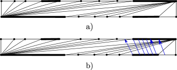
First, we briefly recall their complex, and refer the reader to [16] for more details. The street complex consists of a set of streets and junctions, which “bundle” common subpaths of the input curves . These are connected via their common boundary edges in the street complex, refer We model a street as a rectangle whose boundary is a simple cycle consisted of some vertices and edges. A generic street has two edges on the boundary that are segments of edges of , these are denoted by the in figure 2 a). The boundary minus and is divided into two paths that we call the sides of the street. In general, our model of a street is mapped to a street from [16] so that some pairs of the edges might identify with each other. Any pair of identified edges has one edge in each side. We draw these edges using a thick line. Figure 2 b) depicts a street model that is mapped to a spiral, shown in c).
The input compressed curve is a walk on the 1-skeleton of . We compute a straight-line program in Chomsky normal form for in polynomial time. The production rules with a terminal at the right-hand side now are of the form where is an oriented edge of the 1-skeleton of . We trace the multi-curve using the algorithm of [16], but at the same time define a composition system encoding the intersections of the edge with the street complex for We update the composition system after each step of the tracing algorithm, as described below.

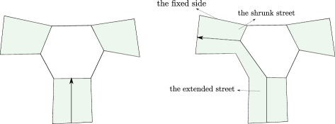
The basic step of the tracing algorithm is to extend a street across a junction or a fork, and then across a street. The extension across a junction and a street is depicted in Figure 3. This figure depicts a left turn across a junction. When a street is extended through a second street, the latter street is shrunk. When a street is shrunk, one side of the street remains unaltered, we call this side the fixed side of the street. The boundary of the street which is extended gains some new vertices and edges of the street complex, while the boundary of the street which is shrunk becomes simpler. A model the effect of this step on the streets is depicted in Figure 4.
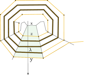
We next recall that a phase of the tracing algorithm of [16] consists of a maximal sequence of left turns or of right turns. When we enter a street for the second time, from the same side, during the same phase, we have discovered a spiral. In [16], they show that the spirals can be processed at once in time, where is the number of edges of ; see Figure 2. The presence of these spirals in a street causes potential identifications; we call the edge which is the result of an identification the long edge of the spiral. Observe that when another street extends over a street that contains a spiral, the latter street turns into an ordinary street without identifications. Since we are only interested in the case where is reduced, the complexity of the street complex is always bounded by a linear function of the complexity of [16, Lem. 2.3].
The terminals of are of three types: i) or , where is a street, is a vertex on , and is an edge of the street on the opposite side from , ii) where and are edges on opposite sides on the model of street , and iii) where and are vertices of the model street for lying on opposite sides. These three types of terminals represent sub-arcs of that lie inside the street, where the sub-arcs start at the second parameter and end at the third parameter. We use vertices and edges of the model street rather than the street itself. This allows us to distinguish between two arcs in the street complex, which have different directions, but connect the image of two edges or vertices that are identified in the street complex.

When traversing an edge of in the overlay of the street complex and the original complex , we see a sequence of these terminals which we call the overlay sequence of . Our first goal is to construct a composition system for the overlay sequence.
The algorithm that traces the curves in to build the street complex starts with the triangulation , where each edge is a (trivial) street and there is one fork where we start the tracing. At the beginning, we introduce for the edge of a non-terminal , where is the street of the edge . We also introduce the rule . This finishes the modifications for the starting street complex. We note that the composition system is not a well-defined until the algorithm is finished.
Assume that we turn right at a junction and let and be vertices of the street which is going to be shrunk, and be the right active street, as in the figure 4. If the non-terminal exists, we introduce the rule where is as in the figure. If the street coordinates of in (new) and/or in is 0, we also introduce terminals and the rule and/or . Similarly, if the non-terminal exists we introduce the rule We introduce also the suitable terminals in case any of the streets have coordinates zero for . Recall that during the tracing algorithm of [16], the number of arcs of inside each street is maintained as the street coordinates. If a street has 0 number of arcs of , it will not be shrunk again, and in this case we introduce the leafs of composition system.
Next, for any two vertices on different sides of the model street for , if the non-terminal exists, and lies on the fixed side of , we introduce the rule where is the edge of (new) street as in the figure 4. If the street coordinates of in and/or in is 0, we also introduce terminals and the rule and/or . Similarly, if the non-terminal exists where is on the fixed side of the street we introduce the rule We introduce also the suitable terminals in case any of the streets have coordinates zero for . This finishes the processing of non-terminals of type iii).
If is a non-terminal such that and lie on two sides of and lies on the fixed side of , we introduce new non-terminals and the rule , where is the new side of the shrunk street , as in the figure. We introduce new terminals if the coordinates are zero as above and do symmetrically if is on the fixed side of the street. This deals with the non-terminals of the second type. An analogous argument works for the non-terminals of the first type.
The modifications necessary for extension across a fork are totally analogous to a junction. In this case again a street is shrunk and another is extended, see [16] figure 7. We do not repeat the case analysis.
We next consider a spiral. Let be the depth of the spiral, the length of the spiral, and be the number of distinct streets traversed by the spiral. See [16] for more detailed description of these parameters and how to compute the spiral. Let be the long edge of the spiral, and , be its preimages in the model. After we enter a spiral and before we reach the ”final turn”, the new side of the shrunk street is always and the extended street has the edge on both sides. See figure 5. Let, in the system at the time we discover the spiral, be the non-terminal where is a street traversed by the spiral, and and be edges on its two sides such that lies on the fixed side of . After we trace the whole spiral, we need to add the rule , where is the active street. The number is either or depending on where the street lies around the spiral, in the example of figure 5 it is . In place of the star we place indices as is appropriate. If any street coordinate in the streets becomes zero we introduce the rule . If the active street has coordinates zero for we add the rule . We then extend the street through the streets that are traversed more than times. If is on the fixed side of the street we do analogously. We perform these modifications for every existing non-terminal of the form . This finished the modifications of the composition system for the non-terminals of type ii). Those of other two types are handled similarly.
We have finished the construction of the composition system . Note that since the curve is reduced no street is an annulus. At this stage of the argument, we have replaced each rule of the walk by a composition system encoding its overlay sequence with the street complex. To construct we do as follows. For each edge of the the street complex, we choose one of the two endpoints. We next replace the terminals of the system with a paths on the boundary of a street. This transforms the composition system into a composition system for the curve which is freely homotopic to , and is a walk on the 1-skeleton of the street complex.
Our next step is to triangulate the streets of the complex. For each street , we triangulate the street by adding diagonals as in the Figure 6 a). Let be a complex encoding this triangulation. is simply the collection of our street models, junctions and their edges and vertices where we identify edges that are identified in the street complex. There is a homeomorphism . By subdividing we can make sure that it is a simplicial complex. We also modify the composition system for to reflect the subdivision.
∎
Remark
The proof of Proposition 3 can also be used to construct the image in the triangulation as a hybrid compressed word whose terminals are either edges of the 1-skeleton, or arcs that connect a vertex to an edge or two edges in the same triangle. To compute we start again with the street complex and the composition systems . We add the diagonals again as in Figure 6 a) to obtain a complex . Replace each terminal of the form where and are (not necessarily) distinct edges of the street , by the sequence of intersections of the arc with the diagonals of . To find this sequence, we simply connect a points in the interior of to a point in the interior of by a direct line segment in our model street and replace with the sequence of intersections obtained, as in figure 6 b). We do this process analogously for other types of arcs, yielding the curve . The curve might be of independent interest for other problems.
5 Capping off
In this section, we show that the complex obtained by gluing disks on a family of disjoint curves on a surface is homotopy equivalent to a wedge of surfaces and circles. We provide a polynomial-time algorithm to compute the resulting wedge, while also tracking what happens to a compressed curve on the original surface.
Proposition 4.
Let be simplicial complex triangulating a surface of genus , be a family of disjoint embedded closed curves in the 1-skeleton of and be a compressed closed walk on the 1-skeleton of . The size of the input is the summation of the complexities of , and the number of edges of . We can compute in polynomial time a simplicial complex which is a wedge of surfaces and circles, and a compressed walk on , so that:
-
•
is homotopy equivalent to the complex obtained by gluing disks on each component of ,
-
•
is homotopic to a trivial walk in if and only if belongs to the normal subgroup determined by the curves in .
Proof.
Note that the second property will be satisfied if, in the complex satisfying the first property, we take for the image of under a homotopy equivalence of to . We construct the simplicial complex which is homotopy equivalent to the space obtained from by gluing a disk to each component of . This is done one disk at a time, and at each step we also maintain the image of the curve as a compressed word. Suppose has components. As a preprocessing step, we subdivide any edge that connects vertices on but does not lie on , twice, subdivide the incident triangles, and then update the compressed word.
Call a space a pinched surface if there is a finite set of vertices such that the closure of is a surface. We call the set of pinch points and assume is minimal, in the sense that is not homeomorphic to in any neighborhood of a point in .
We start by computing a straight-line program in Chomsky normal form for . During the procedure that processes components of , we maintain the following invariants: i) the current space is a pinched surface, ii) the current space is homotopy equivalent to union caps over components of that we have processed so far, iii) the current curve is the image of the original curve under a homotopy equivalence.
Let be a component of and let be the current complex. We add a disk with boundary ; we then compress this disk into a single vertex and add to . See Figure 7. The effect on the word is as follows. A terminal where is an edge in is replaced with . A terminal , where is in but is not, is replaced with . If is in and is not, the oriented edge is replaced with . We then remove all the sequences in the word . This can be accomplished in polynomial time. We note that each remaining component of is an embedded curve in the 1-skeleton lying in a single component of . The invariants remain true, and the word is now a walk in the new complex .
After contracting all the components of we have a complex which is a pinched surface. We transform into a homotopy equivalent surface by replacing each pinch point by a path of two edges where maps to under the homotopy equivalence that contracts We then compute a spanning tree of the vertices for . We require that the number of vertices is minimal in this tree. We then contract every edge of the spanning tree. The result is a complex which is wedge of circles and surfaces.
We explain the modifications needed to maintain the word . The first step is when we introduce the paths . Define , , and let denote the edges with the opposite orientation. Observe that the link of the vertex consists of two disjoint circles. We associate to one of these and to the other arbitrarily. If a terminal is an edge , where is in the circle associated to , we replace with the path , where . If is in the circle associated to , we replace with the path where . We do analogously for the edges of the form . These modifications define a curve which is the image of the homotopy equivalence which introduces the paths. It remains to update under contraction of a single edge. This is possible in polynomial time similar to contraction of a circle above. The result is the required curve .
∎
6 Triviality for compressed words in free products of surface groups
In this section, we prove the following theorem:
Theorem 4.
Let be a wedge of combinatorial surfaces and circles and be a compressed walk on . Then one can compute in polynomial time a canonical form for the homotopy class of . In particular, we can test in polynomial time whether is trivial.
We emphasize that in this theorem, we consider as a walk with fixed endpoints, and thus we are considering based homotopies (as opposed to free homotopies).
We can assume that there are no spheres in the wedge of surfaces: since these are simply connected, removing them, and replacing their edges by empty letters in the word does not change the homotopy class, or contractibility of . Furthermore, tori require a slightly different treatment from the other surfaces. For the ease of exposition, we first explain and justify our algorithm assuming that there are no tori in the wedge, and at the end of the proof we will explain how to deal with them.
Our algorithm starts in a similar way as the known linear-time algorithms to test contractibility or homotopy of curves on surfaces [17, 30]: we first turn each surface in the wedge into a system of quads (Lemma 2), and then compute a canonical form for our curve (Lemma 5). This canonical form is unique, and therefore the walk is homotopic to a trivial walk if and only if its reduced canonical form is the empty walk. However, due to the compression of the input, our techniques to reduce the curve are more involved than those of the aforementioned references.
Let denote the straight-line program encoding . First, we fix once and for all an orientation for all the surfaces in , which gives meaning to the intuitive notions of turning right, clockwise, etc.
Then our first step is to turn our surfaces into systems of quads. First, for each surface , we compute a spanning tree and contract it. Then, we remove edges until there is a single face, we add a new vertex inside the single face, add all the radial edges between this new vertex and the single vertex of and remove all the previous edges. To make things unified, in each circle summand, each loop is subdivided into two edges. The resulting complex is called a quad system.
Lemma 2.
Let be a wedge of surfaces and circles and let be a compressed walk on . In polynomial time we can turn into a quad system and compute a compressed walk on that is homotopic to .
Proof.
The construction of the quad system follows directly from the definition. The word is modified as follows: each terminal character representing an edge (which got removed) is now a non-terminal character with a production rule where is a two-edge path homotopic to going through the new middle vertex. On surfaces, there can be two such edge-paths, we choose arbitrarily. The other production rules are unchanged. This operation can be done in polynomial time and yields a compressed curve homotopic to . ∎
In the next step of our algorithm, we encode words using turn sequences. For any two directed edges and on the same surface , the turn is the number of corners, counted with respect to our chosen orientation, between the end of and the start of on . For any two edges and forming a loop in a circle summand, we define to be a new symbol , and for an edge in an circle summand, we define to be , which is in line with the case of surfaces. We need our encoding to adapt to jumps between different surfaces, and we do it as follows: If and are on different surfaces or circle summands, we define the turn to be the pair , with the intended meaning that in this case the turn is a jump from to on the new surface. Turn sequences are to be understood modulo the degree of the vertices, and following the literature, we use the notation . The symbol satisfies . Henceforth, by a slight abuse of language, we count circle summands among the surface since they will be treated the same way. The turn sequence of our word is the concatenation of all the turn sequences of consecutive edges. However, we lose information by encoding with turn sequences. First, a turn sequence does not specify a starting edge. Second, even if we know the starting edge, it is not immediately clear how to compute an arbitrary intermediate edge along the path efficiently since we encode exponential length paths. The following lemma shows how to do that in polynomial time.
Lemma 3.
Let be a compressed turn sequence and be an integer. Then if we are given a starting edge , then in polynomial time we can compute the edge of we are on just after starting at and following the turn sequence up to .
Proof.
We first compute a straight-line program for , then use Lemma 1 to compute the last letter of this word that corresponds to an edge. We denote it by , and if there is none we use instead. We denote by the index where it appears, which is if there is no such edge. Then we look at the straight-line program computing , which thus stays on a single surface. We inductively go up the production tree, computing, for each directed edge of the surface and for each production rule at which directed edge we arrive if we start at edge . This is straightforward at the leaves of the tree, and for a directed edge and a production rule of of the form , we can look up where we arrive after starting at and following , denote the resulting edge by , and then look up where we arrive after starting at and following . Finally, we obtain our solution by looking up where we are after starting at and following . ∎
The point of turn sequences is that they make it easier to make local simplifications to a contractible curve. Following Lazarus-Rivaud [30] and Erickson-Whittlesey [17], we use the following simplification rules, see Figure 8, which are homotopies.
-
•
A spur in a turn sequence is a turn. Removing a spur is applying the rule .
-
•
A bracket in a turn sequence is a subword of the form or . Flattening a bracket is applying the rules or .
We are only considering homotopies of paths in this paper, and thus do not need the other special cases considered in Erickson-Whittlesey [17]. Our goal is to modify the turn sequence so that it is reduced, i.e., contains neither spurs nor brackets. However, unlike in the aforementioned works, we cannot apply these rules directly, even inductively: in a production rule , even when and are reduced, there might be an exponential number of bracket flattenings in , for example in the cases in Figure 9.
There are known techniques to handle exponentially long spurs [32, 39], but for the more intricate cases pictured in Figure 9, especially the kind on the right side, we need to develop our own tools. In order to do that, we rely on stronger inductive forms, similarly to those used in the free homotopy test [17, 30]. A reduced path is leftmost (or rightmost, respectively) if its turn sequence contains no , respectively no (we emphasize that we also use this definition in our general setting of wedges of surfaces). Note that leftmost paths become rightmost paths under reversal, and vice-versa. This trivial observation will fuel many of our arguments. One can transform a reduced path into its rightmost (resp. leftmost) form by doing elementary right-shifts (resp. elementary left-shifts) which are the three transformations , and or their mirrors, see Figure 8.
For each character in the straight-line program, we inductively compute both a rightmost and leftmost turn sequence. Then, both are used to carry the induction step. So the next step of our algorithm is the following reduction algorithm. It takes as input the straight-line program describing a walk on a system of quads, and at the same time transforms it into two compressed turn sequences representing the reduced leftmost and rightmost form for the walk. In these representations, every character of encoding a walk gives rise to two characters and representing the turn sequences of the leftmost and rightmost form of . Since turn sequences only encode the turns at the interior vertices of a path and forget where the path starts, we store this information separately: for each character in the straight-line program, we store in a dictionary its starting and ending edges (which might be empty).
Reduction Algorithm
Input: A compressed walk on a quad system described by a straight-line program , as output by Lemma 2.
Output: Two compressed turn sequences on a quad system which are the leftmost and rightmost forms of the input, and their starting and ending edges.
-
•
The leaves of the production tree are transformed to empty sequences since they consist of a single edge. We store the edge as both the starting and the ending edge in our dictionary.
-
•
Let be a production rule, and assume that we have inductively computed rightmost and leftmost reduced turn sequences for and , which are denoted by , , and , as well as their starting and ending edges. We explain how to compute a rightmost reduced turn sequence , the leftmost case being symmetric. If the dictionary entries of and are empty, is an empty sequence, with empty starting and ending edges. If one of the dictionary entries is empty, is the other turn sequence, inheriting its starting and ending edges. Otherwise:
-
1.
We look up the last edge of and the first edge of in the dictionary and compute the turn between them 333At the start of steps 1, 2 and 3, it might happen that the last letter of and the first letter of are both edges, if half of a jumping turn got removed. In that case, we remove those edges since they are superfluous.. If it is different from or , we go to step 3. Otherwise, we use Lemma 1 to compute the largest so that if they have the same ending edge (let us emphasize that we use the leftmost form here). We use Lemma 3 to compute the last edge of . If it arrives at the same vertex as , we go to step 2 with and . If not, we go to step 2 with and , where is the turn .
- 2.
-
3.
If we came directly here, we look up the last edge of and the first edge of in the dictionary and compute the turn between them††footnotemark: . If we came from step 2, we compute††footnotemark: these edges using Lemma 3 and use them to compute . We concatenate the two words, adding in between.
-
a.
If , we use Lemma 1 to compute the maximal subword , and apply an elementary shift which changes it into , , , or depending on whether or is zero (if or are edges, they are changed into the turned edges). Since it is straightforward to encode efficiently using straight-line programs, this is done in polynomial time. We go to step b.
-
b.
If or , we use Lemma 1 to compute a maximal subword of the form . There might be multiple such subwords, we pick one of them arbitrarily. We change it into (if or are edges, they are changed into the turned edges). Since it is straightforward to encode efficiently using straight-line programs, this is done in polynomial time. We loop this step while there are brackets. When there are none, we output the result and store in our dictionary the first and last edge: these are the first and last edge of respectively, and , perhaps turned because of one of the elementary operations, or perhaps made empty if the entire word became empty.
-
c.
In any other case, we do not change anything and output the concatenated word, and store in our dictionary the first edge of and the last edge of .
-
a.
-
1.
Step 3 simply implements the bracket flattenings and the shifts, so the main mysteries in this algorithm are steps 1 and 2. These are tailored to deal with the bad cases pictured in Figure 9, which are the only possible bad cases; see the proof of Lemma 4. Figure 10 illustrates how step 1 reduces (a subset of) the right case of Figure 9 to its left case, and how step 2 deals with that case. Note that in these pictures, and were already rightmost.
We claim that after this procedure, the path that represents the word (respectively ) is homotopic to the path represented by , and is rightmost (respectively leftmost). This is straightforward for the leaves of the production tree, but the rest requires some more involved analysis.
For this analysis, we employ the terminology developed by Despré and Lazarus in their analysis of the combinatorics of quad systems [13, Section 4], to which we refer the reader for definitions. We will rely on two important structural results [13, Theorem 8 and Theorem 10](see also [17, 30]).
Theorem 5.
For a path on a combinatorial surface of negative Euler characteristic described by a system of quads, there is a unique rightmost, respectively leftmost, path homotopic to .
Theorem 6.
Let and be a rightmost and a leftmost path on a combinatorial surface of negative Euler characteristic described by a system of quads. Then bounds a disk diagram composed of an alternating sequence of paths and quad staircases connected through their tips.
The two theorems extend directly to our setting of wedge of surfaces and circles, since the fundamental group of a wedge of spaces is the free product of their fundamental groups. For the first theorem, the generalization to wedges then follows by the uniqueness of the rightmost and leftmost paths in each surface they span. For the second theorem, we obtain the generalization to wedges by gluing the disk diagrams in each surface together.
The following lemma is the crux of the analysis. We state it for rightmost paths but the symmetric version with leftmost paths holds with the same proof.
Lemma 4.
At the end of step 2, the paths represented by and are rightmost. Furthermore, denoting by the turn between and at the end of step 2, the path represented by is homotopic to the one before these two steps, contains no spurs, contains at most two brackets, and these brackets contain both at least one .
Proof.
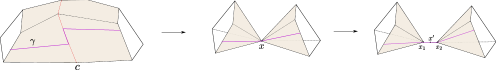
Since and are obtained from subpaths of rightmost curves, they are rightmost. Recall that is the rightmost path homotopic to . Since is homotopic to , the three paths represented by , and bound together a disk diagram. Since and are rightmost, by uniqueness of rightmost representatives of paths, they share a unique maximal subpath which is a common prefix, likewise for and where it is a common suffix. We consider the combinatorial triangle obtained after removing these subpaths, see Figure 11. We denote its endpoints by and , where is the vertex between and , the vertex between and , and the last one. Let denote the first vertex of degeneracy of on the path from to , and denote the vertex at the end of the first common path of and between and . Then we have a pinched disk diagram between and , the boundary of which is made of a subpath of and a subpath of . Theorem 6 tells us that this disk diagram is an alternating sequence of staircases and paths, which are connected by their tips. By definition, is the tip of a staircase. We claim that also lies on . Otherwise, denoting by and the leftmost paths between and and between and , the turn between and at would be , yielding a bracket with the other side of the staircase, a contradiction.
Since and are both rightmost, they have the same length and , the leftmost path homotopic to is exactly . Therefore, during Step 1., the whole subdisk between and got removed.
We denote by the disk diagram obtained after doing Step 1, with endpoints , and as before, and we distinguish cases depending on its orientation. If is degenerate, i.e., has no quads in its interior, then after removing possibly one sequence of spurs in step 2., we have and thus we have successfully computed a rightmost form for .
If the boundary of , oriented , is oriented clockwise, then is on the path between and , since and can not coincide below , see Figure 11, top. After removing the sequence of spurs between and in step 2., the turn between and is at least , since otherwise there would be a spur in or .
If the boundary of , oriented , is oriented counter-clockwise, we observe that also lies on . Indeed, otherwise, since is at distance at most one from and is not degenerate, there would be a common vertex that would be both on and and such that the paths from to are different, since one contains and not the other. This would contradict uniqueness of canonical paths. Therefore, the entire pinched disk between and has been removed in Step 1. Now we look at the maximal (possibly empty) staircase having as a tip and being bounded by pair of subpaths and of and , except for one edge. If there is no such staircase, nothing happens in step 2, and we are done. If there is such a staircase, we claim that most of it got already removed when we get to Step 2. If contains one or more s, then the start of the leftmost form of coincides with the start of , and thus this subword containing this has also been eliminated during step 1, see Figure 10. Note that the slight offset of the indices in Step 1 is due to the difference in length between and , and that the new turn that we introduce is the missing edge to close the staircase. Therefore, contains no , and the last turn of is a . Therefore the entire staircase is a ladder, as pictured in the left of Figure 9 and on the bottom right of Figure 11, which gets removed during step 2.
Let denote the turn between and after steps 1 and 2. Then in the clockwise case, is at least and thus at most one bracket can exist in . In the counter-clockwise case, the only brackets that can exist in must contain a , as otherwise the staircase of the previous paragraph would not have been maximal. There are at most two such brackets: one finishing at and one starting at , since otherwise such a bracket would have been present in or . As the reductions correspond to flattening brackets and removing spurs on a disk diagram, they are homotopies. Finally, since the degenerate parts of the disk diagram have been removed, there are no spurs. ∎
We now prove that the reduction algorithm does indeed compute rightmost and leftmost forms.
Lemma 5.
The Reduction Algorithm runs in polynomial time. The straight-line program that it outputs has the property that every pair of characters and encode a pair of turn sequence corresponding respectively to the rightmost and leftmost paths homotopic to . In particular, at the top level, and are the rightmost and leftmost paths homotopic to the compressed input walk.
Proof.
By Lemma 4, when the algorithm reaches step 3, the path may not be reduced for two reasons: either the turn between and is a , or there is one or two brackets with at least one between them. Note that the two cases are exclusive. We argue that no spurs or brackets remain after the two reductions a and b. For the first one (reduction a)), note that by definition and and are neither nor because is rightmost. We may have or , which may create at most two brackets, but note that these brackets are disjoint and contain each at least one .
When we reach step b, we therefore have at most two brackets, each containing at least one . We conclude by proving that no new brackets nor spurs are created during an application of this step b. Note that and cannot be because the curves are rightmost, cannot be because they contain no spurs, and cannot be because otherwise there would be a bracket without a . They could be , but the blocks the resulting from participating in a bracket since there is no torus surface among the wedge summands. Therefore, the only way for or to be involved in a bracket is if one of them is , in which case it bounds a second bracket that already existed before the reduction. After reducing that one, there are no more possible spurs nor brackets. In particular, step 3.b. only loops a constant number of times, and thus the whole inductive step is polynomial. In turn, computing the full straight-line programs for both reduced words and is also polynomial. ∎
We are now ready to prove Theorem 4.
Proof of Theorem 4.
Using Lemma 2, we first turn our walk into a walk on a quad system. Then, using Lemma 5, we compute a compressed rightmost loop homotopic to in this quad system. By Theorem 5, there is a unique such rightmost loop. Combined with the data of the first and last edge, this is our canonical form. If is homotopic to a trivial walk, it is homotopic to the empty loop, which is rightmost. Therefore, to test contractibility, it suffices to test whether is the empty word. ∎
Finally, let us comment on how to adapt this algorithm in the case where there are tori in the wedge. In tori summands, we dispense from using turn sequences and simply reduce to a one-vertex one-face graph, which therefore has two edges and . Homotopy in tori is a simple matter since the fundamental group is , corresponding exactly to how many times the oriented edges and are taken. Therefore, we directly use for our encoding a pair representing this, with the convention that . The reduction algorithm has an additional rule stipulating that should be reduced to . Any reduction to triggers a search for a deeper sequences of spurs and staircases as in Steps 1 to 3.
Proofs of the main theorems
We now have all the tools to prove our main theorems. Theorem 3 is a subcase of Theorem 4 when the the wedge of surfaces consists of a single surface.
Proof of Theorem 2.
We can make reduced in polynomial time [16]. By Proposition 3, one can compute in polynomial time a new triangulation of the surface so that the multi-curve has polynomial complexity and the curve is encoded as a straight-line program. By Proposition 4, we can compute a wedge of surfaces and circles and a walk on so that is contractible in if and only if belongs to the normal subgroup generated by the curves in . The simplicial complex can be transformed to a wedge of combinatorial surfaces and circles easily. Then the theorem follows from Theorem 4. ∎
Proof of Theorem 1.
By Proposition 2, we can reduce our problem to the case of orientable manifolds. Note that the size of the manifold at most doubles in this process. Then, Proposition 1 reduces the problem to the disjoint normal subgroup membership problem. The NP certificate consists of the certificate in that proposition, and the corresponding algorithm is to guess this certificate. The disjoint normal subgroup membership problem is then solved using Theorem 2. ∎
Acknowledgements
The authors would like to thank Mark Bell, Ben Burton, and Jeff Erickson for helpful discussions. We also thank an anonymous referee of [11] for suggesting the use of a maximal compression body as a simple exponential-time algorithm for deciding contractability of arbitrary (non-compressed) curves on the boundary of a 3-manifold.
References
- [1] Ian Agol, Joel Hass, and William Thurston. The computational complexity of knot genus and spanning area. Transactions of the American Mathematical Society, 358(9):3821–3850, 2006.
- [2] Matthias Aschenbrenner, Stefan Friedl, and Henry Wilton. Decision problems for 3–manifolds and their fundamental groups. Geometry & Topology Monographs, 19(1):201–236, 2015.
- [3] Matthias Aschenbrenner, Stefan Friedl, Henry Wilton, and Stefan Friedl. 3-manifold groups, volume 20. European Mathematical Society Zürich, 2015.
- [4] Mark C Bell. Simplifying triangulations. arXiv preprint arXiv:1604.04314, 2016.
- [5] Benjamin Burton, Éric Colin de Verdière, and Arnaud de Mesmay. On the complexity of immersed normal surfaces. Geometry & Topology, 20(2):1061–1083, 2016.
- [6] Benjamin A Burton. A new approach to crushing 3-manifold triangulations. Discrete & Computational Geometry, 52(1):116–139, 2014.
- [7] James W Cannon, David BA Epstein, Derek F Holt, Silvio VF Levy, Michael S Paterson, and William P Thurston. Word processing in groups. CRC Press, 1992.
- [8] Pierre de La Harpe. Topics in geometric group theory. University of Chicago Press, 2000.
- [9] Arnaud de Mesmay, Yo’av Rieck, Eric Sedgwick, and Martin Tancer. The Unbearable Hardness of Unknotting. In Gill Barequet and Yusu Wang, editors, 35th International Symposium on Computational Geometry (SoCG 2019), pages 49:1–49:19, Dagstuhl, Germany, 2019.
- [10] Éric Colin de Verdière and Salman Parsa. Deciding contractibility of a non-simple curve on the boundary of a 3-manifold. In Proceedings of the Twenty-Eighth Annual ACM-SIAM Symposium on Discrete Algorithms, pages 2691–2704. SIAM, 2017.
- [11] Éric Colin de Verdière and Salman Parsa. Deciding contractibility of a non-simple curve on the boundary of a 3-manifold: A computational loop theorem. arXiv preprint arXiv:2001.04747, 2020.
- [12] Max Dehn. Transformation der Kurven auf zweiseitigen Flächen. Mathematische Annalen, 72(3):413–421, 1912.
- [13] Vincent Despré and Francis Lazarus. Computing the geometric intersection number of curves. Journal of the ACM (JACM), 66(6):1–49, 2019.
- [14] Ivan Dynnikov. Counting intersections of normal curves. arXiv preprint arXiv:2010.01638, 2020.
- [15] Ivan Dynnikov and Bert Wiest. On the complexity of braids. Journal of the European Mathematical Society, 9:801–840, 2007.
- [16] Jeff Erickson and Amir Nayyeri. Tracing compressed curves in triangulated surfaces. Discrete and Computational Geometry, 49:823–863, 2013.
- [17] Jeff Erickson and Kim Whittlesey. Transforming curves on surfaces redux. In Proceedings of the twenty-fourth annual ACM-SIAM symposium on Discrete algorithms, pages 1646–1655. SIAM, 2013.
- [18] Christian Hagenah. Gleichungen mit regulären Randbedingungen über freien Gruppen, 2000.
- [19] Joel Hass, Jeffrey C Lagarias, and Nicholas Pippenger. The computational complexity of knot and link problems. Journal of the ACM (JACM), 46(2):185–211, 1999.
- [20] Joel Hass, Jack Snoeyink, and William P Thurston. The size of spanning disks for polygonal curves. Discrete and Computational Geometry, 29(1):1–18, 2003.
- [21] A. Hatcher, Cambridge University Press, and Cornell University. Department of Mathematics. Algebraic Topology. Algebraic Topology. Cambridge University Press, 2002.
- [22] John Hempel. 3-Manifolds, volume 349. American Mathematical Soc., 2004.
- [23] Derek Holt, Markus Lohrey, and Saul Schleimer. Compressed Decision Problems in Hyperbolic Groups. In Rolf Niedermeier and Christophe Paul, editors, 36th International Symposium on Theoretical Aspects of Computer Science (STACS 2019), volume 126, pages 37:1–37:16, Dagstuhl, Germany, 2019.
- [24] William Jaco and J. Hyam Rubinstein. 0-efficient triangulations of 3-manifolds. Journal of Differential Geometry, 65(1):61–168, 2003.
- [25] William Jaco and Jeffrey L Tollefson. Algorithms for the complete decomposition of a closed -manifold. Illinois journal of mathematics, 39(3):358–406, 1995.
- [26] Greg Kuperberg. Algorithmic homeomorphism of 3-manifolds as a corollary of geometrization. Pacific Journal of Mathematics, 301(1):189–241, 2019.
- [27] Marc Lackenby. The efficient certification of knottedness and Thurston norm. arXiv preprint arXiv:1604.00290, 2016.
- [28] Marc Lackenby. Some conditionally hard problems on links and 3-manifolds. Discrete & Computational Geometry, 58(3):580–595, 2017.
- [29] Marc Lackenby. Algorithms in 3-manifold theory. arXiv preprint arXiv:2002.02179, 2020.
- [30] Francis Lazarus and Julien Rivaud. On the homotopy test on surfaces. In 2012 IEEE 53rd Annual Symposium on Foundations of Computer Science, pages 440–449. IEEE, 2012.
- [31] Maarten Löffler, Anna Lubiw, Saul Schleimer, and Erin Moriarty Wolf Chambers. Computation in Low-Dimensional Geometry and Topology (Dagstuhl Seminar 19352). In Dagstuhl Reports, volume 9. Schloss Dagstuhl-Leibniz-Zentrum fuer Informatik, 2019.
- [32] Markus Lohrey. Word problems and membership problems on compressed words. SIAM Journal on Computing, 35(5):1210–1240, 2006.
- [33] Markus Lohrey. The compressed word problem for groups. Springer, 2014.
- [34] Sergei Vladimirovich Matveev. Algorithmic topology and classification of 3-manifolds, volume 9. Springer, 2007.
- [35] Bojan Mohar and Carsten Thomassen. Graphs on Surfaces. John Hopkins University Press, 2001.
- [36] Edwin E Moise. Affine structures in 3-manifolds: V. The Triangulation theorem and Hauptvermutung. Annals of mathematics, pages 96–114, 1952.
- [37] Marcus Schaefer, Eric Sedgwick, and Daniel Štefankovič. Algorithms for normal curves and surfaces. In International Computing and Combinatorics Conference, pages 370–380. Springer, 2002.
- [38] Marcus Schaefer, Eric Sedgwick, and Daniel Stefankovic. Computing Dehn twists and geometric intersection numbers in polynomial time. In CCCG, volume 20, pages 111–114. Citeseer, 2008.
- [39] Saul Schleimer. Polynomial-time word problems. Commentarii Mathematici Helvetici, 83:741–765, 2008.
- [40] Horst Schubert. Bestimmung der Primfaktorzerlegung von Verkettungen. Mathematische Zeitschrift, 76(1):116–148, 1961.
- [41] John Stillwell. Classical topology and combinatorial group theory, volume 72. Springer Science & Business Media, 2012.
- [42] Friedhelm Waldhausen. The word problem in fundamental groups of sufficiently large irreducible 3-manifolds. Annals of Mathematics, 88(2):272–280, 1968.