Figure 1. We devise a perceptually based model to optimize the error of Monte Carlo renderings. Here we show our vertical iterative minimization algorithm from Section 4.1: Given 4 input samples per pixel (spp), it selects a subset of them to produce an image with substantially improved visual fidelity over a simple 4-spp average. The optimization is guided by a surrogate image obtained by regularizing the noisy input; we also show using the ground-truth image as a guide. The power spectrum of the image error, computed on $32\!\times\!32$-pixel tiles, indicates that our method distributes pixel error with locally blue-noise characteristics.

Perceptual error optimization for Monte Carlo rendering

Abstract.

Synthesizing realistic images involves computing high-dimensional light-transport integrals. In practice, these integrals are numerically estimated via Monte Carlo integration. The error of this estimation manifests itself as conspicuous aliasing or noise. To ameliorate such artifacts and improve image fidelity, we propose a perception-oriented framework to optimize the error of Monte Carlo rendering. We leverage models based on human perception from the halftoning literature. The result is an optimization problem whose solution distributes the error as visually pleasing blue noise in image space. To find solutions, we present a set of algorithms that provide varying trade-offs between quality and speed, showing substantial improvements over prior state of the art. We perform evaluations using quantitative and error metrics, and provide extensive supplemental material to demonstrate the perceptual improvements achieved by our methods.

1. Introduction

Monte Carlo sampling produces approximation error. In rendering, this error can cause visually displeasing image artifacts, unless control is exerted over the correlation of the individual pixel estimates. A standard approach is to decorrelate these estimates by randomizing the samples independently for every pixel, turning potential structured artifacts into white noise.

In digital halftoning, the error induced by quantizing continuous-tone images has been studied extensively. Such studies have shown that a blue-noise distribution of the quantization error is perceptually optimal [Ulichney, 1987], achieving substantially higher image fidelity than a white-noise distribution. Recent works have proposed empirical means to transfer these ideas to image synthesis [Georgiev and Fajardo, 2016; Heitz and Belcour, 2019; Heitz et al., 2019; Ahmed and Wonka, 2020]. Instead of randomizing the pixel estimates, these methods introduce negative correlation between neighboring pixels, exploiting the local smoothness in images to push the estimation error to the high-frequency spectral range.

We propose a theoretical formulation of perceptual error for image synthesis which unifies prior methods in a common framework and formally justifies the desire for blue-noise error distribution. We extend the comparatively simpler problem of digital halftoning [Lau and Arce, 2007] where the ground-truth image is given, to the substantially more complex one of rendering where the ground truth is the sought result and thus unavailable. Our formulation bridges the gap between multi-tone halftoning and rendering by interpreting Monte Carlo estimates for a pixel as its admissible ‘quantization levels’. This insight allows virtually any halftoning method to be adapted to rendering. We demonstrate this for the three main classes of halftoning algorithms: dither-mask halftoning, error diffusion halftoning, and iterative energy minimization halftoning.

Existing methods [Georgiev and Fajardo, 2016; Heitz and Belcour, 2019; Heitz et al., 2019] can be seen as variants of dither-mask halftoning. They distribute pixel error according to masks that are optimized w.r.t. a target kernel, typically a Gaussian. The kernel can be interpreted as an approximation to the human visual system’s point spread function [Daly, 1987; Pappas and Neuhoff, 1999]. We revisit the kernel-based perceptual model from halftoning [Sullivan et al., 1991; Analoui and Allebach, 1992; Pappas and Neuhoff, 1999] and adapt it to rendering. The resulting energy can be directly used for optimizing Monte Carlo error distribution without the need for a mask. This formulation help us expose the underlying assumptions of existing methods and quantify their limitations. In summary:

• We formulate an optimization problem for rendering error by leveraging kernel-based perceptual models from halftoning.

• Our formulation unifies prior blue-noise error distribution methods and makes all their assumptions explicit, outlining general guidelines for devising new methods in a principled manner.

• Unlike prior methods, our formulation simultaneously optimizes for both the magnitude and the image distribution of pixel error.

• We devise four different practical algorithms based on iterative minimization, error diffusion, and dithering from halftoning.

• We demonstrate substantial visual improvements over prior art, while using the same input rendering data.

2. Related Work

Our work focuses on reducing and optimizing the distribution of Monte Carlo pixel-estimation error. In this section we review prior work with similar goals in digital halftoning (Section 2.1) and image synthesis guided by energy-based (Section 2.2) and perception-based (Section 2.3) error metrics. We achieve error reduction through careful sample placement and processing, and discuss related rendering approaches (Section 2.4).

2.1. Digital halftoning

Digital halftoning [Lau and Arce, 2007] involves creating the illusion of continuous-tone images through the arrangement of binary elements; various algorithms target different display devices. Bayer [1973] developed the widely used dispersed-dot ordered-dither patterns. Allebach and Liu [1976] introduced the use of randomness in clustered-dot ordered dithering. Ulichney [1987] introduced blue-noise patterns that yield better perceptual quality, and Mitsa and Parker [1991] mimicked those patterns to produce dither arrays (i.e., masks) with high-frequency characteristics. Sullivan et al. [1991] developed a Fourier-domain energy function to obtain visually optimal halftone patterns; the optimality is defined w.r.t. computational models of the human visual system. Analoui and Allebach [1992] devised a practical algorithm for blue-noise dithering through a spatial-domain interpretation of Sullivan et al.’s model. Their approach was later refined by Pappas and Neuhoff [1999].

The void-and-cluster algorithm [Ulichney, 1993] uses a Gaussian kernel to create dither masks with isotropic blue-noise distribution. This approach has motivated various structure-aware halftoning algorithms in graphics [Ostromoukhov, 2001; Pang et al., 2008; Chang et al., 2009]. In the present work, we leverage the kernel-based model [Analoui and Allebach, 1992; Pappas and Neuhoff, 1999] in the context of Monte Carlo rendering [Kajiya, 1986].

2.2. Quantitative error assessment in rendering

It is convenient to measure the error of a rendered image as a single value; vector norms like the mean squared error (MSE) are most commonly used. However, it is widely acknowledged that such simple metrics do not accurately reflect visual quality as they ignore the perceptually important spatial arrangement of pixels. Various theoretical frameworks have been developed in the spatial [Niederreiter, 1992; Kuipers and Niederreiter, 1974] and Fourier [Singh et al., 2019] domains to understand the error reported through these metrics. The error spectrum ensemble [Celarek et al., 2019] measures the frequency-space distribution of the error.

Many denoising methods [Zwicker et al., 2015] employ the aforementioned metrics to obtain noise-free results from noisy renderings. Even if the most advanced denoising techniques driven by such metrics can efficiently steer adaptive sampling [Chaitanya et al., 2017; Kuznetsov et al., 2018; Kaplanyan et al., 2019], they locally determine the number of samples per pixel, ignoring the aspect of their specific layout in screen space.

Our optimization framework employs a perceptual MSE-based metric that accounts for both the magnitude and the spatial distribution of pixel-estimation error. We argue that the spatial sample layout plays a crucial role in the perception of a rendered image; the most commonly used error metrics do not capture this aspect.

2.3. Perceptual error assessment in rendering

The study of the human visual system (HVS) is still ongoing, and well understood are mostly the early stages of the visual pathways from the eye optics, through the retina, to the visual cortex. This limits the scope of existing HVS computational models used in imaging and graphics. Such models should additionally be computationally efficient and generalize over the simplistic stimuli that have been used in their derivation through psychophysical experiments.

Contrast sensitivity function

The contrast sensitivity function (CSF) is one of the core HVS models that fulfills the above conditions and comprehensively characterizes overall optical [Westheimer, 1986; Deeley et al., 1991] and neural [Souza et al., 2011] processes in detecting contrast visibility as a function of spatial frequency. While originally modeled as a band-pass filter [Barten, 1999; Daly, 1992], the CSF’s shape changes towards a low-pass filter with retinal eccentricity [Robson and Graham, 1981; Peli et al., 1991] and reduced luminance adaptation in scotopic and mesopic levels [Wuerger et al., 2020]. Low-pass characteristics are also inherent for chromatic CSFs [Mullen, 1985; Wuerger et al., 2020; Bolin and Meyer, 1998]. In many practical imaging applications, e.g., JPEG compression [Rashid et al., 2005], rendering [Ramasubramanian et al., 1999], or halftoning [Pappas and Neuhoff, 1999], the CSF is modeled as a low-pass filter, which also allows for better control of image intensity. By normalizing such a CSF by the maximum contrast-sensitivity value, a unitless function akin to the modulation transfer function (MTF) can be derived [Daly, 1987; Mannos and Sakrison, 1974; Mantiuk et al., 2005; Sullivan et al., 1991; Souza et al., 2011] that after transforming from the frequency to the spatial domain results in the point spread function (PSF) [Analoui and Allebach, 1992; Pappas and Neuhoff, 1999]. Following Pappas and Neuhoff [1999], we approximate such a PSF by a Gaussian filter; the resulting error is practically negligible for a pixel density of 300 dots per inch (dpi) and observer-to-screen distance larger than 60 cm.

Advanced quality metrics

More costly, and often less robust, modeling of the HVS beyond the CSF is performed in advanced quality metrics [Lubin, 1995; Daly, 1992; Mantiuk et al., 2011]. Such metrics have been adapted to rendering to guide the computation to image regions where the visual error is most strongly perceived [Bolin and Meyer, 1995, 1998; Ramasubramanian et al., 1999; Ferwerda et al., 1996; Myszkowski, 1998; Volevich et al., 2000]. An important application is visible noise reduction in path tracing via content-adaptive sample-density control [Bolin and Meyer, 1995, 1998; Ramasubramanian et al., 1999]. Our framework enables significant reduction of noise visibility for the same sampling budget.

2.4. Blue-noise error distribution in rendering

Mitchell [1991] first observed that high-frequency error distribution is desirable for stochastic rendering. Only recently, Georgiev and Fajardo [2016] adopted techniques from halftoning to correlate pixel samples in screen space and distribute path-tracing error as blue noise, with substantial perceptual quality improvements. Heitz et al. [2019] built on this idea to develop a progressive quasi-Monte Carlo sampler that further improves quality. Ahmed and Wonka [2020] proposed a technique to coordinate quasi-Monte Carlo samples in screen space inspired by error diffusion.

Motivated by the results of Georgiev and Fajardo [2016], Heitz and Belcour [2019] devised a method to directly optimize the distribution of pixel estimates, without operating on individual samples. Their pixel permutation strategy fits the initially white-noise pixel intensities to a prescribed blue-noise mask. This approach scales well with sample count and dimension, though its reliance on prior pixel estimates makes it practical only for animation rendering where it is susceptible to quality degradation.

We propose a perceptual error framework that unifies these two general approaches, exposing the assumptions of existing methods and providing guidelines to alleviate some of their drawbacks.

3. Perceptual error model

Our aim is to produce Monte Carlo renderings that, at a fixed sampling rate, are perceptually as close to the ground truth as possible. This goal requires formalizing the perceptual image error along with an optimization problem that minimizes it. In this section, we build a perceptual model upon the extensive studies done in the halftoning literature. We will discuss how to efficiently solve the resulting optimization problem in Section 4.

Given a ground-truth image $\boldsymbol{I}$ and its quantized or stochastic approximation $\boldsymbol{Q}$, we denote the (signed) error image by

(1) $$\boldsymbol{\epsilon}=\boldsymbol{Q}-\boldsymbol{I}.$$

To minimize the error, it is convenient to quantify it as a single value. A common approach is to take the $\mathcal{L}_{1}$, $\mathcal{L}_{2}$, or $\mathcal{L}_{\infty}$ norm of the image $\boldsymbol{\epsilon}$ interpreted as a vector. Such simple metrics are permutation-invariant, i.e., they account for the magnitudes of individual pixel errors but not for their distribution over the image. This distribution is an important factor for the perceived fidelity, since contrast perception is an inherently spatial characteristic of the HVS (Section 2.3). Our model is based on perceptual halftoning metrics that capture both the magnitude and the distribution of error.

Image	Image spectrum	Kernel spectrum	Product spectrum
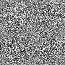
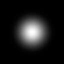
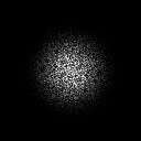
${\boldsymbol{\epsilon}_{\mathrm{w}}}$	$\left|{\hat{\boldsymbol{\epsilon}}}_{\mathrm{w}}\right|^{2}$	$\left|\hat{\boldsymbol{g}}\right|^{2}$	$\left|\hat{\boldsymbol{g}}\right|^{2}\odot\left|{\hat{\boldsymbol{\epsilon}}}_{\mathrm{w}}\right|^{2}$
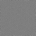
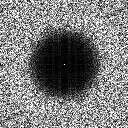
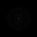
${\boldsymbol{\epsilon}_{\mathrm{b}}}$	$\left|{\hat{\boldsymbol{\epsilon}}}_{\mathrm{b}}\right|^{2}$	$\left|\hat{\boldsymbol{g}}\right|^{2}$	$\left|\hat{\boldsymbol{g}}\right|^{2}\odot\left|{\hat{\boldsymbol{\epsilon}}}_{\mathrm{b}}\right|^{2}$

Figure 2. Error images $\boldsymbol{\epsilon}_{\mathrm{w}}$ and $\boldsymbol{\epsilon}_{\mathrm{b}}$ with respective white-noise, $\left|{\hat{\boldsymbol{\epsilon}}}_{\mathrm{w}}\right|^{2}$, and blue-noise, $\left|{\hat{\boldsymbol{\epsilon}}}_{\mathrm{b}}\right|^{2}$, power spectra. For a low-pass kernel $\boldsymbol{g}$ modeling the PSF of the HVS (here a Gaussian with std. dev. $\sigma=1$), the product of its spectrum $\left|\hat{\boldsymbol{g}}\right|^{2}$ with $\left|{\hat{\boldsymbol{\epsilon}}}_{\mathrm{b}}\right|^{2}$ has lower magnitude than the product with $\left|{\hat{\boldsymbol{\epsilon}}}_{\mathrm{w}}\right|^{2}$. This corresponds to lower perceptual sensitivity to $\boldsymbol{\epsilon}_{\mathrm{b}}$, even though $\boldsymbol{\epsilon}_{\mathrm{w}}$ has the same amplitude as it is obtained by randomly permuting the pixels of $\boldsymbol{\epsilon}_{\mathrm{b}}$.

3.1. Motivation

Halftoning metrics model the processing done by the HVS as a convolution of the error image $\boldsymbol{\epsilon}$ with a kernel $\boldsymbol{g}$:

(2) $$E\,=\,\lVert\boldsymbol{g}*\boldsymbol{\epsilon}\rVert^{2}_{2}\,=\,\lVert\hat{\boldsymbol{g}}\,\odot\,\hat{\boldsymbol{\epsilon}}\rVert^{2}_{2}\,=\,\langle\left|\hat{\boldsymbol{g}}\right|^{2}\!\!,\,\left|\hat{\boldsymbol{\epsilon}}\right|^{2}\rangle.$$

The convolution is equivalent to the element-wise product of the corresponding Fourier spectra $\hat{\boldsymbol{g}}$ and $\hat{\boldsymbol{\epsilon}}$, whose 2-norm in turn equals the inner product of the power spectra images $\left|\hat{\boldsymbol{g}}\right|^{2}$ and $\left|\hat{\boldsymbol{\epsilon}}\right|^{2}$. Sullivan et al. [1991] optimized the error image $\boldsymbol{\epsilon}$ to minimize the error (2) w.r.t. a kernel $\boldsymbol{g}$ that approximates the HVS’s modulation transfer function $\left|\hat{\boldsymbol{g}}\right|$ (MTF) [Daly, 1987]. Analoui and Allebach [1992] used a similar model in the spatial domain with a kernel that approximates the PSF of the human eye. That kernel is low-pass, and the optimization naturally yields blue-noise distribution in the error image [Analoui and Allebach, 1992], as we show later in Fig. 5. The blue-noise distribution can thus be seen as byproduct of the optimization which pushes the spectral components of the error to the frequencies least visible to the human eye (see Fig. 2).

To better understand the spatial aspects of contrast sensitivity in the HVS, the MTF is usually modeled over a range of viewing distances [Daly, 1992]. This is done to account for the fact that with increasing viewer distance, spatial frequencies in the image are projected to higher spatial frequencies onto the retina. These frequencies eventually become invisible, filtered out by the PSF which expands its corresponding kernel in image space. We recreate this experiment to see the impact of distance on the image error. In Fig. 3, we convolve white- and blue-noise distributions with a Gaussian kernel of increasing standard deviation corresponding to increasing observer-to-screen distance. The high-frequency blue-noise distribution reaches a homogeneous state (where the tone appears constant) faster compared to the all-frequency white noise. This means that high-frequency error becomes indiscernible at closer viewing distances, where the HVS ideally has not yet started filtering out actual image detail which is typically low- to mid-frequency. In Section 6 we discuss how the kernel’s standard deviation encodes the viewing distance w.r.t. to the screen resolution.

$\sigma=0$	$\sigma=0.25$	$\sigma=0.5$	$\sigma=1$

Figure 3. The appearance of blue noise (left images) converges to a constant image faster than white noise (right images) with increasing observer distance, here emulated via the standard deviation $\sigma$ of a Gaussian kernel. We provide a formal connection between $\sigma$ and the viewing distance in Section 6.

3.2. Our model

In rendering, the value of each pixel $i$ is a light-transport integral. Point-sampling its integrand with a sample set $S$ yields a pixel estimate $Q_{i}(S)$. The signed pixel error is thus a function of the sample set: $\epsilon_{i}(S)=Q_{i}(S)-I_{i}$, where $I_{i}$ is the reference (i.e., ground-truth) pixel value. The error of the entire image can be written as

(3) $$\boldsymbol{\epsilon}(\boldsymbol{S})=\boldsymbol{Q}(\boldsymbol{S})-\boldsymbol{I},$$

where $\boldsymbol{S}=\{S_{1},\ldots,S_{N}\}$ is an “image” containing the sample set for all $N$ pixels. With these definitions, we can express the perceptual error in Eq. 2 for the case of Monte Carlo rendering as a function of the sample-set image $\boldsymbol{S}$, given a kernel $\boldsymbol{g}$:

(4) $$E(\boldsymbol{S})=\lVert\boldsymbol{g}*\boldsymbol{\epsilon}(\boldsymbol{S})\rVert_{2}^{2}.$$

Our goal is to minimize the perceptual error (4). We formulate this task as an optimization problem:

The minimizing sample-set image $\boldsymbol{S}$ yields an image estimate $\boldsymbol{Q}(\boldsymbol{S})$ that is closest to the reference $\boldsymbol{I}$ w.r.t. the kernel $\boldsymbol{g}$. The search space $\boldsymbol{\Omega}$ is the set of all possible locations for every sample of every pixel. The total number of samples in $\boldsymbol{S}$ is typically bounded by a given target sampling budget. Practical considerations may also restrict the search space $\boldsymbol{\Omega}$, as we will exemplify in the following section.

Note that the classical MSE metric corresponds to using a zero-width (i.e., one-pixel) kernel $\boldsymbol{g}$ in Eq. 4. However, the MSE accounts only for the magnitude of the error $\boldsymbol{\epsilon}$, while using wider kernels (such as the PSF) accounts for both magnitude and distribution. Consequently, while the MSE can be minimized by optimizing pixels independently, minimizing the perceptual error requires coordination between pixels. In the following section, we devise strategies for solving this optimization problem.

4. Discrete optimization

In our optimization problem (5), the search space for each sample in every pixel is a high-dimensional unit hypercube. Every point in this so-called primary sample space maps to a light-transport path in the scene [Pharr et al., 2016]. Optimizing for the sample-set image $\boldsymbol{S}$ thus entails evaluating the contributions $\boldsymbol{Q}(\boldsymbol{S})$ of all corresponding paths. This evaluation is costly, and for any non-trivial scene, $\boldsymbol{Q}$ is a function with complex shape and many discontinuities. This precludes us from studying all (uncountably infinite) sample locations in practice.

To make the problem tractable, we restrict the search in each pixel to a finite number of (pre-defined) sample sets. We devise two variants of the resulting discrete optimization problem, which differ in their definition of the global search space $\boldsymbol{\Omega}$. In the first variant, each pixel has a separate list of sample sets to choose from (“vertical” search space). The setting is similar to that of (multi-tone) halftoning [Lau and Arce, 2007], which allows us to import classical optimization techniques from that field, such as iterative minimization, error diffusion, and mask-based dithering. In the second variant, each pixel has one associated sample set, and the search space comprises permutations of these assignments (“horizontal” search space). We develop a greedy iterative optimization method for this second variant.

In contrast to halftoning, in our setting the ground-truth image $\boldsymbol{I}$—required to compute the error image $\boldsymbol{\epsilon}$ during optimization—is not readily available. Below we describe our algorithms assuming the ground truth is available; in Section 5 we will discuss how to substitute it with a surrogate to make the algorithms practical.

4.1. Vertical search space

Our first variant considers a “vertical” search space where the sample set for each of the $N$ image pixels is one of $M$ given sets:

(6) $$\boldsymbol{\Omega}=\left\{\boldsymbol{S}=\{S_{1},\ldots,S_{N}\}:S_{i}\in\{S_{i,1},\ldots,S_{i,M}\}\right\}.$$

The objective is to find a sample set $S_{i}$ for every pixel $i$ such that all resulting pixel estimates together minimize the perceptual error (4).

\begin{overpic}[abs,unit=0.25mm,scale={0.64}]{figures/vertical-search-space.ai} \put(161.0,55.0){\small\contourlength{0.55pt}\contour{black}{{\color[rgb]{1,1,1}$O_{1}$}}} \put(45.5,59.0){\small\contourlength{0.55pt}\contour{black}{{\color[rgb]{1,1,1}$Q_{1,M}$}}} \put(156.0,23.5){\small\contourlength{0.55pt}\contour{black}{{\color[rgb]{1,1,1}$O_{2}$}}} \put(34.0,5.0){\small\contourlength{0.55pt}\contour{black}{{\color[rgb]{1,1,1}$Q_{2,1}$}}} \put(126.0,18.5){\small\contourlength{0.55pt}\contour{black}{{\color[rgb]{1,1,1}$O_{3}$}}} \put(4.0,20.0){\small\contourlength{0.55pt}\contour{black}{{\color[rgb]{1,1,1}$Q_{3,2}$}}} \end{overpic}

This is equivalent to directly optimizing over the $M$ possible estimates $Q_{i,1},\ldots,Q_{i,M}$ for each pixel, with $Q_{i,j}=Q_{i}(S_{i,j})$. These estimates can be obtained by pre-rendering a stack of $M$ images $\boldsymbol{Q}_{j}=\{Q_{1,j},\ldots,Q_{N,j}\}$, for $j=1..M$. The resulting minimization problem reads:

(7) $$\min_{\boldsymbol{O}\,:\,O_{i}\in\,\{Q_{i,1},\ldots,Q_{i,M}\}}\lVert\boldsymbol{g}*(\boldsymbol{O}-\boldsymbol{I})\rVert^{2}_{2}.$$

This problem is almost identical to that of multi-tone halftoning. The difference is that in our setting the “quantization levels”, i.e., the pixel estimates, are distributed non-uniformly and vary per pixel as they are not fixed but are the result of point-sampling a light-transport integral. This similarity allows us to directly apply existing optimization techniques from halftoning. We consider three such methods, which we outline in Alg. 1 and describe next.

Iterative minimization

State-of-the-art halftoning methods attack the problem (7) directly via greedy iterative minimization [Analoui and Allebach, 1992; Pappas and Neuhoff, 1999]. After initializing every pixel to a random quantization level, we traverse the image in serpentine order (as is standard practice in halftoning) and for each pixel choose the level that minimizes the energy. Several full-image iterations are performed; in our experiments convergence to a local minimum is achieved within 10–20 iterations.

As a further improvement, the optimization can be terminated when no pixels are updated within one full iteration, or when the perceptual-error reduction rate drops below a certain threshold. Traversing the pixels in random order allows terminating at any point but converges slightly slower.

Error diffusion

A classical halftoning algorithm, error diffusion scans the image pixel by pixel, snapping each reference value to the closest quantization level and distributing the resulting pixel error to yet-unprocessed nearby pixels according to a given kernel $\boldsymbol{\kappa}$. We use the empirically derived kernel of Floyd and Steinberg [1976] which has been shown to produce an output that approximately minimizes Eq. 7 [Hocevar and Niger, 2008]. Error diffusion is faster than iterative minimization but yields less optimal solutions.

Dithering

The fastest halftoning approach quantizes pixel values using thresholds stored in a pre-computed dither mask (or matrix) [Spaulding et al., 1997]. For each pixel, the two quantization levels that tightly envelop the reference value (in terms of brightness) are found, and one of the two is chosen based on the threshold assigned to the pixel by the mask.

Dithering can be understood as performing the perceptual error minimization in two steps. First, an offline optimization encodes the error distribution optimal for the target kernel $\boldsymbol{g}$ into a mask. Then, for a given image, the error magnitude is minimized by restricting the quantization to the two closest levels per pixel, and the mask-driven choice between them applies the target distribution of error.

List of pseudocodes 1 Three algorithms to (approximately) solve the vertical search space optimization problem (7). The output is an image $\boldsymbol{O}=\{O_{1},\ldots,O_{N}\}$, given a reference image $\boldsymbol{I}$ and a stack of initial image estimates $\boldsymbol{Q}_{1},\ldots,\boldsymbol{Q}_{M}$. Iterative minimization updates pixels repeatedly, for each selecting the estimate that minimizes the perceptual error (4). Error diffusion quantizes each pixel to the closest estimate, distributing the error to its neighbors based on a kernel $\boldsymbol{\kappa}$. Dithering quantizes each pixel in $\boldsymbol{I}$ based on thresholds looked up in a dither mask $\boldsymbol{B}$ (optimized w.r.t. the kernel $\boldsymbol{g}$).

 

1:*function IterativeMinimization($\boldsymbol{g}$, $\boldsymbol{I}$, $\boldsymbol{Q}_{1}$, …, $\boldsymbol{Q}_{M}$, $\boldsymbol{O}$, $T$)

2:*   $\boldsymbol{O}=\{Q_{1,\text{rand}},\ldots,Q_{N,\text{rand}}\}$ $\leftarrow$ Init each pixel to random estimate

3:*   for $T$ iterations do

4:*      for pixel $i=1..N$ do $\leftarrow$ E.g., random or serpentine order

5:*        for estimate $Q_{i,j}\in\{Q_{i,1},\ldots,Q_{i,M}\}$ do

6:*           if $O_{i}==Q_{i,j}$ reduces $\lVert\boldsymbol{g}*(\boldsymbol{O}-\boldsymbol{I})\rVert_{2}^{2}$ then

7:*             $O_{i}=Q_{i,j}$ $\leftarrow$ Update estimate                             

8:*function ErrorDiffusion($\boldsymbol{\kappa}$, $\boldsymbol{I}$, $\boldsymbol{Q}_{1}$, …, $\boldsymbol{Q}_{M}$, $\boldsymbol{O}$)

9:*   $\boldsymbol{O}=\boldsymbol{I}$ $\leftarrow$ Initialize solution to reference

10:*   for pixel $i=1..N$ do $\leftarrow$ E.g., serpentine order

11:*      $O_{i}^{\text{old}}=O_{i}$

12:*      $O_{i}\in\operatorname*{arg\,min}_{Q_{i,j}}\lVert O_{i}^{\text{old}}-Q_{i,j}\rVert^{2}_{2}$

13:*      $\epsilon_{i}=O_{i}^{\text{old}}-O_{i}$ $\rcurvearrowsw$ Diffuse error $\epsilon_{i}$ to yet-unprocessed neighbors

14:*      for unprocessed pixel $k$ within support of $\boldsymbol{\kappa}$ around $i$ do

15:*        $O_{k}\mathrel{{+}{=}}\epsilon_{i}\cdot\kappa_{k-i}$          

16:*function Dithering($\boldsymbol{B}$, $\boldsymbol{I}$, $\boldsymbol{Q}_{1}$, …, $\boldsymbol{Q}_{M}$, $\boldsymbol{O}$)

17:*   for pixel $i=1..N$ do $\rcurvearrowsw$ Find tightest interval $[Q_{i}^{\text{low}},Q_{i}^{\text{high}}]$

18:*      $Q_{i}^{\text{lower}}=\arg\max_{Q_{i,j}\,:\,|Q_{i,j}|\,\leq\,|I_{i}|}|Q_{i,j}|$  containing $I_{i}$

19:*      $Q_{i}^{\text{upper}}=\operatorname*{arg\,min}_{\,Q_{i,j}\,:\,|Q_{i,j}|\,>\,|I_{i}|}|Q_{i,j}|$

20:*      if $|I_{i}|-|Q_{i}^{\text{lower}}|\,<\,B_{i}\cdot\big{(}|Q_{i}^{\text{upper}}|-|Q_{i}^{\text{low}}|\big{)}$ then

21:*        $O_{i}=Q_{i}^{\text{lower}}$ $\rcurvearrowne$  Set $O_{i}$ to $Q_{i}^{\text{lower}}$ or $Q_{i}^{\text{upper}}$ using threshold $B_{i}$

22:*      else

23:*        $O_{i}=Q_{i}^{\text{upper}}$          

 

4.2. Horizontal search space

We now describe the second, “horizontal” discrete variant of our minimization formulation (5). It considers a single sample set $S_{i}$ assigned to each of the $N$ pixels, all represented together as a sample-set image $\boldsymbol{S}$. The search space comprises all possible permutations $\Pi(\boldsymbol{S})$ of these assignments:

(8) $$\boldsymbol{\Omega}=\Pi(\boldsymbol{S}),\;\text{with}\;\,\boldsymbol{S}=\{S_{1},\ldots,S_{N}\}.$$

The goal is to find a permutation $\pi(\boldsymbol{S})$ that minimizes the perceptual error (4). The optimization problem (5) thus takes the form

(9) $$\min_{\pi\in\,\Pi(\boldsymbol{S})}\lVert\boldsymbol{g}*(\boldsymbol{Q}(\pi(\boldsymbol{S}))-\boldsymbol{I})\rVert^{2}_{2}.$$

We can explore the permutation space $\Pi(\boldsymbol{S})$ by swapping the sample-set assignments between pixels. The minimization requires

updating the image estimate $\boldsymbol{Q}(\pi(\boldsymbol{S}))$ for each permutation $\pi(\boldsymbol{S})$, i.e., after every swap. Such updates are costly as they involve re-sampling both pixels in each of potentially millions of swaps. We need to eliminate these extra rendering invocations during the optimization to make it practical. To that end, we observe that for pixels solving similar light-transport integrals, swapping their sample sets gives a similar result to swapping their estimates. We therefore restrict the search space to permutations that can be generated through swaps between such (similar) pixels. This enables an efficient optimization scheme that directly swaps the pixel estimates of an initial rendering $\boldsymbol{Q}(\boldsymbol{S})$.

Error decomposition

Formally, we express the estimate produced by a sample-set permutation in terms of permuting the pixels of the initial rendering: $\boldsymbol{Q}(\pi(\boldsymbol{S}))=\pi(\boldsymbol{Q}(\boldsymbol{S}))+\boldsymbol{\Delta}(\pi)$. The error $\boldsymbol{\Delta}$ is zero when the swapped pixels solve the same integral. Substituting into Eq. 9, we can approximate the perceptual error by (see Appendix A)

(10a) $$\!\!E(\pi) =\lVert\boldsymbol{g}*(\pi(\boldsymbol{Q}(\boldsymbol{S}))-\boldsymbol{I}\,+\,\boldsymbol{\Delta}(\pi))\rVert^{2}_{2}$$

(10b) $$\approx\lVert\boldsymbol{g}*(\pi(\boldsymbol{Q}(\boldsymbol{S}))-\boldsymbol{I})\rVert^{2}_{2}\,+\lVert\boldsymbol{g}\rVert^{2}_{1}\sum_{i}d(i,\pi(i))=E_{d}(\pi),\,\,$$

where we write the error $E(\pi)$ as a function of $\pi$ only, to emphasize that everything else is fixed during the optimization. In the approximation $E_{d}$, the term $d(i,\pi(i))$ measures the dissimilarity between pixel $i$ and the pixel $\pi(i)$ it is relocated to by the permutation. The purpose of this metric is to predict how different we expect the result of re-estimating the pixels after swapping their sample sets to be compared to simply swapping their initial estimates. It can be constructed based on knowledge or assumptions about the image.

Local similarity assumption

Our implementation uses a simple binary dissimilarity function that returns zero when $i$ and $\pi(i)$ are within some distance $r$ and infinity otherwise. We set $r\in[1,3]$; it should ideally be locally adapted to the image smoothness. This allows us to restrict the search space $\Pi(\boldsymbol{S})$ only to permutations that swap adjacent pixels where it is more likely that $\boldsymbol{\Delta}$ is small. More elaborate heuristics could better account for pixel (dis)similarity.

Iterative minimization

We devise a greedy iterative minimization scheme for this horizontal formulation, similar to the one in Alg. 1. Given an initial image estimate $\boldsymbol{Q}(\boldsymbol{S})$, produced by randomly assigning a sample set to every pixel, our algorithm goes over all pixels and for each considers swaps within a $(2R+1)^{2}$ neighborhood; we use $R=1$. The swap that brings the largest reduction in the perceptual error $E_{d}$ is accepted. Algorithm 2 provides pseudocode. In our experiments we run $T=10$ full-image iterations. As before, the algorithm could be terminated based on the swap reduction rate or the error reduction rate. We explore additional optimizations in supplemental Section 3.

The parameter $R$ balances between the cost of one iteration and the amount of exploration it can do. Note that this parameter is different from the maximal relocation distance $r$ in the dissimilarity metric, with $R\leq r$.

Due to the pixel (dis)similarity assumptions, the optimization can produce some mispredictions, i.e., it may swap the estimates of pixels for which swapping the sample sets produces a significantly different result. Thus the image $\pi(\boldsymbol{Q}(\boldsymbol{S}))$ cannot be used directly as a final estimate. We therefore re-render the image using the optimized permutation $\pi$ to obtain the final estimate $\boldsymbol{Q}(\pi(\boldsymbol{S}))$.

List of pseudocodes 2 Given a convolution kernel $\boldsymbol{g}$, a reference image $\boldsymbol{I}$, an initial sample-set assignment $\boldsymbol{S}$, and an image estimate $\boldsymbol{Q}(\boldsymbol{S})$ computed with that assignment, our greedy algorithm iteratively swaps sample-set assignments between neighboring pixels to minimize the perceptual error $E_{d}$ (10b), producing a permutation $\pi$ of the initial assignment.

 

1:*function IterativeMinimization($\boldsymbol{g}$, $\boldsymbol{I}$, $\boldsymbol{S}$, $\boldsymbol{Q}(\boldsymbol{S})$, $T$, $R$, $\pi$)

2:*   $\pi=\text{identity permutation}$ $\leftarrow$ Initialize solution permutation

3:*   for $T$ iterations do

4:*      for pixel $i=1..N$ do $\leftarrow$ E.g., random or serpentine order

5:*        $\pi^{\prime}=\pi$ $\rcurvearrowsw$ Find best pixel in neighborhood to swap with

6:*        for pixel $j$ in $(2R\!+\!1)^{2}$ neighborhood around $i$ do

7:*           if $E_{d}(\pi_{i\,\leftrightarrows\,j}(\boldsymbol{S}))<E_{d}(\pi^{\prime}(\boldsymbol{S}))$ then $\leftarrow$ Eq. 10b

8:*             $\pi^{\prime}=\pi_{i\leftrightarrows j}$ $\leftarrow$ Accept swap as current best                    

9:*        $\pi=\pi^{\prime}$          

 

4.3. Discussion

Search space

We discretize the search space $\boldsymbol{\Omega}$ to make the optimization problem (5) tractable. To make it truly practical, it is also necessary to avoid repeated image estimation (i.e., $\boldsymbol{Q}(\boldsymbol{S})$ evaluation) during the search for the solution $\boldsymbol{S}$. Our vertical (7) and horizontal (9) optimization variants are formulated specifically with this goal in mind. All methods in Algs. 1 and 2 operate on pre-generated image estimates that constitute the solution search space.

Our vertical formulation takes a collection of $M$ input estimates $\{Q_{i,j}=Q_{i}(S_{i,j})\}_{j=1}^{M}$ for every pixel $i$, one for each sample set $S_{i,j}$. Noting that $Q_{i,j}$ are MC estimates of the true pixel value, this collection can be cheaply expanded to a size as large as $2^{M}-1$ by taking the average of the estimates in each of its subsets (excluding the empty subset). In practice only a fraction of these subsets can be used, since the size of the power set grows exponentially with $M$. It may seem that this approach ends up wastefully throwing away most input estimates. But note that these estimates actively participate in the optimization and provide the space of possible solutions. Carefully selecting a subset per pixel can yield a higher-fidelity result than blindly averaging all available estimates, as we will show repeatedly in Section 7.

In contrast, our horizontal formulation builds a search space given just a single input estimate $Q_{i}$ per pixel. We consciously restrict the space to permutations between nearby pixels, so as to leverage local pixel similarity and avoid repeated pixel evaluation during optimization. The disadvantage of this approach is that it requires re-rendering the image after optimization, with uncertain results (due to mispredictions) that can lead to local degradation of image quality. Mispredictions can be reduced by exploiting knowledge about the rendering function $\boldsymbol{Q}(\boldsymbol{S})$, e.g., through depth, normal, or texture buffers; we explore this in supplemental Section 2. Additionally, while methods like iterative minimization (Alg. 2) and dithering (Section 5.2) can be adapted to this search space, reformulating other halftoning algorithms such as error diffusion is non-trivial.

A hybrid formulation is also conceivable, taking a single input estimate per pixel (like horizontal methods) and considering a separate (vertical) search space for each pixel constructed by borrowing estimates from neighboring pixels. Such an approach could benefit from advanced halftoning optimization methods, but could also suffer from mispredictions and require re-rendering. We leave the exploration of this approach to future work.

Finally, it is worth noting that discretization is not the only route to practicality. Equation 5 can be optimized on the continuous space $\boldsymbol{\Omega}$ if some cheap-to-evaluate proxy for the rendering function is available. Such a continuous approximation may be analytical (based on prior knowledge or assumptions) or obtained by reconstructing a point-wise evaluation. However, continuous-space optimization can be difficult in high dimensions (e.g., number of light bounces) where non-linearities and non-convexity are exacerbated.

Optimization strategy

Another important choice is the optimization method. For the vertical formulation, iterative minimization provides the best flexibility and quality but is the most computationally expensive. Error diffusion and dithering are faster but only approximately solve Eq. 7.

One difference between classical halftoning and our vertical setting is that quantization levels are non-uniformly distributed and differ between pixels. This further increases the gap in quality between the image-adaptive iterative minimization and error diffusion (which can correct for these differences) and the non-adaptive dithering, compared to the halftoning setting. The main advantage of dithering is that it involves the kernel $\boldsymbol{g}$ explicitly, while the error-diffusion kernel $\boldsymbol{\kappa}$ cannot be related directly to $\boldsymbol{g}$.

5. Practical application

We now turn to the practical use of our error optimization framework. In both our discrete formulations from Section 4, the search space is determined by a given collection of sample sets $S_{i,j}$ for every pixel $i$, with $j=1...M$ (in the horizontal setting $M=1$). The optimization is then driven by the corresponding estimates $Q_{i,j}$. We consider two ways to obtain these estimates, leading to different practical trade-offs: (1) direct evaluation of the samples by rendering a given scene and (2) using a proxy for the rendering function. We show how prior works correspond to using either approach within our framework, which helps expose their implicit assumptions.

5.1. Surrogate for ground truth

The goal of our optimization is to perceptually match an image estimate to the ground truth $\boldsymbol{I}$ as closely as possible. Unfortunately, the ground truth is unknown in our setting, unlike in halftoning. The best we can do is substitute it with a surrogate image $\boldsymbol{I^{\prime}}$. Such an image can be obtained either from available pixel estimates or by making assumptions about the ground truth. We will discuss specific approaches in the following, but it is already worth noting that all existing error-distribution methods rely on such a surrogate, whether explicitly or implicitly. And since the surrogate guides the optimization, its fidelity directly impacts the fidelity of the output.

5.2. A-posteriori optimization

Given a scene and a viewpoint, initial pixel estimates can be obtained by invoking the renderer with the input samples: $Q_{i,j}=Q_{i}(S_{i,j})$. A surrogate can then be constructed from those estimates; in our implementation we denoise the estimate-average image (Section 7.1). Having the estimates and the surrogate, we can run any of the methods in Algs. 1 and 2. Vertical algorithms directly output an image $\boldsymbol{O}$; horizontal optimization yields a sample-set image $\boldsymbol{S}$ that requires an additional rendering invocation: $\boldsymbol{O}=\boldsymbol{Q}(\boldsymbol{S})$.

This general approach of utilizing sampled image information was coined a-posteriori optimization by Heitz and Belcour [2019]; they proposed two such methods. Their histogram method operates in a vertical setting, choosing one of the (sorted) estimates for each pixel based on the respective value in a given blue-noise dither mask. Such sampling corresponds to using an implicit surrogate that is the median estimate for every pixel, which is what the mean of the dither mask maps to. Importantly, any one of the estimates for a pixel can be selected, whereas in classical dithering the choice is between the two quantization levels that tightly envelop the reference value (Section 4.1) [Spaulding et al., 1997]. Such selection can yield large error, especially for pixels whose corresponding mask values deviate strongly from the mask mean. This produces image fireflies that do not appear if simple estimate averages are taken instead (see Fig. 6).

The permutation method of Heitz and Belcour [2019] operates in a horizontal setting. Given an image estimate, it finds pixel permutations within small tiles that minimize the distance between the estimates and the values of a target blue-noise mask. This matching transfers the mask’s distribution to the image signal rather than to its error. The two are equivalent only when the signal within each tile is constant. The implicit surrogate in this method is thus a tile-wise constant image (shown more formally in supplemental Section 5). In our framework the use of a surrogate is explicit, which enables full control over the quality of the error distribution.

5.3. A-priori optimization

Optimizing perceptual error is possible even in the absence of information about a specific image. In our framework, the goal of such an a-priori approach (as coined by Heitz and Belcour [2019]) is to compute a sample-set image $\boldsymbol{S}$ by using surrogates for both the ground-truth image $\boldsymbol{I}$ and the rendering function $\boldsymbol{Q}(\boldsymbol{S})$, constructed based on smoothness assumptions. The samples $\boldsymbol{S}$ can then produce a high-fidelity estimate of any image that meets those assumptions.

Lacking prior knowledge, one could postulate that every pixel $i$ has the same rendering function: $Q_{i}(\cdot)\!=\!Q(\cdot)$; the image surrogate $\boldsymbol{I^{\prime}}$ is thus constant. While in practice this assumption (approximately) holds only locally, the optimization kernel $\boldsymbol{g}$ is also expected to have compact support. The shape of $Q$ can be assumed to be (piecewise) smooth and approximable by a cheap analytical function $Q^{\prime}$.

With the above surrogates in place, we can run our algorithms to optimize a sample-set image $\boldsymbol{S}$. The constant-image assumption makes horizontal algorithms well-suited for this setting as it makes the swapping-error term $\boldsymbol{\Delta}$ in Eq. 10a vanish, simplifying the perceptual error to $E(\pi(\boldsymbol{S}))=\lVert\boldsymbol{g}*\pi(\boldsymbol{\epsilon}(\boldsymbol{S}))\rVert_{2}^{2}$. This enables the optimization to consider swaps between any two pixels in the error image $\boldsymbol{\epsilon}(\boldsymbol{S})$. That image can be quickly rendered in advance, by invoking the render-function surrogate $Q^{\prime}$ with the input sample-set image.

Georgiev and Fajardo [2016] take a similar approach, with swapping based on simulated annealing. Their empirically motivated optimization energy uses an explicit (Gaussian) kernel, but instead of computing an error image through a rendering surrogate, it postulates that the distance between two sample sets is representative of the difference between their corresponding pixel errors. Such a smoothness assumption holds for bi-Lipschitz-continuous functions. Their energy can thus be understood to compactly encode properties of a class of rendering functions.

Heitz et al. [2019] adopt the approach of Georgiev and Fajardo [2016], but their energy function replaces the distance between sample sets by the difference between their corresponding pixel errors. The errors are computed using an explicit render-function surrogate. They optimize for a large number of simple surrogates simultaneously, and leverage a compact representation of Sobol sequences to also support progressive sampling. We relate these two prior works to ours more formally in supplemental Section 6, also showing how our perceptual error formulation can be incorporated into the method of Heitz et al. [2019].

The approach of Ahmed and Wonka [2020] performs on-the-fly scrambling of a Sobol sequence applied to the entire image. Image pixels are visited in Morton Z-order modified to breaks its regularity. The resulting sampler diffuses Monte Carlo error over hierarchically nested blocks of pixels giving a perceptually pleasing error distribution. However, the algorithmic nature of this approach introduces more implicit assumptions than prior works, making it difficult to analyze.

Our theoretical formulation and optimization methods enable the construction of a-priori sampling masks in a principled way. For horizontal optimization, we recommend using our iterative algorithm (Alg. 2) which can bring significant performance improvement over simulated annealing; such speed-up was reported by Analoui and Allebach [1992] for dither-mask construction. Vertical optimization is an interesting alternative, where for each pixel one of several sample sets would be chosen; this would allow for varying the sample count per pixel. Note that the ranking-key optimization for progressive sampling of Heitz et al. [2019] is a form of vertical optimization.

(a) Kernel comparison	(b) Kernel sharpening effect	(c) Tone mapping (ACES)	(d) Color handling

Figure 4. (a) Our binomial Gaussian approximation $\boldsymbol{g}$ ($3\!\times\!3$ pixels, $\sigma\!=\!\sqrt{2/\pi}$) performs on par with state-of-the-art halftoning kernels. (b) Setting the reference-image kernel $\boldsymbol{h}$ in Eq. 12 to a zero-width $\boldsymbol{\delta}$ kernel sharpens the output. (c) Incorporating tone mapping via Eq. 13. (d) Incorporating color via Eq. 14.

Input (white noise)	Low-pass (blue noise)	Band-stop (green noise)	High-pass (red noise)	Band-pass (violet noise)	Low-pass anisotropic	Spatially varying

Figure 5. Our formulation (5) allows optimizing the error distribution of an image w.r.t. arbitrary kernels. Here we adapt our horizontal iterative minimization (Alg. 2) to directly swap the pixels of a white-noise input image. Insets show the power spectra of the target kernels (top left) and the optimized images (bottom right).

5.4. Discussion

Our formulation expresses a-priori and a-posteriori optimization under a common framework that unifies existing methods. These two approaches come with different trade-offs. A-posteriori optimization utilizes sampled image information, and in a vertical setting requires no assumptions except for what is necessary for surrogate construction. It thus has potential to achieve high output fidelity, especially on scenes with complex lighting as it is oblivious to the shape and dimensionality of the rendering function, as first demonstrated by Heitz and Belcour [2019]. However, it requires pre-sampling (also post-sampling in the horizontal setting), and the optimization is sensitive to the surrogate quality.

Making aggressive assumptions allows a-priori optimization to be performed offline once and the produced samples $\boldsymbol{S}$ to be subsequently used to render any image. This approach resembles classical sample stratification where the goal is also to optimize sample distributions w.r.t. some smoothness expectations. In fact, our a-priori formulation subsumes the per-pixel stratification problem, since the perceptual error is minimized when the error image $\boldsymbol{\epsilon}(\boldsymbol{S})$ has both low magnitude and visually pleasing distribution. Two main factors limit the potential of a-priori optimization, especially on scenes with non-uniform multi-bounce lighting. One is the general difficulty of optimizing sample distributions in high-dimensional spaces. The other is that in such scenes the complex shape of the rendering function, both in screen and sample space, can easily break smoothness assumptions and cause high (perceptual) error.

To test the capabilities of our formulation, in the following we focus on the a-posteriori approach. In the supplemental document we explore a-priori optimization based on our framework. The two approaches can also be combined, e.g., by seeding a-posteriori optimization with a-priori-optimized samples whose good initial guess can improve the quality and convergence speed.

6. Extensions

Our perceptual error formulation (4) approximates the effect of the HVS PSF through kernel convolution. In this section we analyze the relationship between kernel and viewing distance, as well as the impact of the kernel shape on the error distribution. We also present extensions that account for the HVS non-linearities in handling tone and color.

Kernels and viewing distance

As discussed in Section 3.1, the PSF is usually modelled over a range of viewing distances. The effect of the PSF depends on the frequencies of the viewed signal and the distance from which it is viewed. Pappas and Neuhoff [1999] have found that the Gaussian is a good approximation to the PSF in the context of halftoning. They derived its standard deviation $\sigma$ in terms of the minimum viewing distance for a given screen resolution:

(11) $$\sigma=\frac{0.00954}{\tau},\quad\text{where}\quad\tau=\frac{180}{\pi}2\arctan\left(\frac{1}{2RD}\right).$$

Here $\tau$ is the visual angle between the centers of two neighboring pixels (in degrees) for screen resolution $R$ (in $1/$inches) and viewing distance $D$ (in inches). The minimum viewing distance for a given standard deviation and resolution can be contained via the inverse formula: $D={\left(2R\tan\left(\frac{\pi}{180}\frac{0.00954}{2\sigma}\right)\right)}^{-1}\!$. Larger $\sigma$ values correspond to larger observer distances; we demonstrate the effect of that in Fig. 3 where the images become increasingly blurrier. In Fig. 4a, we compare that Gaussian kernel to two well-established PSF models from the halftoning literature [Näsänen, 1984; González et al., 2006]. We have found the differences between all three to be negligible; we use the cheaper to evaluate Gaussian in all our experiments.

Decoupling the viewing distances

Being based on the perceptual models of the HVS [Sullivan et al., 1991; Analoui and Allebach, 1992], our formulation (4) assumes that the estimate $\boldsymbol{Q}$ and the reference $\boldsymbol{I}$ are viewed from the same (range of) distance(s). The two distances can be decoupled by applying different kernels to $\boldsymbol{Q}$ and $\boldsymbol{I}$:

(12) $$E=\lVert\boldsymbol{g}*\boldsymbol{Q}-\boldsymbol{h}*\boldsymbol{I}\rVert_{2}^{2}.$$

Minimizing this error makes $\boldsymbol{Q}$ appear from some distance $D_{\boldsymbol{g}}$ similar to $\boldsymbol{I}$ seen from a different distance $D_{\boldsymbol{h}}$. The special case of using a Kronecker delta kernel $\boldsymbol{h}=\boldsymbol{\delta}$, i.e., with the reference $\boldsymbol{I}$ seen from up close, yields $E=\lVert\boldsymbol{g}*\boldsymbol{Q}-\boldsymbol{I}\rVert_{2}^{2}$. This has been shown to have an edge enhancing effect [Anastassiou, 1989; Pappas and Neuhoff, 1999] which we show in Fig. 4b. We use $\boldsymbol{h}=\boldsymbol{\delta}$ in all our experiments.

Tone mapping

Considering that the optimized image will be viewed on media with limited dynamic range (e.g., screen or paper), we can incorporate a tone-mapping operator $\mathcal{T}$ into the perceptual error (4):

(13) $$E=\,\lVert\boldsymbol{g}*\boldsymbol{\epsilon}_{\mathcal{T}}\rVert_{2}^{2}\,=\,\lVert\boldsymbol{g}*(\mathcal{T}(\boldsymbol{Q})-\mathcal{T}(\boldsymbol{I}))\rVert_{2}^{2}.$$

Doing this also bounds the per-pixel error $\boldsymbol{\epsilon}_{\mathcal{T}}=\mathcal{T}(\boldsymbol{Q})-\mathcal{T}(\boldsymbol{I})$, suppressing outliers and making the optimization more robust in scenes with high dynamic range. We illustrate this improvement in Fig. 4c, where an ACES [Arrighetti, 2017] tone-mapping operator is applied to the optimized image. Optimizing w.r.t. the original perceptual error (4) yields a noisy and overly dark image compared to the tone-mapped ground truth. Accounting for tone mapping in the optimization through Eq. 13 yields a more faithful result.

Color handling

While the HVS reacts more strongly to luminance than color, ignoring chromaticity entirely (e.g., by computing the error image $\boldsymbol{\epsilon}$ from per-pixel luminances) can have a negative effect on the distribution of color noise in the image. To that end, we can penalize the perceptual error of each color channel $c\in C$ separately:

(14) $$E\,=\,\sum_{\mathclap{c\,\in\,C}}\lambda_{c}\lVert\boldsymbol{g}_{c}*(\boldsymbol{Q}_{c}-\boldsymbol{I}_{c})\rVert_{2}^{2}\,,$$

where $\lambda_{c}$ is a per-channel weight. In our experiments, we use an RGB space $C=\{\mathrm{r},\mathrm{g},\mathrm{b}\}$, set $\lambda_{c}=1$, and use the same kernel $\boldsymbol{g}_{c}=\boldsymbol{g}$ for every channel. Figure 4d shows the improvement in color noise over using greyscale perceptual error. Depending on the color space, the per-channel kernels may differ (e.g., YCbCr) [Sullivan et al., 1991].

As an alternative, one could decouple the channels from the input estimates and optimize each channel separately, assembling the results into a color image. In a vertical setting, this decoupling extends the optimization search space size from $M$ to $M^{|C|}$.

Kernel shape impact

To test the robustness of our framework, we analyze kernels with spectral characteristics other than isotropic blue-noise in Fig. 5. We run our iterative pixel-swapping algorithm (Alg. 2) to optimize the shape of a white-noise input, which produces a spectral distribution inverse to that of the target kernel. The rightmost image in the figure shows the result of using a spatially varying kernel that is a convex combination between a low-pass Gaussian and a high-pass anisotropic kernel, with the interpolation parameter varying horizontally across the image. Our algorithm can adapt the noise shape well.

7. Results

We now present empirical validation of our error optimization framework in the a-posteriori setting described in Section 5.2. We render static images and animations of several scenes, comparing our algorithms to those of Heitz and Belcour [2019].

7.1. Setup

Perceptual error model

We build a perceptual model by combining all extensions from Section 6. Our estimate-image kernel $\boldsymbol{g}$ is a binomial approximation of a Gaussian [Lindeberg, 1990]. For performance reasons and to allow smaller viewing distances we use a $3\!\times\!3$-pixel kernel with standard deviation $\sigma=\sqrt{2/\pi}$ (see Fig. 4a). Plugging this $\sigma$ value into the inverse of Eq. 11, the corresponding minimum viewing distance is $D=4792/R$ inches for a screen resolution of $R$ dpi (e.g., 16 inches at 300 dpi). We recommend viewing from a larger distance, to reduce the effect of our $3\!\times\!3$ kernel discretization. We use a Dirac reference-image kernel: $\boldsymbol{h}=\boldsymbol{\delta}$, and incorporate a simple tone-mapping operator $\mathcal{T}$ that clamps pixel values to $[0,1]$. The final error model reads:

(15) $$E\,=\,\sum_{\mathclap{c\,\in\{\mathrm{r},\mathrm{g},\mathrm{b}\}}}\,\lVert\boldsymbol{g}*\mathcal{T}(\boldsymbol{Q}_{c})-\boldsymbol{\delta}*\mathcal{T}(\boldsymbol{I^{\prime}}_{\!\!c})\rVert_{2}^{2},\vspace{-0.5mm}$$

where $\boldsymbol{I^{\prime}}$ is the surrogate image whose construction we describe below. For dithering we convert RGB colors to luminance, which reduces the number of components in the error (15) to one.

Methods

We compare our four methods from Algs. 1 and 2 to the histogram and permutation of Heitz and Belcour [2019]. For our vertical and horizontal iterative minimizations we set the maximum iteration count to 100 and 10 respectively. For error diffusion we use the kernel of Floyd and Steinberg [1976] and for dithering we use a void-and-cluster mask [Ulichney, 1993]. For our horizontal iterative minimization we use a search radius $R=1$ and allow pixels to travel within a disk of radius $r=1$ from their original location in the dissimilarity metric. For the permutation method of Heitz and Belcour [2019] we obtained best results with tile size $8\!\times\!8$. (Our $r=1$ approximately corresponds to their tile size $3\!\times\!3$.)

Rendering

All scenes were rendered with PBRT [Pharr et al., 2016] using unidirectional or bidirectional path tracing. None of the methods depend on the sampling dimensionality, though we set the maximum path depth to 5 for all scenes to maintain reasonable rendering times. The ground-truth images have been generated using a Sobol sampler with at least 1024 samples per pixel (spp); for all test renders we use a random sampler. To facilitate numerical-error comparisons between the different methods, we trace the primary rays through the pixel centers.

Surrogate construction

To build a surrogate image for our methods, we filter the per-pixel averaged input estimates using Intel Open Image Denoise [Intel, 2018] which also leverages surface-normal and albedo buffers, taking about 0.5 sec for a $512\times 512$ image. Recall that the methods of Heitz and Belcour [2019] utilize implicit surrogates.

Image-quality metrics

We evaluate the quality of some of our results using the HDR-VDP-2 perceptual metric [Mantiuk et al., 2011], with parameters matching our binomial kernel. We compute error-detection probability maps which indicate the likelihood for a human observer to notice a difference from the ground truth.

Additionally, we analyze the local blue-noise quality of the error image $\boldsymbol{\epsilon}=\mathcal{T}(\boldsymbol{Q})-\mathcal{T}(\boldsymbol{I})$. We split the image into tiles of $32\!\times\!32$ pixels and compute the Fourier power spectrum of each tile. For visualization purposes, we apply a standard logarithmic transform $c\ln(1+|\hat{\epsilon}|)$ to every resulting pixel value $\hat{\epsilon}$ and compute the normalization factor $c$ per tile so that the maximum final RGB value within the tile is $(1,1,1)$. Note that the error image $\boldsymbol{\epsilon}$ is computed w.r.t. the ground truth $\boldsymbol{I}$ and not the surrogate, which quantifies the blue-noise distribution objectively. The supplemental material contains images of the tiled power spectra for all experiments.

We compare images quantitatively via traditional MSE as well as a metric derived from our perceptual error formulation. Our perceptual MSE (pMSE) evaluates the error (15) of an estimate image w.r.t. the ground truth, normalized by the number of pixels $N$ and channels $C$: $\text{pMSE}=\frac{E}{N\cdot C}$. It generalizes the MSE with a perceptual, i.e., non-delta, kernel $\boldsymbol{g}$. Table 1 summarizes the results.

Output images ​
Output zoom-ins ​
HDR-VDP-2 error-detection maps ​

Figure 6. Comparison of our algorithms against the permutation and histogram methods of Heitz and Belcour [2019] with equal total sampling cost of 4 spp. Bottom row shows HDR-VPD-2 error-detection maps (blue is better, i.e., lower detection probability). The baseline 1-spp and 4-spp images exhibit large perceptual error, while our vertical iterative minimization achieves highest fidelity. Error diffusion produces similar quality. Dithering is as fast but shows smaller improvement over the baselines, yet significantly outperforms the similar histogram method. Our horizontal iterative optimization does better than the permutation method. Our methods also reduce MSE compared to the 4-spp baseline, even though they do not focus solely on per-pixel error (see Table 1).

Figure 7. With a search space of only 4 spp, our vertical iterative minimization outperforms histogram sampling [Heitz and Belcour, 2019] with 16$\times$ more input samples. Please zoom in to fully appreciate the differences; the full-size images are included in the supplemental material.

Frame 16
Frame 1
Frame 16
Prediction

Figure 8. Comparison of our horizontal iterative minimization against the permutation method of Heitz and Belcour [2019] (with retargeting) on 16-frame sequences of static scenes rendered at 4 spp. Our method does a better job at improving the error distribution frame-to-frame.

7.2. Rendering comparisons

All methods

Figure 6 shows an equal-sample comparison of all methods. Vertical methods select one of the 4 input samples per pixel; horizontal methods are fed a 2-spp average for every pixel, and another 2 spp are used to render the final image after optimization. Our methods consistently perform best visually, with the vertical iterative minimization achieving the lowest perceptual error, as corroborated by the HDR-VDP-2 detection maps. Error diffusion is not far behind in quality and is the fastest of all methods along with dithering. The latter is similar to Heitz and Belcour’s histogram method but yields a notably better result thanks to using a superior surrogate and performing the thresholding as in the classical halftoning setting (see Section 5.2). Horizontal methods perform worse due to noisier input data (half spp) and worse surrogates derived from it, and also mispredictions (which necessitate re-rendering). Ours still uses a better surrogate than Heitz and Belcour’s permutation and is also able to better fit to it. Notice the low fidelity of the 4-spp average image compared to our vertical methods’, even though the latter retain only one of the four input samples for every pixel.

Vertical methods

In Fig. 7 we compare our vertical iterative minimization to the histogram sampling of Heitz and Belcour [2019]. Both select one of several input samples (i.e., estimates) for each pixel. Our method produces a notably better result even when given 16$\times$ fewer samples to choose from. The perceptual error of histogram sampling does not vanish with increasing sample count. It dithers pixel intensity rather than pixel error, thus more samples help improve the intensity distribution but not the error magnitude.

Figure 1 shows our most capable method: vertical iterative minimization with search space extended to the power set of the input samples (with size $2^{4}-1=15$ for 4 input spp; see Section 4.3). We compare surrogate-driven optimization against the best-case result—optimization w.r.t. the ground truth. Both achieve high fidelity, with little difference between them and with pronounced local blue-noise error distribution corroborated by the tiled power spectra.

Horizontal methods & animation

For rendering static images, horizontal methods are at a disadvantage compared to vertical ones due to the required post-optimization re-rendering. As Heitz and Belcour [2019] note, in an animation setting this sampling overhead can be mitigated by reusing the result of one frame as the initial estimate for the next. In Fig. 8 we compare their permutation method to our horizontal iterative minimization. For theirs we shift a void-and-cluster mask in screen space per frame and apply retargeting, and for ours we traverse the image pixels in different random order. We intentionally keep the scenes static to test the methods’ best-case abilities to improve the error distribution over frames.

Starting from a random initial estimate, our method can benefit from a progressively improving surrogate that helps fine-tune the error distribution via localized pixel swaps. The permutation method operates in greyscale within static non-overlapping tiles. This prevents it from making significant progress after the first frame. While mispredictions cause local deviations from blue noise in both results, these are stronger in the permutation method’s. This is evident when comparing the corresponding prediction images—the results of optimization right before re-rendering. The permutation’s retargeting pass breaks the blocky image structure caused by tile-based optimization but increases the number of mispredictions.

The supplemental video shows animations with all methods, where vertical ones are fed a new random estimate per frame. Even without accumulating information over time, these consistently beat the two horizontal methods. The latter suffer from mispredictions under fast motion and perform similarly to one another, though ours remains superior in the presence of temporal smoothness. Mispredictions could be eliminated by optimizing frames independently and splitting the sampling budget into optimization and re-rendering halves (as in Fig. 6), though at the cost of reduced sampling quality.

Additional comparisons

Figure 9 shows additional results from our horizontal and vertical minimization and error diffusion. We compare these to the permutation method of Heitz and Belcour [2019] which we found to perform better than their histogram approach on static scenes at equal sampling rates. For the horizontal methods we show the results after 16 iterations. Our methods again yield lower error, subjectively and numerically (see Tables 1 and 2).

Figure 9. Comparison of our methods against the permutation approach of Heitz and Belcour [2019] at 4 spp; for the horizontal methods we show the result of the 16^th frame of static-scene rendering. Our two iterative minimization algorithms yield the best quality, while error diffusion is fastest (see Tables 1 and 2).

	Surrogate: Ground truth	​​​ Surr.: Denoised per-pixel avg. ​​​	Surr.: Tile-wise sample avg.
Surrogate image ​
$\mathcal{C}=1$
$\mathcal{C}=0.75$
$\mathcal{C}=0.5$
$\mathcal{C}=0$

Figure 10. Balancing our iterative optimization between the surrogate (top row) and the initial estimate (bottom row) via the parameter $\mathcal{C}$ from Eq. 16. For high-quality surrogates (left and middle columns), the best result is achieved for values of $\mathcal{C}$ close to 1. In contrast, strong structural artifacts (right column) call for lowering $\mathcal{C}$ to avoid fitting too closely to the surrogate. The (subjectively) best image in each column is outlined in red.

8. Discussion

8.1. Bias towards surrogate

While ultimately we want to optimize w.r.t. the ground-truth image, in practice we have to rely on a surrogate. In our experiments we use reasonably high-quality surrogates, shown in Fig. 12, to best demonstrate the capabilities of our framework. But when using a surrogate of low quality, fitting too closely to it can produce an estimate with artifacts. In such cases less aggressive fitting may yield lower perceptual error. To explore the trade-off, in Appendix B we augment the perceptual error with a term that penalizes deviations from the initial estimate $\boldsymbol{Q}_{\mathrm{init}}$ (which case of vertical optimization is obtained by averaging the input per-pixel estimates):

(16) $$E_{\mathcal{C}}\,=\,(1-\mathcal{C})\lVert\boldsymbol{g}\rVert^{2}_{1}\lVert\boldsymbol{Q}-\boldsymbol{Q}_{\mathrm{init}}\rVert^{2}_{2}\,+\,\mathcal{C}\,E.$$

The parameter $\mathcal{C}\in[0,1]$ encodes our confidence in the surrogate quality. Setting $\mathcal{C}=1$ reverts to the original formulation (15), while optimizing with $\mathcal{C}=0$ yields the initial image estimate $\boldsymbol{Q}_{\mathrm{init}}$. Optimizing w.r.t. this energy can also be interpreted as projecting the surrogate onto the space of Monte Carlo estimates in $\boldsymbol{\Omega}$, with control over the fitting power of the projection via $\mathcal{C}$.

In Fig. 10, we plug the extended error formulation (16) into our vertical iterative minimization. The results indicate that the visually best result is achieved for different values of $\mathcal{C}$ depending on the surrogate quality. Specifically, when optimizing w.r.t. the ground truth, the fitting should be most aggressive: $\mathcal{C}=1$. Conversely, if the surrogate contains structural artifacts, the optimization should be made less biased to it, e.g., by setting $\mathcal{C}=0.5$. Other ways to control this bias are using a more restricted search space (e.g., non-power-set) and capping the number of minimization iterations of our methods. Note that the methods of Heitz and Belcour [2019] rely on implicit surrogates and energies and thus provide no control over this trade-off. We have found that their permutation method generally avoids tiling artifacts induced by their piecewise constant surrogate due to the retargeting step blurring the prediction image (shown in Fig. 8 zoom-ins); however, this blurring adds mispredictions which deteriorate the final image quality. Our methods provide better fits, target the error explicitly, and are much superior when the surrogate is good. With a bad surrogate, ours can be controlled to never do worse than theirs.

8.2. Denoising

Our images are optimized for eliminating error and preserving features when blurred with a given kernel. This blurring can be seen as a simple form of denoising, and it is reasonable to expect that the images are also better suited for general-purpose denoising than traditional white-noise renderings are [Heitz and Belcour, 2019; Belcour and Heitz, 2021]. However, we have found that obtaining such benefit is not straightforward.

In Fig. 11 we run Intel Open Image Denoise on the results from our vertical iterative minimization. On the left scene, the input samples ➀ have white-noise image distribution with large magnitude; feeding their per-pixel averages to the denoiser, it cannot reliably separate the signal from the noise and produces conspicuous artifacts. Using this denoised image ➁ as a surrogate for our optimization yields a “regularized” version ➂ of the input that is easier for the denoiser to subsequently filter ➃. This process can be seen as projecting the initial denoised image back onto the space of exact per-pixel estimates (while minimizing the pMSE) whose subsequent denoising avoids artifacts. Note that obtaining this improved result requires no additional pixel sampling.

On the right scene in Fig. 11, the moderate input-noise level is easy for the denoiser to clean while preserving the faint shadow on the wall. Our optimization subsequently produces an excellent result which yields a high-fidelity image when convolved with the optimization kernel $\boldsymbol{g}$. Yet that same result is ruined by the denoiser which eradicates the shadow, even though subjectively its signal-to-noise ratio is higher than that of the input image. Overall, the denoiser blurs our result ➂ aggressively on both scenes, eliminating not only the high-frequency noise but also lower-frequency signal not present in auxiliary input feature buffers (depth, normals, etc).

Figure 11. By regularizing a noisy input, our optimization can help a denoiser avoid producing artifacts (left scene), even though it targets a different (perceptual) smoothing kernel $\boldsymbol{g}$. However, it can also cause elimination of image features during denoising (right scene, the shadow).

It should not be too surprising that an image optimized for one smoothing kernel does not always yield good results when filtered with other kernels. As an example, Fig. 5 shows clearly that the optimal noise distribution varies significantly across different kernels. While our kernel $\boldsymbol{g}$ has narrow support and fixed shape, denoising kernels vary wildly over the image and are inferred from the input in order to preserve features. Importantly, modern kernel-inference models (like in the used denoiser) are designed (or trained) to expect mutually uncorrelated pixel estimates [Intel, 2018]. This white-noise-error assumption can also yield wide smoothing kernels that are unnecessarily aggressive for blue-noise distributions; we suspect this is what hinders the denoiser from detecting features present in our optimized results whose pixels are highly correlated.

Our firm belief is that denoising could consistently benefit from error optimization, though that would require better coordination between the two. One avenue for future work would be to tailor the optimization to the kernels employed by a target denoiser. Conversely, denoising could be adapted to ingest correlated pixel estimates with high-frequency error distribution; this would enable the use of less aggressive smoothing kernels (see Fig. 3) and facilitate feature preservation. As a more immediate treatment, image features could be enhanced before or after our optimization to mitigate the risk of them being eliminated by denoising.

Table 1. MSE and pMSE (Section 7.1) metrics for various methods (ours in bold) and scenes. For horizontal methods we show the metrics for the 16^th frame of static-scene rendering. In each section we highlight the lowest error number per column. For the same number of samples per pixel (spp), our methods consistently outperform those of Heitz and Belcour [2019]—the current state of the art, except our dithering can do worse than their permutation method.

Method	Bathroom		Classroom		​Gray Room​		​Living Room​		​Modern Hall​		​San Miguel​		Staircase		​White Room​
	​MSE​	​pMSE​	​MSE​	​pMSE​	​MSE​	​pMSE​	​MSE​	​pMSE​	​MSE​	​pMSE​	​MSE​	​pMSE​	​MSE​	​pMSE​	​MSE​	​pMSE​
	$\times 10^{-2}$	$\times 10^{-3}$	$\times 10^{-2}$	$\times 10^{-3}$	$\times 10^{-2}$	$\times 10^{-2}$	$\times 10^{-2}$	$\times 10^{-3}$	$\times 10^{-2}$	$\times 10^{-2}$	$\times 10^{-2}$	$\times 10^{-3}$	$\times 10^{-3}$	$\times 10^{-3}$	$\times 10^{-2}$	$\times 10^{-3}$
Random (4-spp average)	1.40	3.15	3.13	7.91	7.91	3.02	3.37	5.61	5.22	1.70	3.58	8.92	8.88	5.60	2.78	7.98
Vertical: Histogram [2019] ($\nicefrac{{1}}{{4}}$ spp)	3.58	6.29	7.11	13.08	11.49	6.67	5.75	9.88	11.43	3.60	6.84	16.52	18.90	6.69	5.75	14.09
Vertical: Error diffusion ($\nicefrac{{1}}{{4}}$ spp)	1.22	2.27	4.91	7.03	8.76	2.82	2.08	2.31	4.86	1.33	5.07	8.50	6.87	5.08	2.19	5.16
Vertical: Dithering ($\nicefrac{{1}}{{4}}$ spp)	1.31	3.31	4.36	11.63	8.46	5.07	2.27	4.43	5.25	1.80	3.74	11.19	7.80	5.36	2.51	7.95
Vertical: Iterative ($\nicefrac{{1}}{{4}}$ spp)	2.32	2.02	6.00	6.10	9.07	2.97	4.32	1.86	7.15	1.29	5.51	7.05	10.50	4.45	3.98	5.00
Vertical: Iterative (power set, $\nicefrac{{1}}{{15}}$ “spp”)	1.26	1.66	3.12	4.91	7.53	2.82	2.46	1.13	4.55	1.18	3.31	5.85	7.08	4.31	2.26	4.58
Horizontal: Permut. [2019] (frame 16, 4 spp)​​	1.40	2.79	3.15	7.25	7.90	2.84	3.38	3.14	5.21	1.51	3.59	8.51	8.87	5.40	2.72	6.73
Horizontal: Iterative (frame 16, 4 spp)	1.52	2.06	3.83	5.31	8.34	2.41	3.59	1.59	5.46	1.18	3.94	7.31	7.67	4.30	2.93	4.72
Random (16-spp average)	0.49	1.47	1.55	4.89	3.77	1.04	1.23	2.18	2.14	0.80	1.10	4.67	3.39	3.78	1.35	3.62
Vertical: Histogram [2019] ($\nicefrac{{4}}{{16}}$ spp)	1.40	2.37	3.12	6.20	7.88	2.72	3.36	3.57	5.23	1.48	3.52	6.82	7.13	4.09	2.77	5.77
Vertical: Error diffusion ($\nicefrac{{4}}{{16}}$ spp)	0.41	1.20	0.94	3.85	4.00	0.87	0.86	1.07	1.68	0.66	1.33	4.70	2.76	3.69	0.73	2.13
Vertical: Dithering ($\nicefrac{{4}}{{16}}$ spp)	0.50	1.52	1.15	4.69	4.12	1.36	1.09	1.82	1.93	0.83	1.49	5.38	3.09	3.73	0.91	2.98
Vertical: Iterative ($\nicefrac{{4}}{{16}}$ spp)	0.90	1.10	2.03	3.35	5.17	0.84	2.30	0.84	3.03	0.64	2.39	4.02	4.46	3.14	1.75	1.99

Table 2. Optimization run times (in seconds) for various methods (ours in bold) and scenes using 4 input samples per pixel (spp), excluding sampling and surrogate construction. For horizontal methods we report the average time over 16 frames. Our error diffusion and dithering avoid sorting and are fastest; though dithering-based, Heitz and Belcour’s approaches use sorting. Our iterative minimization methods are slowest (but can be sped up; see Section 8.3).

Method	Bathroom	Classroom	Gray Room	Living Room	Modern Hall	San Miguel	Staircase	White Room
Vertical: Histogram [2019] ($\nicefrac{{1}}{{4}}$ spp)	0.06	0.07	0.11	0.06	0.02	0.09	0.08	0.06
Vertical: Error diffusion ($\nicefrac{{1}}{{4}}$ spp)	0.04	0.03	0.04	0.04	0.01	0.06	0.04	0.04
Vertical: Dithering ($\nicefrac{{1}}{{4}}$ spp)	0.04	0.03	0.04	0.04	0.01	0.05	0.04	0.04
Vertical: Iterative ($\nicefrac{{1}}{{4}}$ spp)	18.44	111.41	12.82	15.26	5.43	29.09	15.21	19.45
Vertical: Iterative (power set, $\nicefrac{{1}}{{15}}$ “spp”)	95.09	404.12	59.69	83.41	23.93	137.89	35.39	102.05
Horizontal: Permutation [2019] (frame 16)	0.10	0.10	0.10	0.11	0.03	0.21	0.10	0.14
Horizontal: Iterative (frame 16)	23.04	21.57	22.00	30.08	8.48	36.36	23.78	22.76

8.3. Performance and utility

Throughout our experiments, we have found that the tested algorithms rank in the following order in terms of increasing ability to minimize perceptual error on static scenes at equal sampling cost: histogram sampling, our dithering, permutation, our error diffusion, our horizontal iterative, our vertical iterative. The three lowest-ranked methods employ some form of dithering which by design assumes (a) constant image signal and (b) equi-spaced quantization levels shared by all pixels. The latter assumption is severely broken in the rendering setting where the “quantization levels” arise from (random) pixel estimation. Our vertical methods (dithering, error diffusion, iterative) are more practical than the histogram sampling of Heitz and Belcour [2019] as they can achieve high fidelity with a much lower input-sample count. Horizontal algorithms are harder to control due to their mispredictions which are further exacerbated when reusing estimates across frames in dynamic scenes.

Our iterative minimizations can best adapt to the input and also directly benefit from the extensions in Section 6 (unlike all others). However, they are also the slowest, as evident in Table 2. Fortunately, they can be sped up by several orders of magnitude through additional optimizations from halftoning literature [Analoui and Allebach, 1992; Koge et al., 2014]; we discuss these optimizations in the context of our rendering setting in supplemental Section 3.

Error diffusion is often on par with vertical iterative minimization in quality and with dithering-based methods in run time. In a single-threaded implementation it can outperform all others; parallel error-diffusion variants exist too [Metaxas, 2003].

\begin{overpic}[abs,unit=0.25mm,scale={0.125}]{figures/surrogates/surrogate-collage} \put(4.0,4.0){\contourlength{0.55pt}\contour{SurrogateOutlineColor}{{\color[rgb]{1,1,1}Modern living room}}} \put(130.0,4.0){\contourlength{0.55pt}\contour{SurrogateOutlineColor}{{\color[rgb]{1,1,1}Grey \& white room}}} \put(249.0,4.0){\contourlength{0.55pt}\contour{SurrogateOutlineColor}{{\color[rgb]{1,1,1}San Miguel}}} \put(4.0,75.0){\contourlength{0.55pt}\contour{SurrogateOutlineColor}{{\color[rgb]{1,1,1}Wooden staircase}}} \put(94.0,75.0){\contourlength{0.55pt}\contour{SurrogateOutlineColor}{{\color[rgb]{1,1,1}Japanese classroom}}} \put(220.0,75.0){\contourlength{0.55pt}\contour{SurrogateOutlineColor}{{\color[rgb]{1,1,1}White room}}} \put(94.0,145.0){\contourlength{0.55pt}\contour{SurrogateOutlineColor}{{\color[rgb]{1,1,1}Bathroom}}} \put(255.0,145.0){\contourlength{0.55pt}\contour{SurrogateOutlineColor}{{\color[rgb]{1,1,1}Modern hall}}} \end{overpic}

Figure 12. Collage of the surrogates used in our experiments, obtained by denoising the input estimates using Intel Open Image Denoise [Intel, 2018].

Practical utility

Our methods can enhance the perceptual fidelity of static and dynamic renderings as demonstrated by our experiments. For best results and maximum flexibility, we suggest using our vertical iterative optimization, optionally with the efficiency improvements mentioned above. Figure 10 illustrates that in practical scenarios (middle and right columns) this method can improve upon both the surrogate (top row) and the input-estimate average (bottom row) for a suitable value of the confidence parameter $\mathcal{C}$. For maximum efficiency we recommend using our vertical error diffusion. To obtain a surrogate, we recommend regularizing the input estimates via fast denoising or more basic bilateral or non-local-means filtering. Our optimization can then be interpreted as reducing bias or artifacts in such denoised images (see Fig. 10). Simple denoising of the result may yield better quality than traditional aggressive denoising of the input samples.

Progressive rendering

Our optimization methods produce biased pixel estimates through manipulating the input samples; this is true even for a-priori methods where the sampling is completely deterministic. Nevertheless, consistency can be achieved through a simple progressive-rendering scheme: For each pixel, newly generated samples are cumulatively averaged into a fixed set of per-pixel estimates that are periodically passed to the optimization to obtain an updated image. Each individual estimate will converge to the true pixel value, thus the optimized image will also approach the ground truth—with bounded memory footprint. Interestingly, convergence is guaranteed regardless of the optimization method and surrogate used, though better methods and surrogates will yield better starting points. Lastly, adaptive sampling is naturally supported by vertical methods as they are agnostic of differences in sample counts between pixels.

9. Conclusion

We devise a formal treatment of image-space error distribution in Monte Carlo rendering from both quantitative and perceptual aspects. Our formulation bridges the gap between halftoning and rendering by interpreting the error distribution problem as an extension of non-uniform multi-tone energy minimization halftoning. To guide the distribution of rendering error, we employ a perceptual kernel-based model whose practical optimization can deliver improvements not achievable by prior methods given the same sampling data. Our model provides valuable insights as well as a framework to further study the problem and its solutions.

A promising avenue for future research is to adapt even stronger perceptual error models. Prior work has already demonstrated a strong potential in reducing Monte Carlo noise visibility error using visual masking [Bolin and Meyer, 1998; Ramasubramanian et al., 1999]. Robust metrics, other than squared $\mathcal{L}_{2}$ norm, can also be considered with possible nonlinear relationships.

Our framework could conceivably be extended beyond the human visual system, i.e., for optimizing the inputs to other types of image processing such as denoising. For such tasks, one could consider lifting the assumption of a fixed kernel to obtain an even more general problem where the kernel and sample distribution are optimized simultaneously (or alternatingly).

Appendix A Error decomposition for horizontal optimization

Substituting $\boldsymbol{Q}(\pi(\boldsymbol{S}))=\pi(\boldsymbol{Q}(\boldsymbol{S}))+\boldsymbol{\Delta}$ into Eq. 9, we bound the perceptual error using Jensen’s inequality and the discrete Young convolution inequality [Hewitt and Ross, 1994]:

(17a) $$E(\pi(\boldsymbol{S})) =\lVert\boldsymbol{g}*(\pi(\boldsymbol{Q}(\boldsymbol{S}))-\boldsymbol{I}\,+\,\boldsymbol{\Delta})\rVert^{2}_{2}$$

(17b) $$=4\lVert 0.5\,\boldsymbol{g}*(\pi(\boldsymbol{Q}(\boldsymbol{S}))-\boldsymbol{I})\,+\,0.5\,\boldsymbol{g}*\boldsymbol{\Delta})\rVert^{2}_{2}$$

(17c) $$\leq 2\lVert\,\boldsymbol{g}*(\pi(\boldsymbol{Q}(\boldsymbol{S}))-\boldsymbol{I})\rVert^{2}_{2}+2\|\boldsymbol{g}\|^{2}_{1}\lVert\boldsymbol{\Delta}\rVert^{2}_{2}.$$

The first term in Eq. 17c involves pixel permutations in the readily available estimated image $\boldsymbol{Q}(\boldsymbol{S})$. In the second term we make an approximation that avoids rendering invocations: $\|\boldsymbol{\Delta}\|^{2}_{2}\approx\sum_{i}d(i,\pi(i)\!)$, where $d(i,j)$ measures the dissimilarity between the light-transport integrals of pixels $i$ and $j$. Dropping the constant $2$, we take the resulting bound as the optimization energy $E_{d}$ in Eq. 10b.

Appendix B Surrogate confidence control

Here we extend our perceptual error formulation to account for deviations of the surrogate image $\boldsymbol{I^{\prime}}$ from the ground truth $\boldsymbol{I}$. We introduce a parameter $\mathcal{C}\in[0,1]$ that encodes our confidence in the quality of the surrogate and instructs the optimization how closely to fit to it. Given an initial image estimate $\boldsymbol{Q}_{\mathrm{init}}$ (the per-pixel estimate average for vertical optimization), we look to optimize for $\boldsymbol{Q}$. We begin with an artificial expansion:

(18a) $$\sqrt{E} =\lVert\boldsymbol{g}*\boldsymbol{Q}-\boldsymbol{h}*\boldsymbol{I}\rVert_{2}$$

$$=\|(1-\mathcal{C})(\boldsymbol{g}*\boldsymbol{Q}-\boldsymbol{g}*\boldsymbol{Q}_{\mathrm{init}})+\mathcal{C}(\boldsymbol{g}*\boldsymbol{Q}-\boldsymbol{h}*\boldsymbol{I^{\prime}})\,+$$

(18b) $$\quad\;\;(1-\mathcal{C})(\boldsymbol{g}*\boldsymbol{Q}_{\mathrm{init}}-\boldsymbol{h}*\boldsymbol{I})+\mathcal{C}(\boldsymbol{h}*\boldsymbol{I^{\prime}}-\boldsymbol{h}*\boldsymbol{I})\|_{2}.$$

Using the triangle inequality we then obtain the following bound:

$$\sqrt{E}\leq\; \|(1-\mathcal{C})(\boldsymbol{g}*\boldsymbol{Q}-\boldsymbol{g}*\boldsymbol{Q}_{\mathrm{init}})+\mathcal{C}(\boldsymbol{g}*\boldsymbol{Q}-\boldsymbol{h}*\boldsymbol{I^{\prime}})\|_{2}\,+$$

(19) $$\|(1-\mathcal{C})(\boldsymbol{g}*\boldsymbol{Q}_{\mathrm{init}}-\boldsymbol{h}*\boldsymbol{I})+\mathcal{C}(\boldsymbol{h}*\boldsymbol{I^{\prime}}-\boldsymbol{h}*\boldsymbol{I})\|_{2}.$$

The second term on the right-hand side can be dropped as it is independent of the optimization variable $\boldsymbol{Q}$. We bound the square of the first term using Jensen’s and Young’s convolution inequalities:

(20a) $$\|(1-\mathcal{C})(\boldsymbol{g}*\boldsymbol{Q}-\boldsymbol{g}*\boldsymbol{Q}_{\mathrm{init}}) +\mathcal{C}(\boldsymbol{g}*\boldsymbol{Q}-\boldsymbol{h}*\boldsymbol{I^{\prime}})\|^{2}_{2}\leq$$

(20b) $$(1-\mathcal{C})\|\boldsymbol{g}\|^{2}_{1}\|\boldsymbol{Q}-\boldsymbol{Q}_{\mathrm{init}}\|^{2}_{2} +\mathcal{C}\|\boldsymbol{g}*\boldsymbol{Q}-\boldsymbol{h}*\boldsymbol{I^{\prime}}\|^{2}_{2}.$$

We take this bound to be our optimization energy in Eq. 16, noting that the squared norm in the second term is the original energy with the surrogate $\boldsymbol{I^{\prime}}$ substituted for the ground truth $\boldsymbol{I}$.

If a confidence map  $\boldsymbol{\mathcal{C}}$ is available (e.g., as a byproduct of denoising), the minimization can be done with per-pixel control:

(21) $$E_{\boldsymbol{\mathcal{C}}}=\|\boldsymbol{g}\|^{2}_{1}\|\sqrt{\boldsymbol{1}-\boldsymbol{\mathcal{C}}}\odot(\boldsymbol{Q}-\boldsymbol{Q}_{\mathrm{init}})\|^{2}_{2}+\|\sqrt{\boldsymbol{\mathcal{C}}}\odot(\boldsymbol{g}*\boldsymbol{Q}-\boldsymbol{h}*\boldsymbol{I^{\prime}})\|^{2}_{2}.$$