Divide and Learn: A Divide and Conquer Approach for Predict+Optimize

Abstract

The predict+optimize problem combines machine learning of problem coefficients with a combinatorial optimization problem that uses the predicted coefficients. While this problem can be solved in two separate stages, it is better to directly minimize the optimization loss. However, this requires differentiating through a discrete, non-differentiable combinatorial function. Most existing approaches use some form of surrogate gradient. Demirovic et al showed how to directly express the loss of the optimization problem in terms of the predicted coefficients as a piece-wise linear function. However, their approach is restricted to optimization problems with a dynamic programming formulation. In this work we propose a novel divide and conquer algorithm to tackle optimization problems without this restriction and predict its coefficients using the optimization loss. We also introduce a greedy version of this approach, which achieves similar results with less computation. We compare our approach with other approaches to the predict+optimize problem and show we can successfully tackle some hard combinatorial problems better than other predict+optimize methods.

Introduction

Machine Learning (ML) has gained substantial attention in the last decade, and has proven to be useful in a wide range of industries. ML models usually focus on making accurate predictions by minimizing errors, such as mean squared error (MSE). These predictions can then be used as coefficients in other decision making processes, such as a combinatorial optimization problem. The real performance of these predictions is evaluated by their ability to lead to the correct decisions. Such evidence based decision making arises in many fields like transportation, healthcare, security and education (Horvitz and Mitchell 2010). Consequently, there has been growing interest in ML models for use in optimization problems. These models try to predict coefficients of the optimization problem in such a way that even if the predictions are less accurate, they lead to better decisions. This paradigm is called predict then optimize (Elmachtoub and Grigas 2017) or predict+optimize (Demirovic et al. 2020). In this paper we propose a new framework for predict+optimize to learn coefficients by directly reasoning over discrete combinatorial problems.

Motivation: Traditionally, ML models treat predictions as the end goal. For example, a regression model will try to minimize the MSE of its predictions. However, if these predictions are the coefficients of an optimization problem, the prediction and optimization tasks are not independent operations.

Example 1.

There are two open research positions at a prestigious institute, and three candidates for the two positions. The principal investigator (PI) needs to decide which two candidates to choose. In order to make this decision, the PI needs to predict how productive each candidate will be, given information about the candidates, like their past papers and institutions. Suppose the PI designs two models to predict how many papers each candidate is likely to publish every year. The first model is a traditional ML model. It learns to minimize the MSE of the predicted number of publications for each candidate. The second model is a predict+optimize model that learns how to pick the most productive two candidates. Suppose these three candidates $a$,$b$,$c$ will publish $v_{a}=3$, $v_{b}=5$, $v_{c}=7$ papers a year, respectively. The ML model predicts that the candidates will publish $v_{p}{}_{a}=5$, $v_{p}{}_{b}=4$, $v_{p}{}_{c}=6$ papers a year. In contrast, the predict+optimize model seems to make inaccurate predictions about the candidates, with $v_{p}{}_{a}=0$, $v_{p}{}_{b}=50$, $v_{p}{}_{c}=70$. The PI thinks predict+optimize predictions are unlikely and they decide to use the ML model’ s predictions.

In this example the ML model makes noticeably more accurate predictions compared to the predict+optimize model. If we evaluate their performance with regards to MSE, then the ML model outperforms the predict+optimize model by an MSE of 2 to 2001. In contrast, if we evaluate the models’ performance using the result of the optimization problem, predict+optimize outperforms ML by choosing the more productive candidates $\{b,c\}$ over the less productive candidates $\{a,c\}$. By choosing a standard ML model, the PI fails to realize that predict+optimize reasoned over the optimization problem, and learned the underlying ranking of the candidates. The predict+optimize model penalized the least productive candidate, and exaggerated the most productive candidates. In fact these “inaccurate” predictions were helpful in making the correct decision.

If the ML model makes perfect predictions, it also leads to the optimal decision. However all models are prone to errors. When there are errors in predictions, MSE does not necessarily represent the performance of the decisions (Ifrim, O’Sullivan, and Simonis 2012). For this candidate selection problem, penalizing errors that change the relative productivity is more important and the ML model failed to penalize errors that disturbs the relative ordering of the candidates. A predict+optimize framework trains parameters with respect to the optimization objective, and it can understand the underlying problem better. Although predict+optimize can improve decision making, these models require learning through hard, often non differentiable and discrete functions.

One way to differentiate through combinatorial problems is to use surrogates, however surrogates induce an approximation error to the optimization objective (Thapper and Živnỳ 2018). Demirovic et al. (2020) propose a novel framework to directly reason over the exact optimization loss for problems with a linear objective with a dynamic programming (DP) solution. They represent the optimization coefficients as parameterised linear functions and use the parameterised linear functions to solve the optimization problem with DP. The DP solver performs piece-wise linear algebra to construct a piece-wise linear function (PWLF). They show that the transition points of the PWLF can capture the underlying optimization loss. Their model uses the transition points to train model parameters, and they achieve improvements for knapsack problems. Although this approach can understand the exact optimization problem, it relies on DP, and therefore it’s application areas are limited only to problems with a DP solution. Their frameworks exhaustively finds all the transition points. However, large and complex problems may have a large number of uninteresting transition points. For such problems the DP approach may fail to scale well, and take too long to run.

In this paper we propose a novel framework to directly reason over the exact optimization loss (with no restriction to DP). Our framework builds upon the idea of representing the optimization loss as a PWLF. However, unlike the DP solution, we use a numerical approach to extract transition points. We show that the predicted PWLF is a convex function. We use this knowledge to apply a divide and conquer algorithm to compare different sample points and identify transition points. We then evaluate the transition points on the real optimization problem and train our model parameters with the exact optimization loss. We further propose greedy methods and show that less accurate transition point identification can decrease the run time, and still achieve similar performance to the full methods. First we experiment on 0-1 knapsack problems with both unit weights and varying weights. We show that our divide and conquer approach achieves identical results to the DP model and scales better for larger problems. We also demonstrate that for hard knapsack problems the exact methods are more robust compared to state of the art surrogate models (SPO-Relax, QPTL). To demonstrate our framework’s ability to reason with arbitrary optimization problems, we experiment on a complex scheduling problem, which the DP method is not able to reason about.

Our contributions are as follows:

• Show for optimization problems with linearly parameterised coefficients and linear objectives, predicted objective value is convex.

• A novel framework to directly reason over the exact optimization problem based on PWLF mapping. Unlike the previous state of the art DP method, our framework is not limited to DP and can be used for any arbitrary optimization problems with a linear objective.

• Greedy methods that show that a less than perfect PWLF mapping still achieve similar performance to a full mapping, and reduce the run time considerably. We show that our greedy methods scales better than the previous DP approach for larger problems.

• Evaluation on 0-1 knapsack problem and a non DP scheduling problem, and comparison with the previous state of the art exact method DP, and two state of the art surrogate methods QPTL, SPO-Relax.

Related Work

The standard approach to predict+optimize problems is to separately solve the prediction problem and then the optimization problem. Combined approaches are a relatively new focus. Bengio (1997) showed that for hand crafted models to optimize a financial portfolio, profit performs better than a standard loss function. Kao, Roy, and Yan  (2009) proposed using a combination of Empirical Optimization and ordinary least squares loss to improve performance for decision driven machine learning. Lim, Shanthikumar, and Vahn (2012) define relative regret in the context of portfolio optimization. Elmachtoub and Grigas (2017) define the general Smart Predict and Optimize (SPO) loss, which we call the regret in our paper. They propose a linear relaxation SPO+ loss to train machine learning models. Their work shows SPO+ loss can be used to achieve improved performance for constrained linear programming problems. Amos and Kolter (2017) propose to transform the optimization loss into a quadratic problem using KKT equations. Donti, Amos, and Kolter (2017) show that performance can be improved by using sequential quadratic programming (QP) to compute the new loss, and train the model with respect to it. Wilder, Dilkina, and Tambe (2019) extend the QP approach to linear programming problems. Ferber et al. (2020) extend the approach of Wilder, Dilkina, and Tambe (2019) to directly apply to mixed integer programming by using pure cutting plane methods to solve the MIP, resulting in an LP sufficient to define the MIP optimally. Mandi et al. (2020) also show that SPO+ loss can be used as a surrogate loss for relaxations of combinatorial problems and achieve performance improvements. Luo et al. (2020) propose a specialised framework to optimize virtual machine provisioning. Black-box end to end frameworks are also used to differentiate and learn combinatorial problems (Bello et al. 2016), (Li, Chen, and Koltun 2018),(Niculae et al. 2018). Pogančić et al. (2020) use a black-box approach to predict optimal solutions from coefficient features. Demirovic et al. (2019a) investigate the knapsack problem from a predict+optimize perspective and show how ranking methods can be applied to it. Similarly Demirovic et al. (2019b) introduce transition points for ranking problems. The direct inspiration of our work is that of Demirovic et al. (2020), which shows how to optimize parameters in a learning model directly using regret, as long as the optimization problem has a dynamic programming formulation. They build a piecewise linear function using the dynamic programming formulation that identifies transition points, where the regret changes. In this work we extend this approach to arbitrary optimization problems by using numerical methods to find transition points in the regret loss function.

Divide and Learn

Preliminaries

Our framework divide and learn (DnL) predicts coefficients with a linear model. We show for linear models, predicted objective value is a convex piecewise function. We now formally define the predict+optimize problem. Given a set of objective coefficients $\boldsymbol{v}$, we define an optimization problem and its solution as:

$$\max_{\boldsymbol{x}\in C}Obj(\boldsymbol{x},\boldsymbol{v})$$ (1)

$$s(\boldsymbol{v})\equiv\operatorname*{arg\,max}_{\boldsymbol{x}\in C}Obj(\boldsymbol{x},\boldsymbol{v})$$ (2)

where $C$ is the set of feasible solutions (usually described implicitly). The oracle $s(\boldsymbol{v})$ finds a solution that maximizes the objective value of the optimization problem given objective coefficients $\boldsymbol{v}$. In predict+optimize settings objective coefficients are not known beforehand and they are predicted using features $\boldsymbol{\theta}$ and parameters $\boldsymbol{\beta}$, $\boldsymbol{v_{p}{}}=\boldsymbol{v_{p}{}}(\boldsymbol{\theta},\boldsymbol{\beta})$. We show the new parameterized optimization problem as

$$s(\boldsymbol{\theta},\boldsymbol{\beta})\equiv\operatorname*{arg\,max}_{\boldsymbol{x}\in C}Obj(\boldsymbol{x},\boldsymbol{v_{p}{}}(\boldsymbol{\theta},\boldsymbol{\beta}))$$ (3)

Regret: We measure the performance of predict+optimize frameworks using regret. Regret is defined as the cost of making sub-optimal decisions due to incorrect coefficient predictions. If we define $\boldsymbol{x}^{*}=s(\boldsymbol{v})$ as the optimal solution of an optimization problem with true objective coefficients $\boldsymbol{v}$, and $\boldsymbol{x_{p}{}}=s(\boldsymbol{v_{p}{}})$ as the optimal solution of an optimization problem with predicted objective coefficients $\boldsymbol{v_{p}{}}$, then regret $R$ is:

$$R(\boldsymbol{v_{p}{}},\boldsymbol{v})=Obj(\boldsymbol{x}^{*},\boldsymbol{v})-Obj(\boldsymbol{x_{p}{}},\boldsymbol{v})$$ (4)

The true optimal value $Obj(\boldsymbol{x}^{*},\boldsymbol{v})$ represents a boundary for the best decisions made with the predicted coefficients. The optimal objective value with predicted coefficients $Obj(\boldsymbol{x_{p}{}},\boldsymbol{v})$ can never exceed the true optimal. Therefore the minimum value of regret is zero, and it is achieved when the predicted optimal solution, $\boldsymbol{x_{p}{}}$, is equal to the true optimal solution, $\boldsymbol{x}^{*}$. The predict+optimize problem is to find $\boldsymbol{\beta}$ that minimizes $R(\boldsymbol{v_{p}{}}(\boldsymbol{\theta},\boldsymbol{\beta}),\boldsymbol{v})$.

Transition points: Note that parameterised regret is a piece wise function. The predicted coefficients $\boldsymbol{v_{p}{}}(\boldsymbol{\theta},\boldsymbol{\beta})$ can only affect regret by changing the solution of the optimization problem. These changes are not continuous and only happen at specific boundaries of the $\boldsymbol{\beta}$ values. Assume for the moment a single (unfixed) parameter $\beta$. We call parameter values $\beta_{t}$ where the optimal solution changes as the transition points of the piece wise regret function. Note that for any two points between consecutive transition points $\beta_{t_{i}}<\beta_{1}<\beta_{2}<\beta_{t_{i+1}}$, $s(\boldsymbol{\theta},\beta_{1})=s(\boldsymbol{\theta},\beta_{2})$, therefore $regret(\beta_{1})=regret(\beta_{2})$. This suggests mapping the optimization problem by identifying intervals defined by the transition points. Then we can choose any value in those intervals to train model parameters.

Example 2.

Consider a knapsack problem with three items valued at $v_{1}=2$, $v_{2}=1$, $v_{3}=3$ . The capacity is enough for only two items. The objective coefficients (selling prices of each item) of the items are not known but we know the features $\boldsymbol{\theta}^{1}=[-1,3]$, $\boldsymbol{\theta}^{2}=[0,1]$, $\boldsymbol{\theta}^{3}=[1,1]$. We have a linear model to predict selling prices using the given features. Its parameters are $\boldsymbol{\beta}=[\beta_{1},\beta_{2}]$ and $v_{p}{}^{i}=\beta_{1}*\theta_{1}^{i}+\beta_{2}*\theta_{2}^{i}+c$ where $i\in\mathbb{Z},0<i<4$. Assume $\beta_{2}$ is fixed and is equal to 1, and for simplicity the constant $c$ is also equal to 0. Then we can express the predicted objective coefficients with linear functions (see Figure 1(a)), $v_{p}{}_{1}=-\beta_{1}+3$, $v_{p}{}_{2}=1$, $v_{p}{}_{3}=\beta_{3}+1$. If we inspect Figures 1(a) and 1(b) we can see that although $v_{p}{}$ continuously changes with $\beta_{1}$, there are only three different solutions ($\boldsymbol{x}\in\{(1,1,0),(1,0,1),(0,1,1)\}$) provided by the solver. Each different solution represents a sum of linear functions of the chosen items. By combining all the separate linear functions, we represent the complete solution space as a piece-wise-linear function (PWLF) seen in Figure 1(b).

In example 2 there are two transition points; $\beta_{1}=0$, $\beta_{1}=2$. We can express the solution space of this 0-1 knapsack problem as

$$\begin{cases}v_{p}{}_{1},v_{p}{}_{2}\geq v_{p}{}_{3},s(\boldsymbol{\theta},\beta_{1})\equiv(1,1,0)&\beta_{1}\leq 0\\ v_{p}{}_{1},v_{p}{}_{3}\geq v_{p}{}_{2},s(\boldsymbol{\theta},\beta_{1})\equiv(1,0,1)&0\leq\beta_{1}\leq 2\\ v_{p}{}_{2},v_{p}{}_{3}\geq v_{p}{}_{1},s(\boldsymbol{\theta},\beta_{1})\equiv(0,1,1)&2\leq\beta_{1}\end{cases}$$

We define the predicted optimal value (POV) and true optimal value (TOV), for fixed feature value $\boldsymbol{\theta}$, as follows:

$$POV(\boldsymbol{\beta})=Obj(s(\boldsymbol{\theta},\boldsymbol{\beta}),\boldsymbol{v_{p}{}}(\boldsymbol{\theta},\boldsymbol{\beta}))$$

$$TOV(\boldsymbol{\beta})=Obj(s(\boldsymbol{\theta},\boldsymbol{\beta}),\boldsymbol{v})$$

Note that the predicted coefficients do not directly affect the true objective value shown in Figure 1(c). However the transition points of the predicted PWLF are exactly the same as the transition points of the discrete, true objective. Therefore, if we identify transition points of the predicted function, we can use them to dramatically reduce the effort to map the real objective function.

Our framework works for any arbitrary optimization problem with a linear objective function. An optimization problem has a linear objective function when the relationship between the solution vector and the coefficients are linear:

$$Obj(\boldsymbol{x},\boldsymbol{v})=\boldsymbol{x}^{T}\cdot\boldsymbol{v}$$ (5)

We also assume predicted coefficients are parameterised linear functions

$$v_{p}{}=\boldsymbol{\beta}^{T}\cdot\boldsymbol{\theta}+c$$ (6)

where $c$ is a constant. This is the same restriction as Demirovic et al. (2020). Equations 5 and 6 mean that the predicted objective value of the optimization problem can be expressed as a sum of linear functions.

We now discuss two properties of $POV$ assuming $\boldsymbol{\beta}$ is a singleton $\beta$. Since we shall use coordinate descent to reason about $POV$ while modifying only one parameter, this is the only case we are interested in.

Lemma 1.

$POV$ is a piecewise linear function.

Proof.

$POV(\beta)=s(\boldsymbol{\theta},\beta)^{T}\cdot\boldsymbol{v_{p}{}}(\boldsymbol{\theta},\beta)=(\operatorname*{arg\,max}_{\boldsymbol{x}\in C}\boldsymbol{v_{p}{}}(\boldsymbol{\theta},\beta)\boldsymbol{x})^{T}\cdot\boldsymbol{v_{p}{}}(\boldsymbol{\theta},\beta)=\max_{\boldsymbol{x}\in C}\boldsymbol{x}^{T}\cdot\boldsymbol{v_{p}{}}(\boldsymbol{\theta},\beta)$ Since it is the max of a set of linear functions, it is piecewise linear. ∎

Lemma 2.

$POV$ is a convex function.

Proof.

We need to show that $POV(t\beta_{1}+(1-t)\beta 2)\leq tPOV(\beta_{1})+(1-t)POV(\beta_{2})$ for $t\in[0,1]$, $\beta_{1},\beta_{2}$ arbitrary. Define $\beta_{3}=t\beta_{1}+(1-t)\beta_{2}$. For $i\in\{1,2,3\}$, let $\boldsymbol{x}_{i}=s(\boldsymbol{\theta},\beta_{i})$, so $\boldsymbol{x}_{1}^{T}\cdot\boldsymbol{v_{p}{}}(\boldsymbol{\theta},\beta_{1})\geq\boldsymbol{x}_{3}^{T}\cdot\boldsymbol{v_{p}{}}(\boldsymbol{\theta},\beta_{1})$ as $\boldsymbol{x}_{1}$ is the arg max, and similarly $\boldsymbol{x}_{2}^{T}\cdot\boldsymbol{v_{p}{}}(\boldsymbol{\theta},\beta_{2})\geq\boldsymbol{x}_{3}^{T}\cdot\boldsymbol{v_{p}{}}(\boldsymbol{\theta},\beta_{2})$. Now

$$POV(t\beta_{1}+(1-t)\beta_{2})$$

$$= \boldsymbol{x}_{3}^{T}\cdot\boldsymbol{v_{p}{}}(\boldsymbol{\theta},t\beta_{1}+(1-t)\beta_{2})$$

$$= \boldsymbol{x}_{3}^{T}\cdot((t\beta_{1}+(1-t)\beta_{2})\boldsymbol{\theta}+c)$$

$$= \boldsymbol{x}_{3}^{T}\cdot(t(\beta_{1}\boldsymbol{\theta}+c)+(1-t)(\beta_{2}\boldsymbol{\theta}+c)$$

$$= t\boldsymbol{x}_{3}^{T}\cdot\boldsymbol{v_{p}{}}(\boldsymbol{\theta},\beta_{1})+(1-t)\boldsymbol{x}_{3}^{T}\cdot\boldsymbol{v_{p}{}}(\boldsymbol{\theta},\beta_{2})$$

$$\leq t\boldsymbol{x}_{1}^{T}\cdot\boldsymbol{v_{p}{}}(\boldsymbol{\theta},\beta_{1})+(1-t)\boldsymbol{x}_{2}^{T}\cdot\boldsymbol{v_{p}{}}(\boldsymbol{\theta},\beta_{2})$$

$$= tPOV(\beta_{1})+(1-t)POV(\beta_{2})$$

∎

Corollary 1.

For any three values $\beta_{1}<\beta_{2}<\beta_{3}$, the points $(\beta_{1},POV(\beta_{1})),(\beta_{2},POV(\beta_{2})),(\beta_{3},POV(\beta_{3}))$ are not collinear iff there is a transition point $\beta_{t}$ in the range $\beta_{1}<\beta_{t}<\beta_{3}$.

Proof.

Since $POV$ is piecewise linear (Lemma 1), if three points are not collinear, there must be a transition point between them. Given $POV$ is convex (Lemma 2) if three points are collinear there can be no transition point between them. ∎

Figure 1: Piece wise function construction

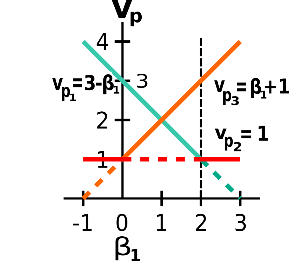
(a) Predicted coefficient($\boldsymbol{v_{p}{}}$)

(b) Predicted optimal value(POV)

(c) True optimal value(TOV)

Transition point extraction

Demirovic et al. (2020) represent optimization coefficients as parameterised linear functions. They solve the optimization problem with dynamic programming using piece-wise linear algebra and parameterised coefficients. The output of the DP solution gives the piecewise linear function POV. However this method is limited to problems with a DP solution. In addition, the DP solution requires constructing the full PWLF for every problem set. For larger problems this may result in long run times. Instead we propose a numerical approach to extract transition points. Our approach works for any arbitrary optimization problem with a linear objective.

Figure 2: Divide and conquer algorithm

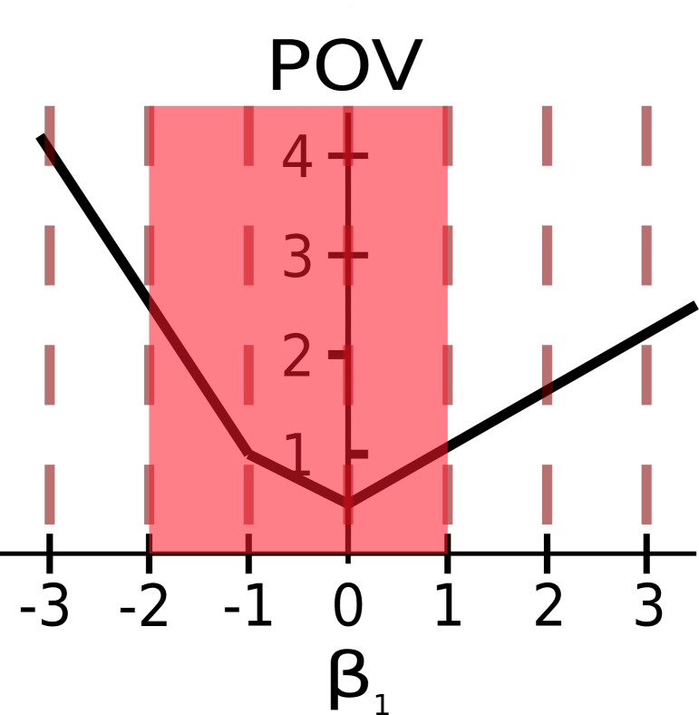
(a) Sample points with large and uniform step size. The algorithm finds a transition point in the interval [-2,1]

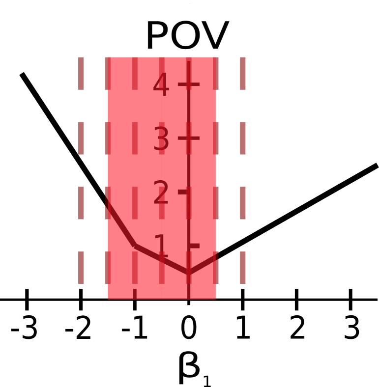
(b) The algorithm decreases the step size and narrows the transition point to the interval [-1.5,0.5]

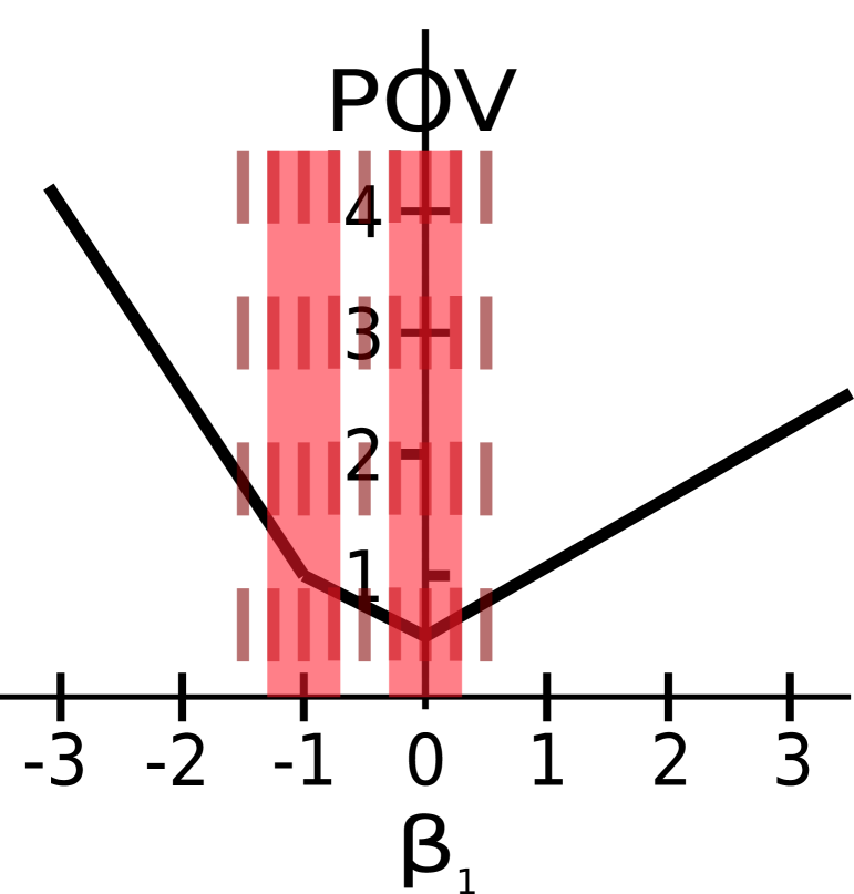
(c) With a precise step size, the algorithm identifies two transition points in the intervals [-1.25,-0.75] and [-0.25,0.25]

Divide and conquer: From corollary 1, we know that if we compare arbitrary three points of POV and they are not collinear, then there is at least one transition point between those values. When we decrease the distance between these three values, we can accurately identify the location of transition points. The simplest way to extract transition points is to sample POV with a fixed step size, and compare collinearity of consecutive three points. Clearly this brute force method can be infeasible for many problems except the easiest ones. Especially for long intervals without transition points, using a small step size is redundant. With these insights in mind we apply a divide and conquer algorithm to sample POV. First we split the search region with ten uniformly spread points, then we test collinearity of these points. If we find any points that are not collinear, we mark the intervals defined by these points as transition intervals. Finding a transition interval means that there is at least one transition point in the interval. Then we proceed to decrease the step size as: $step_{n+1}=\frac{step_{n}}{10}$ and sample the transition intervals. Finally we repeat finding transition intervals, and reducing the step size until the step size reaches a desired minimum. By starting with a large step size and iteratively reducing it, we identify long intervals without transition points with minimal processing (Fig  2(c)).

Coordinate Descent: We described a method to construct the piece-wise linear function POV and extract transition points by comparing collinearity of sample points. However we assumed single dimensional parameterised coefficients. In reality multi-variate models are widely used to predict these coefficients. We use coordinate descent to transform a multivariate linear model into a one dimensional model (Wright 2015). For a parameter vector $\boldsymbol{\beta}=[\beta_{1},...,\beta_{m}]$, coordinate descent iterates over $\boldsymbol{\beta}$. In each iteration one parameter, $\beta_{k}$, is considered as a variable, and the rest are fixed as a constant, $v_{p}{}=\beta_{k}\cdot\theta_{k}+\sum_{n\neq k}\beta_{n}\cdot\theta_{n}$. Then for each parameter we consecutively perform transition point extraction and parameter updates.

After all transition points are identified we proceed to pick the best overall transition intervals to update model parameters. This process is explained in detail in the next section.

Parameter Update

In a predict+optimize setting a dataset is a collection of multiple problem sets. Each problem set has the same constraints for the optimization problem, however their coefficients are different. We predict unknown coefficients for each problem set with the same model parameters, and the goal of the framework is to train model parameters to minimize the average regret across all problem sets. For a dataset of size $N$, and coefficient vectors $\boldsymbol{v}$, the dataset is denoted $D=\{\boldsymbol{v}^{(1)},...,\boldsymbol{v}^{N}\}$. We choose the model parameters $\boldsymbol{\beta}$ to minimize the average regret $R$.

$$\boldsymbol{\beta}\equiv\operatorname*{arg\,min}\frac{1}{N}\sum_{n=0}^{N}R(\boldsymbol{v}^{(n)},\boldsymbol{v_{p}{}}^{(n)})$$

Transition point comparison: We express the true objective value (TOV) of each problem set as a piece-wise function. The extraction method provides the transition points of each problem set. Let $T^{(i)}=\{\beta^{(i)}_{t_{1}},...\beta^{(i)}_{t_{L}}\}$ be the set of transition points of size $L$ for a problem set $i$. We construct the intervals of the piece wise function as $I^{(i)}=\{[\beta^{(i)}_{t_{l}},\beta^{(i)}_{t_{(}l+1)}],0<l<L,l\in\mathbb{Z}\}$. To find the optimal model parameters for a problem set $i$, we can simply calculate TOV for each interval and pick the best interval. As a single sample point for each interval is enough to calculate TOV, we choose the mid points of the intervals for calculations. Let $I_{mid}$ represent the set of mid points then $\beta^{(i)}_{opt}=\operatorname*{arg\,min}_{\beta\in I^{(i)}_{mid}}R(\boldsymbol{v}^{(i)},\boldsymbol{v_{p}{}}^{(i)})$. However, the optimal parameter for each problem set can be different. To find the optimal parameters over all problem sets, we compare over every interval from each problem set.

$$\beta_{opt}\equiv\operatorname*{arg\,min}_{\beta\in\bigcup\limits_{i=1}^{N}I^{(i)}_{mid}}\frac{1}{N}\sum_{n=0}^{N}R(\boldsymbol{v}^{(n)},\boldsymbol{v_{p}{}}^{(n)})$$

With coordinate descent we perform these comparisons for each parameter and update the parameters individually. Mini-batch: In our framework we use mini-batches to train the model parameters. A mini-batch represents a subset of problem sets. When using mini-batches we construct a quasi-gradient in the direction of the global minimum of that particular mini-batch. Then we update the model parameters with the quasi gradient. For a mini-batch $i$: $\beta_{new}=\beta_{old}+learning\_rate\cdot(\beta^{(i)}_{opt}-\beta_{old})$

Greedy Methods

To extract the transition points and compare them, we have to repeatedly solve an optimization problem. Many optimization problems are NP-hard, and obviously as the problem size increases it can become expensive to perform these actions. Therefore we propose a greedy method to partially extract transition points and a greedy method to compare only the best transition points.

Divide and Learn Max (DnL-MAX) : Normally we compare all intervals for all problem sets. If we assume there are $L$ intervals for each problem set $i$ and a total of $N$ problem sets, then we solve the optimization problem $N^{2}L$ times. For a full method the complexity scales both with the number of transition points and the size of the data. Instead we propose to first choose the optimal parameter for each problem set $i$ by $\beta^{(i)}_{opt}=\operatorname*{arg\,min}_{\beta\in I^{(i)}_{mid}}R(\boldsymbol{v}^{(i)},\boldsymbol{v_{p}{}}^{(i)})$, and then compare only the best parameters with the other problems sets:

$$\beta_{opt}=\operatorname*{arg\,min}_{\beta\in\bigcup\limits_{i=1}^{N}\beta^{(i)}_{opt}}\frac{1}{N}\sum_{n=0}^{N}R(\boldsymbol{v}^{(n)},\boldsymbol{v_{p}{}}^{(n)})$$

This reduces complexity by solving only $(N-1)N+LN$ optimization problems, and the number of transition points has minimal effect on the comparison complexity.

Divide and Learn Greedy (DnL-Greedy) : Our divide and conquer algorithm repeatedly compares the collinearity of POV samples. Depending on the complexity of the problem and the minimum step size for sample points, there can be many redundant transition points. We propose a greedy extraction method to stop the extraction at the first transition point $\beta_{t}$ that improves TOV over the old parameter $\beta_{old}$. We also prioritize regions around the old model parameter for transition point search. We observed that although TOV is not a convex function, the optimal model parameters are clustered in similar regions. Our motivation with this greedy method is to quickly iterate over parameters and bypass redundant sampling. Note that as we use only one transition point for each problem set, DnL-Greedy automatically includes the greedy comparison of DnL-MAX.

The greedy approaches do not guarantee finding the global minimum. However we show empirically they achieve the same performance as the full method, and reduce the run time dramatically.

Evaluation

In this section we detail our experiments. We experiment on two optimization problems: 0-1 knapsack and scheduling. We run experiments for four exact methods: DnL, DnL-MAX, DnL-Greedy, dynamic programming (DP) (Demirovic et al. 2020), two surrogate methods: SPO-Relax (Mandi et al. 2020), QPTL (Ferber et al. 2020) and one indirect method: ridge regression.

Dataset: We use the dataset from the ICON energy challenge  (Simonis et al. 2014) for both knapsack and scheduling problems. Data samples are collected from real electricity prices every 30 minutes, from 2011 November to 2013 January. Wind forecast, wind speed, Co2 intensity, temperature, load forecast and price forecast are used to predict actual energy prices. Note that predicting energy prices is challenging so even the best models have substantial prediction error. The same dataset was used in previous work on predict+optimize (Mandi et al. 2020; Demirovic et al. 2020).

In total there are 37877 data samples, each 48 data samples, representing a day, create a problem set. Therefore we can only use 789 optimization problems to train predict+optimize models. We split the data set into 70% train set, 10% validation set and 20% test set. Correspondingly we have 552, 79 and 157 optimization problems for training, validation and testing, respectively. In order to understand how models work for different distributions, we split the dataset into 5 folds. For each fold we train every model 10 times and use the iteration with the least validation regret. We report the performance of models over the mean and standard deviation of all folds.

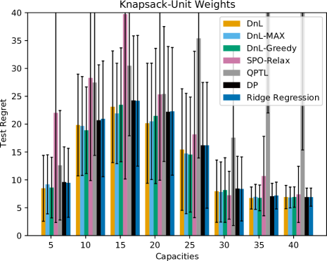
Figure 3: Unit Knapsack: showing average and one standard deviation. Note that the graph is truncated at 40 for readability.

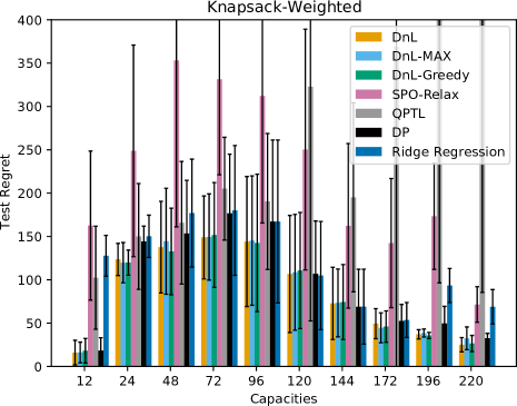
Figure 4: Weighted Knapsack: showing average and one standard deviation. SPO-Relax and QPTL are truncated at 400 for some instances for readability.

Knapsack problem: We consider a 0-1 knapsack of $n$ items, where we are given a capacity limit, $W$, item weight $\mathbf{w}=[w_{1},w_{2}...,w_{n}]$, and have to predict item values $\boldsymbol{v}=[v_{1},v_{2}...,v_{n}]$. A 0-1 solution vector $\boldsymbol{x}=\operatorname*{arg\,max}_{\boldsymbol{x}^{T}\cdot\mathbf{w}\leq W}\boldsymbol{x}^{T}\cdot\boldsymbol{v}$ decides the chosen items. We run knapsack experiments for both unit weights and varying weights. The original dataset does not have item weights, and we generate the weights synthetically. Knapsack problems with high correlation between item value and weight are considerably harder to solve than those with weak correlation (Pisinger 2005). We create exactly correlated knapsack problems by choosing weight values in $\{3,5,7\}$, and multiplying by the true energy price to generate their true value. We experiment on varying capacity limits from 5% to 90%. For unit knapsack the capacity limits range from 5-45 (10%-90%) and for weighted knapsack the capacity limits range from 12-220 (5%-90%).

Scheduling: We test on energy cost aware scheduling problems. The scheduling problems are a simplified versions of the ICON challenge (Mandi et al. 2020). There are $M$ machines and $N$ jobs. Each machine has a resource capacity $C_{m}$. Each job has a resource requirement $R_{n}$, power consumption $P_{n}$ and a duration $D_{n}$. Every job also has an earliest starting time $te_{n}$ and a latest finishing time $tl_{n}$. A job can only be run on one machine, and once a job is being processed it cannot be split. All jobs have to be finished in the 24 hour period. The goal of the scheduling is to minimize energy costs by taking energy prices into account. Energy prices are not known beforehand and have to be predicted. We consider three different loads with 3,5,3 machines and 15,20,10 machines correspondingly.

Experiments

The models are trained with Intel(R) Xeon(R) Gold 6254 CPU @ 3.10GHz processors using 8 cores with 3.10 Ghz clock speed. We use Gurobi Optimization (2020) to solve knapsack and scheduling problems. For the knapsack problems max training time is set to 4000 seconds ($\approx$ 1 hour). For scheduling problems max training time is set to 12000 seconds ($\approx$ 3.3 hours). We tune hyper-parameters via grid search for surrogate models and we use early stopping for all models  (Bishop 2006). DnL hyper-parameters are as follows: We set the mini-batch size to 32 and learning rate to $0.1$. We warmstart the model parameters with ridge regression (Pratt and Jennings 1996). The search space for transition points are bounded relative to the current value of the parameter as $[\beta-1.5\beta,\beta+1.5\beta]$. Similarly the minimum step size of models are relative to the parameter and is equal to $step_{min}=\beta/10$.

Unit knapsack: Unit knapsack (Figure 3) is a relatively simple optimization problem and there is not a large difference between regression and predict+optimize models. All variations of DnL perform identically to DP, and this suggests greedy approaches perform as well as their full counterparts. Unlike regression and exact methods, the surrogates’ performances are sensitive to the changes. SPO-Relax fails to capture the optimization problem for low capacities, while QPTL fails to capture the high capacity problem.

Weighted knapsack: The exact methods outperform surrogates for all capacities and regression for low and high capacities (Figure 4). Their advantage is more clear at the extreme capacities {12,196,220}. For capacities {72,96,196} DnL outperforms DP. At these capacities DP requires long time to build the piece-wise function and fails to finish an epoch within the time limit. In contrast for the same weights DnL-Greedy can train an epoch under 10 seconds. Similar to the unit knapsack problem SPO-Relax has higher regret for low capacities. We have observed that SPO-Relax is very sensitive to the data distribution for the weighted knapsack problem. For some folds it successfully converges at a low regret minimum. However for other folds, it converges at a higher regret than regression (Fig  5(b)). QPTL outperforms regression for low capacities but for high capacities it has the worst regret of all models. QPTL also tends to overfit the problem, though early stopping helps to identify a minimum (Fig 5(b)). These experiments show that exact methods are able to accurately search the underlying knapsack problem for all capacities, and they are more robust to changes in constraints.

Figure 5: Low capacity knapsack, test regret vs epoch plots,

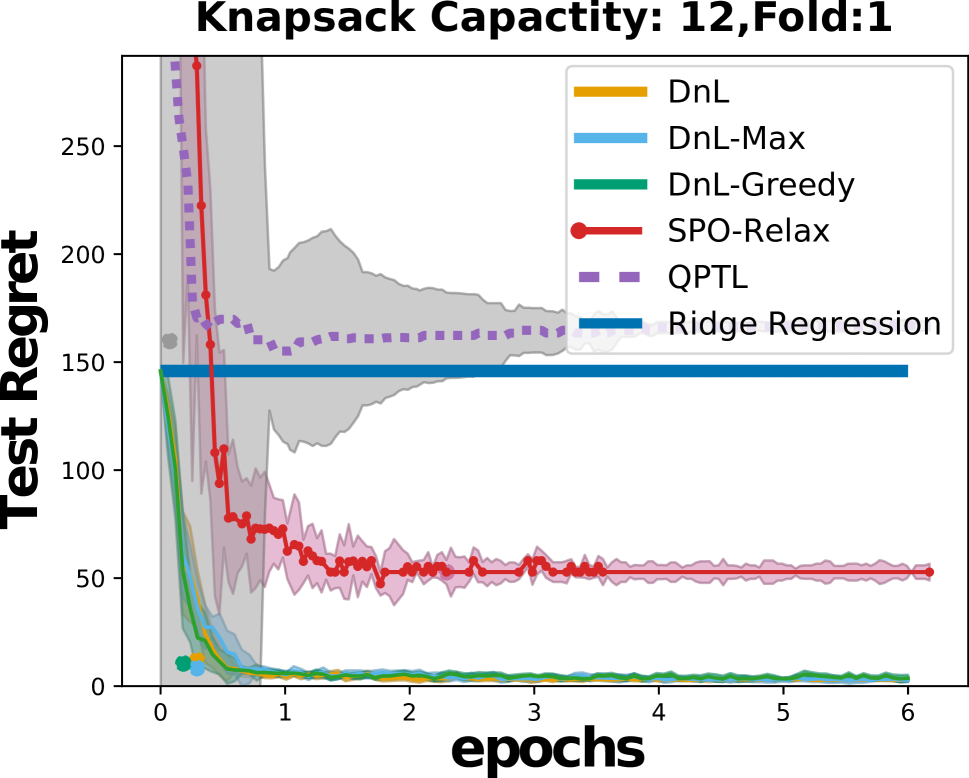
(a) weighted knapsack capacity 12,fold 1. SPO-Relax converges to low regret, QPTL overfits

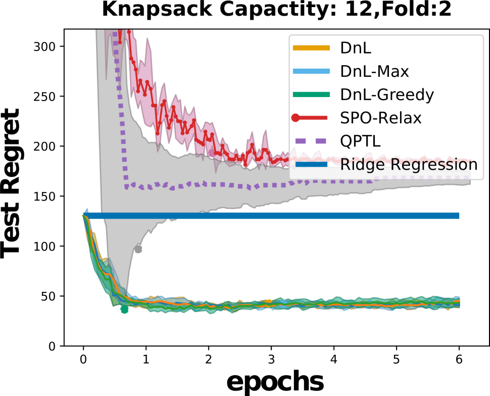
(b) weighted knapsack capacity 12,fold 2. SPO-Relax converges to high regret, QPTL overfits

Loads	1	2	3
DnL	$8382\pm{3616}$	$17168\pm{7292}$	$\boldsymbol{10347\pm{5321}}$
DnL-Greedy	$8625\pm{3829}$	$15834\pm{6259}$	$10895\pm{5626}$
SPO-Relax	$8421\pm{4144}$	$18454\pm{8302}$	$11086\pm{4752}$
QPTL	$6584\pm{2157}$	$27393\pm{12606}$	$10544\pm{5138}$
Regression	$\boldsymbol{6544\pm{4360}}$	$\boldsymbol{15672\pm{6542}}$	$10919\pm{6086}$

Table 1: ICON scheduling problems mean regret and standard deviations

Scheduling: Compared to knapsack problems scheduling problems are more complex and do not have a dynamic programming solution. As such DP method is not applicable for these problem sets and to the best of our knowledge DnL is the first exact method applicable for an arbitrary MIP problem with a linear objective. Although all frameworks have different loss models, they all converge at a similar point and we do not identify one method that clearly outperforms all the others. We believe the underlying problem for these loads, like medium capacity knapsack problems, are similar to MSE and understanding the underlying regression problem is also a successful result for predict+optimise frameworks. For Load 1, regression has the best regret, QPTL is the best predict+optimize framework, and the other three have similar regrets. Interestingly for some folds of Load 2, QPTL cannot reason over regret. We believe the solution space of these folds may resemble the high capacity knapsacks. We also observe that SPO-Relax has a higher regret than regression for Load 2. Although DnL seems to have a high regret as well, this is a result of slow training and not completing within the 4 hour limit. The greedy variation is able to complete the training and has a similar regret to the regression. For Load 3, we do not see a significant difference between the frameworks.

Scalability/runtime

Scalability is the biggest issue for exact methods. Combinatorial optimization problems are expensive to solve, and exact methods require solving multiple instances to map each problem set. Therefore we proposed greedy methods, and observed improved efficiency over the existing exact method DP. For example, DP requires more than an hour to train an epoch for knapsack capacities {72,96,196} and DnL-Greedy can complete the training of an epoch under 10 seconds. For other capacities, DP requires 200–400 seconds for an epoch, while we require 2–10 seconds. There are two reasons for this. First, the DP method has to make use of a dynamic programming solution compatible with piece wise linear algebra, which may not be the most efficient solution approach. Second, the DP constructs the entire piecewise function every time. Since the number of transition points can increase exponentially with problem size, our greedy methods can avoid computing irrelevant transition points.

Although DnL-Greedy is more scalable than the previous exact methods, it requires more processing power than surrogate methods. This difference is emphasized for larger problems. For scheduling problems (load3) DnL-Greedy requires 20 and DnL requires 30–60 minutes to train an epoch. By comparison SPO-Relax, which uses the relaxation of the optimization problem, can finish an epoch in under a minute. For a fair comparison we ran SPO-Relax for the same amount of time that we ran DnL-Greedy, but we did not observe any change in the convergence behaviour or the output regret.

Conclusion

Predict+optimize problems are challenging due to the combinatorial nature of the optimization problem. We propose a new method to train parameters using regret, rather than a surrogate or relaxation. The only previous existing method requires a DP formulation of the optimization problem, in contrast ours can be applied to any optimization problem with a linear objective. By using greedy methods to find transition points we can substantially reduce the amount of search required. Our framework outperforms regression and surrogates for weighted knapsack problems and unlike the previous DP method, is able to reason over more complex problems.

References

- Amos and Kolter (2017) Amos, B.; and Kolter, J. Z. 2017. OptNet: differentiable optimization as a layer in neural networks. In Proceedings of the 34th International Conference on Machine Learning-Volume 70, 136–145.
- Bello et al. (2016) Bello, I.; Pham, H.; Le, Q. V.; Norouzi, M.; and Bengio, S. 2016. Neural combinatorial optimization with reinforcement learning. arXiv preprint arXiv:1611.09940 .
- Bengio (1997) Bengio, Y. 1997. Using a financial training criterion rather than a prediction criterion. International Journal of Neural Systems 8(04): 433–443.
- Bishop (2006) Bishop, C. M. 2006. Pattern recognition and machine learning. springer.
- Demirovic et al. (2019a) Demirovic, E.; Bailey, J.; Chan, J.; Guns, T.; Kotagiri, R.; Leckie, C.; and Stuckey, P. J. 2019a. A Framework for Predict+Optimise with Ranking Objectives: Exhaustive Search for Learning Linear Functions for Optimisation Parameters. In Kraus, S., ed., Proceedings of the 28th International Joint Conference on Artificial Intelligence, 1078–1085. IJCAI Press. doi:https://doi.org/10.24963/ijcai.2019/151.
- Demirovic et al. (2019b) Demirovic, E.; Stuckey, P. J.; Bailey, J.; Chan, J.; Leckie, C.; Ramamohanarao, K.; and Guns, T. 2019b. Predict+ Optimise with Ranking Objectives: Exhaustively Learning Linear Functions. In IJCAI, 1078–1085.
- Demirovic et al. (2020) Demirovic, E.; Stuckey, P. J.; Guns, T.; Bailey, J.; Leckie, C.; Kotagiri, R.; and Chan, J. 2020. Dynamic Programming for Predict+Optimise. In Conitzer, V.; and Sha, F., eds., Proceedings of the Thirty-Fourth AAAI Conference on Artificial Intelligence (AAAI-20), 1441–1451. AAAI Press. doi:https://doi.org/10.1609/aaai.v34i02.5502.
- Donti, Amos, and Kolter (2017) Donti, P.; Amos, B.; and Kolter, J. Z. 2017. Task-based end-to-end model learning in stochastic optimization. In Advances in Neural Information Processing Systems, 5484–5494.
- Elmachtoub and Grigas (2017) Elmachtoub, A. N.; and Grigas, P. 2017. Smart” predict, then optimize”. arXiv preprint arXiv:1710.08005 .
- Ferber et al. (2020) Ferber, A.; Wilder, B.; Dilkina, B.; and Tambe, M. 2020. MIPaaL: Mixed Integer Program as a Layer. In AAAI, 1504–1511.
- Gurobi Optimization (2020) Gurobi Optimization, L. 2020. Gurobi Optimizer Reference Manual. URL http://www.gurobi.com.
- Horvitz and Mitchell (2010) Horvitz, E.; and Mitchell, T. 2010. From data to knowledge to action: A global enabler for the 21st century. Computing Community Consortium 1.
- Ifrim, O’Sullivan, and Simonis (2012) Ifrim, G.; O’Sullivan, B.; and Simonis, H. 2012. Properties of energy-price forecasts for scheduling. In International Conference on Principles and Practice of Constraint Programming, 957–972. Springer.
- Kao, Roy, and Yan (2009) Kao, Y.-h.; Roy, B. V.; and Yan, X. 2009. Directed regression. In Advances in Neural Information Processing Systems, 889–897.
- Li, Chen, and Koltun (2018) Li, Z.; Chen, Q.; and Koltun, V. 2018. Combinatorial optimization with graph convolutional networks and guided tree search. In Advances in Neural Information Processing Systems, 539–548.
- Lim, Shanthikumar, and Vahn (2012) Lim, A. E.; Shanthikumar, J. G.; and Vahn, G.-Y. 2012. Robust portfolio choice with learning in the framework of regret: Single-period case. Management Science 58(9): 1732–1746.
- Luo et al. (2020) Luo, C.; Qiao, B.; Chen, X.; Zhao, P.; Yao, R.; Zhang, H.; Wu, W.; Zhou, A.; and Lin, Q. 2020. Intelligent Virtual Machine Provisioning in Cloud Computing. In Bessiere, C., ed., Proceedings of the Twenty-Ninth International Joint Conference on Artificial Intelligence, IJCAI-20, 1495–1502. International Joint Conferences on Artificial Intelligence Organization. doi:10.24963/ijcai.2020/208. URL https://doi.org/10.24963/ijcai.2020/208. Main track.
- Mandi et al. (2020) Mandi, J.; Guns, T.; Demirovic, E.; and Stuckey, P. J. 2020. Smart Predict-and-Optimize for hard combinatorial optimization problems. In Conitzer, V.; and Sha, F., eds., Proceedings of the Thirty-Fourth AAAI Conference on Artificial Intelligence (AAAI-20), 1603–1610. AAAI Press. URL https://doi.org/10.1609/aaai.v34i02.5521.
- Niculae et al. (2018) Niculae, V.; Martins, A.; Blondel, M.; and Cardie, C. 2018. SparseMAP: Differentiable Sparse Structured Inference. In International Conference on Machine Learning, 3799–3808.
- Pisinger (2005) Pisinger, D. 2005. Where are the hard knapsack problems? Computers & Operations Research 32(9): 2271–2284.
- Pogančić et al. (2020) Pogančić, M. V.; Paulus, A.; Musil, V.; Martius, G.; and Rolinek, M. 2020. Differentiation of Blackbox Combinatorial Solvers. In International Conference on Learning Representations. URL https://openreview.net/forum?id=BkevoJSYPB.
- Pratt and Jennings (1996) Pratt, L.; and Jennings, B. 1996. A survey of connectionist network reuse through transfer. In Learning to learn, 19–43. Springer.
- Simonis et al. (2014) Simonis, H.; O’Sullivan, B.; Mehta, D.; Hurley, B.; and De Cauwer, M. 2014. Energy-Cost Aware Scheduling/Forecasting Competition. URL http://www.csplib.org/Problems/prob059/.
- Thapper and Živnỳ (2018) Thapper, J.; and Živnỳ, S. 2018. The limits of SDP relaxations for general-valued CSPs. ACM Transactions on Computation Theory (TOCT) 10(3): 1–22.
- Wilder, Dilkina, and Tambe (2019) Wilder, B.; Dilkina, B.; and Tambe, M. 2019. Melding the data-decisions pipeline: Decision-focused learning for combinatorial optimization. In Proceedings of the AAAI Conference on Artificial Intelligence, volume 33, 1658–1665.
- Wright (2015) Wright, S. J. 2015. Coordinate descent algorithms. Mathematical Programming 151(1): 3–34.