Understanding Guided Image Captioning Performance across Domains

Abstract

Image captioning models generally lack the capability to take into account user interest, and usually default to global descriptions that try to balance readability, informativeness, and information overload. We present a Transformer-based model with the ability to produce captions focused on specific objects, concepts or actions in an image by providing them as guiding text to the model. Further, we evaluate the quality of these guided captions when trained on Conceptual Captions which contain 3.3M image-level captions compared to Visual Genome which contain 3.6M object-level captions. Counter-intuitively, we find that guided captions produced by the model trained on Conceptual Captions generalize better on out-of-domain data. Our human-evaluation results indicate that attempting in-the-wild guided image captioning requires access to large, unrestricted-domain training datasets, and that increased style diversity (even without increasing the number of unique tokens) is a key factor for improved performance.

1 Introduction

Describing the content of an image using natural language is generically referred to as image captioning, but there are a variety of ways in which this can be achieved: by focusing on the most salient aspects of an image, as in MSCOCO Lin et al. (2014) or Conceptual Captions Sharma et al. (2018); on most of the groundable concepts in an image, as in Image Paragraphs Krause et al. (2017) or Localized Narratives Pont-Tuset et al. (2020); or on a predefined set of objects, as in dense captioning Johnson et al. (2016). These various approaches acknowledge that a typical real-world image may contain a varying number of objects/concepts/actions that may be of interest to the caption consumer, and therefore the optimal description depends on the degree to which the caption covers what the user is interested in at any given moment.

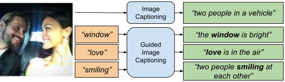
Figure 1: An illustration comparing the difference between an image captioning model and a guided image captioning model. The guided image captioning model generates captions that focus on a specific object, concept or action of the image, provided to the model as free-form guiding text.

However, the vast majority of captioning solutions lack the ability to take into account user interest, and usually default to global descriptions. Such a description might say, for example “people attending a birthday party”, which may not satisfy a user interested in a description of “the cake”. In this paper, we capture user interest via the guiding text, a free-form text input that is assumed to be related to some concept(s) in the image; and we consider the Guided Image Captioning task, where the guiding text is provided to the model as an additional input to control the concepts that an image caption should focus on. This could, for instance, enable accessibility tools for visually-impaired users, who can select a guiding text produced from an upstream object/label detector to receive a guided description of their surroundings. Note that guiding texts are not limited to a set of boxable objects, but include concepts (e.g. “vacation”, “love”) and actions (e.g. “swimming”).

A key question we ask in this work is what kind of training data can lead to models that work better in a real-world setting. Ideally, the training data should contain multiple captions for a given image, each associated with a different guiding text. The Visual Genome dataset Krishna et al. (2017a) provides exactly that, with a total of 3.6M object-level captions created through human annotation. In contrast, the Conceptual Captions Sharma et al. (2018) contains only image-level captions created through an automatic pipeline obtaining images and captions from the internet. We perform human evaluations that measure caption informativeness, correctness and fluency to test our approach in a real-world setting. Interestingly, while the Conceptual Captions dataset contains a similar number of captions (3.3M), and has a lower number of unique tokens than Visual Genome, models trained on this dataset generalize better on out-of-domain data in human evaluations.

The key contributions of this paper are summarized as follows:

• Given the popularity of Transformer Vaswani et al. (2017) models for generative tasks in NLP, we use a multimodal Transformer model as a vehicle to study characteristics of the guided image captioning task. In particular, we investigate the underlying characteristics of image captioning datasets required to produce higher quality guided captions. Our results suggest that the key to solving in-the-wild guided image captioning may not be laborious human annotations, Visual Genome–style, but rather access to noisy, unrestricted-domain training datasets with high style diversity.

• We open-source the set of test images and guiding text pairs used for our human evaluation experiments in order to encourage future work in this direction and facilitate direct comparisons with our results.

2 Related Work

The task of image captioning has received considerable interest over the past decade (Chen and Zitnick, 2015; Kiros et al., 2014; Zhu et al., 2018; Donahue et al., 2015; Mao et al., 2015; Karpathy and Li, 2015; Vinyals et al., 2015a). Template-based methods (Kulkarni et al., 2013; Elliott and de Vries, 2015; Devlin et al., 2015) provide image grounding, but lack the ability to produce diverse captions, while early encoder-decoder methods (Donahue et al., 2015; Vinyals et al., 2015b; Karpathy and Li, 2015; Zheng et al., 2019; Wu et al., 2015; Sharma et al., 2018) produce diverse captions, but lack image grounding. Contemporary encoder-decoder methods (Lu et al., 2018; Cornia et al., 2019; Anderson et al., 2017; You et al., 2016; Chen et al., 2020; Mun et al., 2017; Xu et al., 2015; Fang et al., 2015), including the method proposed in this work, can generate diverse captions with image grounding.

Most similar to our work,  Zheng et al. (2019) propose the use of a guiding object and produces a caption by using a forward and backward LSTM to separately generate the caption text before and after the guiding object. In contrast, our approach involves a multi-modal Transformer model that uses layers of self-attention and cross-attention to better ground the target caption using early-fused representations for the image and the guiding text, which in our work is not limited to boxable objects.

3 Method

Given an image $\bm{I}$ and guiding text $\bm{T}=\{t_{1},...,t_{L_{T}}\}$ with $L_{T}$ tokens, the goal of Guided Image Captioning is to generate an image description $\bm{y}=\{y_{1},...,y_{L_{y}}\}$ with $L_{y}$ tokens, such that $\bm{y}$ focuses on the concepts provided in $\bm{T}$. Note that we do not necessitate our model to include the tokens of $\bm{T}$ inside $\bm{y}$, yet we find that our trained model produces $\bm{T}$ inside $\bm{y}$ a majority of the time. Interestingly, in some cases where $\bm{T}$ is absent from $\bm{y}$, we find that $\bm{T}$ is paraphrased in $\bm{y}$. See Figure 5 for examples. Both $t_{i}$ and $y_{i}$ are tokens in the shared model vocabulary.

We employ a Transformer (Vaswani et al., 2017) based sequence to sequence model, with parameters $\bm{\theta}$ where $\bm{I}$ and $\bm{T}$ are inputs to the encoder and $\bm{y}$ is the decoder output. We use a dataset with $(\bm{I},\bm{T},\bm{y})$ tuples to search for the optimal model parameters $\bm{\theta^{*}}$ by maximizing the likelihood of the correct caption given below.

$$\bm{\theta^{*}}=\operatorname*{argmax}_{\bm{\theta}}\sum_{(\bm{I},\bm{T},\bm{y})}\log{p(\bm{y}|\bm{I},\bm{T};\bm{\theta})}$$ (1)

In our model, the encoder input sequence comprises of image features followed by sub-token embeddings for the guiding text. We use a joint encoder for both image and guiding text to transform the image features in the context of the guiding text concepts and vice versa, such that the decoder input is conditioned on the joint text-image representation.

We represent the input image as a sequence of global and regional features, G and R, respectively. Following Changpinyo et al. (2019), we use Graph-Regularized Image Semantic Embedding (GraphRISE) as the global image features G. These 64-dimensional features, trained to discriminate O(40M) ultra-fine-grained semantic labels, have been shown to outperform other state of the art image embeddings Juan et al. (2019).

For regional features, we first compute bounding boxes using a Region Proposal Network (RPN). Following Anderson et al. (2018), we reimplement the Faster R-CNN (FRCNN) model trained to predict selected labels (1,600 objects and 400 attributes) in Visual Genome Krishna et al. (2017b). This model returns $K$ bounding box regions, each with a 2048-dimensional feature vector. Changpinyo et al. (2019) observed that decoupling box proposal and featurization could improve downstream tasks. Thus, we obtain two sets of regional features – $\mbox{R}_{\textsubscript{GR}}$ and $\mbox{R}_{\textsubscript{FRCNN}}$ where the bounding box feature extractor are GraphRISE and FRCNN respectively. We experimented with using either or both of these features for the top 16 regions.

3.1 Encoder

Figure 2: Our model architecture. Thick arrows indicate a sequence, such as bounding boxes for image regions, or list of tokens in a text.

All models in the image feature extraction pipeline, are pre-trained and are not fine-tuned during our model training process. To transform them into the encoder input space, we use a trainable fully-connected network for each type of feature, denoted as $FC$ in Figure 2. The guiding text is provided to the encoder as a sequence of sub-tokens, T, which are embedded in the input space using trainable embeddings.

To summarize, the input to the Transformer encoder is a sequence of features in the following order.

G:

Global image features by Graph-RISE, 64D vector.

$\mbox{R}_{\textsubscript{GR}}$:

Sequence of 16 regional image features, 64D each, obtained by running GraphRISE on each image region.

$\mbox{R}_{\textsubscript{FRCNN}}$:

Sequence of 16 regional image features, 2048D each, obtained from FRCNN for each image region.

T:

Sequence of sub-tokens corresponding to the guiding text.

3.2 Decoder

The Transformer decoder generates the output caption sequence $\bm{y}$ conditioned on the encoder outputs. The decoder shares the same vocabulary and embeddings used for the guiding text by the encoder.

4 Data

We train our models on two datasets with different characteristics, we pick models according to automatic metrics computed over the validation (dev) split in each dataset. Human evaluations were conducted on a separate test set which is out-of-domain for both training datasets. The sub-token vocabulary size is set to 4000 for both datasets, but a comparison of the number of unique tokens is reported in Table 1.

4.1 Training and Validation (Dev) data

Visual Genome (VG).

Visual Genome Krishna et al. (2017b) contains dense annotations for each image, including a list of human-annotated objects and region captions (descriptions of image regions localized by a bounding box). We take all region captions and their first associated object to form $\langle\mbox{guiding text},\mbox{caption}\rangle$ pairs for each image. On average, each image has 34 such pairs, providing 3.6M $\langle\mbox{image},\mbox{guiding text},\mbox{caption}\rangle$ tuples for 107,180 images. We randomly sample 96,450 and 10,730 images for the training and validation (dev) sets respectively.

Conceptual Captions (CC).

Conceptual Captions Sharma et al. (2018) contains 3.3 million training, 15K validation image/caption pairs collected from the internet. Captions in this dataset are obtained from the alt-text of the images, and are diverse in their writing styles, however no paired object annotations are available for these captions. Instead, we use the Google Cloud Natural Language API to extract the text span considered to be the most salient entity in a caption, and treat it as the guiding text for the corresponding caption, yielding one $\langle\mbox{guiding text},\mbox{caption}\rangle$ pair per image.

	CC	VG
# of images	3.3M	107K
# of $\langle\mbox{image},\mbox{guiding text},\mbox{caption}\rangle$	3.3M	3.6M
# of unique guiding texts	43.2K	75.4K
# of unique tokens	42.6K	69.5K

Table 1: Statistics on the two datasets: Conceptual Captions (CC), Visual Genome (VG).

Length of guiding text	1	2	$\geq$ 3
CC	80.5%	16.3%	3.4%
VG	91.1%	8.3%	0.6%

Table 2: Length (in number of tokens) distribution of guiding texts in the two datasets.

Test T	unique guiding texts			unique tokens
source	cnt	$\in$ CC	$\in$ VG	cnt	$\in$ CC	$\in$ VG
GCP	889	67%	62%	929	90%	88%
FRCNN	421	98%	100%	421	99%	100%

Table 3: Percentage of unique (tokens in) test guiding texts that have been seen at training time for Conceptual Captions (CC) and Visual Genome (VG).

Comparisons of the two datasets.

As shown in Table 2, the guiding texts are dominated by single-word expressions with a minority of multi-word expressions (19.5% for CC; 8.9% for VG). Both datasets have a similar number of $\langle\mbox{image},\mbox{guiding text},\mbox{caption}\rangle$ tuples. While VG has significantly fewer images, it has a much higher number of unique guiding texts and its number of unique tokens in guiding texts and captions combined is larger than that of CC (Table 1).

Which type of dataset is more suitable to train a guided image captioning model? The VG dataset contains human-quality guiding texts and corresponding captions, even for small regions in the image and also has a higher number of unique tokens. In contrast, the CC dataset contains noisy guiding texts automatically extracted from captions, which potentially focus only on the most salient concept in the image. However, it has more image diversity, and its captions reflect more diverse styles as a result of a much larger set of authors. Although the model trained with CC is exposed to only one $\langle\mbox{guiding text},\mbox{caption}\rangle$ pair per image compared to VG which has on average 34 $\langle\mbox{guiding text},\mbox{caption}\rangle$ pairs per image, it may still learn to correctly generate descriptions for different concepts in an image, because it has been exposed to different ways of describing such images.

		Automatic Metrics on Dev Set				Human Score on T2
Train/Dev	Model	CIDEr	SPICE	ROUGE-L	METEOR	GCP	FRCNN
CC	Set output to T	0.580	0.301	0.204	0.087	-	-
	T	1.079	0.250	0.301	0.147	-	-
	G	0.808	0.171	0.242	0.117	-	-
	T + G	1.683	0.337	0.383	0.204	-	-
	T + G + $\mbox{R}_{\textsubscript{FRCNN}}$	1.685	0.337	0.383	0.205	-	-
	T + G + $\mbox{R}_{\textsubscript{GR}}$	1.718	0.341	0.387	0.208	0.73	0.75
	T + G + $\mbox{R}_{\textsubscript{GR}}$ + $\mbox{R}_{\textsubscript{FRCNN}}$	1.695	0.339	0.387	0.206	0.69	0.75
VG	Set output to T	1.108	0.372	0.277	0.119	-	-
	T	1.589	0.344	0.336	0.186	-	-
	G	0.406	0.109	0.183	0.079	-	-
	T + G	1.606	0.355	0.340	0.190	-	-
	T + G + $\mbox{R}_{\textsubscript{FRCNN}}$	1.758	0.376	0.357	0.204	-	-
	T + G + $\mbox{R}_{\textsubscript{GR}}$	1.744	0.373	0.354	0.202	0.62	0.79
	T + G + $\mbox{R}_{\textsubscript{GR}}$ + $\mbox{R}_{\textsubscript{FRCNN}}$	1.775	0.377	0.362	0.206	0.66	0.84

Table 4: Automatic metrics and Human evaluation results for model variations trained on Conceptual Captions (CC) and Visual Genome (VG). Each model corresponds to a different set of inputs to the Transformer encoder. The first row for each dataset is a “no-op model” that simply copies the guiding text to output to compute baseline metrics. Human evaluations are conducted with two sets of guiding texts obtained for the test images – from Google Cloud API (GCP) and an FRCNN model. In all but one case, the model with higher CIDEr score (note that CIDEr score is only comparable within the same dataset) is also the one receiving better average human ratings.

4.2 Test data

Images

For human evaluation, we use the T2 test set (i.e. 1000 images sampled from the Open Images Dataset Kuznetsova et al. (2020) for the Conceptual Captions challenge) and these images are out-of-domain for both training datasets.

Guiding Texts

The T2 dataset does not provide any groundtruth annotations. However, we want to evaluate models on multiple guiding texts for each image, in order to test their ability to generate different captions. To this end, we compile a list of up to 6 guiding texts for each T2 test image as described below, which we release for reproducibility. This is intended to simulate the scenario where a visually-impaired user is given a set of candidate guiding texts generated by an upstream model, and picks the one they are interested in learning more about. The guiding text chosen by the user is then provided as input to our model. Specifically, we use the following two approaches, and consider up to 3 test guiding texts per image from each.

GCP

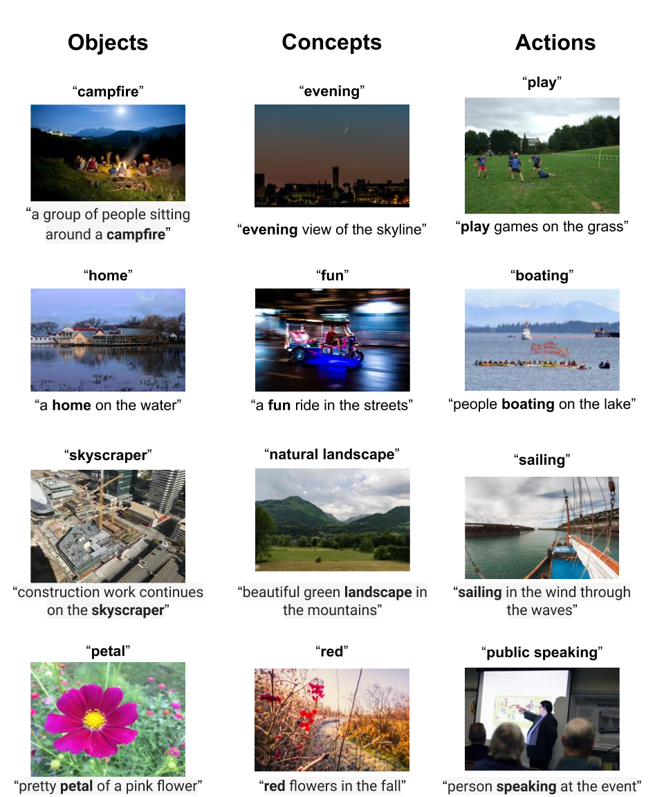
Figure 4: Sample outputs for T2 set using the model trained on Conceptual Captions with GCP labels extracted as guiding text and evaluated on GCP labels. The first, second and third columns display samples with object-based, concept-based and action-based guiding text respectively.

Three GCP labels are obtained using the image labelling API from Google Cloud by sorting labels by confidence scores and randomly sampling one from each tertile. The GCP labels generated for the T2 set can be an object (i.e. a box can be drawn around it to show its location in the image), a concept (a box cannot be drawn around it) or an action (i.e. a verb). Through manual inspection we find that 53.43% are objects (e.g. “airplane”, “coin”, “desk”), 41.73% are non-object concepts (e.g., “love”, “adventure”, “software engineering”) and 4.84% are actions. Figure 4 displays example GCP labels as well as sample outputs of each type of guiding text.

FRCNN

The other three guiding texts are FRCNN objects obtained from the faster R-CNN model described in Section 3 by also sorting the objects based on confidence and randomly sampling one from each tertile. Since the model is trained on VG annotations, and its region proposal is used in our image representations, this simulates a much more in-domain type of guiding texts. As expected, all of the FRCNN-based guiding texts have appeared in the training guiding texts of VG (Table 3).

Overall, GCP-based guiding texts have a significantly lower overlap with our training data (for both CC and VG), as compared to FRCNN-based guiding texts. We find that 67% and 62% of the GCP labels are seen at training time for CC and VG respectively, while 98% and 100% of the FRCNN objects are seen at training time for CC and VG respectively. We consider our analysis with FRCNN objects as an in-domain type of guiding text and GCP labels as an out-of-domain type of guiding text.

This set of images, together with the guiding text used in our experiments, is made available in order to encourage future work in this direction and facilitate direct comparisons with our work.

5 Experiments

5.1 Model Implementation Details

Our Transformer contains a stack of 6 layers each for both the encoder and decoder, with 8 attention heads. All models were optimized with a learning rate of 0.128 using stochastic gradient descent (SGD) and a decay rate of 0.95. Decoding was performed using beam search with a beam width of 5. The T + G + $\mbox{R}_{\textsubscript{GR}}$ + $\mbox{R}_{\textsubscript{FRCNN}}$ model has a total of 48.6M trainable parameters, while the T + G + $\mbox{R}_{\textsubscript{GR}}$ model has 47.3M trainable parameters. We use a batch size of 4096 on a 32-core Google Cloud TPU. All models are trained to optimize the CIDEr performance on the validation set, which typically takes approximately 2 million and 4 million steps for Visual Genome and Conceptual Captions models, respectively. With this setup, convergence for Visual Genome models typically takes 3 days, while Conceptual Captions takes 6 days.

We start from the initial hyperparameters from Changpinyo et al. (2019), and perform an additional hyperparameter search for the learning rate and decay rate for SGD. The values used for the learning rate are {0.0016, 0.008, 0.016, 0.048, 0.096, 0.128, 0.16}, while for the decay rate are {0.90, 0.95}. We choose the learning rate and decay rate with the highest validation CIDEr score (i.e. 0.128 learning rate and 0.95 decay rate), and use the same hyperparameters for all models.

5.2 Automatic evaluation results

We start by examining model performances via automatic evaluation metrics. The CC-trained model is evaluated on the CC validation set, and the VG-trained model is evaluated on the VG validation set. Note that the automatic evaluation metric results are only comparable within each dataset.

As shown in Table 4, providing guiding texts as additional input to the model outperforms the model with image-only input (model T + G vs model G) for both datasets. This confirms the expectation that with either dataset, the model does learn to produce captions based on the guiding texts. Model T + G also outperforms a trivial baseline method where the prediction reproduces the guiding text verbatim (“Set output to T”), and a stronger baseline, where only the guiding text is given as input to the model (Model T + G vs model T), confirming that the model does learn from the global image features as well. Note that the VG-trained model achieves much higher CIDEr scores with the T baseline, indicating that the dataset contains more image-independent, formulaic expressions (e.g. “white clouds in blue sky”). Also, note that the a VG image has several (guiding text, image, caption) triples; with the guiding text removed, the G model is trained on multiple (image, caption) pairs, i.e. multiple targets for the same input, potentially causing the performance to be lower.

The most important result here is that, for both datasets, the models that use both image features and guiding text achieve significantly higher scores than the T baseline, indicating that these models are capable of learning additional, image-specific information about the guiding text. Note that we observe a bigger improvement by adding image features to model T when training on the CC data (1.079 $\to$ 1.718 = +0.639 CIDEr), compared to the VG dataset (1.589 $\to$ 1.775 = +0.186 CIDEr).

Table 4 also shows the effects of different visual features. $\mbox{R}_{\textsubscript{FRCNN}}$ has a stronger positive effect on the Visual Genome dataset, most likely because the model that produces these features is trained on Visual Genome data. The top two performing models for each dataset were sent for human evaluation, and we found that the human evaluation results correlated with the automatic metrics.

See Figure 3 for qualitative examples of models trained with different datasets. From Figure 3, we observe that although CC target captions are generally longer, our model naturally generates shorter captions even though we do not restrict the number of output tokens in the output caption.

5.3 Human Evaluations

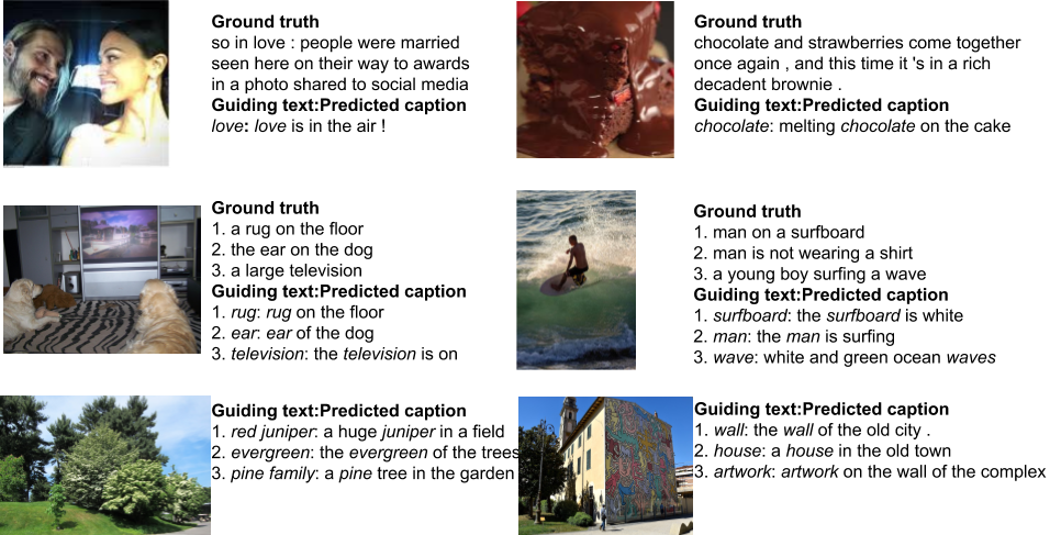
Figure 3: Example qualitative results for CC images using model T + G + $\mbox{R}_{\textsubscript{GR}}$ trained on CC (first row), VG images using model T + G + $\mbox{R}_{\textsubscript{GR}}$ + $\mbox{R}_{\textsubscript{FRCNN}}$ trained on VG (second row), T2 images using model T + G + $\mbox{R}_{\textsubscript{GR}}$ trained on CC where guiding text is extracted using the Google Cloud Natural Language API (third row).

For human evaluations over T2 images, each predicted caption is rated by three raters. Our rater pool consisted a total of 12 raters. Raters are shown an image, a guiding text, along with a generated image caption. If the guiding text is judged to be present in the image, the rater is asked to rate the predicted caption across the following three dimensions; their choice will be converted to a score between 0 and 1 according to the following scheme:

Informativeness

: For someone who cannot see the image, does the caption provide additional information about the object?

• No useful info provided [0.0]

• Some useful info provided [0.5]

• Key info provided [1.0]

Correctness

: Is the additional information correct?

• Incorrect [0.0]

• Partially correct [0.5]

• Correct [1.0]

Fluency

: Does the caption read fluently?

• Not fluent. [0.0]

• Fluent [1.0]

	Human score on T2				Diversity		T $\in$ cap?
$\mathcal{D}$	$H_{I}$	$H_{C}$	$H_{F}$	Avg	Div-1	Div-2	= %	$\approx$ %
Test $T$ = GCP
CC	0.63	0.68	0.88	0.73	0.74	0.92	83.9	12.5
VG	0.57	0.61	0.79	0.66	0.78	0.94	55.7	15.0
MX	0.70	0.68	0.88	0.75	0.78	0.94	86.7	11.5
Test $T$ = FRCNN
CC	0.65	0.67	0.94	0.75	0.76	0.94	98.3	0.2
VG	0.75	0.80	0.96	0.84	0.74	0.92	99.8	0.2
MX	0.74	0.72	0.95	0.80	0.78	0.95	99.5	0.1

Table 5: Human evaluation results on T2 with the best models from each dataset ($\mathcal{D}$): Conceptual Captions (CC), Visual Genome (VG) and mixing both (MX). Each instance was replicated three times and rated against informativeness ($H_{I}$), correctness ($H_{C}$) and fluency ($H_{F}$); we report average score across these three scales ranging from 0 to 1. We report the n-gram diversity for uni-gram (Div-1) and bi-gram (Div-2). Last two columns report the percentage cases where the input guiding text T appears verbatim (=) or paraphrased ($\approx$) in the output caption.

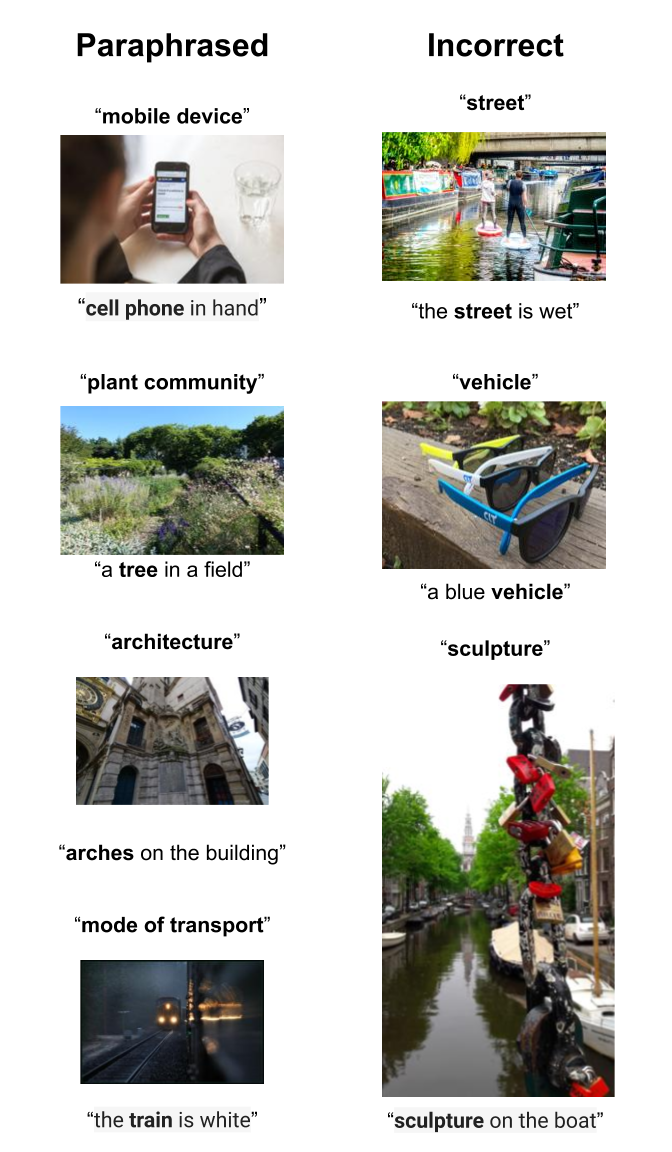
Figure 5: Examples of captions that paraphrased the guiding text (first column) and examples of captions produced from guiding text that are absent from the image (second column). Sample outputs are obtained on the T2 set using the model trained on Visual Genome with its own annotations as guiding text and evaluated on GCP labels.

Table 5 reports the average scores per dimension ranging from 0 to 1. We observe that the VG-trained model performs significantly worse than the CC-trained model for out-of-domain GCP-based guiding texts. One may hypothesize that the VG-trained model performs worse, because it contains fewer images than CC. However, from Table 5 we also observe that the VG-trained model performs better than the CC-trained model for in-domain FRCNN-based guiding texts. This suggests that the VG-trained model has a harder time adapting to the out-of-domain guiding texts, rather than the out-of-domain images. But recall from Section 4.2, the GCP-based guiding texts have similar levels of overlap with these two datasets, so why does the VG-trained model perform worse? One potential reason could lie in the distribution of the guiding texts: entropy of guiding texts is significantly lower for VG with $H(T)$ = 9.7 bits, vs $H(T)$= 10.6 bits for CC, even though VG has a higher number of unique guiding texts and a higher number of unique tokens. We posit that variety in the training data is important when adapting to out-of-domain guiding texts.

5.4 Caption Diversity

Recall that we produce three captions for each image given three different guiding texts. In Table 5, we report the n-gram diversity Deshpande et al. (2019) for unigrams (Div-1) and bigrams (Div-2) by computing the number of distinct n-grams from the three predicted captions divided by the total number of n-grams from these three captions. Our Div-1 ranges 0.74 - 0.78, and Div-2 ranges from 0.92 to 0.95, showing that our model generates diverse captions for the same image when prompted by different guiding texts.

5.5 Guiding Text paraphrasing in Caption

Table 5 also reports the percent of instances where the guiding text is present verbatim or paraphrased in the predicted caption, based on manual inspection. Interestingly, we observe cases where paraphrasing the guiding text leads to a better caption. For example: “mobile device” to “cell phone in hand”, “red juniper” to “a huge juniper in a field”, and “pine family” to “a pine tree in the garden” (Figure 3).

Figure 5 displays sample outputs with captions that paraphrase the guiding text and sample outputs that use incorrectly labelled guiding text (i.e., the guiding text is not present in the image).

$\mathcal{D}$	$H_{I}$	$H_{C}$	$H_{F}$	Avg	Div-1	Div-2
$\mbox{CC}_{\textsubscript{GCP}}$	0.71	0.76	0.96	0.81	0.77	0.94
$\mbox{VG}_{\textsubscript{GCP}}$	0.55	0.63	0.92	0.70	0.77	0.94
$\mbox{MX}_{\textsubscript{GCP}}$	0.69	0.74	0.95	0.79	0.75	0.92
$\mbox{CC}_{\textsubscript{FRCNN}}$	0.73	0.69	0.96	0.79	0.76	0.94
$\mbox{VG}_{\textsubscript{FRCNN}}$	0.81	0.82	0.99	0.87	0.78	0.95
$\mbox{MX}_{\textsubscript{FRCNN}}$	0.77	0.75	0.98	0.83	0.78	0.95

Table 6: Human evaluation results with the best models from each dataset. These results were trained with guiding texts extracted using GCP or FRCNN.

5.6 Train with an Object or Label Detector

For the results we report in Section 5.3, the training guiding texts are either extracted from the ground truth captions (CC) or from human annotations (VG). If we already have access to the upstream model that provides candidate guiding texts, we can potentially take advantage of this at training time to create a more streamlined model. For this experiment, we run the FRCNN object and GCP label detector on our training images to obtain training guiding texts. To ensure that the ground truth caption is relevant to the guiding text constructed this way, we only retain the training tuples in which the guiding text is present in the groundtruth caption, using a text-match filter. For CC, this filter reduces the training tuples from 3.3M to 1.1M when using the FRCNN object detector, and from 3.3M to 2.4M when using the GCP label detector. For VG, the filter reduces the training tuples from 3.6M to 2.4M when using the FRCNN object detector, and from 3.6M to 1.2M when using the GCP label detector. Taking the models with the highest CIDEr score for each dataset and guiding text, we perform another human evaluation and report the scores in Table 6. We note that the average scores obtained are all higher than their counterparts in Figure 5, showing that training with a guiding text distribution that matches the inference-time guiding text distribution generally leads to better results, e.g., about +8 points across all three dimensions for GCP guiding texts under CC.

6 Conclusion

In this work, we compare Conceptual Captions and Visual Genome to analyze and determine which type of training set performs better Guided Image Captioning on out-of-domain data. We show that although Visual Genome has human-annotated object-level captions and a higher number of unique tokens, training on the Conceptual Captions dataset with web-collected image-level captions that have a high diversity of writing styles and are image-dependent (unlike Visual Genome which has many image-independent target captions) produces better guided captions on out-of-domain data. Our results suggest that creating a good guided image captioning training set does not require laborious human annotations and that building these datasets by automatically scraping the internet which has the side effect of being more easily scaled-up can lead to better performance.

Appendix A Examples of Human Evaluation Form

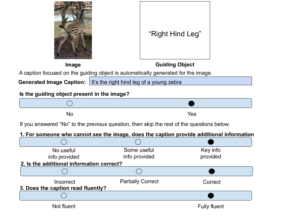
Figure 6: Human evaluation form for raters to rate predicted captions.

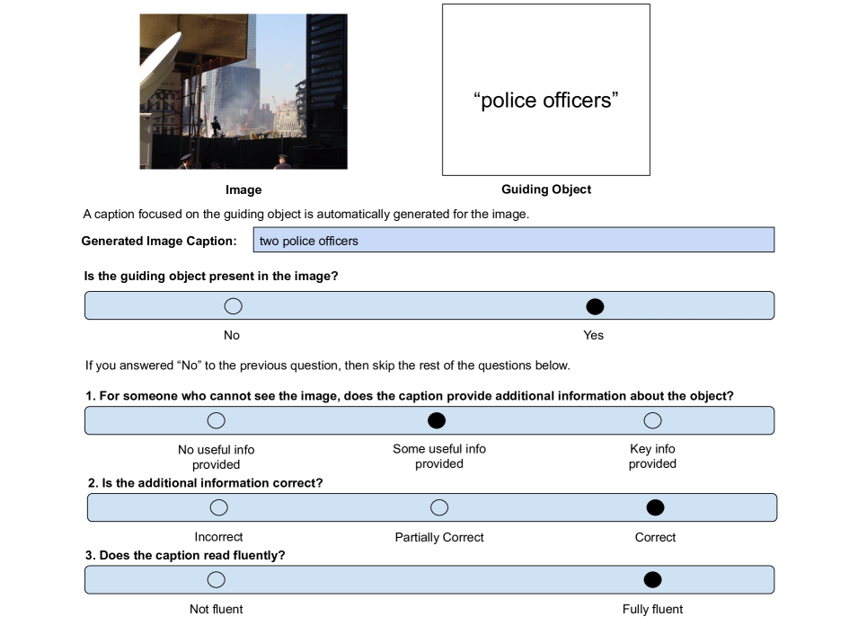
Figure 7: Example human evaluation form with caption that should receive partial score for informativeness.

References

- Anderson et al. (2017) Peter Anderson, Basura Fernando, Mark Johnson, and Stephen Gould. 2017. Guided open vocabulary image captioning with constrained beam search. In Proceedings of the 2017 Conference on Empirical Methods in Natural Language Processing, pages 936–945.
- Anderson et al. (2018) Peter Anderson, Xiaodong He, Chris Buehler, Damien Teney, Mark Johnson, Stephen Gould, and Lei Zhang. 2018. Bottom-up and top-down attention for image captioning and visual question answering. In Proceedings of CVPR.
- Changpinyo et al. (2019) Soravit Changpinyo, Bo Pang, Piyush Sharma, and Radu Soricut. 2019. Decoupled box proposal and featurization with ultrafine-grained semantic labels improve image captioning and visual question answering. In EMNLP-IJCNLP.
- Chen et al. (2020) Shizhe Chen, Qin Jin, Peng Wang, and Qi Wu. 2020. Say as you wish: Fine-grained control of image caption generation with abstract scene graphs. In Proceedings of the IEEE/CVF Conference on Computer Vision and Pattern Recognition, pages 9962–9971.
- Chen and Zitnick (2015) Xinlei Chen and Lawrence C Zitnick. 2015. Mind’s eye: A recurrent visual representation for image caption generation. In Proceedings of the IEEE conference on computer vision and pattern recognition, pages 2422–2431.
- Cornia et al. (2019) Marcella Cornia, Lorenzo Baraldi, and Rita Cucchiara. 2019. Show, control and tell: a framework for generating controllable and grounded captions. In Proceedings of the IEEE Conference on Computer Vision and Pattern Recognition, pages 8307–8316.
- Deshpande et al. (2019) Aditya Deshpande, Jyoti Aneja, Liwei Wang, Alexander G Schwing, and David Forsyth. 2019. Fast, diverse and accurate image captioning guided by part-of-speech. In Proceedings of the IEEE Conference on Computer Vision and Pattern Recognition, pages 10695–10704.
- Devlin et al. (2015) Jacob Devlin, Hao Cheng, Hao Fang, Saurabh Gupta, Li Deng, Xiaodong He, Geoffrey Zweig, and Margaret Mitchell. 2015. Language models for image captioning: The quirks and what works. In Proceedings of the 53rd Annual Meeting of the Association for Computational Linguistics and the 7th International Joint Conference on Natural Language Processing (Volume 2: Short Papers), pages 100–105.
- Donahue et al. (2015) Jeffrey Donahue, Lisa Anne Hendricks, Sergio Guadarrama, Marcus Rohrbach, Subhashini Venugopalan, Kate Saenko, and Trevor Darrell. 2015. Long-term recurrent convolutional networks for visual recognition and description. In Proceedings of the IEEE conference on computer vision and pattern recognition, pages 2625–2634.
- Elliott and de Vries (2015) Desmond Elliott and Arjen de Vries. 2015. Describing images using inferred visual dependency representations. In Proceedings of the 53rd Annual Meeting of the Association for Computational Linguistics and the 7th International Joint Conference on Natural Language Processing (Volume 1: Long Papers), pages 42–52.
- Fang et al. (2015) Hao Fang, Saurabh Gupta, Forrest Iandola, Rupesh K Srivastava, Li Deng, Piotr Dollár, Jianfeng Gao, Xiaodong He, Margaret Mitchell, John C Platt, et al. 2015. From captions to visual concepts and back. In Proceedings of the IEEE conference on computer vision and pattern recognition, pages 1473–1482.
- Johnson et al. (2016) Justin Johnson, Andrej Karpathy, and Li Fei-Fei. 2016. Densecap: Fully convolutional localization networks for dense captioning. In Proceedings of the IEEE conference on computer vision and pattern recognition, pages 4565–4574.
- Juan et al. (2019) Da-Cheng Juan, Chun-Ta Lu, Zhen Li, Futang Peng, Aleksei Timofeev, Yi-Ting Chen, Yaxi Gao, Tom Duerig, Andrew Tomkins, and Sujith Ravi. 2019. Graph-rise: Graph-regularized image semantic embedding. CoRR, abs/1902.10814.
- Karpathy and Li (2015) Andrej Karpathy and Fei-Fei Li. 2015. Deep visual-semantic alignments for generating image descriptions. In Proc. of IEEE Conference on Computer Vision and Pattern Recognition (CVPR).
- Kiros et al. (2014) Ryan Kiros, Ruslan Salakhutdinov, and Rich Zemel. 2014. Multimodal neural language models. In International Conference on Machine Learning, pages 595–603.
- Krause et al. (2017) Jonathan Krause, Justin Johnson, Ranjay Krishna, and Li Fei-Fei. 2017. A hierarchical approach for generating descriptive image paragraphs. In Computer Vision and Patterm Recognition (CVPR).
- Krishna et al. (2017a) Amrith Krishna, Pavan Kumar Satuluri, and Pawan Goyal. 2017a. A dataset for Sanskrit word segmentation. In Proceedings of the Joint SIGHUM Workshop on Computational Linguistics for Cultural Heritage, Social Sciences, Humanities and Literature, pages 105–114, Vancouver, Canada. Association for Computational Linguistics.
- Krishna et al. (2017b) Ranjay Krishna, Yuke Zhu, Oliver Groth, Justin Johnson, Kenji Hata, Joshua Kravitz, Stephanie Chen, Yannis Kalantidis, Li-Jia Li, David A. Shamma, Michael Bernstein, and Li Fei-Fei. 2017b. Visual Genome: Connecting language and vision using crowdsourced dense image annotations. IJCV, 123(1):32–73.
- Kulkarni et al. (2013) Girish Kulkarni, Visruth Premraj, Vicente Ordonez, Sagnik Dhar, Siming Li, Yejin Choi, Alexander C Berg, and Tamara L Berg. 2013. Babytalk: Understanding and generating simple image descriptions. IEEE Transactions on Pattern Analysis and Machine Intelligence, 35(12):2891–2903.
- Kuznetsova et al. (2020) Alina Kuznetsova, Hassan Rom, Neil Alldrin, Jasper R. R. Uijlings, Ivan Krasin, Jordi Pont-Tuset, Shahab Kamali, Stefan Popov, Matteo Malloci, Tom Duerig, and Vittorio Ferrari. 2020. The Open Images Dataset V4. IJCV.
- Lin et al. (2014) Tsung-Yi Lin, Michael Maire, Serge J. Belongie, Lubomir D. Bourdev, Ross B. Girshick, James Hays, Pietro Perona, Deva Ramanan, Piotr Dollár, and C. Lawrence Zitnick. 2014. Microsoft COCO: common objects in context. In Proceedings of ECCV.
- Lu et al. (2018) Jiasen Lu, Jianwei Yang, Dhruv Batra, and Devi Parikh. 2018. Neural baby talk. In Proceedings of CVPR.
- Mao et al. (2015) J. Mao, W. Xu, Y. Yang, J. Wang, and A. Yuille. 2015. Deep captioning with multimodal recurrent neural networks (mRNN). In Proc. Int. Conf. Learn. Representations.
- Mun et al. (2017) Jonghwan Mun, Minsu Cho, and Bohyung Han. 2017. Text-guided attention model for image captioning. In Thirty-First AAAI Conference on Artificial Intelligence.
- Pont-Tuset et al. (2020) Jordi Pont-Tuset, Jasper Uijlings, Soravit Changpinyo, Radu Soricut, and Vittorio Ferrari. 2020. Connecting vision and language with localized narratives. In ECCV.
- Sharma et al. (2018) Piyush Sharma, Nan Ding, Sebastian Goodman, and Radu Soricut. 2018. Conceptual Captions: A cleaned, hypernymed, image alt-text dataset for automatic image captioning. In Proceedings of ACL.
- Vaswani et al. (2017) Ashish Vaswani, Noam Shazeer, Niki Parmar, Jakob Uszkoreit, Llion Jones, Aidan N. Gomez, Lukasz Kaiser, and Illia Polosukhin. 2017. Attention is all you need. In Proceedings of NeurIPS.
- Vinyals et al. (2015a) Oriol Vinyals, Alexander Toshev, Samy Bengio, and Dumitru Erhan. 2015a. Show and tell: A neural image caption generator. In Proceedings of the IEEE conference on computer vision and pattern recognition, pages 3156–3164.
- Vinyals et al. (2015b) Oriol Vinyals, Alexander Toshev, Samy Bengio, and Dumitru Erhan. 2015b. Show and tell: A neural image caption generator. In Proc. of IEEE Conference on Computer Vision and Pattern Recognition (CVPR).
- Wu et al. (2015) Qi Wu, Chunhua Shen, Anton van den Hengel, Lingqiao Liu, and Anthony Dick. 2015. Image captioning with an intermediate attributes layer. arXiv preprint arXiv:1506.01144.
- Xu et al. (2015) Kelvin Xu, Jimmy Ba, Ryan Kiros, Kyunghyun Cho, Aaron Courville, Ruslan Salakhutdinov, Richard Zemel, and Yoshua Bengio. 2015. Show, attend and tell: Neural image caption generation with visual attention. In Proceedings of ICML.
- You et al. (2016) Quanzeng You, Hailin Jin, Zhaowen Wang, Chen Fang, and Jiebo Luo. 2016. Image captioning with semantic attention. In Proceedings of the IEEE Conference on Computer Vision and Pattern Recognition, pages 4651–4659.
- Zheng et al. (2019) Yue Zheng, Yali Li, and Shengjin Wang. 2019. Intention oriented image captions with guiding objects. In Proceedings of the IEEE Conference on Computer Vision and Pattern Recognition, pages 8395–8404.
- Zhou et al. (2020) Luowei Zhou, Hamid Palangi, Lei Zhang, Houdong Hu, Jason J. Corso, and Jianfeng Gao. 2020. Unified vision-language pre-training for image captioning and VQA. In AAAI.
- Zhu et al. (2018) Xinxin Zhu, Lixiang Li, Jing Liu, Haipeng Peng, and Xinxin Niu. 2018. Captioning transformer with stacked attention modules. Applied Sciences, 8(5):739.