Iterated Linear Optimization

Abstract

We introduce a fixed point iteration process built on optimization of a linear function over a compact domain. We prove the process always converges to a fixed point and explore the set of fixed points in various convex sets. In particular, we consider elliptopes and derive an algebraic characterization of their fixed points. We show that the attractive fixed points of an elliptope are exactly its vertices. Finally, we discuss how fixed point iteration can be used for rounding the solution of a semidefinite programming relaxation.

MSC: 90C25, 90C27, 15B48, 15A18

Keywords: Fixed Point Iteration, Linear Optimization, Semidefinite Programming, Elliptope.

1 Introduction

We introduce a fixed point iteration process built on optimization of a linear function over a compact domain. Given a domain $\Delta\subset\mathbb{R}^{n}$, the process generates a sequence $\{x_{0},x_{1},x_{2},\ldots\}$, $x_{i}\in\Delta$, where $x_{i+1}$ maximizes a linear function defined by $x_{i}$. The iteration is guaranteed to converge for all compact domains, as shown in Theorem 1. We focus on convex sets, both polyhedral and smooth. The fixed points of linear optimization reflect interesting geometric properties of the underlying convex set. Fixed point iteration is a common methodology in numerical analysis and optimization (see, e.g., [5, 4]). Moreover, fixed point iteration defines a discrete dynamical system ([11, 13]). There are several notions of stability for such systems, and we consider the attractive and repulsive fixed points of various sets.

We focus in particular on the set of fixed points of linear optimization in elliptopes. Elliptopes are a family of convex bodies that arise naturally in semidefinite programming (SDP) relaxations of combinatorial optimization problems (see, e.g., [12, 15, 17, 1]). A key step in using a convex relaxation for combinatorial optimization involves rounding. A solution found in the relaxed convex body must be rounded to a discrete solution that satisfies the initial combinatorial problem. For the elliptope, combinatorial solutions correspond precisely to its vertices. All points in the elliptope correspond to a positive semidefinite matrix of a certain form. In Theorem 15, we use this perspective to prove an algebraic characterization of the fixed points of iterated linear optimization in the elliptope. Furthermore, we show that the vertices of the elliptope are exactly the attractive fixed points of our iteration process, Theorem 20. Each step of fixed point iteration solves a relaxation to the closest vertex problem. By iterating the process we obtain a deterministic method for rounding the solution of an SDP relaxation.

The problem of rounding the solution of an SDP has fundamental applications in combinatorial optimization ([12, 10, 16, 3]). In a companion paper ([8]) we apply the fixed point iteration process to clustering. The approach is based on the classical SDP relaxation for $k$-way max-cut defined in [10], combined with iterated linear optimization for rounding.

2 Iterated Optimization

Let $\Delta\subset\mathbb{R}^{n}$ be a compact convex set containing the origin.

Let $T$ be the map defined by linear optimization over $\Delta$,

$$\textrm{for }x\in\mathbb{R}^{n},\,\,\,\,T(x)=\operatorname*{argmax}_{y\in\Delta}\,\,x\cdot y.$$

We consider the process of fixed point iteration with $T$. That is, we are interested in sequences $(x_{0},x_{1},\ldots)$ such that

$$x_{i+1}=T(x_{i}).$$

Note that the $\operatorname*{argmax}$ in the definition of $T$ may not be unique. In this case $T(x)$ is set valued. When we write $x_{i+1}=T(x_{i})$ we allow $x_{i+1}$ to be any element of $T(x_{i})$.

The fixed point iteration process can be seen as an iterative method to maximize $f(x)=\frac{1}{2}||x||^{2}$ over a convex domain. To see this let $g(x)=f(x_{i})+\nabla f(x_{i})\cdot(x-x_{i})$. The function $g(x)$ lower-bounds $f(x)$ and the two functions coincide at $x_{i}$. Since $\nabla f(x_{i})=x_{i}$ we see that $x_{i+1}$ maximizes $g(x)$. Therefore $f(x_{i+1})\geq g(x_{i+1})\geq g(x_{i})=f(x_{i})$. The use of a linear approximation in each step often leads to an optimization problem that can be solved efficiently using interior point methods and related techniques. Moreover, while $f(x)$ may have many global maxima, the fixed point iteration process can be used to find a maximum that is “near” an initial point (see Section  4.3).

The interpretation of fixed point iteration with $T$ as a method to maximize $f(x)=\frac{1}{2}||x||^{2}$ is related to the Frank-Wolfe method [9], although the Frank-Wolfe algorithm is normally used to minimize a convex function over a convex domain.

2.1 Convergence

We first prove that iteration with $T$ converges to a set of fixed points. While there are many general results about the convergence of fixed point iteration ([5]), these results do not apply to our setting because $T$ is neither contractive nor continuous.

Theorem 1.

Let $\{x_{i}\}$ be a sequence generated by iteration with $T$. Then $\{x_{i}\}$ has at least one limit point. If the sequence has more than one limit point the set of limit points is connected. Moreover, every limit point is a fixed point of $T$.

Proof.

Let $\{x_{i}\}$ be a sequence where $x_{0}\in\Delta$ is an arbitrary starting point and $\forall i$ $x_{i+1}=T(x_{i})$. Again, note that the map $T$ may be set valued, and we allow for any choice of $x_{i+1}\in T(x_{i})$ at each stage of the iteration.

By definition of $T$ we have

$$x_{i+1}\cdot x_{i}\geq x_{i}\cdot x_{i}.$$ (1)

Using $||x_{i+1}-x_{i}||^{2}\geq 0$ and (1) gives

$$x_{i+1}\cdot x_{i+1}\geq x_{i+1}\cdot x_{i}.$$ (2)

Let

$$a_{i}=x_{i}\cdot x_{i}=||x_{i}||^{2}.$$

Together (1) and (2) imply that $a_{i}\leq a_{i+1}$. Since the sequence $\{a_{i}\}$ is non-decreasing and bounded it converges. Let $a=\lim_{i\rightarrow\infty}a_{i}$.

Since the sequence $\{x_{i}\}$ is bounded there is a subsequence of $\{x_{i}\}$ that converges. Therefore the sequence $\{x_{i}\}$ has at least one limit point.

Using (1) we see that

$$||x_{i+1}-x_{i}||^{2} =x_{i+1}\cdot x_{i+1}+x_{i}\cdot x_{i}-2x_{i+1}\cdot x_{i},$$

$$\leq x_{i+1}\cdot x_{i+1}-x_{i}\cdot x_{i},$$

$$=a_{i+1}-a_{i}.$$

Therefore $\lim_{i\rightarrow\infty}||x_{i+1}-x_{i}||=0$. This implies the sequence $\{x_{i}\}$ has a single limit point or the set of limit points is connected (see, e.g., [2]).

Now let $x^{*}$ be a limit point of $\{x_{i}\}$. We claim any such $x^{*}$ is a fixed point.

Suppose $x^{*}$ is not a fixed point. Then there must exist $y\in\Delta$ such that $y\cdot x^{*}>x^{*}\cdot x^{*}$. Since there is a subsequence of $\{x_{i}\}$ that converges to $x^{*}$, there is an element $x_{i}$ that is sufficiently close to $x^{*}$ such that $y\cdot x_{i}>x^{*}\cdot x^{*}$. Since $x_{i+1}=T(x_{i})$,

$$x_{i+1}\cdot x_{i}\geq y\cdot x_{i}$$

and

$$x_{i+1}\cdot x_{i+1}\geq x_{i+1}\cdot x_{i}\geq y\cdot x_{i}>x^{*}\cdot x^{*}=a\geq x_{i+1}\cdot x_{i+1},$$

which is a contradiction. ∎

Note that if the set of fixed points in $\Delta$ is finite then any sequence $\{x_{i}\}$ generated by $T$ converges to a single fixed point $x^{*}$. This follows from the fact that the set of limit points is connected.

In this paper we focus on convex spaces $\Delta$. Note, however, that the above proof only uses compactness and not convexity.

3 Fixed Points

A fixed point of $\Delta$ is a point $x\in\Delta$ such that $x\in T(x)$. Geometrically, fixed points can be described in terms of normal cones.

For a point $x\in\Delta$, the normal cone of $\Delta$ at $x$ is the set

$$N(\Delta,x)=\{y\in\mathbb{R}^{n}\,|\,y\cdot x\geq y\cdot z\;\;\forall z\in\Delta\}.$$

Note that $x\in T(x)$, i.e. $x$ is a fixed point, exactly when $x\in N(\Delta,x)$.

The fixed points are distinguished boundary points of $\Delta$ that can be of significant interest.

Example 2 (Elliptope).

Figure 1 illustrates the fixed points of $T$ in the elliptope ${\cal L}_{3}$, a convex shape that arises in the SDP relaxation of max-cut and various other combinatorial optimization problems. In this $3$-dimensional example the fixed points of $T$ include both the vertices of the convex shape and several other distinguished points. We will analyze the fixed points of the elliptope in arbitrary dimensions in Section 4.

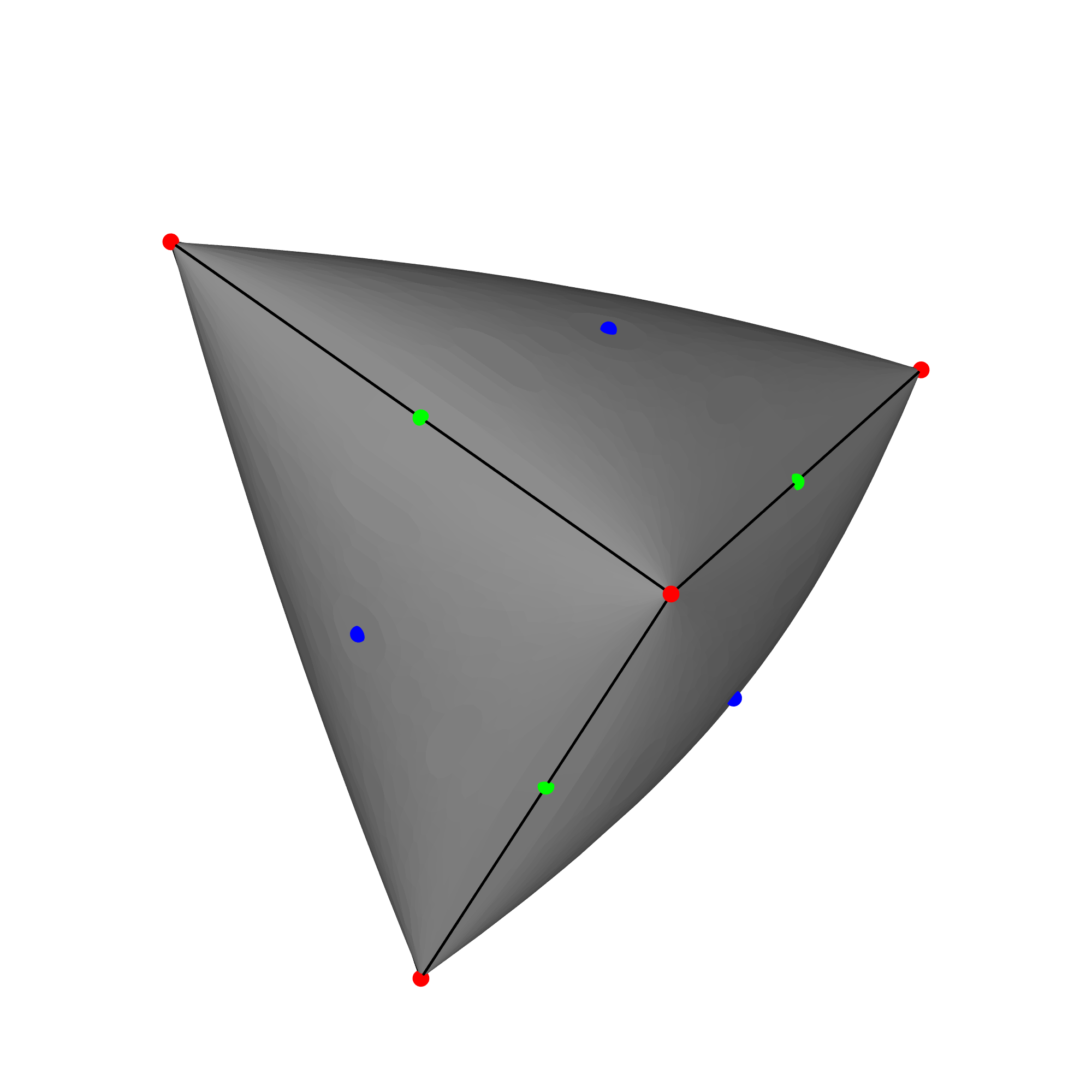
Figure 1: The elliptope ${\cal L}_{3}$. The highlighted points are the fixed points of $T$. Points in the elliptope correspond to certain positive semidefinite matrices (see Section 4). The red fixed points are irreducible matrices with rank 1, the blue fixed points are irreducible matrices with rank 2 and the green fixed points are reducible matrices with rank 2.

Let $n(x)$ be the normal direction at a smooth boundary point $x\in\Delta$. Then $x\in N(\Delta,x)$ when $x=\lambda n(x)$. In particular, $x$ is a fixed point exactly when the line through $x$ with direction $n(x)$ includes the origin.

Example 3 (Off-centered disk).

Figure 2 shows an example where $\Delta$ is an off-center disk. The disk contains the origin but not in its center. In this case there are two fixed points $A$ and $R$, where the line defined by the center of the disk and the origin crosses the boundary. Figure 2(a) illustrates the computation of $T(x)$ as the boundary point in a tangent line perpendicular to $x$. Figure 2(b) shows the result of fixed point iteration $x_{i+1}=T(x_{i})$ starting at $x_{0}$. Note how $x_{0}$ is near one fixed point ($R$) but the iteration converges to the other fixed point ($A$). In this case $A$ is an attractive fixed point, while $R$ is repelling (see Section 3.1). If we start the iteration anywhere except at $R$ the process converges to $A$. Note that if the origin is at the center of the disk then all boundary points are fixed points (neither attractive nor repelling).

Example 4 (Ellipse).

Figure 3 shows an example where $\Delta$ is an ellipse centered at the origin. In this case there are two attractive ($A_{1},A_{2}$) and two repelling ($R_{1},R_{2}$) fixed points. Each attractive fixed point is in the major axis of the ellipse. The repelling fixed points are in the minor axis.

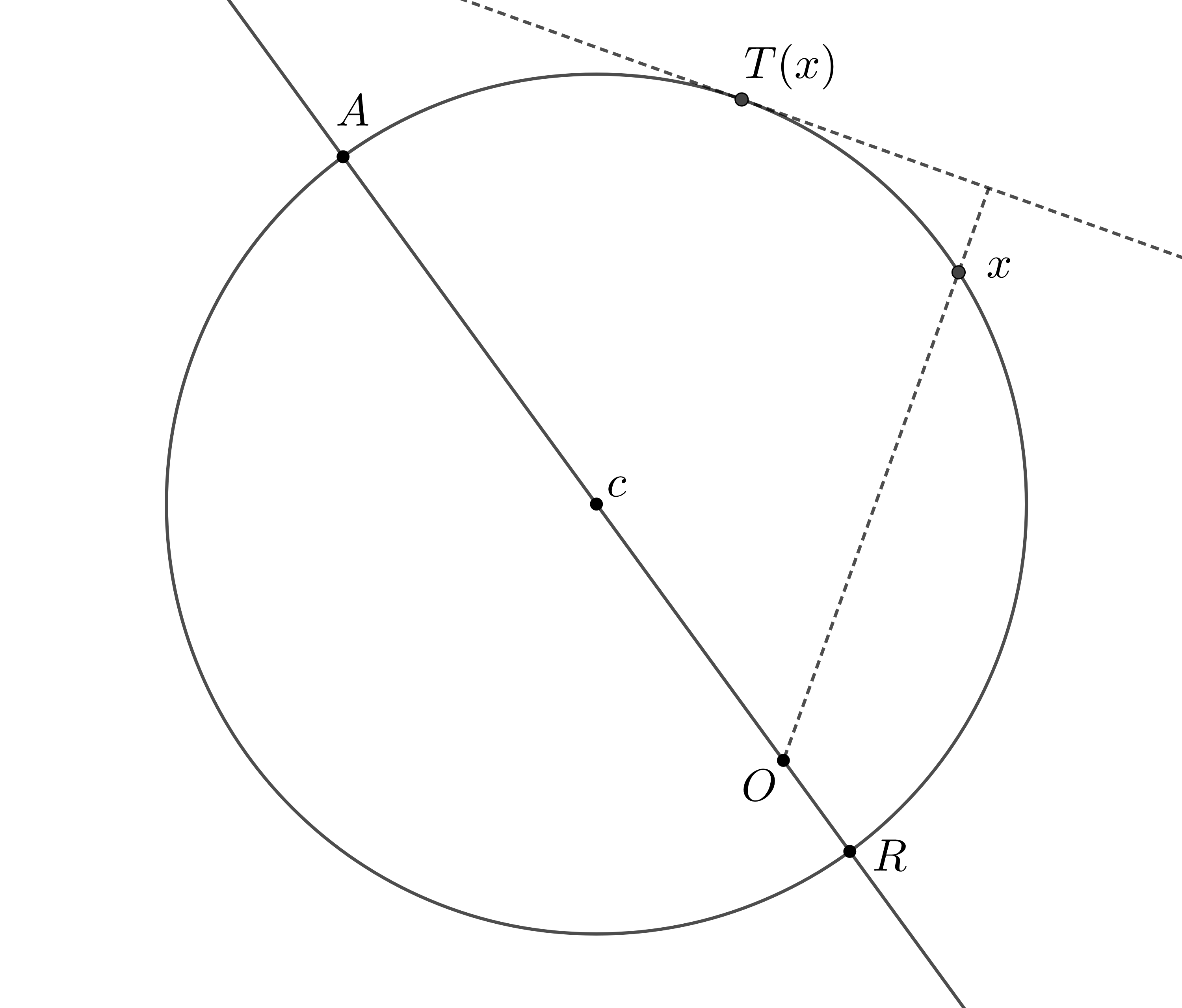
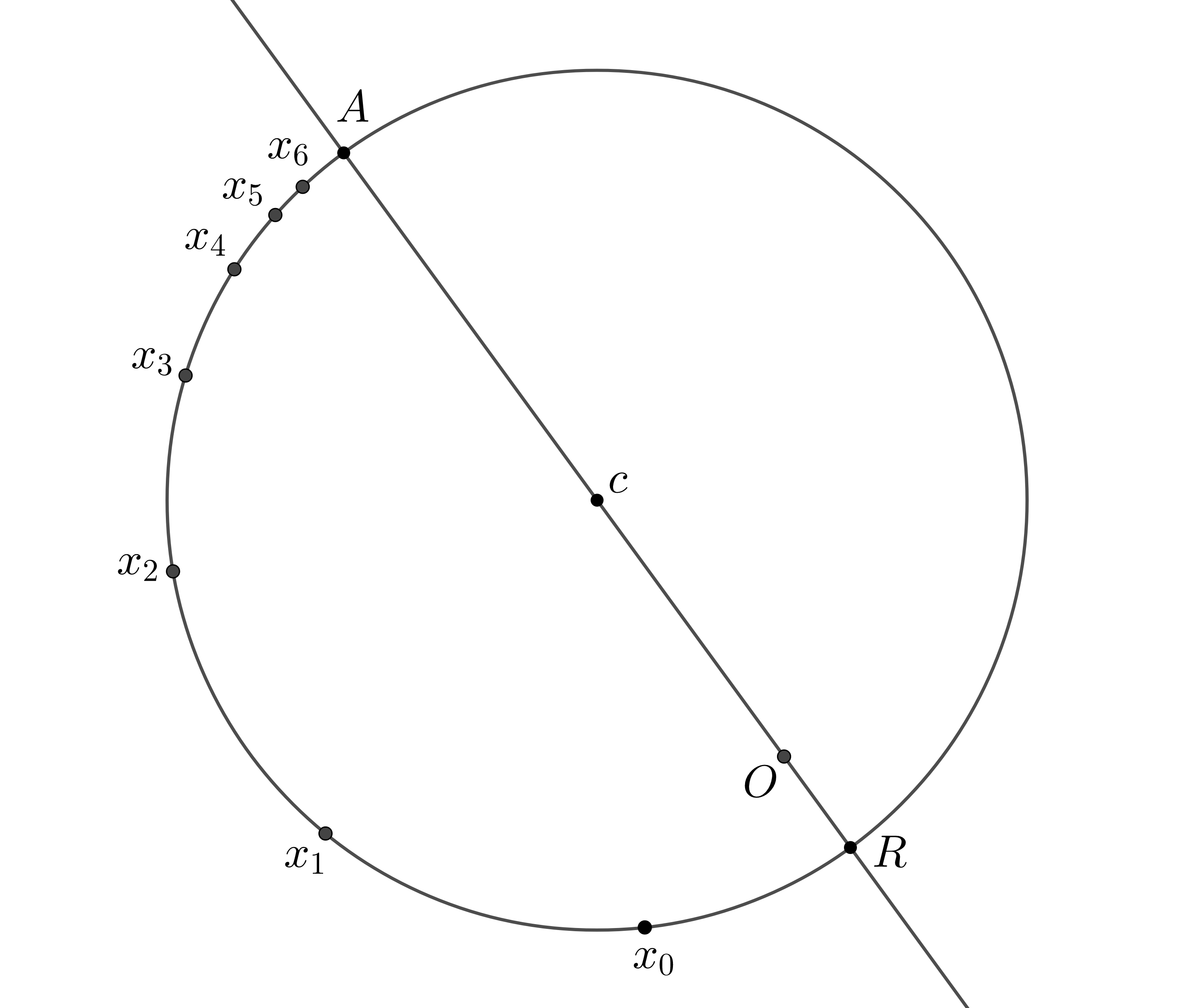
(a) (b)

Figure 2: (a) Illustration of the map $T$ and (b) fixed point iteration when $\Delta$ is an off-center disk. Here $c$ is the center of the disk while $O$ is the origin. The points $A$ and $R$ are the fixed points of $T$. Fixed point iteration converges to $A$ even when we start from a point closer to $R$. In this case $A$ is an attractive fixed point, while $R$ is a repelling fixed point.

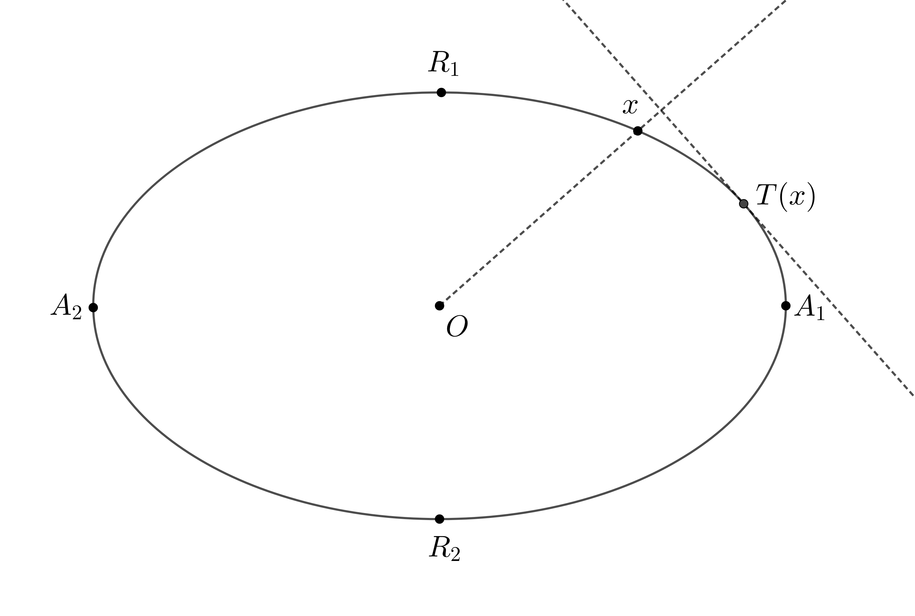
Figure 3: The fixed points of $T$ in an ellipse. Here the ellipse is centered at the origin $O$. There are two attractive $(A_{1},A_{2})$ and two repelling $(R_{1},R_{2})$ fixed points.

In Example 3 and Example 4 above we see that iteration with $T$ converges towards a fixed point, but never reaches it in a finite number of steps (unless we start at the fixed point). This is always the case when $\Delta$ is a region with smooth boundary. For such regions the normal cones are one dimensional and for $x$ to be a fixed point it must be that $x\in N(\Delta,x)$. Since no other boundary point can be in the normal cone at $x$, fixed point iteration cannot reach $x$ in a finite number of steps.

On the other hand, consider the case when $\Delta$ is a polytope. In this case fixed point iteration with $T$ always reaches a fixed point in a finite number of steps. For a generic point $x\in\Delta$, $T(x)$ is a vertex of the polytope, and iteration with $T$ defines a sequence of vertices with increasing norms. The set of vertices that are fixed points depends on the position of the origin. Fixed points can also exist in higher dimensional faces, but are then never attractive.

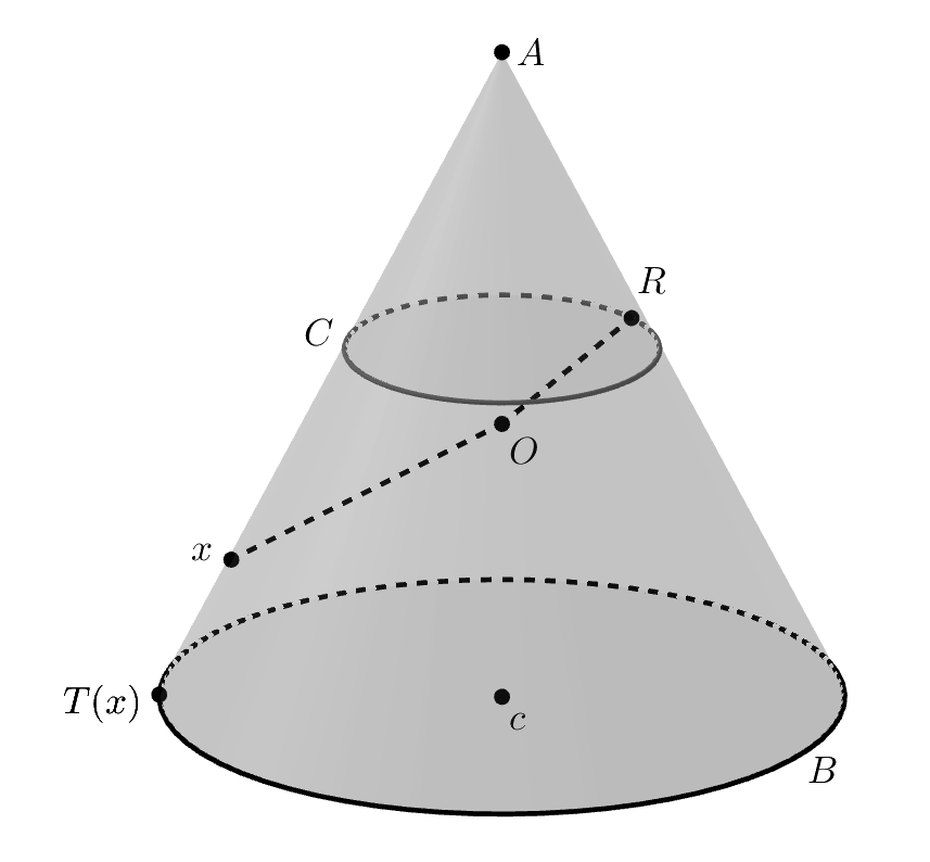
Figure 4: The fixed points of $T$ in a cone. Here $O$ is the origin while $c$ is the center of the base. The top of the cone is an attractive fixed point $A$. There is a circle of repelling fixed points $C$ in the middle of the cone. There is also a circle $B$ of fixed points at the base. Any point above $C$ maps to $A$ under $T$, while any point below $C$ maps to $B$. Fixed points in the base are not individually attractive or repelling, but together they form an attractive set.

Example 5 (Cone).

Figure 4 shows an example when $\Delta$ is a three-dimensional cone. In this case there is an attractive fixed point $A$ at the top of the cone. There is a circle $C$ in the middle of the cone and each point in $C$ is a repelling fixed point. We also have a circle $B$ of fixed points at the base. Any point above $C$ maps to $A$ under $T$ in a single step. Similarly any point below $C$ maps to $B$ in a single step. The map $T$ takes any point near $B$ to $B$ so we can see $B$ as an attractive set. However, the points in $B$ are not individually attractive or repelling.

3.1 Fixed Point Classification

Fixed point iteration defines a discrete dynamical system. There are several notions of stability for such systems and the notions we use throughout the paper are defined below (see, e.g., [11, 13]).

Definition 6.

A fixed point $x$ is attractive if $\exists\epsilon>0$ such that $||x-x_{0}||<\epsilon$ implies that iteration with $T$ starting at $x_{0}$ converges to $x$.

Definition 7.

A fixed point $x$ is repelling if $\exists\epsilon>0$ such that $||x-x_{0}||<\epsilon$ and $x_{0}\neq x$ implies there is an $n$ for which iteration with $T$ starting at $x_{0}$ leads to $x_{n}$ with $||x_{n}-x||>\epsilon$.

Consider a two-dimensional region $\Delta$ with smooth boundary. For any fixed point $x$ the tangent at $x$ is perpendicular to $x$. Therefore, the behavior of $T$ at a point $y$ sufficiently near $x$ depends only the curvature, $k(x)$, of the boundary at $x$. If $k(x)>1/||x||$ then $x$ is attractive. In this case the behavior of $T$ near $x$ is similar to the behavior of $T$ near the attractive fixed point in the off-center disk in Example 3. On the other hand, if $k(x)<1/||x||$ then $x$ is repelling. In this case the behavior of $T$ near $x$ is similar to the behavior of $T$ near the repelling fixed point in the off-center disk in Example 3.

In higher dimensions the situation is more subtle because the the boundary has multiple principal curvatures. In particular a fixed point may be behave like an attractive fixed point along one direction and like a repelling fixed point along another. A fixed point $x$ is attractive if all curvatures at $x$ are greater than $1/||x||$. Similarly a fixed point is repelling if all curvatures at $x$ are smaller than $1/||x||$.

4 Elliptope

For the remainder of the paper we study the fixed points and the fixed point iteration process in the special case of the elliptope, the study of which is motivated by SDP relaxations of combinatorial optimization problems (see, e.g., [12, 15]). We first prove an eigenvector-like relationship between points $x$ and $T(x)$. Theorem 15 builds on this relationship giving an algebraic characterization of the fixed points in the elliptope. In Section 4.2, we fully illustrate all of the fixed points in dimension $3$ and give an explicit construction of an infinite family of fixed points in dimension $4$. In terms of the iteration process, we classify the attractive fixed points of the elliptope as exactly its vertices in Theorem 20. Finally, we discuss how fixed point iteration can be used to approximately solve the closest vertex problem and to round the solutions of SDP relaxations.

Let ${\mathcal{S}}(n)\subset\mathbb{R}^{n\times n}$ be the set of $n$ by $n$ symmetric matrices.

Definition 8.

The elliptope ${\mathcal{L}}_{n}$ is the subset of matrices in ${\mathcal{S}}(n)$ that are positive semidefinite and have all $1$’s on the diagonal:

$${\mathcal{L}}_{n}=\{X\in{\mathcal{S}}(n)\,|\,X\succcurlyeq 0,X_{i,i}=1\}.$$

For a matrix $X\in{\cal L}_{3}$, $X$ has the form,

$$X=\begin{pmatrix}1&x&y\\ x&1&z\\ y&z&1\end{pmatrix}.$$

Therefore we can visualize $X$ as a point $(x,y,z)\in\mathbb{R}^{3}$.

Figure 1 shows the elliptope ${\cal L}_{3}$ and the fixed points of $T$. The red fixed points are irreducible matrices with rank 1 and correspond to the vertices of the elliptope, the blue points are irreducible matrices (see Definition 11) with rank 2 and the green points are reducible matrices with rank 2. Example 16 in Section 4.2 describes the fixed points of ${\cal L}_{3}$ in more detail.

As seen in Figure 1, the fixed points of ${\cal L}_{3}$ and their ranks are related to the geometry of the convex body. In general, the vertices of the elliptope are always fixed points of $T$. However, there are other fixed points that reflect different geometrical structure. The geometry of the elliptope and the nature of the fixed points becomes more complex in higher dimensions. For example, while the number of fixed points is finite for $n=3$, when $n>3$ there are already an infinite number of fixed points.

4.1 Fixed points in ${\mathcal{L}}_{n}$

It is well known that the matrices in ${\mathcal{L}}_{n}$ are precisely the Gram matrices of $n$ unit vectors in $\mathbb{R}^{n}$ ([14]). For example, for the matrix $X$ above, there must exist vectors $v_{1},v_{2},v_{3}\in\mathbb{R}^{3}$ with $||v_{i}||=1$, such that $x=v_{1}^{T}v_{1}$, $y=v_{2}^{T}v_{2}$, $z={v_{3}}^{T}v_{3}$. Considering the optimization defined by $T(M)$ and using the Gram matrix representation for the matrices in ${\mathcal{L}}_{n}$ we obtain the following result.

Lemma 9.

Let $M\in{\mathcal{S}}(n)$ and $X=T(M)$.

Suppose $X$ is the Gram matrix of $n$ unit vectors $(v_{1},\ldots,v_{n})$. Then,

• There exists real values $\alpha_{i}$ such that

  $$\sum_{j\neq i}M_{i,j}v_{j}=\alpha_{i}v_{i}.$$

• The vectors $(v_{1},\ldots,v_{n})$ are linearly dependent and $\operatorname*{rank}(X)<n$.

• There exists a diagonal matrix $D$ such that,

  $$MX=DX.$$

Proof.

For $n$ unit vectors $(u_{1},\ldots,u_{n})$ let $E(u_{1},\ldots,u_{n})=Y\cdot M$ where $Y$ is the Gram matrix of $(u_{1},\ldots,u_{n})$. For a single unit vector $u$ let

$$E_{i}(u)=E(v_{1},\ldots,v_{i-1},u,v_{i+1},\ldots,v_{n}).$$

Since $X=T(M)$ the unit vectors $(v_{1},\ldots,v_{n})$ maximize $E$. Therefore $v_{i}$ maximizes $E_{i}$. Using the method of Lagrange multipliers to maximize $E_{i}(u)$ subject to $||u||^{2}=1$ we see that

$$\nabla E_{i}(v_{i})=\lambda_{i}\nabla||v_{i}||^{2}\Leftrightarrow 2\sum_{j\neq i}M_{i,j}v_{j}=2\lambda_{i}v_{i}.$$

This proves part (a).

For part (b) note that if $\lambda_{i}\neq 0$ then $v_{i}$ is in the span of $\{v_{j}\,|\,j\neq i\}$. On the other hand, if $\lambda_{i}=0$ then $\{v_{j}\,|\,j\neq i\}$ are linearly dependent. Let $V$ be the matrix with $v_{i}$ in the $i$-th row. Since $X=VV^{T}$ we have $\operatorname*{rank}(X)<n$.

For part (c) let $D$ be the diagonal matrix where $D_{i,i}=\alpha_{i}+M_{i,i}$. By part (a) we have $MV=DV$. Multiplying by $V^{T}$ on both sides we obtain $MX=DX$. ∎

The relationship between $X=T(M)$ and $M$ defined by $MX=DX$ is similar to the notion of an eigenvector. A vector $v$ is an eigenvector of $M$ with eigenvalue $\lambda$ if $Mv=\lambda v$. The condition $MX=DX$ is analogous but we have a matrix $X$ instead of a vector $v$, and a diagonal matrix $D$ instead of a scalar $\lambda$. Although this notion of an “eigenmatrix” is natural it does not seem to appear in the literature before.

The next result is one direction of Theorem 15. We present this result now because it will be used for some of the intermediate results leading to the other direction.

Proposition 10.

Let $X$ be a fixed point of $T$. Then

$$X^{2}=DX$$

where $D$ is a diagonal matrix with,

$$D_{i,i}=\sum_{j}(X_{i,j})^{2}\geq 1.$$

Proof.

Lemma 9 implies $X^{2}=DX$. Since $X\in{\mathcal{L}}_{n}$ we know $X_{i,i}=1$. Therefore

$$D_{i,i}=(DX)_{i,i}=(X^{2})_{i,i}=\sum_{j}(X_{i,j})^{2}\geq(X_{i,i})^{2}=1.$$

∎

Definition 11.

A matrix $M\in{\mathcal{S}}(n)$ is irreducible if we cannot partition $\{1,\ldots,n\}$ into two sets $A$ and $B$ with $M_{i,j}=0$ whenever $i\in A$ and $j\in B$.

Proposition 12.

Let $X\in{\mathcal{L}}_{n}$ be an irreducible matrix with $X^{2}=DX$. Then $D=\gamma I$ with $\gamma\geq 1$.

Proof.

As in Proposition 10 we know $D_{i,i}\geq 1$. For $i\neq j$,

$$\frac{1}{D_{i,i}}\sum_{l=1}^{n}X_{i,l}X_{l,j}=X_{i,j}=X_{j,i}=\frac{1}{D_{j,j}}\sum_{l=1}^{n}X_{j,l}X_{l,i}.$$

If $X_{j,i}=X_{i,j}\neq 0$ then $D_{i,i}=D_{j,j}$. Since $X$ is irreducible this implies $D=\gamma I$. ∎

As an example consider the irreducible matrix $X$ and diagonal matrix $D$,

$$X=\begin{pmatrix}[r]1&-1&-1\\ -1&1&1\\ -1&1&1\end{pmatrix},\;D=\begin{pmatrix}[r]\frac{1}{3}&0&0\\ 0&\frac{1}{3}&0\\ 0&0&\frac{1}{3}\end{pmatrix}.$$

In this case $X^{2}=DX$ and $D=\frac{1}{3}I$.

Now consider the reducible matrix $X$ and diagonal matrix $D$ below,

$$X=\begin{pmatrix}[r]1&0&0\\ 0&1&1\\ 0&1&1\end{pmatrix},\;D=\begin{pmatrix}[r]1&0&0\\ 0&\frac{1}{2}&0\\ 0&0&\frac{1}{2}\end{pmatrix}.$$

In this case $X^{2}=DX$ but $D\neq\gamma I$ for any $\gamma$.

To characterize the fixed points of $T$ we use a result from [15] about the normal cones in ${\mathcal{L}}_{n}$.

Proposition 13 (Proposition 2.3 in [15]).

A matrix $Y$ is in the normal cone of ${\mathcal{L}}_{n}$ at $X$ if and only if $Y=D-M$ where $D$ is a diagonal matrix and $X\cdot M=0$

Note that the condition $X\cdot M=0$ is equivalent to $M=\sum_{j=1}^{p}w(j)w(j)^{\top}$ with $w(j)\in\ker(X)$.

Lemma 14.

Let $X$ be an irreducible matrix in ${\mathcal{L}}_{n}$ with rank $s$. Then $X$ is a fixed point of $T$ if and only if $X$ can be written as

$$X=\frac{n}{s}\sum_{i=1}^{s}v(i)v(i)^{\top},$$

where $\{v(1),\ldots,v(s)\}$ is an orthonormal set of vectors such that for all $j=1,\ldots,n$

$$\frac{n}{s}\sum_{i=1}^{s}v(i)_{j}^{2}=1.$$

Proof.

First, suppose that $X$ is a fixed point. Let $\{v(1),\ldots,v(s)\}$ be an orthonormal set of eigenvectors for $X$. Since $X$ is symmetric, we can write $X$ as

$$X=\sum_{i=1}^{s}\lambda_{i}v(i)v(i)^{\top}$$

where $\lambda_{i}>0$ is the eigenvalue associated with the eigenvector $v(i)$. Further, since $X$ is a fixed point, using Propositon 13, we can write $X=D-M$, where $D$ is a diagonal matrix and $M=\sum_{j=1}^{p}w(j)w(j)^{\top}$ with $w(j)\in\mathrm{ker}(X)$. Thus, for all $i=1,\ldots,s$

$$\lambda_{i}v(i)=Xv(i)=(D-M)v(i)=Dv(i).$$

This shows that $D_{j,j}=\lambda_{i}$ for all $j$ such that $v(i)_{j}\neq 0$. Since $X$ is irreducible, this implies that $\lambda_{i}=\lambda$ for all $i=1,\ldots,s$ and $D=\lambda I$. Further, for all $j=1,\ldots,n$

$$1=X_{j,j}=\lambda\sum_{i=1}^{s}v(i)_{j}^{2}.$$

Summing over all $j$, yields $n=\lambda s$ or $\lambda=n/s$. This completes the first direction of the proof.

Now suppose that $X$ can be written as

$$X=\frac{n}{s}\sum_{i=1}^{s}v(i)v(i)^{\top},$$

as above. Consider the matrix $M=\frac{n}{s}I-X$. Since $M$ is symmetric, we can write $M=\sum_{j=1}^{p}\alpha_{j}w(j)w(j)^{\top}$, where $\{w(1),\ldots,w(p)\}$ is a set of orthonormal eigenvectors of $M$ and $\alpha_{j}$ is the eigenvalue associated with $w(j)$. For all $j=1,\ldots,p$

$$\alpha_{j}w(j)=Mw(j)=\frac{n}{s}w(j)-Xw(j).$$

Thus, $w(j)$ is an eigenvector of $X$ as well. This shows that either $\alpha_{j}=n/s$ and $w(j)$ is in the kernel of $X$ or $\alpha_{j}=0$ (and we can remove these vectors from the sum defining $M$). Now Proposition 13 implies $X$ is a fixed point. ∎

We now prove our main result of this Section which characterizes the set of fixed points in ${\mathcal{L}}_{n}$.

Theorem 15.

Let $X$ be a matrix in ${\mathcal{L}}_{n}$. Then $X$ is a fixed point of $T$ if and only if

$$X^{2}=DX$$

where $D$ is a diagonal matrix.

Proof.

First consider the case where $X$ is an irreducible irreducible matrix in $\mathcal{L}_{n}$. Then we claim that $X$ is a fixed point if and only if $X^{2}=DX$ where $D$ is a diagonal matrix.

When $X$ is a fixed point Proposition 10 implies $X^{2}=DX$.

Now suppose $X^{2}=DX$. Since $X$ is irreducible $D=\gamma I$ with $\gamma\geq 1$. Let $\{v(1),,\ldots,v(s)\}$ be an orthonormal set of eigenvectors for $X$. Since $X$ is symmetric, we can write $X$ as

$$X=\sum_{i}^{s}\lambda_{i}v(i)v(i)^{\top}$$

where $\lambda_{i}>0$ is the eigenvalue associated with the eigenvector $v(i)$. For all $i=1,2,\ldots,s$

$$\lambda_{i}v(i)=Xv(i)=\frac{1}{\gamma}X^{2}v(i)=\frac{\lambda_{i}^{2}}{\gamma}v(i).$$

Thus, $\lambda_{i}=\lambda$ for all $i$ with $\lambda=\gamma$. For $j=1,2,\ldots,n$

$$1=X_{j,j}=\lambda\sum_{i=1}^{s}v(i)_{j}^{2}.$$

Summing over all $j$, yields $n=\lambda s$ or $\lambda=n/s$. Now Lemma 14 implies $X$ is a fixed point.

Next suppose $X$ is a fixed point that does not necessarily correspond to an irreducible matrix. Then $X^{2}=DX$ by Proposition 10.

Now suppose $X^{2}=DX$. For $A\subseteq\{1,\ldots,n\}$ and $M\in{\mathcal{S}}(n)$ let $M|_{A}$ be the submatrix of $M$ indexed by the rows and columns in $A$. Let $G=(V,E)$ be a graph with $V=\{1,\ldots,n\}$ and $E=\{\{i,j\}\,|\,X_{i,j}\neq 0\}$. Let $\{A_{1},\ldots,A_{k}\}$ be the connected components of $G$. Then each submatrix $X|_{A_{i}}$ is irreducible and $X_{r,s}=0$ if $r\in A_{i}$ and $s\in A_{j}$ with $i\neq j$. Each irreducible block of $X$ is square, symmetric, positive semidefinite, and has $1$’s in the diagonal. Therefore $X|_{A_{i}}\in{\mathcal{L}}_{|A(i)|}$.

Since $X^{2}=DX$ we have $(X|_{A_{i}})^{2}=(D|_{A_{i}})(X|_{A_{i}})$. Since $X|_{A_{i}}$ is irreducible, $X|_{A_{i}}$ is a fixed point in ${\mathcal{L}}_{|A_{i}|}$. We can use Proposition 13 to write $X|_{A_{i}}=L(i)-M(i)$ where $L(i)$ is diagonal and $X|_{A_{i}}\cdot M(i)=0$. Let $L$ be the $n\times n$ matrix with $L|_{A_{i}}=L(i)$ and zeros in other entries. Let $M$ be the $n\times n$ matrix with $M|_{A_{i}}=M(i)$ and zeros in other entries. Then $X=L-M$ with $L$ diagonal and $X\cdot M=0$. Now Proposition 13 implies $X$ is a fixed point. ∎

4.2 Examples

Here we consider two examples that illustrate the fixed points of $T$ in elliptopes of different dimensions. Example 16 describes all of the fixed points in ${\cal L}_{3}$.

Example 16.

Figure 1 illustrates the fixed points in ${\cal L}_{3}$. In this case there are finitely many fixed points. There are 4 irreducible fixed points with rank 1 corresponding to the vertices of ${\cal L}_{3}$ (shown as red points in Figure 1). The corresponding matrices are:

$$\begin{pmatrix}[r]1&-1&-1\\ -1&1&1\\ -1&1&1\end{pmatrix},\begin{pmatrix}[r]1&-1&1\\ -1&1&-1\\ 1&-1&1\end{pmatrix},\begin{pmatrix}[r]1&1&-1\\ 1&1&-1\\ -1&-1&1\end{pmatrix},\begin{pmatrix}[r]1&1&1\\ 1&1&1\\ 1&1&1\end{pmatrix}.$$

There are 6 reducible fixed points with rank 2 (shown as green points in Figure 1). Each of these fixed points is the average of two vertices and appear along an “edge” of ${\cal L}_{3}$. The corresponding matrices are:

$$\begin{pmatrix}[r]1&1&0\\ 1&1&0\\ 0&0&1\end{pmatrix},\begin{pmatrix}[r]1&-1&0\\ -1&1&0\\ 0&0&1\end{pmatrix},\begin{pmatrix}[r]1&0&1\\ 0&1&0\\ 1&0&1\end{pmatrix},\begin{pmatrix}[r]1&0&-1\\ 0&1&0\\ -1&0&1\end{pmatrix},\begin{pmatrix}[r]1&0&0\\ 0&1&1\\ 0&1&1\end{pmatrix},\begin{pmatrix}[r]1&0&0\\ 0&1&-1\\ 0&-1&1\end{pmatrix}.$$

Finally, there are 4 irreducible fixed points with rank 2, one for each “puffed face” in ${\cal L}_{3}$ (shown as blue points in Figure 1). Each of these fixed points equals $T(M)$ for a matrix $M$ that is the average of 3 vertices, the average itself does not lie on the boundary of ${\cal L}_{3}$. The corresponding matrices are:

$$\begin{pmatrix}[r]1&-\frac{1}{2}&-\frac{1}{2}\\ -\frac{1}{2}&1&-\frac{1}{2}\\ -\frac{1}{2}&-\frac{1}{2}&1\end{pmatrix},\begin{pmatrix}[r]1&-\frac{1}{2}&\frac{1}{2}\\ -\frac{1}{2}&1&\frac{1}{2}\\ \frac{1}{2}&\frac{1}{2}&1\end{pmatrix},\begin{pmatrix}[r]1&\frac{1}{2}&-\frac{1}{2}\\ \frac{1}{2}&1&\frac{1}{2}\\ -\frac{1}{2}&\frac{1}{2}&1\end{pmatrix},\begin{pmatrix}[r]1&\frac{1}{2}&\frac{1}{2}\\ \frac{1}{2}&1&-\frac{1}{2}\\ \frac{1}{2}&-\frac{1}{2}&1\end{pmatrix}.$$

While there are a finite number of fixed points in ${\cal L}_{3}$, there is an infinite set of fixed points in ${\mathcal{L}}_{n}$ for $n>3$. Example 17 illustrates an infinite family of fixed points in ${\cal L}_{4}$.

Example 17.

In ${\cal L}_{4}$, any value $-1<c<1$ leads to a distinct fixed point,

$$X(c)=\begin{pmatrix}[r]1&-\sqrt{1-c^{2}}&0&c\\ -\sqrt{1-c^{2}}&1&-c&0\\ 0&-c&1&-\sqrt{1-c^{2}}\\ c&0&-\sqrt{1-c^{2}}&1\end{pmatrix}.$$

In this case we have $X(c)=\frac{1}{2}X(c)^{2}$.

Although there can be an infinite number of fixed points in $\mathcal{L}_{n}$, there can only be a finite number of regular points which are fixed points, where a point is regular (or smooth) if it has a one-dimensional normal cone [15].

Lemma 18.

In ${\mathcal{L}}_{n}$ there is a finite number of regular points that are also fixed points.

Proof.

By definition, a regular point is an extreme point whose normal cone is 1-dimensional. By Proposition 13 the kernel of $X$ is 1-dimensional. Let $w$ be the eigenvector of $X$ with eigenvalue 0 scaled such that $||w||=1$. Then we can write $X$ as

$$X=D-M$$

where $M=\alpha ww^{\top}$, $\alpha>0$, and $D$ is a diagonal matrix. Then,

$$\vec{0} =Xw=(D-M)w=(D-\alpha ww^{\top})w=(D-\alpha I)w,$$

where the last equality holds since $w^{T}w=1$. Thus, if $w_{i}\neq 0$, then $D_{i,i}=\alpha$. Further, since $X_{i,i}=1$ we know that $M_{i,i}=\alpha-1$ if $w_{i}\neq 0$. We also know that $M_{i,i}=\alpha w_{i}^{2}$. Thus, either $w_{i}=0$ or $w_{i}=\pm\sqrt{1-1/\alpha}$, where $\alpha$ is set so that $||w||=1$.

This shows that the fixed points are a subset of those matrices whose kernel is spanned by some $w\in\{0,1,-1\}^{n}$. In particular, set $w\in\{0,1,-1\}^{n}$ and $M=\alpha ww^{\top}$ for some $\alpha$. Suppose that $w$ has $p$ non-zero entries. Then, $X\cdot M=0$ and $X=D-M$ imply that $p\alpha(1+\alpha)=p^{2}\alpha^{2}$ or $\alpha=1/(p-1)$. This shows the unique construction of $X$ from $w$. ∎

4.3 Iteration in ${\mathcal{L}}_{n}$ and the closest vertex problem

An important step in using a convex relaxation to solve a combinatorial optimization problem involves rounding a point $X$ in the convex body to an integer solution $Y$ that is feasible for the underlying combinatorial problem. In the classical SDP relaxation of max-cut the integer solutions are the $\{-1,+1\}$ symmetric matrices in ${\mathcal{L}}_{n}$ of rank 1 ([12]). An integer solution $Y$ defines a partition of $[n]$ into two sets, where $i$ is in the same set as $j$ if $Y_{i,j}=1$ and in a different set if $Y_{i,j}=-1$ The integer solutions for max-cut are exactly the vertices of ${\mathcal{L}}_{n}$ ([15]) and one can solve the rounding problem for the SDP relaxation by finding the closest vertex to a matrix $X\in{\mathcal{L}}_{n}$.

Fixed point iteration with $T$ defines a deterministic method for solving the rounding problem. In particular, fixed point iteration solves a sequence of relaxations to the closest vertex problem. Moreover, the vertices of ${\mathcal{L}}_{n}$, which define partitions, are precisely the attractive fixed points of $T$.

First note that

$$||X-Y||^{2}=X\cdot X+Y\cdot Y-2(X\cdot Y).$$

For a vertex $Y$, $Y\cdot Y=n^{2}$. Therefore we can find the vertex $Y$ that is closest to $X$ by maximizing $X\cdot Y$. Relaxing this problem to ${\mathcal{L}}_{n}$ gives an SDP relaxation to the closest vertex problem, defined by $Y=T(X)$.

If $Y=T(X)$ is vertex, then $Y$ is is the closest vertex to $X$. On the other hand, if $Y$ is not a vertex, we consider (recursively) the problem of finding the vertex $Z$ that is closest to $Y$. This involves iterating $T$ to compute $Z=T(Y)$. Thus fixed point iteration solves a sequence relaxations of the closest vertex problem.

To show the vertices are the only attractive fixed points we need the following Lemma.

Proposition 19.

Let $X$ be any fixed point that is not a vertex of ${\mathcal{L}}_{n}$. Then, there exists a curve $\hat{X}(\alpha)$ $(0\leq\alpha\leq 1)$ such that $\hat{X}(0)=X$ and $\hat{X}(\alpha)\cdot\hat{X}(\alpha)>X\cdot X$ when $\alpha>0$.

Proof.

Since $X$ is not a vertex, there exists $i\neq j$ such that $X_{i,j}\not\in\{-1,+1\}$ and $\sum_{l}(X_{i,l})^{2}\leq\sum_{l}(X_{j,l})^{2}$. Suppose $X$ is the Gram matrix of $\{v_{1},\ldots,v_{n}\}$. We will construct $\hat{X}(\alpha)$ by moving the vector $v_{i}$ towards either $v_{j}$ or $-v_{j}$.

We first consider the case that $X_{i,j}\geq 0$. In this case, we move $v_{i}$ towards $v_{j}$. For $0\leq\alpha\leq 1$, define the unit vector

$$\hat{v}_{i}(\alpha)=z_{\alpha}((1-\alpha)v_{i}+\alpha v_{j}),$$

where $z_{\alpha}=1/\sqrt{(1-\alpha)^{2}+\alpha^{2}+2\alpha(1-\alpha)X_{i,j}}>1$ is a normalization factor. Now define $\hat{X}(\alpha)$ to be the Gram matrix of $\{v_{1},\ldots,v_{i-1},\hat{v}_{i}(\alpha),v_{i+1},\ldots,v_{n}\}$. Note that for $l\neq i$,

$$\hat{X}_{i,l}(\alpha)=z_{\alpha}((1-\alpha)X_{i,l}+\alpha X_{j,l}).$$

We now analyze the value of $\hat{X}(\alpha)\cdot\hat{X}(\alpha)$ and compare it to $X\cdot X$.

$$\hat{X}(\alpha)\cdot\hat{X}(\alpha) =X\cdot X+2\sum_{l\neq i}(\hat{X}(\alpha)_{i,l})^{2}-2\sum_{l\neq i}(X_{i,l})^{2},$$

where

$$\sum_{l\neq i}(\hat{X}(\alpha)_{i,l})^{2} =\sum_{l\neq i}\frac{(1-\alpha)^{2}(X_{i,l})^{2}+\alpha^{2}(X_{j,l})^{2}+2\alpha(1-\alpha)X_{i,l}X_{j,l}}{(1-\alpha)^{2}+\alpha^{2}+2\alpha(1-\alpha)X_{i,j}}$$

$$=\frac{(1-\alpha)^{2}\sum_{l\neq i}(X_{i,l})^{2}+\alpha^{2}\sum_{l\neq i}(X_{j,l})^{2}+2\alpha(1-\alpha)\sum_{l\neq i}X_{i,l}X_{j,l}}{(1-\alpha)^{2}+\alpha^{2}+2\alpha(1-\alpha)X_{i,j}}.$$

Since $X$ is a fixed point, we know that $X^{2}=DX$ with $D_{i,i}=\sum_{l}(X_{i,l})^{2}$, which implies that

$$X_{i,j}=\frac{\sum_{l}X_{i,l}X_{j,l}}{\sum_{l}(X_{i,l})^{2}}.$$

Rearranging this expression,

$$\sum_{l\neq i}X_{i,l}X_{j,l}=X_{i,j}\sum_{l}(X_{i,l})^{2}-X_{i,j}=X_{i,j}\sum_{l\neq i}(X_{i,l})^{2}.$$

We can now see that

$$\sum_{l\neq i}(\hat{X}(\alpha)_{i,l})^{2} =\frac{(1-\alpha)^{2}\sum_{l\neq i}(X_{i,l})^{2}+\alpha^{2}\sum_{l\neq i}(X_{j,l})^{2}+2\alpha(1-\alpha)X_{i,j}\sum_{l\neq i}(X_{i,l})^{2}}{(1-\alpha)^{2}+\alpha^{2}+2\alpha(1-\alpha)X_{i,j}}.$$

Last, we note that

$$\sum_{l\neq i}(X_{j,l})^{2}=\sum_{l\neq j}(X_{j,l})^{2}+1-(X_{i,j})^{2}.$$

Overall, this shows that

$$\sum_{l\neq i}(\hat{X}(\alpha)_{i,l})^{2}\geq\frac{(1-\alpha)^{2}\sum_{l\neq i}(X_{i,l})^{2}+\alpha^{2}[1-(X_{i,j})^{2}+\sum_{l\neq j}(X_{j,l})^{2}]+2\alpha(1-\alpha)X_{i,j}\sum_{l\neq i}(X_{i,l})^{2}}{(1-\alpha)^{2}+\alpha^{2}+2\alpha(1-\alpha)X_{i,j}}$$

and $\hat{X}(\alpha)\cdot\hat{X}(\alpha)>X\cdot X$ if $\alpha\neq 0$. Moreover, $\hat{X}(\alpha)\cdot\hat{X}(\alpha)$ strictly increases as $\alpha$ increases.

When $X_{i,j}<0$ a similar argument leads to the desired curve if we move $v_{i}$ towards $-v_{j}$. ∎

Theorem 20.

The vertices of ${\mathcal{L}}_{n}$ are the attractive fixed points of $T$.

Proof.

Let $X$ be a vertex of ${\mathcal{L}}_{n}$ and $M\in{\mathcal{L}}_{n}$ with $||M-X||<1$. Then $|X_{i,j}-M_{i,j}|<1$. Since $X_{i,j}\in\{-1,+1\}$ the matrix $M$ has the same sign pattern as $X$. That is, for every $+1$ entry in $X$ the corresponding entry in $M$ is positive, and for $-1$ entry in $X$ the corresponding entry in $M$ is negative. If $Y\in{\mathcal{L}}_{n}$ then $|Y_{i,j}|\leq 1$. Therefore $Y\neq X\Rightarrow M\cdot X>M\cdot Y$. We conclude $T(M)=X$ and fixed point iteration from $M$ converges to $X$ in a single step.

Now suppose $X$ is not a vertex. Proposition 19 implies $\forall\epsilon>0$ $\exists Y$ with $||Y-X||<\epsilon$ and $Y\cdot Y>X\cdot X$. Since $T(Y)\cdot T(Y)\geq Y\cdot Y$, fixed point iteration from $Y$ cannot converge to $X$. ∎

In the proof above we show that if $M$ is a matrix with the same sign pattern as a vertex $X$, then $T(M)=X$. The set of matrices $M$ for which $T(M)=X$ was considered in [7] (related problems were also considered in [6]). More generally we would like to understand the set $S(X)$ for which fixed point iteration starting from $S(X)$ converges to $X$. In ${\cal L}_{3}$ fixed point iteration from a generic starting point always converges to the closest vertex. However, in higher dimensions fixed point iteration can converge to a vertex that is not closest to the starting point.

References

- [1] Farid Alizadeh. Interior point methods in semidefinite programming with applications to combinatorial optimization. SIAM journal on Optimization, 5(1):13–51, 1995.
- [2] M. D. Asic and D. D. Adamovic. Limit points of sequences in metric spaces. The American Mathematical Monthly, 77(6):613–616, 1970.
- [3] Boaz Barak, Jonathan A Kelner, and David Steurer. Rounding sum-of-squares relaxations. In Proceedings of the forty-sixth annual ACM symposium on Theory of computing, pages 31–40, 2014.
- [4] Heinz H Bauschke, Regina S Burachik, Patrick L Combettes, Veit Elser, D Russell Luke, and Henry Wolkowicz. Fixed-point algorithms for inverse problems in science and engineering. Springer, 2011.
- [5] Vasile Berinde. Iterative approximation of fixed points. Springer, 2007.
- [6] Diego Cifuentes, Sameer Agarwal, Pablo A Parrilo, and Rekha R Thomas. On the local stability of semidefinite relaxations. arXiv preprint arXiv:1710.04287, 2017.
- [7] Diego Cifuentes, Corey Harris, and Bernd Sturmfels. The geometry of SDP-exactness in quadratic optimization. Mathematical Programming, 182:399–428, 2020.
- [8] P. Felzenszwalb, C. Klivans, and A. Paul. Clustering with iterated linear optimization. Technical report. In preparation.
- [9] Marguerite Frank and Philip Wolfe. An algorithm for quadratic programming. Naval Research Logistics Quarterly, 3(1‐2):95–110, 1956.
- [10] Alan Frieze and Mark Jerrum. Improved approximation algorithms for max k-cut and max bisection. Algorithmica, 18(1):67–81, 1997.
- [11] Oded Galor. Discrete dynamical systems. Springer, 2007.
- [12] Michel Goemans and David Williamson. Improved approximation algorithms for maximum cut and satisfiability problems using semidefinite programming. Journal of the ACM, 42(6):1115–1145, 1995.
- [13] Richard Holmgren. A first course in discrete dynamical systems. Springer, 2000.
- [14] Monique Laurent. Cuts, matrix completions and graph rigidity. Mathematical Programming, 79(1-3):255–283, 1997.
- [15] Monique Laurent and Svatopluk Poljak. On a positive semidefinite relaxation of the cut polytope. Linear Algebra and its Applications, 223/224:439–461, 1995.
- [16] Prasad Raghavendra and David Steurer. How to round any CSP. In 50th Annual IEEE Symposium on Foundations of Computer Science, pages 586–594, 2009.
- [17] Cynthia Vinzant. What is a spectrahedron? Notices Amer. Math. Soc., 61(5):492–494, 2014.