Decaying Orbit of the Hot Jupiter WASP-12b: Confirmation with TESS Observations

Abstract

Theory suggests that the orbits of some close-in giant planets should decay due to tidal interactions with their host stars. To date, WASP-12b is the only hot Jupiter reported to have a decaying orbit, at a rate of 29$\pm$2 msec year^-1. We analyzed data from NASA’s Transiting Exoplanet Survey Satellite (TESS) to verify that WASP-12b’s orbit is indeed changing. We find that the TESS transit and occultation data are consistent with a decaying orbit with an updated period of 1.091420090$\pm$0.000000041 days and a decay rate of 32.53$\pm$1.62 msec year^-1. We find an orbital decay timescale of $\tau$ = P/$|\dot{P}|$ = 2.90$\pm$0.14 Myr. If the observed decay results from tidal dissipation, the modified tidal quality factor is Q’_⋆ = 1.39$\pm$0.15 $\times 10^{5}$, which falls at the lower end of values derived for binary star systems and hot Jupiters. Our result highlights the power of space-based photometry for investigating the orbital evolution of short-period exoplanets.

citnum [figure]subcapbesideposition=top [table]capposition=top

1 Introduction

Some exoplanetary systems exhibit temporal variations in their orbital parameters. Such systems provide valuable insights into their physical properties and the processes that cause the variations. Light curves of transiting planets can be used to search for transit timing variations (TTVs; Agol et al. 2005; Agol & Fabrycky 2018) and, less frequently, for variations in transit duration (Agol & Fabrycky 2018) and the impact parameter (Herman et al. 2018; Szabó et al. 2020). The presence of TTVs can indicate additional bodies in the system or an unstable orbit resulting from tidal forces of the star (e.g., Miralda-Escudé 2002; Mazeh et al. 2013). Also, TTVs in tightly packed multi-planetary systems have been detected and used to constrain the masses of planets in the system (e.g., Agol & Fabrycky 2018).

Theory suggests that short-period massive planets orbiting stars with surface convective zones may exchange energy with their host stars through tidal interactions, causing the host star to spin faster and the planet’s orbit to decay (e.g., Lin et al. 1996; Chambers 2009; Lai 2012; Penev et al. 2014; Barker 2020). As the planet’s orbit decays over millions of years, its orbital period will change by a small, yet potentially detectable amount. Observations of this decay are now possible because some hot Jupiter systems have been monitored for decades. Such measurements enhance our understanding of the hot Jupiter population (e.g. Jackson et al. 2008; Hamer & Schlaufman 2019).

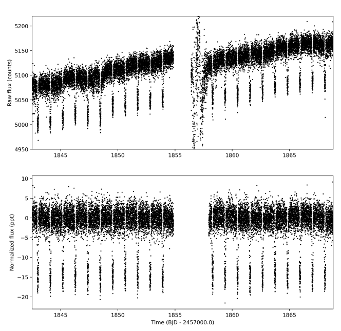
Figure 1: TESS light curve of WASP-12b in Sector 20. Top: Raw simple aperture photometry light curves. Bottom: Detrended Presearch Data Conditioning (PDC) time series.

Currently, WASP-12b is one of the few hot Jupiters confirmed to have a varying period. It orbits a G0 star with a short period of one day (Hebb et al. 2009). Since its discovery in 2009, WASP-12b’s orbital parameters (e.g., Campo et al. 2011; Maciejewski et al. 2016) and atmosphere (e.g., Croll et al. 2011; Stevenson et al. 2014; Sing et al. 2016) have been studied extensively. Observations with the Cosmic Origins Spectrograph (COS) on the Hubble Space Telescope reveal an early ingress in the near-ultraviolet (Fossati et al. 2010; Haswell et al. 2012; Nichols et al. 2015). An escaping atmosphere was suggested as the cause of the early ingress (e.g., Lai et al. 2010; Bisikalo et al. 2013; Turner et al. 2016a). Maciejewski et al. (2016) were the first to report evidence of a decreasing orbital period for WASP-12b. At the time, the cause of the changing orbit was uncertain, and could be ascribed to orbital decay, apsidal precession, or the Romer effect. Follow-up observations confirmed the changing orbital period, with models slightly favoring orbital decay as the cause (Patra et al. 2017; Maciejewski et al. 2018; Bailey & Goodman 2019). Recently, using new transit, occultation and radial velocity observations, Yee et al. (2020) presented strong evidence that WASP-12b’s period variation is caused by orbital decay. The decay rate has been constrained to between 20-30 milliseconds/yr.

Motivated by these indications of WASP-12b’s changing period, we use NASA’s Transiting Exoplanet Survey Satellite (TESS; Ricker et al. 2015) observations to verify its orbital decay, and derive updated orbital parameters and planetary properties. TESS is well suited for our study because it provides high-precision time-series data, ideal for searching for TTVs (e.g. Hadden et al. 2019; von Essen et al. 2020; Ridden-Harper et al. 2020).

2 Observations and Data Reduction

TESS observed WASP-12b in Sector 20 (December 24, 2019 to January 20, 2020; Figure 1). These observations were processed by the Science Processing Operations Center (SPOC) pipeline (Jenkins et al., 2016). The final product of the SPOC pipeline are light curves corrected for systematics that can be used to characterize transiting planets. All of the SPOC data products are publicly accessible from the Mikulski Archive for Space Telescopes (MAST). The Presearch Data Conditioning (PDC) component of the SPOC pipeline corrects the light curves for pointing or focus related instrumental signatures, discontinuities resulting from radiation events in the CCD detectors, outliers, and flux contamination. We use the PDC light curve for the analysis in this paper, however a known issue results in the SPOC pipeline overestimating the uncertainties for some light curves, including that of WASP-12b. Therefore, it is recommended that the uncertainties be estimated from the scatter (Barclay, T., private communication), until the data is reprocessed with an updated pipeline (data released after DR 38 should be unaffected). To do this, we used the standard deviation of the entire out-of-transit baseline as the uncertainty. Using smaller out-of-transit baselines surrounding only a few transits did not significantly change the standard deviation, indicating that the noise is relatively constant. The raw light curve from the SPOC and detrended PDC light curve are shown in Figure 1.

(a)

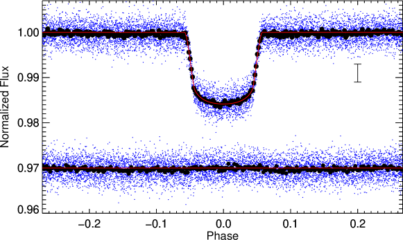
(b)

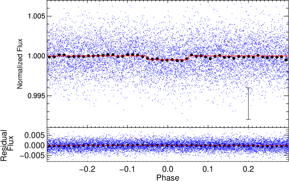
Figure 2: Phased folded transit (panel a) and occulation (panel b) light curves of WASP-12b from TESS. The unbinnned and binned data are shown in blue and black, respectively. The binned transit and occulation data have been binned by 2 and 18 minutes, respectively. The best-fitting model obtained from the EXOplanet MOdeling Package (EXOMOP) is shown as a solid red line. The residuals (light curve - model) are shown below the light curve.

3 Data Analysis

3.1 Transit Modeling

We modeled the TESS transits of WASP-12b with the EXOplanet MOdeling Package (EXOMOP; Pearson et al. 2014; Turner et al. 2016c, 2017) to find a best-fit. EXOMOP creates a model transit using the analytic equations of Mandel & Agol (2002) and the data are modeled using a Differential Evolution Markov Chain Monte Carlo (DE-MCMC; Eastman et al. 2013) analysis. To account for red noise in the light curve, EXOMOP incorporates the residual permutation, time-averaging, and wavelet methods. More detailed descriptions of EXOMOP can be found in Pearson et al. (2014) and Turner et al. (2016b).

Each transit in the TESS data (lower panel of Figure 1) was modeled with EXOMOP independently. We used 20 chains and 20⁶ links for the DE-MCMC model and ensure chain convergence (Ford 2006) using the Gelman-Rubin statistic (Gelman & Rubin 1992). The mid-transit time ($T_{c}$), planet-to-star radius ($R_{p}/R_{*}$), inclination ($i$), and scaled semi-major axis ($a/R_{*}$) are set as free parameters for every transit. The period ($P_{orb}$) and linear and quadratic limb darkening coefficients are fixed during the analysis. The linear and quadratic limb darkening coefficients used in the modeling were set to 0.2131 and 0.3212 (taken from Claret 2017), respectively.

The parameters derived for every TESS transit event can be found in Table 4. The modeled light curves for each individual transit can be found in Figures 4–7 in Appendix A. All parameters for each transit event are consistent within 2$\sigma$ of every other transit.

To obtain the final fitted parameters, the light curve of WASP-12b was phase-folded at each derived mid-transit time and modeled with EXOMOP. The phase-folded light curve and model fit can be found in Figure 2. We use the light curve model results combined with literature values to calculate the planetary mass (M_b; Winn 2010), radius (R_b), density ($\rho_{b}$), equilibrium temperature (T_eq), surface gravity ($\log{g_{b}}$; Southworth et al. 2007), orbital distance ($a$), inclination ($i$), Safronov number ($\Theta$; Safronov 1972; Southworth 2010), and stellar density ($\rho_{\ast a}$; Seager & Mallén-Ornelas 2003). The planet properties and transit ephemeris we derived for WASP-12b are shown in Table 1. All the planetary parameters are consistent with their discovery values (Hebb et al., 2009) but their precision is greatly improved.

Table 1: Physical properties of WASP-12b derived from the light curve modeling of the TESS data

Parameter	units	value	1 $\sigma$ uncertainty
Rp/R∗		0.1166445	0.0000097
a/R∗		3.1089	0.0014
$\delta$occ		0.00048	0.00010
Inclination	∘	84.955	0.037
Duration	mins	178.60	0.14
b		0.2734	0.0020
Rb	RJup	1.884	0.057
Mb	MJup	1.46	0.27
$\rho_{b}$	g cm-3	0.271	0.056
$\log{g_{b}}$	cgs	2.38	0.39
$\rho_{\ast a}$	g cm-3	0.477	0.026
Teq	K	2551	56
$\Theta$		0.0260	0.0053
a	au	0.02399	0.00072

3.2 Occultation Modeling

The TESS occultation was also modeled with EXOMOP to find the best-fit parameters. The light curve we fit was obtained by phase-folding all the data about the secondary eclipse using the first TESS transit as the reference transit time. We were unable to see or fit individual occulations as they were too shallow. Again, we used 20 chains and 20⁶ links for the DE-MCMC model and ensure chain convergence using the Gelman-Rubin statistic. The mid-occulation time (T_occ) and occultation depth ($\delta$_occ) were set as free parameters. The inclination, period, and scaled semi-major axis were fixed to the values obtained from the phase-folded transit curve (Table 1). The linear and quadratic limb darkening coefficients were both set to zero. We find a T_occ = 2458843.55034$\pm$0.00088 BJD_TDB for the first epoch (E=2325) in the TESS observations and $\delta$_occ=0.00048$\pm$0.00010. The results of the analysis do not change whether we use the first epoch or the middle epoch of the TESS data.

3.3 Timing

For the timing analysis, we combined the TESS transit and occultation data with the all the prior transit and occultation times complied by Yee et al. (2020). All the transit and occultation times used in this analysis can be found in Table 2. This table is available in its entirety in machine-readable form online.

Similar to what was done in Yee et al. (2020) and Patra et al. (2017), we fit the timing data to three different models. The first model is the standard constant period formalization:

$$t_{\text{tra}}(E)= T_{c,0}+P_{\text{orb}}\times E,$$ (1)

$$t_{\text{occ}}(E)= T_{c,0}+\frac{P_{\text{orb}}}{2}+P_{orb}\times E,$$ (2)

where $T_{0}$ is the reference transit time, $P_{orb}$ is the orbital period, $E$ is the transit epoch, and $T_{tra}(E)$ is the calculated transit time at epoch $E$.

The second model assumes that the orbital period is changing uniformly over time:

$$t_{\text{tra}}(E)= T_{c,0}+P_{orb}\times E+\frac{1}{2}\frac{\mathrm{d}P_{orb}}{\mathrm{d}E}E^{2},$$ (3)

$$t_{\text{occ}}(E)= T_{c,0}+\frac{P_{orb}}{2}+P_{orb}\times E+\frac{1}{2}\frac{\mathrm{d}P_{orb}}{\mathrm{d}E}E^{2},$$ (4)

where $\mathrm{d}P_{orb}/\mathrm{d}E$ is the decay rate.

The third model assumes the planet is precessing uniformly (Giménez & Bastero 1995):

$$t_{\text{tra}}(E)= T_{c,0}+P_{s}\times E-\frac{eP_{a}}{\pi}\cos{\omega(N)},$$ (5)

$$t_{\text{occ}}(E)= T_{c,0}+\frac{P_{orb}}{2}+P_{s}\times E+\frac{eP_{a}}{\pi}\cos{\omega(N)},$$ (6)

$$\omega(N)= \omega_{0}+\frac{\mathrm{d}\omega}{\mathrm{d}E}E,$$ (7)

$$P_{s}= P_{a}\left(1-\frac{1}{2\pi}\frac{\mathrm{d}\omega}{\mathrm{d}E}\right),$$ (8)

where $e$ is a nonzero eccentricity, $\omega$ is the argument of pericenter, P_s is the sidereal period and P_a is the anomalistic period.

Event	Midtime	Error	Epoch	Source
Type	BJDTDB	days
tra	2458843.00493	0.00054	2325	This Paper
tra	2458844.09660	0.00052	2326	This Paper
tra	2458845.18785	0.00046	2327	This Paper
tra	2458846.27971	0.00054	2328	This Paper
tra	2458847.37083	0.00051	2329	This Paper
tra	2458848.46238	0.00049	2330	This Paper
tra	2458849.55308	0.00043	2331	This Paper
tra	2458850.64512	0.00053	2332	This Paper
tra	2458851.73590	0.00057	2333	This Paper
tra	2458852.82819	0.00038	2334	This Paper
tra	2458853.91924	0.00047	2335	This Paper
tra	2458858.28450	0.00061	2339	This Paper
tra	2458859.37732	0.00055	2340	This Paper
tra	2458860.46816	0.00044	2341	This Paper
tra	2458861.55803	0.00049	2342	This Paper
tra	2458862.65047	0.00057	2343	This Paper
tra	2458863.74203	0.0006	2344	This Paper
tra	2458864.83395	0.00044	2345	This Paper
tra	2458865.92421	0.0005	2346	This Paper
tra	2458867.01609	0.00051	2347	This Paper
tra	2458868.10763	0.00046	2348	This Paper
occ	2458843.55034	0.00088	2325	This Paper

Table 2: All WASP-12b Transit and Occultation Times

For all the three models, we found the best-fitting model parameters using a DE-MCMC analysis. We used 20 chains and 20⁶ links in the model and again we ensure chain convergence using the Gelman-Rubin statistic. The results of timing model fits can be found in Table 3.

Figure 3 shows the transit and occultation timing data fit with the orbital decay and apsidal precession models. In this figure, the best-fit constant-period model has been subtracted from the timing data. For the TESS transits alone (panel a), the orbital decay model fits the data slightly better than the precession model. When all the available transit data are combined (panel b), then it is more apparent that orbital decay is favored as the cause. The occultation data also favor the orbital decay model (panel c), with the new TESS data point important for discriminating between the two possibilities.

Table 3: Best-Fit Parameters for Timing Models

Parameter	Symbol	units	value	1 $\sigma$ uncertainty
Constant Period Model
Period	P${}_{\text{orb}}$	days	1.091419426	0.000000022
Mid-transit time	Tc,0	BJDTDB	2456305.455519	0.000026
Ndof			182
$\chi$${}_{min}^{2}$			576.08
BIC			586.47
Orbital Decay Model
Period	P${}_{\text{orb}}$	days	1.091420090	0.000000041
Mid-transit time	Tc,0	BJDTDB	2456305.455795	0.000038
Decay Rate	dP/dE	days/orbit	-9.45$\times$10-10	4.7$\times$10-11
Decay Rate	dP/dt	msec/yr	-32.53	1.62
Ndof			183
$\chi$${}_{min}^{2}$			188.71
BIC			204.30
Apsidal Precession Model
Sidereal Period	Ps	days	1.091419419	0.000000052
Mid-transit time	Tc,0	BJDTDB	2456305.45481	0.00011
Eccentricity	e		0.00363	0.00025
Argument of Periastron	$\omega$0	rad	2.447	0.077
Precession Rate	d$\omega$/dN	rad/orbit	0.000963	0.000040
Ndof			185
$\chi$${}_{min}^{2}$			212.75
BIC			238.72

Thus, we find that the orbital decay model fits the timing data the best (Table 3, Figure 3). The fact that the constant-period model does not fit the data is consistent with previous findings (Maciejewski et al. 2016, Patra et al. 2017, Yee et al. 2020). The orbital decay and apsidal precession models fit the data with a minimum chi-squared ($\chi$${}_{min}^{2}$) of 188.71 and 212.75, respectively. We use the Bayesian Information Criterion (BIC) to assess the preferred model. The BIC is defined as

$$BIC=\chi^{2}+k\ln{(N_{pts})},$$ (9)

where $k$ is the number of free parameters in the model fit and $N_{pts}$ is the number of data points. The power of the BIC is the penalty for a higher number of fitted model parameters, making it a robust way to compare different best-fit models. The preferred model is the one that produces the lowest BIC value. We find that the orbital decay model is the preferred model with a $\Delta$(BIC) = 34.42. We can relate the $\Delta$(BIC) and the Bayes factor $B$ assuming a Gaussian distribution for the posteriors:

$$B=\exp[-\Delta(BIC)/2]=3\times 10^{7}.$$ (10)

Therefore, the orbital decay model is overwhelming the preferred interpretation of the observed timing residuals.

(a)

(a)

(b)

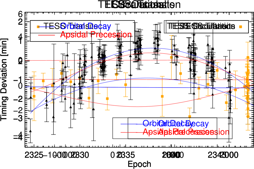
(b)

(c)

(c)

Figure 3: Transit (panels a and b) and occultation (panel c) timing variations after subtracting the data with a constant-period model. The filled black triangles are the data points complied from Yee et al. (2020) and the square orange points are from the TESS data in this paper. All the transit and occultation times can be found in Table 2. The orbital decay and apsidal precession models are shown as the blue and red lines, respectively.

4 Discussion

From our analysis, we derive an updated period of 1.091420090$\pm$0.000000041 days and a decay rate of 32.53$\pm$1.62 msec year^-1. Our results indicate an orbital decay timescale of $\tau=P/|\dot{P}|=2.90\pm 0.14$ Myr, slightly shorter than the value derived by Yee et al. (2020) of $3.25^{+0.24}_{-0.21}$ Myr. The mass-loss rate required to explain the early ingress of WASP-12b in the near-UV is $\sim 3\times 10^{14}gs^{-1}$, which corresponds to a mass-loss timescale of $M_{p}/\dot{M}_{p}\sim 300$ Myr (Lai et al., 2010; Jackson et al., 2017), which is about two orders of magnitude longer than the orbital decay timescale. Therefore, the orbital decay timescale is the dominant timescale for the evolution of WASP-12b.

Our analysis strengthens the case for the changing period of WASP-12b being produced by tidal decay. In this scenario, WASP-12b’s orbital energy is dissipated by tides within its host star. The effectiveness of such tidal dissipation is quantified conveniently by the modified tidal quality factor, $Q^{\prime}_{\star}$, which is related to the star’s tidal quality factor, $Q_{\star}$ by

$$Q^{\prime}_{\star}=\frac{Q_{\star}}{\frac{2}{3}k_{2}},$$ (11)

where $k_{2}$ is a Love number.

Assuming that the planet mass is constant, the rate of change of WASP-12b’s orbital period, $\dot{P}$, can be related to its host star’s modified tidal quality factor by the constant-phase-lag model of Goldreich & Soter (1966), defined as

$$\dot{P}=-\frac{27\pi}{2Q^{\prime}_{\star}}\left(\frac{M_{p}}{M_{\star}}\right)\left(\frac{R_{\star}}{a}\right)^{5},$$ (12)

where $M_{p}$ is the mass of the planet, $M_{\star}$ is the mass of the host star, $R_{\star}$ is the radius of the host star and $a$ is the semi-major axis of the planet.

By substituting our derived value of $\dot{P}$ and the remaining values from Table 1 and Hebb et al. (2009), we find a modified tidal quality factor of Q’_⋆ = 1.39$\pm$0.15 $\times$ 10⁵. This value is slightly lower than the value derived by Yee et al. (2020) of Q’_⋆ = 1.75${}^{+0.13}_{-0.11}$ $\times$ 10⁵, and is generally at the lower end of observed values for binary star systems ($10^{5}-10^{7}$; Meibom et al., 2015) and hot Jupiters ($10^{5}-10^{6.5}$; Jackson et al., 2008; Husnoo et al., 2012; Barker, 2020). Additionally, Hamer & Schlaufman (2019) found that hot Jupiter host stars tend to be young, implying that such planets spiral into their stars during the main sequence phase, requiring Q’_⋆ $\lesssim$ 10⁷.

It is not yet clear how to account for the observed low values of $Q^{\prime}_{\star}$ because, in general, theoretically derived values for $Q^{\prime}_{\star}$ tend to be higher ($10^{7}-10^{10}$; Ogilvie 2014, and references therein). Weinberg et al. (2017) show that if WASP-12 were a sub-giant star, nonlinear wave-breaking of the dynamical tide near the stellar core would lead to $Q^{\prime}_{\star}\sim 2\times 10^{5}$, which is reasonably close to the observed value of $Q^{\prime}_{\star}$ = 1.56 $\times 10^{5}$. However, Bailey & Goodman (2019) found that the observed characteristics of WASP-12 are more consistent with it being a main-sequence star, so more theoretical work could be informative.

WASP-12b is the only exoplanet for which there is robust evidence of tidal orbital decay. However, WASP-103b, KELT-16b, and WASP-18b are also predicted to exhibit comparable rates of tidal decay (Patra et al., 2020). Hence, additional data could reveal whether they indeed exhibit hitherto undetected tidal decay or whether the theoretical predictions need to be improved. Timing observations of additional systems are warranted because they help us understand the formation, evolution and ultimate fate of hot Jupiters (e.g. Jackson et al. 2008; Hamer & Schlaufman 2019).

5 Conclusions

We analyzed TESS data of WASP-12b to characterize the system and to verify that the planet is undergoing orbital decay. Our TESS transit and occultation timing investigations confirm that the planet’s orbit is changing. We compare our timing residuals to orbital decay and apsidal precession models, and our analysis highly favors the orbital decay scenario with a Bayes factor of 3$\times 10^{7}$. We find an updated period of 1.091420090$\pm$0.000000041 days and a decay rate of 32.53$\pm$1.62 msec year^-1. Our finding indicates an orbital decay lifetime of 2.90$\pm$0.14 Myr, shorter than the estimated mass-loss timescale of 300 Myr. We also update the planetary physical parameters and greatly improve on their precision. Our study highlights the power of long-term high-precision (both in flux and timing accuracy) ground and space-based transit and occultation observations for understanding orbital evolution of close-in giant planets.

Appendix A Transit fits to individual TESS transit events

The parameters for each transit fit can be found in Table 4. The light curves and EXOMOP model fits can be found in Figures 4–7.

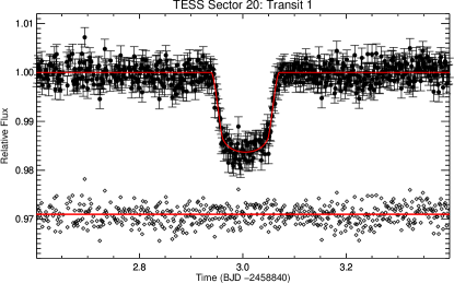
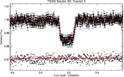
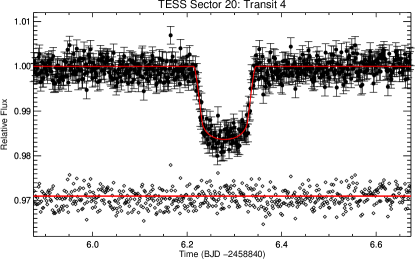
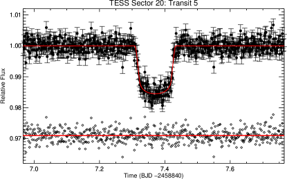
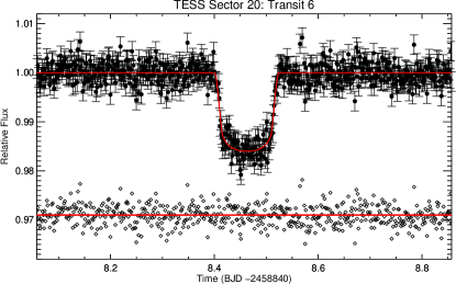
Figure 4: Individual TESS transit events (1-6) from Sector 20 of WASP-12b. The best-fitting model obtained from the EXOplanet MOdeling Package (EXOMOP) is shown as a solid red line. The residuals (light curve - model) are shown below the light curve.

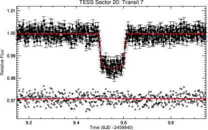
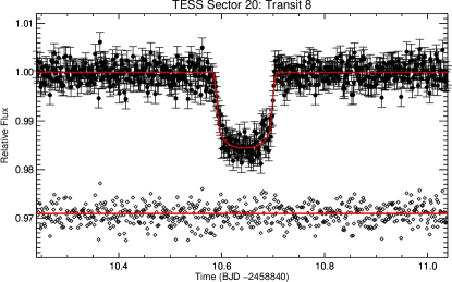
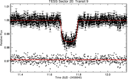
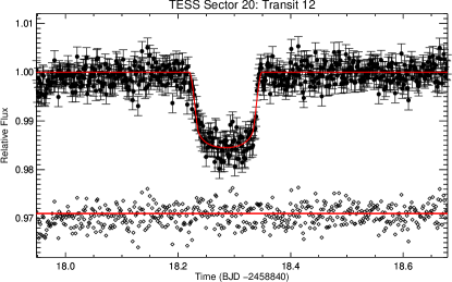
Figure 5: Individual TESS transit events (7-12) from Sector 20 of WASP-12b. Other comments are the same as Figure 4.

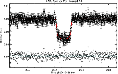
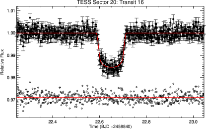
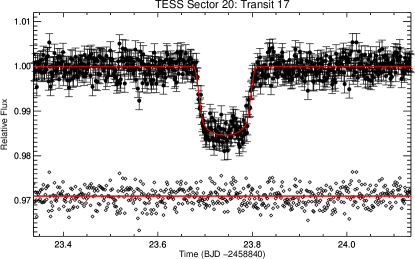
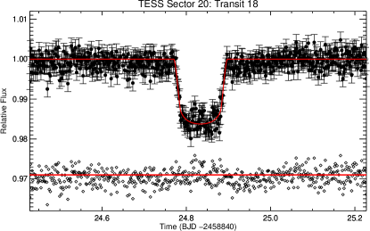
Figure 6: Individual TESS transit events (13-18) from Sector 20 of WASP-12b. Other comments are the same as Figure 4.

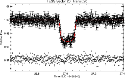
Figure 7: Individual TESS transit events (19-21) from Sector 20 of WASP-12b. Other comments are the same as Figure 4.

Table 4: Individual TESS Sector 20 transit parameters for WASP-12b derived using EXOMOP

Transit	0	1	2
Tc (BJDTDB-2458840)	3.00484$\pm$0.00054	4.09663$\pm$0.00053	5.18779$\pm$0.00053
Rp/R∗	0.1229$\pm$0.0020	0.1207$\pm$0.0020	0.1195$\pm$0.0019
a/R∗	2.67$\pm$0.20	2.95$\pm$0.26	2.92$\pm$0.22
Inclination (∘)	77.25$\pm$3.08	81.26$\pm$2.72	81.42$\pm$1.98
Duration (mins)	185.98$\pm$3.00	177.89$\pm$2.87	180.00$\pm$2.83
Transit	3	4	5
Tc (BJDTDB-2458840)	6.27961$\pm$0.00056	7.37087$\pm$0.00052	8.46245$\pm$0.00047
Rp/R∗	0.1220$\pm$0.0022	0.1175$\pm$0.0018	0.1190$\pm$0.0013
a/R∗	2.76$\pm$0.16	3.05$\pm$0.23	3.14$\pm$0.11
Inclination (∘)	79.25$\pm$1.95	83.29$\pm$4.67	84.91$\pm$5.27
Duration (mins)	185.98$\pm$2.83	175.96$\pm$2.83	175.96$\pm$2.84
Transit	6	7	8
Tc (BJDTDB-2458840)	9.55312$\pm$0.00043	10.64494$\pm$0.00052	11.73596$\pm$0.00055
Rp/R∗	0.1163$\pm$0.0010	0.1169$\pm$0.0015	0.1188$\pm$0.0023
a/R∗	3.23$\pm$0.12	3.15$\pm$0.10	2.97$\pm$ 0.28
Inclination (∘)	90.00$\pm$4.86	86.28$\pm$2.71	82.45$\pm$6.12
Duration (mins)	174.02$\pm$2.83	178.07$\pm$2.88	180.00$\pm$2.83
Transit	9	10	11
Tc (BJDTDB-2458840)	12.82820$\pm$0.00038	13.91930$\pm$0.00048	18.28433$\pm$0.00064
Rp/R∗	0.1178$\pm$0.0022	0.1201$\pm$0.0014	0.1172$\pm$0.0016
a/R∗	3.13$\pm$0.19	2.97$\pm$0.17	3.00$\pm$0.28
Inclination (∘)	89.94$\pm$5.70	82.20$\pm$3.01	83.91$\pm$4.60
Duration (mins)	174.02$\pm$2.83	180.00$\pm$2.85	180.00$\pm$2.85
Transit	12	13	14
Tc (BJDTDB-2458840)	19.37734$\pm$0.00054	20.46819$\pm$0.00043	21.55796$\pm$0.00049
Rp/R∗	0.1202$\pm$0.0017	0.1176$\pm$0.0011	0.1186$\pm$ 0.0015
a/R∗	2.87$\pm$0.19	3.17$\pm$0.15	3.01$\pm$0.20
Inclination (∘)	80.40$\pm$2.34	87.55$\pm$2.92	83.09$\pm$4.09
Duration (mins)	180.00$\pm$2.85	177.89$\pm$2.85	180.00$\pm$2.83
Transit	15	16	17
Tc (BJDTDB-2458840)	22.65043$\pm$0.00058	23.74207$\pm$0.00059	24.83394$\pm$0.00048
Rp/R∗	0.1175$\pm$0.0019	0.1185$\pm$0.0020	0.1202$\pm$0.0015
a/R∗	2.90$\pm$0.30	2.73$\pm$0.24	3.00$\pm$0.17
Inclination (∘)	81.30$\pm$6.06	78.80$\pm$3.43	83.33$\pm$5.16
Duration (mins)	182.11$\pm$2.87	186.00$\pm$2.83	180.00$\pm$2.86
Transit	18	19	20
Tc (BJDTDB-2458840)	25.92430$\pm$0.00051	27.01610$\pm$0.000 49	28.10764$\pm$0.00046
Rp/R∗	0.1203$\pm$0.0014	0.1197$\pm$0.0018	0.1173$\pm$0.0014
a/R∗	3.09$\pm$0.12	2.92$\pm$0.19	3.01$\pm$0.14
Inclination (∘)	84.77$\pm$12.04	81.12$\pm$3.02	82.85$\pm$2.77
Duration (mins)	178.07$\pm$2.83	180.00$\pm$2.83	180.00$\pm$2.90

References

- Agol & Fabrycky (2018) Agol, E., & Fabrycky, D. C. 2018, Transit-Timing and Duration Variations for the Discovery and Characterization of Exoplanets, 7
- Agol et al. (2005) Agol, E., Steffen, J., Sari, R., & Clarkson, W. 2005, MNRAS, 359, 567
- Bailey & Goodman (2019) Bailey, A., & Goodman, J. 2019, MNRAS, 482, 1872
- Barker (2020) Barker, A. J. 2020, MNRAS, 498, 2270
- Bisikalo et al. (2013) Bisikalo, D., Kaygorodov, P., Ionov, D., et al. 2013, ApJ, 764, 19
- Campo et al. (2011) Campo, C. J., Harrington, J., Hardy, R. A., et al. 2011, ApJ, 727, 125
- Chambers (2009) Chambers, J. E. 2009, Annual Review of Earth and Planetary Sciences, 37, 321
- Chan et al. (2011) Chan, T., Ingemyr, M., Winn, J. N., et al. 2011, AJ, 141, 179
- Claret (2017) Claret, A. 2017, A&A, 600, A30
- Collins et al. (2017) Collins, K. A., Kielkopf, J. F., & Stassun, K. G. 2017, AJ, 153, 78
- Copperwheat et al. (2013) Copperwheat, C. M., Wheatley, P. J., Southworth, J., et al. 2013, MNRAS, 434, 661
- Cowan et al. (2012) Cowan, N. B., Machalek, P., Croll, B., et al. 2012, ApJ, 747, 82
- Croll et al. (2011) Croll, B., Lafreniere, D., Albert, L., et al. 2011, AJ, 141, 30
- Croll et al. (2015) Croll, B., Albert, L., Jayawardhana, R., et al. 2015, ApJ, 802, 28
- Crossfield et al. (2012) Crossfield, I. J. M., Hansen, B. M. S., & Barman, T. 2012, ApJ, 746, 46
- Deming et al. (2015) Deming, D., Knutson, H., Kammer, J., et al. 2015, ApJ, 805, 132
- Eastman et al. (2013) Eastman, J., Gaudi, B. S., & Agol, E. 2013, PASP, 125, 83
- Föhring et al. (2013) Föhring, D., Dhillon, V. S., Madhusudhan, N., et al. 2013, MNRAS, 435, 2268
- Ford (2006) Ford, E. B. 2006, ApJ, 642, 505
- Fossati et al. (2010) Fossati, L., Bagnulo, S., Elmasli, A., et al. 2010, ApJ, 720, 872
- Gelman & Rubin (1992) Gelman, A., & Rubin, D. B. 1992, Statist.Sci., 7, 457
- Giménez & Bastero (1995) Giménez, A., & Bastero, M. 1995, Ap&SS, 226, 99
- Goldreich & Soter (1966) Goldreich, P., & Soter, S. 1966, Icarus, 5, 375
- Hadden et al. (2019) Hadden, S., Barclay, T., Payne, M. J., & Holman, M. J. 2019, AJ, 158, 146
- Hamer & Schlaufman (2019) Hamer, J. H., & Schlaufman, K. C. 2019, AJ, 158, 190
- Haswell et al. (2012) Haswell, C. A., Fossati, L., Ayres, T., et al. 2012, ApJ, 760, 79
- Hebb et al. (2009) Hebb, L., Collier-Cameron, A., Loeillet, B., et al. 2009, ApJ, 693, 1920
- Herman et al. (2018) Herman, M. K., de Mooij, E. J. W., Huang, C. X., & Jayawardhana, R. 2018, AJ, 155, 13
- Hooton et al. (2019) Hooton, M. J., de Mooij, E. J. W., Watson, C. A., et al. 2019, MNRAS, 486, 2397
- Husnoo et al. (2012) Husnoo, N., Pont, F., Mazeh, T., et al. 2012, MNRAS, 422, 3151
- Jackson et al. (2017) Jackson, B., Arras, P., Penev, K., Peacock, S., & Marchant, P. 2017, ApJ, 835, 145
- Jackson et al. (2008) Jackson, B., Greenberg, R., & Barnes, R. 2008, ApJ, 681, 1631
- Jenkins et al. (2016) Jenkins, J. M., Twicken, J. D., McCauliff, S., et al. 2016, in Society of Photo-Optical Instrumentation Engineers (SPIE) Conference Series, Vol. 9913, Software and Cyberinfrastructure for Astronomy IV, 99133E
- Kreidberg (2015) Kreidberg, L. 2015, PASP, 127, 1161
- Lai (2012) Lai, D. 2012, MNRAS, 423, 486
- Lai et al. (2010) Lai, D., Helling, C., & van den Heuvel, E. P. J. 2010, ApJ, 721, 923
- Landsman (1995) Landsman, W. B. 1995, in Astronomical Society of the Pacific Conference Series, Vol. 77, Astronomical Data Analysis Software and Systems IV, ed. R. A. Shaw, H. E. Payne, & J. J. E. Hayes, 437
- Lin et al. (1996) Lin, D. N. C., Bodenheimer, P., & Richardson, D. C. 1996, Nature, 380, 606
- Maciejewski et al. (2013) Maciejewski, G., Dimitrov, D., Seeliger, M., et al. 2013, A&A, 551, A108
- Maciejewski et al. (2016) Maciejewski, G., Dimitrov, D., Fernández, M., et al. 2016, A&A, 588, L6
- Maciejewski et al. (2018) Maciejewski, G., Fernández, M., Aceituno, F., et al. 2018, Acta Astron., 68, 371
- Mandel & Agol (2002) Mandel, K., & Agol, E. 2002, ApJL, 580, L171
- Mazeh et al. (2013) Mazeh, T., Nachmani, G., Holczer, T., et al. 2013, ApJS, 208, 16
- Meibom et al. (2015) Meibom, S., Barnes, S. A., Platais, I., et al. 2015, Nature, 517, 589
- Miralda-Escudé (2002) Miralda-Escudé, J. 2002, ApJ, 564, 1019
- Nichols et al. (2015) Nichols, J. D., Wynn, G. A., Goad, M., et al. 2015, ApJ, 803, 9
- Ogilvie (2014) Ogilvie, G. I. 2014, ARA&A, 52, 171
- Öztürk & Erdem (2019) Öztürk, O., & Erdem, A. 2019, MNRAS, 486, 2290
- Patra et al. (2017) Patra, K. C., Winn, J. N., Holman, M. J., et al. 2017, AJ, 154, 4
- Patra et al. (2020) —. 2020, AJ, 159, 150
- Pearson et al. (2014) Pearson, K. A., Turner, J. D., & Sagan, T. G. 2014, New Astron., 27, 102
- Penev et al. (2014) Penev, K., Zhang, M., & Jackson, B. 2014, PASP, 126, 553
- Ricker et al. (2015) Ricker, G. R., Winn, J. N., Vanderspek, R., et al. 2015, Journal of Astronomical Telescopes, Instruments, and Systems, 1, 014003
- Ridden-Harper et al. (2020) Ridden-Harper, A. R., Turner, J. D., & Jayawardhana, R. 2020, arXiv e-prints, arXiv:2009.10781
- Sada et al. (2012) Sada, P. V., Deming, D., Jennings, D. E., et al. 2012, PASP, 124, 212
- Safronov (1972) Safronov, V. S. 1972, in Evolution of the protoplanetary cloud and formation of the earth and planets., by Safronov, V. S.. Translated from Russian. Jerusalem (Israel): Israel Program for Scientific Translations, Keter Publishing House, 212 p.
- Seager & Mallén-Ornelas (2003) Seager, S., & Mallén-Ornelas, G. 2003, ApJ, 585, 1038
- Sing et al. (2016) Sing, D. K., Fortney, J. J., Nikolov, N., et al. 2016, Nature, 529, 59
- Southworth (2010) Southworth, J. 2010, MNRAS, 408, 1689
- Southworth et al. (2007) Southworth, J., Wheatley, P. J., & Sams, G. 2007, MNRAS, 379, L11
- Stevenson et al. (2014) Stevenson, K. B., Bean, J. L., Seifahrt, A., et al. 2014, AJ, 147, 161
- Szabó et al. (2020) Szabó, G. M., Pribulla, T., Pál, A., et al. 2020, MNRAS, 492, L17
- Turner et al. (2016a) Turner, J. D., Christie, D., Arras, P., Johnson, R. E., & Schmidt, C. 2016a, MNRAS, 458, 3880
- Turner et al. (2016b) —. 2016b, MNRAS, 458, 3880
- Turner et al. (2016c) Turner, J. D., Pearson, K. A., Biddle, L. I., et al. 2016c, MNRAS, 459, 789
- Turner et al. (2017) Turner, J. D., Leiter, R. M., Biddle, L. I., et al. 2017, MNRAS, 472, 3871
- von Essen et al. (2019) von Essen, C., Stefansson, G., Mallonn, M., et al. 2019, A&A, 628, A115
- von Essen et al. (2020) von Essen, C., Lund, M. N., Handberg, R., et al. 2020, AJ, 160, 34
- Weinberg et al. (2017) Weinberg, N. N., Sun, M., Arras, P., & Essick, R. 2017, ApJ, 849, L11
- Winn (2010) Winn, J. N. 2010, ArXiv e-prints, astro-ph/1001.2010, arXiv:1001.2010
- Yee et al. (2020) Yee, S. W., Winn, J. N., Knutson, H. A., et al. 2020, ApJ, 888, L5