New effective precession spin for modeling multimodal gravitational waveforms in the strong-field regime
Abstract
Accurately modeling the complete gravitational-wave signal from precessing binary black holes through the late inspiral, merger and ringdown remains a challenging problem. The lack of analytic solutions for the precession dynamics of generic double-spin systems, and the high dimensionality of the problem, obfuscate the incorporation of strong-field spin-precession information into semianalytic waveform models used in gravitational-wave data analysis. Previously, an effective precession spin was introduced to reduce the number of spin degrees of freedom. Here, we show that alone does not accurately reproduce higher-order multipolar modes, in particular the ones that carry strong imprints due to precession such as the -mode. To improve the higher-mode content, and in particular to facilitate an accurate incorporation of precession effects in the strong-field regime into waveform models, we introduce a new dimensional reduction through an effective precession spin vector, , which takes into account precessing spin information from both black holes. We show that this adapted effective precession spin (i) mimics the precession dynamics of the fully precessing configuration remarkably well, (ii) captures the signature features of precession in higher-order modes, and (iii) reproduces the final state of the remnant black hole with high accuracy for the overwhelming majority of configurations. We demonstrate the efficacy of this two-dimensional precession spin in the strong-field regime, paving the path for meaningful calibration of the precessing sector of semianalytic waveform models with a faithful representation of higher-order modes through merger and the remnant black hole spin.
I Introduction
Since the first detection of gravitational waves (GWs) from a binary black hole (BBH) merger in 2015 Abbott et al. (2016a), the GW observatories Advanced LIGO Abbott et al. (2018); Tse et al. (2019) and Virgo Acernese et al. (2015, 2019) have reported detections of GWs from tens of compact binary mergers Abbott et al. (2019, 2020a), including the first multimessenger observation of a binary neutron star inspiral, GW170817 Abbott et al. (2017a, b), the first intermediate mass black hole GW190521 Abbott et al. (2020b, c), the first unequal-mass BBH GW190412 Abbott et al. (2020d) and the first neutron star–black hole candidates GW190814 Abbott et al. (2020e) and GW190426 Abbott et al. (2020a). Additional GW candidates have been reported from analyses of the publicly available data in Refs. Nitz et al. (2019); Venumadhav et al. (2020). In order to fully exploit the scientific potential of these observations and infer the source properties, highly accurate and computationally efficient models of the emitted GW signal are required.
Recent years have seen significant improvements in the modeling of the complete inspiral-merger-ringdown (IMR) signal of compact binaries with the inclusion of spin-induced precession effects Hannam et al. (2014); Pan et al. (2014) as well as higher-order harmonics Khan et al. (2020); Pratten et al. (2020a); Ossokine et al. (2020). While the state-of-the-art waveform models are sufficiently accurate for current observations, where the uncertainty in the measurement of the BH properties is dominated by the statistical uncertainty due to detector noise, future upgrades to the current interferometer network Reitze et al. (2019) and third-generation ground-based detectors such as the Einstein Telescope Maggiore et al. (2020) and Cosmic Explorer Abbott et al. (2017c), will operate at unprecedented sensitivities, shifting focus onto systematic modeling errors as the dominant source of error Pürrer and Haster (2020). The development of evermore accurate models by increasing their physics content is of paramount importance.
The current generation of waveform models can broadly be split into three families: effective-one-body (EOB) models Buonanno and Damour (1999), phenomenological (Phenom) models Ajith et al. (2011); Santamaria et al. (2010), and numerical relativity (NR) surrogate models Blackman et al. (2017a, b). While the EOB and Phenom models describe the complete GW signal throughout inspiral, merger and ringdown, NR surrogates are mainly restricted to the strong-field regime. Phenom models are currently the most widely used due to their considerable computational efficiency relative to other models, which is particularly crucial for parameter estimation due to the large number of required model evaluations, and their wide parameter space validity. Computational efficiency, however, often comes at the cost of simplified physics content, which can severely impact the accuracy of parameter measurements Ramos-Buades et al. (2020). In this paper, we focus on one particularly urgent open problem in waveform modeling: devising a feasible strategy to accurately incorporate precession effects into BBH waveform models in the strong-field regime.
Spin-induced orbital precession occurs when the spins of one or both compact objects are misaligned with the orbital angular momentum Apostolatos et al. (1994); Kidder (1995). This introduces phase and amplitude modulations into the GW signal, and a richer mode structure, amplifying higher-order modes (HMs) relative to the -mode. Due to their complexity, precessing waveforms encode vast amounts of information which can be used to break parameter degeneracies Vecchio (2004); van der Sluys et al. (2008); Lang and Hughes (2006); Cho et al. (2013); O’Shaughnessy et al. (2014); Chatziioannou et al. (2015); Pratten et al. (2020b). This facilitates better measurements and more stringent tests of general relativity, but this also makes them difficult to model across the binary parameter space.
Current precessing IMR waveform models are built in an approximate way by applying a time-dependent rotation encoding the orbital precession dynamics to waveform modes obtained in a frame that coprecesses with the orbit Schmidt et al. (2011, 2012). The four spin components instantaneously orthogonal to the orbital angular momentum, i.e. within the instantaneous orbit plane, source the orbital precession Apostolatos et al. (1994). This relatively large number of spin degrees of freedoms complicates the inclusion of precession into semianalytic waveform models. Therefore, developing an efficient dimensional reduction strategy is crucial for modeling strong-field precession across the parameter space.
Previously, the effective precession spin parameter Schmidt et al. (2015) was introduced to reduce the four orthogonal spin components to one while capturing the dominant precession effects in the waveforms. However, a simple -parametrization fails to accurately reproduce the phenomenology of HMs, including precession-induced mode mixing and the asymmetry between positive and negative -modes Ramos-Buades et al. (2020). In precessing systems where the relative power in HMs can be comparable to the dominant quadrupolar mode, this can lead to significant systematic errors Pratten et al. (2020a); Ossokine et al. (2020), as recent observations are starting to indicate Abbott et al. (2020c).
Here, we introduce a new two-dimensional effective precession spin vector, , which incorporates two-spin effects. Focusing on the strong-field regime, we show that a -parametrization, (i) matches the opening angle of the precession cone at a given reference time; (ii) significantly better reproduces HMs than a -parametrization; (iii) more accurately mimics the precession dynamics, and (iv) matches the final state. This vectorial effective spin mapping could facilitate more accurate waveform modeling of precession in the strong-field regime.
The paper is organized as follows: In Sec. II.1 we briefly summarize the phenomenology of precessing binaries and current waveform modeling efforts, before introducing the new effective precession spin vector in Sec. II.2. We describe the methodology used in this work in Sec. III. In Sec. IV we present our results and subsequently discuss the accuracy and caveats of this spin mapping in Sec. V. Throughout this paper, we use .
II Precessing Binaries
II.1 Modeling precession
Binary black holes on quasispherical orbits are intrinsically characterized by seven parameters: the mass ratio , where with denotes the component mass, and the spin angular momentum of each black hole, or its dimensionless counterpart . If the black holes’ spins are misaligned with the direction of the orbital angular momentum 111We note the difference between the orbital angular momentum and its Newtonian approximation ; however, in this work we will not distinguish between them. of the binary motion, spin-induced precession of the orbital plane occurs Apostolatos et al. (1994); Kidder (1995). This introduces characteristic amplitude and phase modulations in the GW signal, excites HMs, and modifies the final state of the merger remnant. The precession of the orbital plane is driven by the spin components and instantaneously perpendicular to , defined as . In a precessing binary, and the orientation of the two spins become time dependent. In the case of simple precession, throughout the inspiral, traces a cone centered around the direction of the total angular momentum , which remains approximately spatially fixed Apostolatos et al. (1994); Kidder (1995), i.e., , where . The opening angle of this precession cone is defined as Apostolatos et al. (1994)
| (1) |
where is the total spin of the binary with and . The precession cone opening angle grows on the precession timescale, which lies between the shorter orbital timescale and the longer radiation reaction timescale, i.e., the time it takes for the binary to merge. This separation of timescales allows us to define approximate closed-form solutions of the post-Newtonian (PN) precession equations in the inspiral Kesden et al. (2015); Chatziioannou et al. (2015); Gerosa et al. (2015). Due to the high dimensionality of the problem, however, precessing waveforms that include inspiral, merger, and ringdown are commonly modeled by applying a time-dependent rotation to the waveform modes obtained in a coprecessing frame that tracks the precession of the orbital plane Schmidt et al. (2011, 2012), i.e.,
| (2) |
Such a decomposition is possible due to the approximate decoupling between the precession and inspiral dynamics Schmidt et al. (2012). In addition, to simplify the problem, the coprecessing frame modes may be identified with aligned-spin modes Schmidt et al. (2012); Pekowsky et al. (2013) as is done for the current generation of phenomenological waveform models Hannam et al. (2014); Khan et al. (2020); Pratten et al. (2020a). We note, however, that this approximation introduces significant systematic errors due to the neglect of spin-induced mode asymmetries in precessing systems Ramos-Buades et al. (2020). Additionally, no semianalytic precessing IMR waveform model currently incorporates NR information in modeling the precession dynamics through merger, again due to the high dimensionality of the problem. Efficient dimensional reduction strategies such as the use of effective parametrizations to reduce the number of spin degrees of freedom may be a way forward to calibrate the precession dynamics in the strong-field regime. Insights from PN theory have previously led to the construction of an effective precession spin defined as Schmidt et al. (2015)
| (3) | ||||
| (4) |
where , , and such that the Kerr limit is obeyed. It is constructed such that it captures the average amount of precession exhibited by a generically precessing system over many precession cycles defined at some reference time during the inspiral. We note that will assume a (slightly) different value depending on but this time (frequency) dependence can be mitigated through the inclusion of additional precession-averaged spin effects Gerosa et al. (2021). An alternative effective parametrization based on the total spin can be found in Akcay et al. (2020).
The effective precession spin is regularly used to make statements about the measurement of precession at a certain reference frequency (time) in GW inference, see e.g. Abbott et al. (2016b, 2019); Pratten et al. (2020b), and may also present a natural way for calibrating precession effects in the strong-field through a single scalar parameter via the following effective mapping at some reference time :
| (5) | ||||
| (6) |
where the spin components are defined in a Cartesian binary source frame with . Such an identification reduces the four in-plane spin components to a single scalar quantity, making the problem of incorporating precession effects more tractable. This approach has successfully been implemented in the widely used phenomenological waveform approximant IMRPhenomPv2 Hannam et al. (2014).
The efficacy of such a -parametrization, however, has only been demonstrated in the inspiral Schmidt et al. (2015) focusing on the -mode. HMs, however, are particularly important in binaries with large mass and spin asymmetries, for which also precession effects are more pronounced. While the radiation from a nonprecessing binary is dominated by the quadrupolar -mode, which is predominantly emitted along , in a precessing system power is transferred from the -mode to HMs. These HMs can become comparable in strength to the quadrupolar mode in the later inspiral and merger, and some modes, especially the -modes, can be particularly strong Schmidt et al. (2011). Therefore, the accurate modeling of HMs is particularly important in precessing systems. We will show in Sec. IV.1 that the simple -parametrization of Eqs. (6) fails to accurately reproduce the behavior of precessing HMs, motivating the introduction of a new effective precession spin vector to address this issue.
II.2 A new effective precession spin
To aid the calibration of the precessing sector of semianalytic IMR waveform models, we seek to capture the dominant behavior through dimensional reduction by reducing the number of in-plane spin components through an effective map. To this end, we introduce a new dimensionless effective precession spin vector, .
Our starting point for the construction of is the opening angle of the precession cone at a reference time , given by Eq.(1), which captures the amount of precession in the system. We recall that the opening angle depends explicitly on the in-plane spin components through ; we therefore seek a mapping such that this quantity is approximately preserved at the reference time at which the mapping is applied. To do so, we first place the in-plane spin projection of the total spin of the system onto the larger black hole, such that
| (7) |
where
| (8) |
We find, however, that this mapping can be further improved by assigning it conditionally to either the primary or secondary BH, depending on which BH has the largest in-plane spin magnitude at the reference time. This conditional placement ensures that a binary with an in-plane spin on only one BH is correctly reproduced. Furthermore, we impose the Kerr limit on the BH spin by including appropriate normalization factors into the definition of . With these constraints, we obtain the following effective precession spin vector :
| (9) |
where the quantities , , are all evaluated at . We stress that the mass ratio and the spin components along remain unaltered in this particular mapping. Explicitly, in a Cartesian binary source frame with , we have
| (10) | ||||
| (11) |
for and else. We note that instead of Cartesian coordinates, polar coordinates may be chosen. Then, represents the magnitude of the mapped dimensionless spin vector and the azimuthal orientation, , is its angular position within the orbital plane at the reference time. We demonstrate the efficacy of this vectorial parametrization, in particular for HMs, in Sec. IV.
III Methodology
III.1 Waveforms
To assess the efficacy of the new effective parametrization Eq. (9), we compare the waveforms obtained from the seven-dimensional system characterized by to the five-dimensional effective system described by as well as to the four-dimensional system given by . As we are particularly interested in testing the efficacy of such mappings in the strong-field regime, we use the NR surrogate model NRSur7dq4 Varma et al. (2019a) as provided through the public GWSURROGATE PYTHON package Blackman et al. to generate late inspiral-merger-ringdown waveforms for all our analyses. The computational efficiency of this model allows us to assess the mappings over a dense sampling of the intrinsic parameter space. However, due to the limited parameter ranges of the NR simulations it is built upon, the surrogate is limited to dimensionless spin magnitudes and mass ratios . While precession effects are even more pronounced for higher mass ratios, the importance of the in-plane spin on the smaller BH decreases and therefore we expect any dimensional reduction that is built to capture the dominant precession spin to perform even better in this limit.
The surrogate model represents an interpolant across a discrete set of NR simulations Field et al. (2014); Blackman et al. (2015, 2017a). The precessing waveform modes up to are obtained by following the strategy outlined in Sec. II, where the coprecessing modes are further decomposed into co-orbital modes to further simplify their structure,
| (12) |
where is the relative angular velocity relating the two frames Blackman et al. (2017b).
Unlike most other waveform models, the surrogate makes use of four unit quaternion components instead of three Euler angles to describe the precession dynamics of the orbital plane Boyle (2013). Importantly, the precessing modes are obtained in an inertial frame corresponding to at the initial time , as opposed to the more commonly used -aligned frame. In this coordinate frame, the -plane coincides with the initial orbital plane of the binary with the -axis parallel to the separation vector pointing from the smaller black hole to the larger one. Due to this binary source frame choice, caution must be taken when interpreting the physical meaning of the quaternions.
The resulting waveforms are of a fixed length, from , the negative sign indicating premerger, up to after the merger. This relatively short length makes them unsuitable for describing the waveforms of low mass binaries assuming a starting frequency of 20 Hz. The surrogate determines the coalescence time as the peak of the quadrature sum of the mode amplitudes,
| (13) |
and shifts the time arrays such that the peak amplitude occurs at .
III.2 Faithfulness for precessing waveforms
For our quantitative comparisons, we define to represent the fully precessing waveform with all 6 spin degrees of freedom, and the corresponding waveform produced by an effective mapping, where . Hereafter, we refer to as the signal waveform, and to as the template waveform. The effective mappings are applied at the surrogate initial time , such that the full and mapped spins are used as initial data to produce the signal and template waveforms respectively. To quantify how well either mapping reproduces the full waveform, we compute the match (faithfulness) between and , which is defined as the noise-weighted inner product between the two waveforms maximized over a time and phase shift of the template waveform:
| (14) |
where the inner product is defined as
| (15) |
with the one-sided power spectral density (PSD) of the detector noise, indicates the Fourier transform of , and “∗” complex conjugation. In what follows, and either denote individual waveform modes , or the complex strain defined as
| (16) |
where are the spin-weighted spherical harmonics of spin weight and are the polar and azimuthal angles on the unit sphere in the binary source frame.
To assess how accurately individual modes, in particular HMs, are reproduced under the effective mapping, we compute individual mode-by-mode matches between each spin mapping and the full-spin waveform; i.e. for each pair , , in Eq. (14) are replaced by individual modes and .
As the odd -modes are sourced by mass and spin asymmetries, they are often contaminated by numerical noise for systems with small asymmetries. We therefore employ an additional cut on the energy contained in the inertial-frame and -modes of the fully spinning mode prior to calculating the match, where the mode energy is given by
| (17) |
where is the final time of the surrogate waveforms. Based on calculations of the energy contained in those modes for binaries without mass or spin asymmetries, we find the energy thresholds for these modes given by the values listed in Table 1. Modes with less than these values are discarded in the mode-by-mode match calculations performed in Sec. IV.1.
| (,m)-mode | threshold |
|---|---|
We perform mode-by-mode match calculations using both white noise, i.e. and the projected aLIGO PSD for the fourth observing run LIGO Scientific Collaboration and The Virgo Collaboration (2019), denoted and respectively. The white noise matches are to assess the systematic errors induced by the mappings in the absence of detector-specific frequency sensitivities, while the PSD-weighted matches demonstrate the effect for a given detector. For the detector PSD matches we choose a starting frequency of Hz, and truncate the waveforms at after the peak as determined by Eq. (13) to remove postmerger numerical noise.
While the individual mode matches allow us to assess how well HMs in particular are captured by the lower-dimensional spin parametrization, GW detectors measure the strain, which also depends on extrinsic parameters of the source such as the luminosity distance, the effective polarization angle Capano et al. (2014) and the binary inclination relative to the line of sight of an observer.
Following Refs. Babak et al. (2017); Ossokine et al. (2020); Pratten et al. (2020b), we compute the strain match by analytically optimizing over the template polarization angle and numerically optimizing over the template reference phase and template coalescence time ,
| (18) |
We do not optimize over any intrinsic parameters. We note that Eq. (18) still depends on the signal polarization and reference phase . By averaging over these two angles, we obtain the sky-and-polarization-averaged strain match,
| (19) |
Additionally, to account for the correlation between low matches and low signal-to-noise ratio (SNR), we also compute the SNR-weighted strain match Ossokine et al. (2020); Pratten et al. (2020b) given by
| (20) |
where the sum is over a discrete range of source polarizations and initial phases as detailed in Sec. III.3.
We note that we do not apply the postmerger truncation at , nor do we impose the mode energy thresholds of Table 1 when computing the sky-and-polarization-averaged and the SNR-weighted strain matches. For strain matches we take into account all modes up to as provided by the NR surrogate.
Lastly, rather than showing the agreement between two waveforms, it can be advantageous to quantify the disagreement through the mismatch instead:
| (21) | ||||
| (22) |
III.3 Binary configurations
| Mode-by-mode matches |
|
SNR-weighted strain matches | ||||
| Spin magnitudes |
|
, | , | |||
| Tilt angles (rad) |
|
|||||
| Azimuthal angles (rad) |
|
|||||
| Mass ratio | ||||||
| Total mass [] |
|
|||||
| Inclination | – | |||||
| Initial phase | – |
|
||||
| Polarization | – |
|
||||
| Total binaries sampled |
|
20,833 | … |
The mode-by-mode matches are computed for a large number of mass ratios and spins that systematically sample the validity range of the surrogate model with the details provided in the second column of Table 2. We choose the initial time as the reference time, i.e. , and sample the initial spins in a spherical coordinate system using the spin magnitudes , the azimuthal orientations , and the cosine of the tilt angles . Specifically, we keep the initial azimuthal orientation of the spin of the larger BH of fixed, while rotating to achieve a range of angular azimuthal separations, and vary the initial tilt angles systematically. Further, we only choose configurations with at least one spinning BH, demanding that at least one BH has a nonzero in-plane spin, thereby excluding aligned-spin or nonspinning binaries. This amounts to a total of 47,136 unique binary configurations in terms of their intrinsic parameters . When considering a detector PSD, we additionally consider three values of the total mass, and .
For the strain matches as given in Eqs. (19) and (20), additional extrinsic parameters, namely binary inclination , initial phase , and polarization , need to be taken into account. In such high dimensions, systematic sampling becomes unfeasible. Therefore, for the sky-and-polarization-averaged matches we draw the intrinsic and extrinsic binary parameters from random uniform distributions as detailed in the third column of Table 2, considering a total of unique binary configurations.
For the SNR-weighted strain matches, we first draw 100 binary configurations randomly from the 20,833 used to compute the sky-and-polarization-averaged strain matches, only considering their intrinsic parameters, . We fix the source inclination at a moderate inclination of . As detailed in the last column of Table 2, for each binary configuration we choose eight initial phase and four polarization values and compute 32 matches , one for each pair , which are then summed into a single SNR-weighted match for each binary configuration as per Eq. (20). We repeat this calculation for each of the total masses detailed in Table 2, noting that we use the same 100 intrinsic binary configurations for each . This yields 800 SNR-weighted strain matches for each mapping .
IV Results
IV.1 Mode analysis
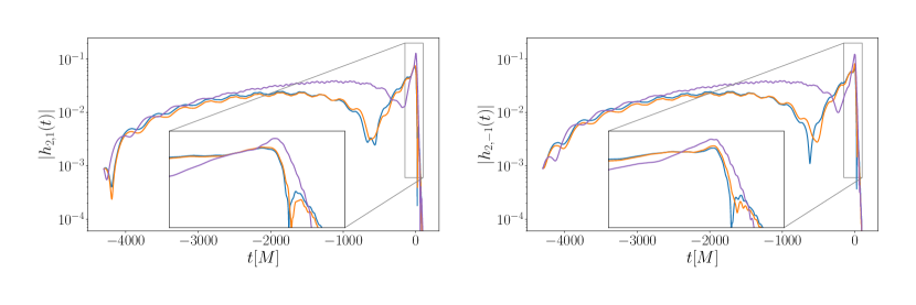
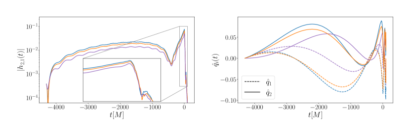
We first assess how well the vectorial effective spin parameter reproduces individual modes, in particular HMs, for different mass ratios. In Figure 1, we show the -modes for a fiducial precessing binary with and initial spins , . We find that (orange) captures the fully precessing modes (blue) significantly better than a simple parametrization (purple). In particular, we see that unlike , reproduces the amplitude and phasing of the mode oscillations on the orbital timescale and the amplitude modulations on the precession timescale much more faithfully. Additionally, amplitude modulations in the ringdown signal, which are completely missed in the -parametrization, are much better captured. We note that the precession of this fiducial binary is dominated by the secondary BH spin – a region in the spin parameter space where knowingly performs poorly. Additional examples are presented in Figs. LABEL:fig:EqualMassFiducial,_fig:q3Fiducial,_fig:FiducialSwitched in Appendix B, including a mass ratio binary with the precession dominated by the primary BH spin in Figure 15, where we still observe noticeable improvements with over .
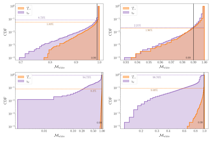
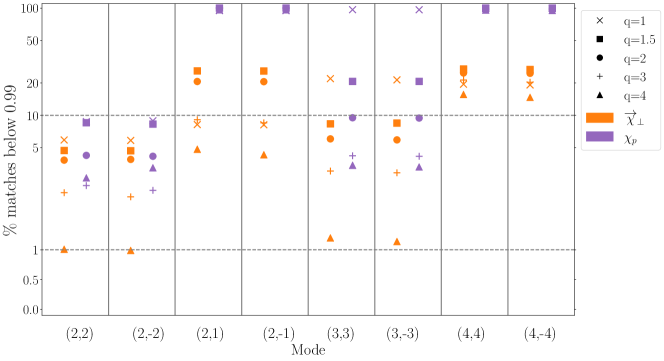
To quantify the efficacy of across the parameter space, we compute white noise mode-by-mode matches for the -modes and a selection of HMs for all binaries listed in the second column of Table 2. Figure 2 shows the cumulative match results for the and -modes for mass ratio and . Results for additional modes and mass ratios are shown in Figure 13 in Appendix A.
We expect the -parametrization to perform well at replicating the dominant -mode behavior, and indeed we see similar results in this mode for both parametrizations, if slightly improved with the new effective spin, except for the equal-mass case, where we find a more marked improvement. We attribute this to the fact that is designed to replicate the average precession rate, but in equal-mass configurations the in-plane spin vectors precess at the same rate and become orientationally locked, which is not captured correctly by Schmidt et al. (2015); Gerosa et al. (2021). Additionally, takes into account the in-plane spins on both black holes, while selects only the larger spin component leading to a systematic underestimation of the total in-plane spin for equal-mass cases.
We observe the most dramatic improvements in the modes. For example, for shown in Figure 2, the percentage of matches below decreases dramatically from with to with . Note that the long tails toward very low matches for the -parametrization, and the comparatively short ones of , are a generic feature across all HMs we analyzed, suggesting that better replicates the higher mode behavior even when it performs at its worst.
Intriguingly, for the and -modes, both parametrizations perform worst at , after which their performance improves with increasing mass ratio. To further investigate this intermediate region between the equal-mass regime and higher mass ratios where the secondary spin becomes less important, we performed additional white noise matches at mass ratios . We find that the performance of both spin mappings improves with increasing mass ratio for the and -modes, with consistently outperforming . We also find that performs worst around for the and -modes, but that the distributions for both mappings are fairly flat between and , and even at its worst still vastly outperforms . For example, in the -mode, at , the percentage of matches below is with , and only with . We also note that we find only minor differences between the positive and negative -modes for both mappings, and neither performs consistently worse at replicating either positive or negative -modes.
Additionally, our new mapping shows moderate improvements for the modes and striking improvements for the -modes, with the improvements particularly marked at equal-mass and at our highest mass ratio . In summary, we find that the -parametrization performs consistently better than for every mass ratio and across all modes, and in particular for odd -modes.
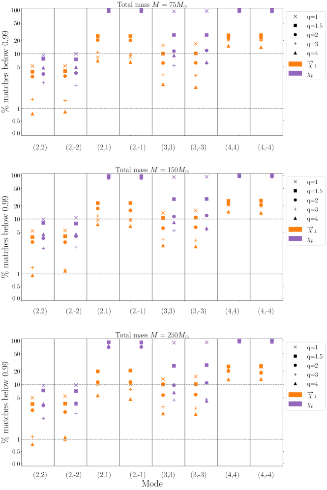
In addition to the white noise matches, we repeat the analysis using the projected O4 aLIGO PSD LIGO Scientific Collaboration and The Virgo Collaboration (2019) with Hz for three total masses compatible with the fixed length of the NR surrogate. For the PSD mode-by-mode matches, we obtain qualitatively similar results to the white noise matches as shown in Figure 13 in Appendix A. All of the matches improve slightly compared to the white noise matches across both mappings due to the frequency weighting of the PSD, but the features of our results and conclusions remain the same: The -mapping significantly improves upon for the - and -modes, with moderate improvements for the modes, and comparable if slightly better performance for the -modes.
IV.2 Strain analysis
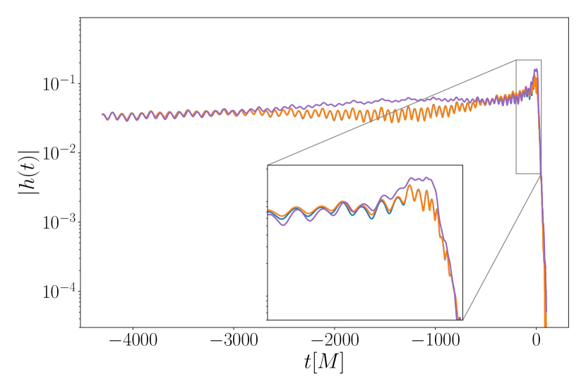
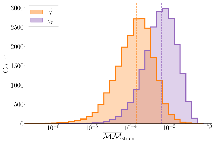
In the previous section we have demonstrated the improvement of over at the level of individual -modes. We now assess the degree to which the improvement in the HMs impacts the strain. Figure 3 shows the strain for the fiducial binary at an inclination of . The excellent agreement between the fully precessing waveform (blue) and the one parametrized by (orange) throughout the late inspiral as well as the merger ringdown is clearly visible. To quantify this agreement, we first compute the sky-and-polarization-averaged strain mismatches for 20,833 binary configurations as detailed in Table 2 using the O4 PSD and Hz. Our results for both effective parametrizations are shown in Figure 4. Using rather than , we find a median improvement of more than 1 order of magnitude from to . Furthermore, we note the non-negligible tail of extremely low mismatches below for .
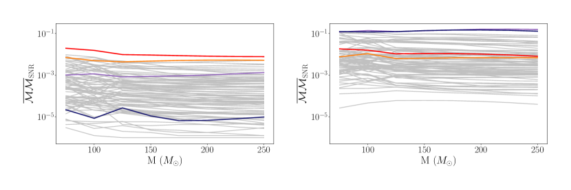
As low matches are often correlated with low SNRs and, therefore, with a lower detection probability, we also compute the SNR-weighted mismatch Eq. (22) for 100 randomly drawn intrinsic binary configurations as given in the fourth column of Table 2 for a moderate inclination of at . Similar to the sky-and-polarization-averaged strain mismatches, we see an improvement of around 1 order of magnitude when using the -parametrization instead of , as shown in Figure 5. The worst two cases for each parametrization are highlighted in both panels. We see that the worst cases for (red and orange) perform similarly under both mappings, if slightly better with the new -mapping. These cases both have a mass ratio of , which as noted previously in Sec. IV.1, is a mass ratio where both parametrizations perform worst. The worst cases for (purple and blue) on the other hand, show significant improvements of around 2 and 4 orders of magnitude respectively across the entire mass range when the -mapping is used.
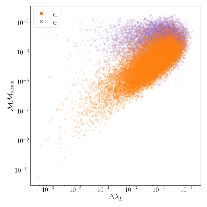
To better understand these marked improvements we employ several diagnostics. First, we investigate whether there exists a correlation between the initial opening angle of the precession cone [Eq. (1)] and the sky-and-polarization-averaged strain mismatch. We define the difference in the initial precession cone opening angle between the mapped and unmapped system, , as
| (23) |
where is given by Eq. (1). The definition of is the same as for , but replaces with , where is the initial total in-plane spin magnitude before the mapping and is the total in-plane spin magnitude after the mapping. All quantities are evaluated at the initial time , and we approximate by its Newtonian value , where is the reduced mass and with the orbital angular frequency.
Figure 6 shows against the strain mismatch for each of the 20,833 binaries, calculated with both the (orange) and (purple) effective spin mappings. For the new mapping, we see a clear correlation between lower values of and lower strain mismatches. Overall, the -parametrization yields a more accurate initial cone opening angle resulting in a more faithful representation of the fully precessing waveform.

The better agreement between the initial opening angles suggests that the spins themselves are captured more faithfully. To show this, as a second diagnostic we compare the spin evolutions of a fully precessing binary with its effective counterparts. Figure 7 shows the time evolution of the total in-plane spin (blue) for the fully precessing fiducial binary and those of the (orange) and (purple) parametrizations for the fiducial binary. We obtain these by transforming the spin evolutions in the inertial frame to the coprecessing frame using the quaternions. It is evident that the two-dimensional -mapping represents the full-spin dynamics much more faithfully than .
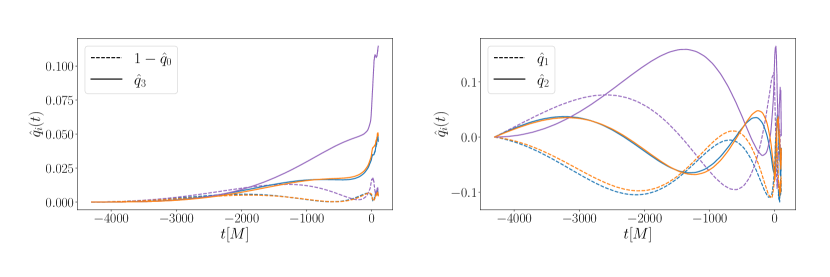
As a third diagnostic, we investigate how faithfully both mappings reproduce the fully spinning precession dynamics, which is represented by the unit quaternions . In Figure 8 we show the time evolution of the four unit quaternion components of the fiducial binary. The new effective spin mapping clearly replicates the time evolution of each quaternion component much more accurately than , with the most dramatic improvement observed for and .
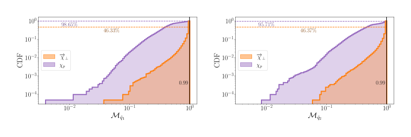
To quantify the improvement in replicating the precession dynamics, we perform a match calculation for each of the four quaternion components , , similar to the white match calculation in Eq. (14) but replacing the waveforms and with the quaternion components,
| (24) |
where we use , denotes the quaternion component from the fully precessing system, and is the quaternion component produced by the effective mapped system, with .
We compute the quaternion matches for the same 20,833 binaries used in the sky-and-polarization-averaged strain match calculations. Figure 9 shows the results for (left) and (right), which show the largest improvements: The percentage of matches below improves from with to with for , and for it improves from to . We see a negligible difference in the results for , which is well reproduced by both spin mappings: None of cases have a match value below . We see a small improvement in the results for , with the percentage of quaternion matches below dropping from for to for . These results indicate that the observed improvements when using can indeed be attributed to a more faithful representation of precession dynamics itself.
IV.3 Accuracy of the final spin and recoil
Finally, we quantify how well the -parametrization is able to reproduce the final spin and recoil of the remnant black hole. The final mass and spin of the remnant determine the quasinormal modes of the ringdown Press (1971); Chandrasekhar and Detweiler (1975); Detweiler (1980); Kokkotas and Schmidt (1999), so it is therefore crucial to understand the accuracy with which the final state can be replicated by the reduced set of spin parameters. We will focus on the final spin estimates as previous comparisons against NR simulations have shown that the final mass estimate is only very weakly dependent on precession Bohé et al. (2016).
To evaluate the final spin using the surrogate model we first evolve the BH spins in the inertial frame from to a time before merger, which are then used to evaluate the remnant fits of Ref. Varma et al. (2019b) via the public Python package surfinBH Varma and Stein (2018). The same procedure is followed to obtain the results under the two-spin parametrizations, where either effective spin map is applied at the initial time . We evaluate the remnant spin for the 20,833 binary configuration of column two in Table 2. We assess the accuracy of the final state under the two mappings by calculating the differences in the remnant spin magnitude , the final spin tilt angle , the azimuthal spin angle , the recoil velocity and its tilt angle defined as
| (25) | ||||
| (26) | ||||
| (27) | ||||
| (28) | ||||
| (29) |
where , and indicates the -components of the final spin vector in the inertial frame. We note that the remnant spin and recoil velocities are also returned in the inertial coordinate frame of the NR surrogate, which has no particular physical meaning postmerger. However, as we are computing relative differences in magnitudes and angles, this gauge choice has no effect on the results presented here.
We find marginal improvements in the accuracy of the final spin magnitude and tilt angle using the -mapping as opposed to . The median tilt angle difference improves slightly from rad with to rad with ; the absolute value also improves slightly from for to for . However, the largest improvement is found for the azimuthal angle , which encapsulates the difference in the relative angle in the -plane of the inertial frame as shown in Figure 10. We see a dramatic difference between the two mappings, with effectively reproducing the azimuthal orientation with a median error of less than rad, whereas the -mapping poorly replicates the azimuthal orientation with a median difference of more than 1 rad, and a significant proportion of differences around . We also note the significantly long tail of the histogram toward angle differences of zero.
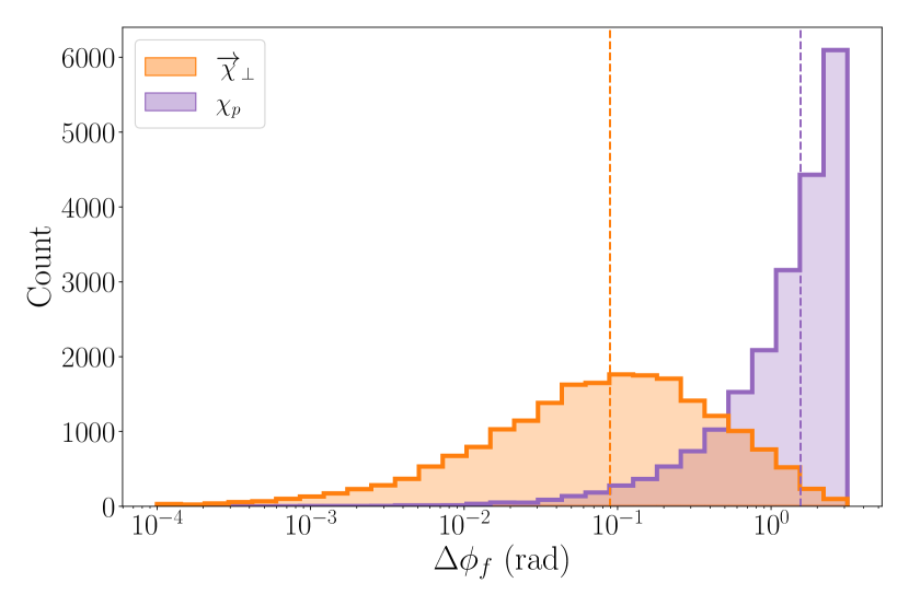
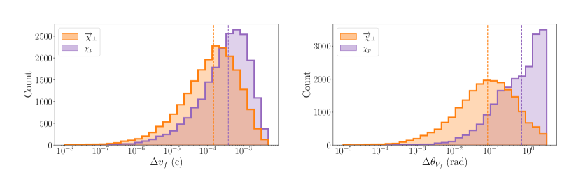
We now analyze the effect of the two mappings on the recoil velocity of the final black hole. For the recoil velocity tilt angle , i.e. the polar direction of the recoil, we find a large improvement from a median error of rad for to rad for as shown in the right panel of Figure 11. For the recoil velocity itself, we only find a modest improvement in from a median error of for to for , corresponding to an improvement in accuracy of km/s on average.
To summarize, overall the -parametrizations reproduce the final state, in particular the orientation of the final spin and the direction of the recoil, much more accurately. Both effective spin parametrizations perform similarly in determining the final spin magnitude.
We note that the comparison using is not directly comparable to the definition of the final spin used in semianalytical waveform models, which use (a variety of) in-plane spin corrections to modify the final spin of an aligned-spin binary Pratten et al. (2020a). The current generation of precessing Phenom models Hannam et al. (2014); Khan et al. (2020); Pratten et al. (2020b) apply a correction of the form , where is the remnant mass and is an effective in-plane spin contribution. In Hannam et al. (2014); Khan et al. (2020), is taken to be defined as in Eq. (3), which is similar to the results presented here obtained by applying the -mapping Bohé et al. (2016); Jiménez-Forteza et al. (2017). For the more recent model presented in Pratten et al. (2020a), a range of different final spin mappings have been implemented including the -mapping as well as a precession-averaged mapping that attempts to account for the change in the aligned-spin components due to nutation effects. The EOB models Ossokine et al. (2020) employ the final spin fits of Hofmann et al. (2016) which introduce corrections to the aligned-spin final state fits that depend on the angle between the two in-plane spin vectors and the projection of the spins along the orbital angular momentum. As discussed in Ossokine et al. (2020); Chandrasekhar and Detweiler (1975) and above, a crucial choice is the separation at which the spins are used to evaluate the final state, taken to be in Ossokine et al. (2020). This approach enables the effective-one-body models to account for the evolution of the spin vectors ensuring that the same waveform is produced irrespective of the initial separation.
V Discussion
The inclusion of fully relativistic precession effects in semianalytic IMR waveform models in the strong-field regime remains a challenging problem, with none of the current waveform models from either the Phenom or the EOB waveform family including calibration to NR in the precessing sector. The high dimensionality of the precessing BBH parameter space obfuscates a clear path for calibration. Effective spin parametrizations to reduce the number of spin degrees of freedom are a promising way forward to including fully relativistic precession in the strong-field regime. Previously, a scalar quantity was introduced to this effect but its efficacy was only demonstrated for the inspiral regime Schmidt et al. (2015). Here, we have assessed its applicability in the strong-field regime. Crucially, we have found that while does faithfully represent the -mode of the majority of fully precessing systems, it does not accurately reproduce HMs. Since HMs are excited by mass and spin asymmetries, which can be very pronounced for precessing binaries, they carry crucial parameter degeneracy breaking power Varma et al. (2014); Graff et al. (2015); Calderón Bustillo et al. (2016, 2017); Harry et al. (2018); Colleoni et al. (2020) making the accurate modeling of HMs critical. Therefore, NR calibration through a simple -parametrization is unlikely to be sufficient to satisfy the accuracy requirements for future GW observations.
To improve upon the shortcomings of , we have introduced a new two-dimensional effective precession spin vector, , and have performed extensive studies comparing the efficacy of to that of in the strong-field regime using the NR surrogate waveform model NRSur7dq4 Varma et al. (2019a). When analyzing individual -modes, in particular the -modes, we have found that performs significantly better than , but both effective parametrizations yield comparable results for the quadrupolar -modes. Correspondingly, we also have found a significant improvement in the precessing strain matches with the new mapping, from which we have concluded that the improved efficacy of over for the HMs has a significant effect on the accuracy of the overall strain, demonstrating the importance of accurately modeling HMs in precessing systems. Furthermore, we have found that performs better compared to in the equal-mass limit (see Figure 2). In this limit, the BH spins precess at the same rate, locked in orientation relative to each other. The parameter , which is defined to mimic the average rate of precession, performs knowingly poorly in this limit Schmidt et al. (2015); , on the other hand, is constructed such that it approximates the total in-plane spin of the fully precessing system at some reference time, leading to a significantly improved behavior in the equal-mass limit as anticipated from PN theory Apostolatos et al. (1994); Buonanno et al. (2004). As expected, we have found that performs increasingly better for larger mass ratios , where the spin on the smaller BH becomes negligible and hence the approximation with a single in-plane spin becomes more accurate. However, in the intermediate region between these two regimes, whilst still a considerable improvement upon , we have found a small drop in accuracy at a mass ratio of , where two-spin effects are important but are not fully captured in .
We have further demonstrated that the overall improvement relative to a -parametrization can be attributed to a more accurate replication of the precession dynamics itself when using the -parametrization. Indeed, in the case where only one of the two objects has nonzero in-plane spin components, the full dynamics are returned exactly, which is not the case for . The accurate capture of the precession dynamics of particular interest as a natural way for incorporating strong-field precession information into waveform models is through calibrating the precession dynamics itself, i.e. the rotation operator of Eq. (2) or, equivalently, the quaternions.
Additionally, we have also quantified how well the -mapping is able to replicate the final spin and recoil velocity of the remnant black hole. We have found a considerable improvement in the accuracy with which we have replicated the azimuthal direction of the remnant spin, and moderate improvements in the accuracy of the magnitude and direction of the recoil velocity. This suggests our -mapping is better able to replicate the final direction of GW emission, compared to . Previous work has demonstrated that the relative orientation of the in-plane spins at merger plays a crucial role in determining the final state properties Gonzalez et al. (2007); Bruegmann et al. (2008); Campanelli et al. (2007); Baker et al. (2008). We have attributed the observed improvements to the (partial) incorporation of two-spin effects, which are crucial for determining the recoil direction and velocity of the final BH.
Despite its significantly better performance in all areas, there are also caveats associated with : (i) For spin configurations with similar in-plane spin magnitudes, i.e. , we expect larger mismatches due to, by construction, the neglect of larger in-plane spin-spin couplings. (ii) We have normalized such that the Kerr limit is not violated. Consequently, for binaries with large spin magnitudes, will underestimate the magnitude of the in-plane spin in the system. Due to the limited spin parameter range of the surrogate, we have not been able to fully quantify the effect of this on the performance of the mapping. (iii) The conditional placement of on either of the two black holes introduces a discontinuity, in the sense that waveforms with placed on the primary BH show slightly different features from those with on the secondary BH. We note that all of our -mapped individual waveforms are physical and continuous, but that a shift in phenomenological features can occur between binary configurations with where is placed on the primary BH, against the same binary configuration with slightly smaller , where will be placed on the secondary BH. With this in mind, we have tested the performance of without the conditional placement. We have recalculated the sky-and-polarization-averaged strain matches shown in Figure 4 with always placed upon the primary BH irrespective of whether the precession is dominated by the primary or secondary BH, and indeed have found little difference from the original strain match distribution, with the median mismatch increasing minimally from to . Additionally, we have recalculated the white noise mode-by-mode matches of Eq. (14), again with always placed on the primary BH. While we have found little difference between the -mode results for with and without conditional placement, we have found that it has a marked effect on the results for HMs. For example, in the -mode at mass ratio , the percentage of mismatches below using without conditional placement rises to , compared to just if we include the conditional placement (under the -mapping the value is ). We therefore have concluded that for HMs, it is crucial to accurately capture spin asymmetries by placing the effective spin appropriately, to achieve an accurate mapped waveform mode.
Lastly, we have also tested whether the improvements found by using over are entirely due to the conditional placement, and whether an analogous conditional placement of would have similar effects. An example of imposing this condition also on is shown in Figure 16 in Appendix B for the fiducial binary, and we have indeed seen that the phenomenology is captured better. To quantify the improvement in the performance of when imposing conditional placement, we have recalculated the sky-and-polarization-averaged strain matches shown in Figure 4 with an analogous conditional placement for . We have found only a small improvement compared to the -mapping without conditional placement, with the median strain mismatch improving from to , compared to a median of with . We have also recalculated the mode-by-mode white noise matches shown in Figure 2, for both effective spin parametrizations, with and without conditional placement. These results are shown in Figure 17 in Appendix B. We see that for HMs at unequal-mass ratios, neither a conditionally placed , nor always placed on the primary object, can replicate the dramatic improvements we have previously seen in Figure 2. We therefore have surmised that the improvements we have seen in the performance of over are due to a combination of both the new parametrization itself, and the conditional placement, and that both are a necessary requirement to reproduce accurate precessing higher-order waveform modes.
Finally, we also note that the efficacy of has not been investigated for the special case of transitional precession, which leads to the tumbling of the total angular momentum when and . As with all effective mapping that neglects some spin contributions, however, we expect that the fine-tuned conditions needed for the occurrence of the transitional precession phase are not preserved under the mapping.
In conclusion, our results have demonstrated that by introducing the two-dimensional vector quantity , which partially accounts for two-spin effects, we can accurately reproduce the waveforms of fully precessing binaries, and in particular their HMs, in the strong-field regime across a wide range of the BBH parameter space. The effective reduction of four in-plane spin components to two provides a clear and tractable path forward to meaningfully incorporating precession effects in the strong-field regime into semianalytic waveform models with HMs, which we leave to future work.
Acknowledgments
We thank Serguei Ossokine, Sascha Husa, Davide Gerosa, Juan Calderón Bustillo, Matthew Mould, Daria Gangardt and our anonymous reviewer for useful discussions and comments. L. M. T. is supported by STFC, the School of Physics and Astronomy at the University of Birmingham and the Birmingham Institute for Gravitational Wave Astronomy. P. S. acknowledges the Dutch Research Council (NWO) Veni Grant No. 680-47-460. This manuscript has the LIGO document number P2000509.
Appendix A Complete Mode-by-Mode Match Results
Here we present the complete results of the white noise and O4 aLIGO PSD matches, for which a selection was presented in Figure 2. As described in Sec. III.3, we systematically sampled a total of intrinsic binary configurations , across the parameter range of the NR surrogate. For the PSD matches, which also require a total mass scale, we choose three masses compatible with the fixed length of the surrogate waveforms, bringing the total sampled binaries to . Full details of the sampling are given in Table 2.
The white match results are shown in Figure 12. We split the results by mass ratio and mode . We show the percentages of matches below between the fully spinning waveform, and the waveforms produced by each of the two effective spins, in orange, and in purple. We first note that at the match threshold of , we see an improvement by using over , across all mass ratios and modes. These improvements are particularly dramatic for higher modes, particularly the -modes. For example, at mass ratio , the percentage of -mode matches below using the parametrization is , which improves dramatically with to just . The parametrizations perform more similarly for the -modes, but even for the quadrupolar modes we see small improvements. For example, at mass ratio we see the percentage of -mode matches below improving from with to with .
Using the O4 aLIGO PSD, we similarly split the results by mass ratio and mode, and additionally by the total mass of the system. The results are shown in Figure 13. The PSD-weighted match results are qualitatively very similar to the white match results, albeit with small improvements across all matches due to the frequency weighting of the PSD, with only minor differences between each total mass.
Appendix B Additional Examples
Here we provide additional examples of waveform modes and corresponding precession dynamics produced using the effective spin mappings, both and . For each of the three binaries considered here, we show the -mode, as well as two of the four quaternion component evolutions. In all of the figures, the fully precessing system’s results are shown in blue, the results parameterized by in orange, and by in purple.
Our first example is an equal-mass binary, i.e. , with initial spins , . In this equal-mass limit, we expect to perform poorly, and to perform much better, as discussed more thoroughly in Sec. V. Indeed, in the left panel of Figure 14, we see that better replicates the -mode for this particular binary, with an amplitude closer to that of the fully precessing waveform and slightly improved phasing. We see the improvement by using as opposed to more clearly in the dynamics as shown in the right panel. The good agreement between the time evolution of fully precessing quaternion components in blue and those of the -mapped system in orange, is in stark contrast to the -mapped components in purple, which matches the dynamics poorly.
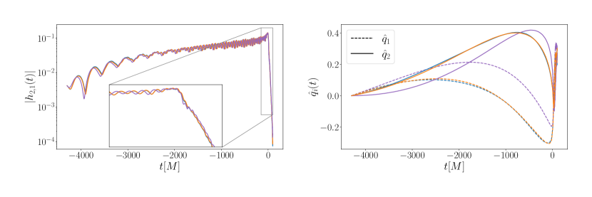
The second example is a binary with , and initial spins , . We note that in this example, unlike the fiducial binary shown in Figure 1, is mapped onto the primary BH. The left panel of Figure 15 shows the -mode, where we see that unlike in the previous example, the amplitudes of the two mapped waveform modes are very similar to that of the fully precessing mode (blue). However, clearly much better matches the phasing of the fully precessing mode, with the orange and blue lines being indistinguishable for much of the inspiral, in contrast to which shows a clear dephasing, especially in the merger ringdown. We also see that, like for the other fiducial binaries, the quaternion components mapped by , much more faithfully represent the fully precessing quaternions, compared to the -mapped components, demonstrating that better replicates the precession dynamics of the fully precessing system.
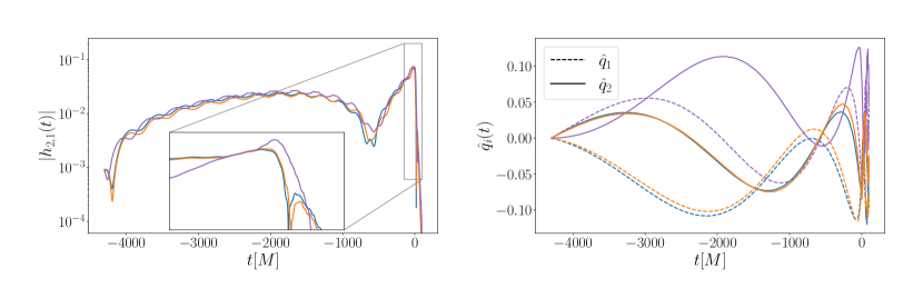
Third, we illustrate the impact of the conditional placement using the original fiducial binary of Figure 1, but this time showing the effect of an analogous conditional placement with the -parametrization. In Figure 16, we show the fully precessing fiducial binary in blue, -mapped system in orange, and the -mapped system with conditional placement in purple. We note that now both and are placed on the secondary BH for this binary. We can see in the left panel that the conditional placement does improve the accuracy with which reproduces the -mode; however the -mapping still reproduces the phasing of the mode significantly better. Additionally, we see in the right panel that the conditional placement of does not produce the precession dynamics more accurately, with still much more closely matching the time evolution of the fully precessing quaternion components.
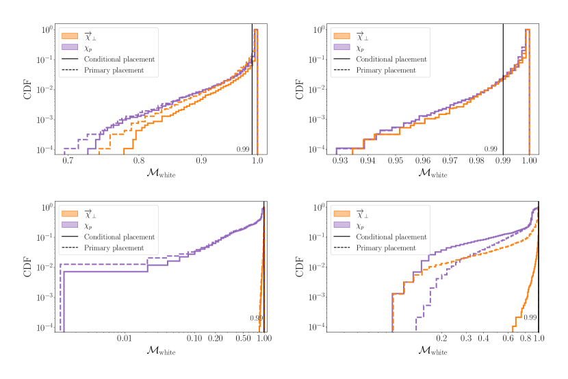
In addition to these individual cases, in Figure 17 we recalculate the white noise mode-by-mode matches shown in Figure 2, for both spin parametrizations and , using (i) conditional placement (solid) and (ii) placement always on the primary black hole (dashed). We note that in all four panels, the best performance is obtained when conditionally placing . The (2,2)-mode at mass ratio (top left) shows a small improvement in both parametrizations’ performance when conditional placement is included. The biggest improvement can be seen in the (2,1)-mode at mass ratio (bottom right), where a conditionally placed dramatically outperforms all other configurations, and neither a conditionally placed , nor a affixed to the primary would be able to achieve these improvements. Interestingly, this panel also displays the only instance where conditional placement can worsen the performance of . Therefore, we conclude that particularly for HMs at unequal-mass ratios, to obtain the dramatic improvements we have seen, both the new effective spin and conditional placement are required.
References
- Abbott et al. (2016a) B.P. Abbott et al. (LIGO Scientific, Virgo), “Observation of Gravitational Waves from a Binary Black Hole Merger,” Phys. Rev. Lett. 116, 061102 (2016a), arXiv:1602.03837 [gr-qc] .
- Abbott et al. (2018) B.P. Abbott et al. (KAGRA, LIGO Scientific, VIRGO), “Prospects for Observing and Localizing Gravitational-Wave Transients with Advanced LIGO, Advanced Virgo and KAGRA,” Living Rev. Rel. 21, 3 (2018), arXiv:1304.0670 [gr-qc] .
- Tse et al. (2019) M. Tse et al., “Quantum-Enhanced Advanced LIGO Detectors in the Era of Gravitational-Wave Astronomy,” Phys. Rev. Lett. 123, 231107 (2019).
- Acernese et al. (2015) F. Acernese et al. (VIRGO), “Advanced Virgo: a second-generation interferometric gravitational wave detector,” Class. Quant. Grav. 32, 024001 (2015), arXiv:1408.3978 [gr-qc] .
- Acernese et al. (2019) F. Acernese et al. (Virgo), “Increasing the Astrophysical Reach of the Advanced Virgo Detector via the Application of Squeezed Vacuum States of Light,” Phys. Rev. Lett. 123, 231108 (2019).
- Abbott et al. (2019) B.P. Abbott et al. (LIGO Scientific, Virgo), “GWTC-1: A Gravitational-Wave Transient Catalog of Compact Binary Mergers Observed by LIGO and Virgo during the First and Second Observing Runs,” Phys. Rev. X 9, 031040 (2019), arXiv:1811.12907 [astro-ph.HE] .
- Abbott et al. (2020a) R. Abbott et al. (LIGO Scientific, Virgo), “GWTC-2: Compact Binary Coalescences Observed by LIGO and Virgo During the First Half of the Third Observing Run,” (2020a), arXiv:2010.14527 [gr-qc] .
- Abbott et al. (2017a) B.P. Abbott et al. (LIGO Scientific, Virgo), “GW170817: Observation of Gravitational Waves from a Binary Neutron Star Inspiral,” Phys. Rev. Lett. 119, 161101 (2017a), arXiv:1710.05832 [gr-qc] .
- Abbott et al. (2017b) B.P. Abbott et al. (LIGO Scientific, Virgo, Fermi GBM, INTEGRAL, IceCube, AstroSat Cadmium Zinc Telluride Imager Team, IPN, Insight-Hxmt, ANTARES, Swift, AGILE Team, 1M2H Team, Dark Energy Camera GW-EM, DES, DLT40, GRAWITA, Fermi-LAT, ATCA, ASKAP, Las Cumbres Observatory Group, OzGrav, DWF (Deeper Wider Faster Program), AST3, CAASTRO, VINROUGE, MASTER, J-GEM, GROWTH, JAGWAR, CaltechNRAO, TTU-NRAO, NuSTAR, Pan-STARRS, MAXI Team, TZAC Consortium, KU, Nordic Optical Telescope, ePESSTO, GROND, Texas Tech University, SALT Group, TOROS, BOOTES, MWA, CALET, IKI-GW Follow-up, H.E.S.S., LOFAR, LWA, HAWC, Pierre Auger, ALMA, Euro VLBI Team, Pi of Sky, Chandra Team at McGill University, DFN, ATLAS Telescopes, High Time Resolution Universe Survey, RIMAS, RATIR, SKA South Africa/MeerKAT), “Multi-messenger Observations of a Binary Neutron Star Merger,” Astrophys. J. Lett. 848, L12 (2017b), arXiv:1710.05833 [astro-ph.HE] .
- Abbott et al. (2020b) R. Abbott et al. (LIGO Scientific, Virgo), “GW190521: A Binary Black Hole Merger with a Total Mass of ,” Phys. Rev. Lett. 125, 101102 (2020b), arXiv:2009.01075 [gr-qc] .
- Abbott et al. (2020c) R. Abbott et al. (LIGO Scientific, Virgo), “Properties and Astrophysical Implications of the 150 M⊙ Binary Black Hole Merger GW190521,” Astrophys. J. Lett. 900, L13 (2020c), arXiv:2009.01190 [astro-ph.HE] .
- Abbott et al. (2020d) R. Abbott et al. (LIGO Scientific, Virgo), “GW190412: Observation of a Binary-Black-Hole Coalescence with Asymmetric Masses,” Phys. Rev. D 102, 043015 (2020d), arXiv:2004.08342 [astro-ph.HE] .
- Abbott et al. (2020e) R. Abbott et al. (LIGO Scientific, Virgo), “GW190814: Gravitational Waves from the Coalescence of a 23 Solar Mass Black Hole with a 2.6 Solar Mass Compact Object,” Astrophys. J. Lett. 896, L44 (2020e), arXiv:2006.12611 [astro-ph.HE] .
- Nitz et al. (2019) Alexander H. Nitz, Thomas Dent, Gareth S. Davies, Sumit Kumar, Collin D. Capano, Ian Harry, Simone Mozzon, Laura Nuttall, Andrew Lundgren, and Márton Tápai, “2-OGC: Open Gravitational-wave Catalog of binary mergers from analysis of public Advanced LIGO and Virgo data,” Astrophys. J. 891, 123 (2019), arXiv:1910.05331 [astro-ph.HE] .
- Venumadhav et al. (2020) Tejaswi Venumadhav, Barak Zackay, Javier Roulet, Liang Dai, and Matias Zaldarriaga, “New binary black hole mergers in the second observing run of Advanced LIGO and Advanced Virgo,” Phys. Rev. D 101, 083030 (2020), arXiv:1904.07214 [astro-ph.HE] .
- Hannam et al. (2014) Mark Hannam, Patricia Schmidt, Alejandro Bohé, Leïla Haegel, Sascha Husa, Frank Ohme, Geraint Pratten, and Michael Pürrer, “Simple Model of Complete Precessing Black-Hole-Binary Gravitational Waveforms,” Phys. Rev. Lett. 113, 151101 (2014), arXiv:1308.3271 [gr-qc] .
- Pan et al. (2014) Yi Pan, Alessandra Buonanno, Andrea Taracchini, Lawrence E. Kidder, Abdul H. Mroué, Harald P. Pfeiffer, Mark A. Scheel, and Béla Szilágyi, “Inspiral-merger-ringdown waveforms of spinning, precessing black-hole binaries in the effective-one-body formalism,” Phys. Rev. D 89, 084006 (2014), arXiv:1307.6232 [gr-qc] .
- Khan et al. (2020) Sebastian Khan, Frank Ohme, Katerina Chatziioannou, and Mark Hannam, “Including higher order multipoles in gravitational-wave models for precessing binary black holes,” Phys. Rev. D 101, 024056 (2020), arXiv:1911.06050 [gr-qc] .
- Pratten et al. (2020a) Geraint Pratten et al., “Let’s twist again: computationally efficient models for the dominant and sub-dominant harmonic modes of precessing binary black holes,” (2020a), arXiv:2004.06503 [gr-qc] .
- Ossokine et al. (2020) Serguei Ossokine et al., “Multipolar Effective-One-Body Waveforms for Precessing Binary Black Holes: Construction and Validation,” Phys. Rev. D 102, 044055 (2020), arXiv:2004.09442 [gr-qc] .
- Reitze et al. (2019) David Reitze et al., “Cosmic Explorer: The U.S. Contribution to Gravitational-Wave Astronomy beyond LIGO,” Bull. Am. Astron. Soc. 51, 035 (2019), arXiv:1907.04833 [astro-ph.IM] .
- Maggiore et al. (2020) Michele Maggiore et al., “Science Case for the Einstein Telescope,” JCAP 03, 050 (2020), arXiv:1912.02622 [astro-ph.CO] .
- Abbott et al. (2017c) Benjamin P Abbott et al. (LIGO Scientific), “Exploring the Sensitivity of Next Generation Gravitational Wave Detectors,” Class. Quant. Grav. 34, 044001 (2017c), arXiv:1607.08697 [astro-ph.IM] .
- Pürrer and Haster (2020) Michael Pürrer and Carl-Johan Haster, “Gravitational waveform accuracy requirements for future ground-based detectors,” Phys. Rev. Res. 2, 023151 (2020), arXiv:1912.10055 [gr-qc] .
- Buonanno and Damour (1999) A. Buonanno and T. Damour, “Effective one-body approach to general relativistic two-body dynamics,” Phys. Rev. D 59, 084006 (1999), arXiv:gr-qc/9811091 [gr-qc] .
- Ajith et al. (2011) P. Ajith et al., “Inspiral-merger-ringdown waveforms for black-hole binaries with non-precessing spins,” Phys. Rev. Lett. 106, 241101 (2011), arXiv:0909.2867 [gr-qc] .
- Santamaria et al. (2010) L. Santamaria et al., “Matching post-Newtonian and numerical relativity waveforms: systematic errors and a new phenomenological model for non-precessing black hole binaries,” Phys. Rev. D 82, 064016 (2010), arXiv:1005.3306 [gr-qc] .
- Blackman et al. (2017a) Jonathan Blackman, Scott E. Field, Mark A. Scheel, Chad R. Galley, Daniel A. Hemberger, Patricia Schmidt, and Rory Smith, “A Surrogate Model of Gravitational Waveforms from Numerical Relativity Simulations of Precessing Binary Black Hole Mergers,” Phys. Rev. D 95, 104023 (2017a), arXiv:1701.00550 [gr-qc] .
- Blackman et al. (2017b) Jonathan Blackman, Scott E. Field, Mark A. Scheel, Chad R. Galley, Christian D. Ott, Michael Boyle, Lawrence E. Kidder, Harald P. Pfeiffer, and Béla Szilágyi, “Numerical relativity waveform surrogate model for generically precessing binary black hole mergers,” Phys. Rev. D 96, 024058 (2017b), arXiv:1705.07089 [gr-qc] .
- Ramos-Buades et al. (2020) Antoni Ramos-Buades, Patricia Schmidt, Geraint Pratten, and Sascha Husa, “Validity of common modeling approximations for precessing binary black holes with higher-order modes,” Phys. Rev. D 101, 103014 (2020), arXiv:2001.10936 [gr-qc] .
- Apostolatos et al. (1994) Theocharis A. Apostolatos, Curt Cutler, Gerald J. Sussman, and Kip S. Thorne, “Spin induced orbital precession and its modulation of the gravitational wave forms from merging binaries,” Phys. Rev. D 49, 6274–6297 (1994).
- Kidder (1995) Lawrence E. Kidder, “Coalescing binary systems of compact objects to postNewtonian 5/2 order. 5. Spin effects,” Phys. Rev. D 52, 821–847 (1995), arXiv:gr-qc/9506022 .
- Vecchio (2004) Alberto Vecchio, “LISA observations of rapidly spinning massive black hole binary systems,” Phys. Rev. D 70, 042001 (2004), arXiv:astro-ph/0304051 .
- van der Sluys et al. (2008) M.V. van der Sluys, C. Röver, A. Stroeer, V. Raymond, I. Mandel, N. Christensen, V. Kalogera, R. Meyer, and A. Vecchio, “Gravitational-Wave Astronomy with Inspiral Signals of Spinning Compact-Object Binaries,” Astrophys. J. Lett. 688, L61 (2008), arXiv:0710.1897 [astro-ph] .
- Lang and Hughes (2006) Ryan N. Lang and Scott A. Hughes, “Measuring coalescing massive binary black holes with gravitational waves: The Impact of spin-induced precession,” Phys. Rev. D 74, 122001 (2006), [Erratum: Phys.Rev.D 75, 089902 (2007), Erratum: Phys.Rev.D 77, 109901 (2008)], arXiv:gr-qc/0608062 .
- Cho et al. (2013) Hee-Suk Cho, Evan Ochsner, Richard O’Shaughnessy, Chunglee Kim, and Chang-Hwan Lee, “Gravitational waves from black hole-neutron star binaries: Effective Fisher matrices and parameter estimation using higher harmonics,” Phys. Rev. D 87, 024004 (2013), arXiv:1209.4494 [gr-qc] .
- O’Shaughnessy et al. (2014) R. O’Shaughnessy, Benjamin Farr, E. Ochsner, Hee-Suk Cho, V. Raymond, Chunglee Kim, and Chang-Hwan Lee, “Parameter estimation of gravitational waves from precessing black hole-neutron star inspirals with higher harmonics,” Phys. Rev. D 89, 102005 (2014), arXiv:1403.0544 [gr-qc] .
- Chatziioannou et al. (2015) Katerina Chatziioannou, Neil Cornish, Antoine Klein, and Nicolas Yunes, “Spin-Precession: Breaking the Black Hole–Neutron Star Degeneracy,” Astrophys. J. Lett. 798, L17 (2015), arXiv:1402.3581 [gr-qc] .
- Pratten et al. (2020b) Geraint Pratten, Patricia Schmidt, Riccardo Buscicchio, and Lucy M. Thomas, “Measuring precession in asymmetric compact binaries,” Phys. Rev. Res. 2, 043096 (2020b), arXiv:2006.16153 [gr-qc] .
- Schmidt et al. (2011) Patricia Schmidt, Mark Hannam, Sascha Husa, and P. Ajith, “Tracking the precession of compact binaries from their gravitational-wave signal,” Phys. Rev. D 84, 024046 (2011), arXiv:1012.2879 [gr-qc] .
- Schmidt et al. (2012) Patricia Schmidt, Mark Hannam, and Sascha Husa, “Towards models of gravitational waveforms from generic binaries: A simple approximate mapping between precessing and non-precessing inspiral signals,” Phys. Rev. D 86, 104063 (2012), arXiv:1207.3088 [gr-qc] .
- Schmidt et al. (2015) Patricia Schmidt, Frank Ohme, and Mark Hannam, “Towards models of gravitational waveforms from generic binaries II: Modelling precession effects with a single effective precession parameter,” Phys. Rev. D 91, 024043 (2015), arXiv:1408.1810 [gr-qc] .
- Kesden et al. (2015) Michael Kesden, Davide Gerosa, Richard O’Shaughnessy, Emanuele Berti, and Ulrich Sperhake, “Effective potentials and morphological transitions for binary black-hole spin precession,” Phys. Rev. Lett. 114, 081103 (2015), arXiv:1411.0674 [gr-qc] .
- Gerosa et al. (2015) Davide Gerosa, Michael Kesden, Ulrich Sperhake, Emanuele Berti, and Richard O’Shaughnessy, “Multi-timescale analysis of phase transitions in precessing black-hole binaries,” Phys. Rev. D 92, 064016 (2015), arXiv:1506.03492 [gr-qc] .
- Pekowsky et al. (2013) L. Pekowsky, R. O’Shaughnessy, J. Healy, and D. Shoemaker, “Comparing gravitational waves from nonprecessing and precessing black hole binaries in the corotating frame,” Phys. Rev. D 88, 024040 (2013), arXiv:1304.3176 [gr-qc] .
- Gerosa et al. (2021) Davide Gerosa, Matthew Mould, Daria Gangardt, Patricia Schmidt, Geraint Pratten, and Lucy M. Thomas, “A generalized precession parameter to interpret gravitational-wave data,” Phys. Rev. D 103, 064067 (2021), arXiv:2011.11948 [gr-qc] .
- Akcay et al. (2020) Sarp Akcay, Rossella Gamba, and Sebastiano Bernuzzi, “A hybrid post-Newtonian – effective-one-body scheme for spin-precessing compact-binary waveforms,” (2020), arXiv:2005.05338 [gr-qc] .
- Abbott et al. (2016b) B.P. Abbott et al. (LIGO Scientific, Virgo), “Properties of the Binary Black Hole Merger GW150914,” Phys. Rev. Lett. 116, 241102 (2016b), arXiv:1602.03840 [gr-qc] .
- Varma et al. (2019a) Vijay Varma, Scott E. Field, Mark A. Scheel, Jonathan Blackman, Davide Gerosa, Leo C. Stein, Lawrence E. Kidder, and Harald P. Pfeiffer, “Surrogate models for precessing binary black hole simulations with unequal masses,” Phys. Rev. Research. 1, 033015 (2019a), arXiv:1905.09300 [gr-qc] .
- (50) Jonathan Blackman, Scott E. Field, Chad R. Galley, and Vijay Varma, “gwsurrogate,” https://pypi.python.org/pypi/gwsurrogate/.
- Field et al. (2014) Scott E. Field, Chad R. Galley, Jan S. Hesthaven, Jason Kaye, and Manuel Tiglio, “Fast prediction and evaluation of gravitational waveforms using surrogate models,” Phys. Rev. X 4, 031006 (2014), arXiv:1308.3565 [gr-qc] .
- Blackman et al. (2015) Jonathan Blackman, Scott E. Field, Chad R. Galley, Béla Szilágyi, Mark A. Scheel, Manuel Tiglio, and Daniel A. Hemberger, “Fast and Accurate Prediction of Numerical Relativity Waveforms from Binary Black Hole Coalescences Using Surrogate Models,” Phys. Rev. Lett. 115, 121102 (2015), arXiv:1502.07758 [gr-qc] .
- Boyle (2013) Michael Boyle, “Angular velocity of gravitational radiation from precessing binaries and the corotating frame,” Phys. Rev. D 87, 104006 (2013), arXiv:1302.2919 [gr-qc] .
- LIGO Scientific Collaboration and The Virgo Collaboration (2019) LIGO Scientific Collaboration and The Virgo Collaboration, “Noise curves used for Simulations in the update of the Observing Scenarios Paper,” https://dcc.ligo.org/LIGO-T2000012/public (2019).
- Capano et al. (2014) Collin Capano, Yi Pan, and Alessandra Buonanno, “Impact of higher harmonics in searching for gravitational waves from nonspinning binary black holes,” Phys. Rev. D 89, 102003 (2014), arXiv:1311.1286 [gr-qc] .
- Babak et al. (2017) Stanislav Babak, Andrea Taracchini, and Alessandra Buonanno, “Validating the effective-one-body model of spinning, precessing binary black holes against numerical relativity,” Phys. Rev. D 95, 024010 (2017), arXiv:1607.05661 [gr-qc] .
- Press (1971) William H. Press, “Long Wave Trains of Gravitational Waves from a Vibrating Black Hole,” Astrophys. J. Lett. 170, L105–L108 (1971).
- Chandrasekhar and Detweiler (1975) S. Chandrasekhar and Steven L. Detweiler, “The quasi-normal modes of the Schwarzschild black hole,” Proc. Roy. Soc. Lond. A 344, 441–452 (1975).
- Detweiler (1980) Steven L. Detweiler, “Black holes and gravitational waves. III. The resonant frequencies of rotating holes,” Astrophys. J. 239, 292–295 (1980).
- Kokkotas and Schmidt (1999) Kostas D. Kokkotas and Bernd G. Schmidt, “Quasinormal modes of stars and black holes,” Living Rev. Rel. 2, 2 (1999), arXiv:gr-qc/9909058 .
- Bohé et al. (2016) Alejandro Bohé, Mark Hannam, Sascha Husa, Frank Ohme, Michael Pürrer, and Patricia. Schmidt, “PhenomPv2 – technical notes for the LAL implementation,” https://dcc.ligo.org/LIGO-T1500602/public (2016).
- Varma et al. (2019b) Vijay Varma, Davide Gerosa, Leo C. Stein, François Hébert, and Hao Zhang, “High-accuracy mass, spin, and recoil predictions of generic black-hole merger remnants,” Phys. Rev. Lett. 122, 011101 (2019b), arXiv:1809.09125 [gr-qc] .
- Varma and Stein (2018) Vijay Varma and Leo C. Stein, “vijayvarma392/surfinBH: Surrogate Final BH properties,” (2018).
- Jiménez-Forteza et al. (2017) Xisco Jiménez-Forteza, David Keitel, Sascha Husa, Mark Hannam, Sebastian Khan, and Michael Pürrer, “Hierarchical data-driven approach to fitting numerical relativity data for nonprecessing binary black holes with an application to final spin and radiated energy,” Phys. Rev. D 95, 064024 (2017), arXiv:1611.00332 [gr-qc] .
- Hofmann et al. (2016) Fabian Hofmann, Enrico Barausse, and Luciano Rezzolla, “The final spin from binary black holes in quasi-circular orbits,” Astrophys. J. Lett. 825, L19 (2016), arXiv:1605.01938 [gr-qc] .
- Varma et al. (2014) Vijay Varma, Parameswaran Ajith, Sascha Husa, Juan Calderon Bustillo, Mark Hannam, and Michael Pürrer, “Gravitational-wave observations of binary black holes: Effect of nonquadrupole modes,” Phys. Rev. D 90, 124004 (2014), arXiv:1409.2349 [gr-qc] .
- Graff et al. (2015) Philip B. Graff, Alessandra Buonanno, and B. S. Sathyaprakash, “Missing Link: Bayesian detection and measurement of intermediate-mass black-hole binaries,” Phys. Rev. D 92, 022002 (2015), arXiv:1504.04766 [gr-qc] .
- Calderón Bustillo et al. (2016) Juan Calderón Bustillo, Sascha Husa, Alicia M. Sintes, and Michael Pürrer, “Impact of gravitational radiation higher order modes on single aligned-spin gravitational wave searches for binary black holes,” Phys. Rev. D 93, 084019 (2016), arXiv:1511.02060 [gr-qc] .
- Calderón Bustillo et al. (2017) Juan Calderón Bustillo, Pablo Laguna, and Deirdre Shoemaker, “Detectability of gravitational waves from binary black holes: Impact of precession and higher modes,” Phys. Rev. D 95, 104038 (2017), arXiv:1612.02340 [gr-qc] .
- Harry et al. (2018) Ian Harry, Juan Calderón Bustillo, and Alex Nitz, “Searching for the full symphony of black hole binary mergers,” Phys. Rev. D 97, 023004 (2018), arXiv:1709.09181 [gr-qc] .
- Colleoni et al. (2020) Marta Colleoni, Maite Mateu-Lucena, Héctor Estellés, Cecilio García-Quirós, David Keitel, Geraint Pratten, Antoni Ramos-Buades, and Sascha Husa, “Towards the routine use of subdominant harmonics in gravitational-wave inference: re-analysis of GW190412 with generation X waveform models,” (2020), arXiv:2010.05830 [gr-qc] .
- Buonanno et al. (2004) Alessandra Buonanno, Yan-bei Chen, Yi Pan, and Michele Vallisneri, “A Quasi-physical family of gravity-wave templates for precessing binaries of spinning compact objects. 2. Application to double-spin precessing binaries,” Phys. Rev. D 70, 104003 (2004), [Erratum: Phys.Rev.D 74, 029902 (2006)], arXiv:gr-qc/0405090 .
- Gonzalez et al. (2007) Jose A. Gonzalez, Ulrich Sperhake, Bernd Bruegmann, Mark Hannam, and Sascha Husa, “Total recoil: The Maximum kick from nonspinning black-hole binary inspiral,” Phys. Rev. Lett. 98, 091101 (2007), arXiv:gr-qc/0610154 .
- Bruegmann et al. (2008) Bernd Bruegmann, Jose A. Gonzalez, Mark Hannam, Sascha Husa, and Ulrich Sperhake, “Exploring black hole superkicks,” Phys. Rev. D 77, 124047 (2008), arXiv:0707.0135 [gr-qc] .
- Campanelli et al. (2007) Manuela Campanelli, Carlos O. Lousto, Yosef Zlochower, and David Merritt, “Maximum gravitational recoil,” Phys. Rev. Lett. 98, 231102 (2007), arXiv:gr-qc/0702133 .
- Baker et al. (2008) John G. Baker, William D. Boggs, Joan Centrella, Bernard J. Kelly, Sean T. McWilliams, M.Coleman Miller, and James R. van Meter, “Modeling kicks from the merger of generic black-hole binaries,” Astrophys. J. Lett. 682, L29–L32 (2008), arXiv:0802.0416 [astro-ph] .