Recursive Tree Grammar Autoencoders

Abstract

Machine learning on trees has been mostly focused on trees as input to algorithms. Much less research has investigated trees as output, which has many applications, such as molecule optimization for drug discovery, or hint generation for intelligent tutoring systems. In this work, we propose a novel autoencoder approach, called recursive tree grammar autoencoder (RTG-AE), which encodes trees via a bottom-up parser and decodes trees via a tree grammar, both learned via recursive neural networks that minimize the variational autoencoder loss. The resulting encoder and decoder can then be utilized in subsequent tasks, such as optimization and time series prediction. RTG-AEs are the first model to combine variational autoencoders, grammatical knowledge, and recursive processing. Our key message is that this unique combination of all three elements outperforms models which combine any two of the three. In particular, we perform an ablation study to show that our proposed method improves the autoencoding error, training time, and optimization score on synthetic as well as real datasets compared to four baselines.

Keywords: Recursive Neural Networks, Tree Grammars, Representation Learning, Variational Autoencoders

1 Introduction

Deep neural networks on trees have made significant progress in recent years with novel models that achieved unprecedented performance on tree-related tasks, such as tree echo state networks (Gallicchio and Micheli, 2013), tree LSTMs (Tai et al., 2015), code2vec (Alon et al., 2019), or models from the graph neural network family (Kipf and Welling, 2017; Micheli, 2009; Scarselli et al., 2009). However, these advancements are mostly limited to tasks with numeric output, such as classification and regression. By contrast, much less research has focused on tasks that require trees as output, such as as molecular design (Kusner et al., 2017; Jin et al., 2018) or hint generation in intelligent tutoring systems (Paaßen et al., 2018). In this work, we propose a novel autoencoding model which can encode a tree $\hat{x}$ into a vector encoding $\vec{z}$ and decode a vector $\vec{z}$ back into a tree $\hat{x}$. Thus, our model supports not only classification and regression tasks but also optimization over trees or time series prediction on trees.

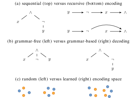
There are three key roots for our approach in prior literature. First, Kusner et al. (2017) represented strings as a sequence of context-free grammar rules, encoded this rule sequence in the latent space of a variational autoencoder using a convolutional neural net, and decoded back into a rule sequence with a gated recurrent unit (GRU) (Cho et al., 2014). We believe that, for trees, the sequential processing proposed by Kusner et al. (2017) is insufficient because it introduces long-range dependencies. For example, when processing the tree $\wedge(x,\neg(y))$, a sequential representation would be $y,\neg,x,\wedge$. When processing $\wedge$, we want to take the information from its children $x$ and $\neg$ into account, but $\neg$ is already two steps away. If we replace $x$ with a large subtree, this distance can become arbitrarily large. To avoid such long-range dependencies, we propose recursive processing, where the information flow follows the structure of the tree (Figure 1, a) (Tai et al., 2015; Pollack, 1990; Sperduti and Starita, 1997). Therefore, we call our approach recursive tree grammar autoencoders (RTG-AEs).

Second, Zhang et al. (2019b) suggested a variational autoencoder for graphs by representing a graph as a sequence of node and edge insertions, which in turn can be encoded and decoded with a recurrent neural network. While this approach is directly applicable to trees, it needs to learn all grammatical structure of a domain, in particular the appropriate number and order of children in each context. This can lead to obvious errors, such as decoding the tree $\wedge(x,\neg(y))$ as $\wedge(x,\neg,y)$, which is clearly ungrammatical (Figure 1, b). Instead, in line with Kusner et al. (2017), we believe that grammatical knowledge is crucial as an inductive bias to prevent easily avoidable decoding mistakes. In contrast to Kusner et al. (2017), we employ tree grammars instead of string grammars.

Finally, in our own previous work (Paaßen et al., 2020), we implemented a recursive tree grammar neural network architecture using tree echo state networks (Gallicchio and Micheli, 2013). This shallow learning approach utilizes a random, high-dimensional and scattered encoding space. In this work, we propose to learn the entire autoencoder end-to-end via a variational autoencoding approach, thus yielding a lower-dimensional, smoother encoding space in which sampling and optimization is easier (Figure 1, c).

Figure 1: An illustration of the advantages (a) of recursive over sequential processing, (b) of utilizing grammatical knowledge, and (c) of learning the encoding end-to-end. In c), each point represents the encoding of a tree and color indicates some semantic attribute with respect to which the encoding space should be smooth (right).

As such, RTG-AEs combine variational autoencoders, grammatical knowledge, and recursive processing. Our key message is that this combination outperforms approaches which combine only two of these three aspects. In particular, we compare to the model of Kusner et al. (2017) and to an ablated version of RTG-AE which combine variational autoencoding with grammatical knowledge but process the trees sequentially; we compare to the DVAE of Zhang et al. (2019b) which combines variational autoencoding with recursive processing but does not use grammatical knowledge; and we compare to TES-AE (Paaßen et al., 2020), which is an ablated version of RTG-AE that combines grammatical knowledge with recursive processing but only trains the decoding layers, while we propose end-to-end learning. We evaluate RTG-AEs and all baselines on four data sets, including two synthetic and two real-world ones, including hyperparameter optimization and crossvalidation to give more robust performance estimates compared to prior work. We also run optimization with multiple repeats to provide more robust results. Additionally, our paper contributes a correctness proof of our encoding based on the theory of regular tree grammars.

We begin by discussing background and related work before we introduce the RTG-AE architecture and evaluate it on four datasets, including two synthetic and two real-world ones.

2 Background and Related Work

Our contribution relies on substantial prior work, both from theoretical computer science and machine learning. We begin by introducing our formal notion of trees and tree grammars, after which we continue with neural networks for tree representations.

2.1 Regular Tree Grammars

Let $\Sigma$ be some finite alphabet of symbols. We recursively define a tree $\hat{x}$ over $\Sigma$ as an expression of the form $\hat{x}=x(\hat{y}_{1},\ldots,\hat{y}_{k})$, where $x\in\Sigma$ and where $\hat{y}_{1},\ldots,\hat{y}_{k}$ is a list of trees over $\Sigma$. We call $\hat{x}$ a leaf if $k=0$, otherwise we call $\hat{y}_{1},\ldots,\hat{y}_{k}$ the children of $\hat{x}$. We define the size $\lvert\hat{x}\rvert$ of a tree $\hat{x}=x(\hat{y}_{1},\ldots,\hat{y}_{k})$ as $1+|\hat{y}_{1}|+\ldots+|\hat{y}_{k}|$.

Next, we define a regular tree grammar (RTG) (Brainerd, 1969; Comon et al., 2008) $\mathcal{G}$ as a $4$-tuple $\mathcal{G}=(\Phi,\Sigma,R,S)$, where $\Phi$ is a finite set of nonterminal symbols, $\Sigma$ is a finite alphabet as before, $S\in\Phi$ is a special nonterminal symbol which we call the starting symbol, and $R$ is a finite set of production rules of the form $A\to x(B_{1},\ldots,B_{k})$ where $A,B_{1},\ldots,B_{k}\in\Phi$, $k\in\mathbb{N}_{0}$, and $x\in\Sigma$. We say a sequence of rules $r_{1},\ldots,r_{T}\in R$ generates a tree $\hat{x}$ from some nonterminal $A\in\Phi$ if applying all rules to $A$ yields $\hat{x}$, as specified in Algorithm 1. We define the regular tree language $\mathcal{L}(\mathcal{G})$ of grammar $\mathcal{G}$ as the set of all trees that can are generated from $S$ via some (finite) rule sequence over $R$.

Algorithm 1 An algorithm for generating a tree $\hat{x}$ from a nonterminal $A$ and a sequence of production rules $r_{1},\ldots,r_{T}$.

1:function generate_tree(nonterminal $A$, rules $r_{1},\ldots,r_{T}$)

2:     Initialize a stack $S$ with $A$ on top.

3:     Initialize a tree $\hat{x}\leftarrow A()$.

4:     for $t\leftarrow 1,\ldots,T$ do

5:         Pop nonterminal $A^{\prime}$ from $S$.

6:         Let $r_{t}=A\to x(B_{1},\ldots,B_{k})$.

7:         if $A\neq A^{\prime}$ then

8:              Process fails.

9:         end if

10:         Replace $A^{\prime}$ in the tree with $x(B_{1},\ldots,B_{k})$.

11:         Push $B_{k},\ldots,B_{1}$ onto $S$.

12:     end for

13:     if $S$ is not empty then

14:         Process fails.

15:     end if

16:     return $\hat{x}$.

17:end function

The inverse of generation is called parsing. In our case, we rely on the bottom-up parsing approach of Comon et al. (2008), as shown in Algorithm 2. For the input tree $\hat{x}=x(\hat{y}_{1},\ldots,\hat{y}_{k})$, we first parse all children, yielding a nonterminal $B_{j}$ and a rule sequence $\bar{r}_{j}$ that generates child $\hat{y}_{j}$ from $B_{j}$. Then, we search the rule set $R$ for a rule of the form $r=A\to x(B_{1},\ldots,B_{k})$ for some nonterminal $A$, and finally return the nonterminal $A$ as well as the rule sequence $r,\bar{r}_{1},\ldots,\bar{r}_{k}$, where the commas denote concatenation. If we don’t find a matching rule, the process fails. Conversely, if the algorithm returns successfully, this implies that the rule sequence $r,\bar{r}_{1},\ldots,\bar{r}_{k}$ generates $\hat{x}$ from $A$. Accordingly, if $A=S$, then $\hat{x}\in\mathcal{L}(\mathcal{G})$.

Algorithm 2 An algorithm for parsing a tree $\hat{x}$ according to a regular tree grammar $\mathcal{G}=(\Phi,\Sigma,R,S)$.

1:function parse_tree(tree $\hat{x}=x(\hat{y}_{1},\ldots,\hat{y}_{k})$)

2:     for $j\leftarrow 1,\ldots,k$ do

3:         $B_{j},\bar{r}_{j}\leftarrow$ parse_tree($\hat{y}_{k}$).

4:     end for

5:     if $\exists A\in\Phi:A\to x(B_{1},\ldots,B_{k})\in R$ then

6:         $r\leftarrow A\to x(B_{1},\ldots,B_{k})$.

7:         return $A$, $(r,\bar{r}_{1},\ldots,\bar{r}_{k})$.

8:     else

9:         Process fails.

10:     end if

11:end function

Algorithm 2 can be ambiguous if multiple nonterminals $A$ exist such that $A\to x(B_{1},\ldots,B_{k})\in R$ in line 5. To avoid such ambiguities, we impose that our regular tree grammars are deterministic, i.e. no two grammar rules have the same right-hand-side. This is sufficient to ensure that any tree corresponds to a unique rule sequence.

Theorem 1.

Let $\mathcal{G}=(\Phi,\Sigma,R,S)$ be a regular tree grammar. Then, for any $\hat{x}\in\mathcal{L}(\mathcal{G})$ there exists exactly one sequence of rules $r_{1},\ldots,r_{T}\in R$ which generates $\hat{x}$.

Proof.

Refer to Appendix A.1. ∎

This is no restriction to expressiveness, as any regular tree grammar can be transformed into an equivalent, deterministic one.

Theorem 2 (Therorem 1.1.9 by Comon et al. (2008)).

Let $\mathcal{G}=(\Phi,\Sigma,R,S)$ be a regular tree grammar. Then, there exists a regular tree grammar $\mathcal{G}^{\prime}=(\Phi^{\prime},\Sigma,R^{\prime},\mathcal{S})$ with a set of starting symbols $\mathcal{S}$ such that $\mathcal{G}^{\prime}$ is deterministic and $\mathcal{L}(\mathcal{G})=\mathcal{L}(\mathcal{G}^{\prime})$.

Proof.

Refer to Appendix A.2. ∎

It is often convenient to permit two further concepts in a regular tree grammar, namely optional and starred nonterminals. In particular, the notation $B?$ denotes a nonterminal with the production rules $B?\to B$ and $B\to\varepsilon$, where $\varepsilon$ is the empty word. Similarly, $B^{*}$ denotes a nonterminal with the production rules $B^{*}\to B,B^{*}$ and $B^{*}\to\varepsilon$. To maintain determinism, one must ensure two conditions: First, if a rule generates two adjacent nonterminals that are starred or optional, then these nonterminals must be different, so $A\to x(B*,C*)$ is permitted but $A\to x(B*,B?)$ is not, because we would not know whether to assign an element to $B*$ or $B?$. Second, the languages generated by any two right-hand-sides for the same nonterminal must be non-intersecting. For example, if the rule $A\to x(B*,C)$ exists, then the rule $A\to x(C?,D*)$ is not allowed because the right-hand-side $x(C)$ could be generated by either of them (refer to Appendix A.2 for more details). In the remainder of this paper, we generally assume that we deal with deterministic regular tree grammars that may contain starred and optional nonterminals.

2.2 Tree Encoding

We define a tree encoder for a regular tree grammar $\mathcal{G}$ as a mapping $\phi:\mathcal{L}(\mathcal{G})\to\mathbb{R}^{n}$ for some encoding dimensionality $n\in\mathbb{N}$. While fixed tree encodings do exist, e.g. in the form of tree kernels (Aiolli et al., 2015; Collins and Duffy, 2002), we focus here on learned encodings via deep neural networks. A simple tree encoding scheme is to list all nodes of a tree in depth-first-search order and encode this list via a recurrent or convolutional neural network (Paaßen et al., 2020). However, one can also encode the tree structure more directly via recursive neural networks (Gallicchio and Micheli, 2013; Tai et al., 2015; Pollack, 1990; Sperduti and Starita, 1997; Sperduti, 1994). Generally speaking, a recursive neural network consists of a set of mappings $f^{x}:\mathcal{P}(\mathbb{R}^{n})\to\mathbb{R}^{n}$, one for each symbol $x\in\Sigma$, which receive a (perhaps ordered) set of child encodings as input and map it to a parent encoding. Based on such mappings, we define the overall tree encoder recursively as

$$\phi\big{(}x(\hat{y}_{1},\ldots,\hat{y}_{k})\big{)}:=f^{x}\big{(}\{\phi(y_{1}),\ldots,\phi(y_{k})\}\big{)}.$$ (1)

Traditional recursive neural networks implement $f^{x}$ with single- or multi-layer perceptrons. More recently, recurrent neural networks have been applied, such as echo state nets (Gallicchio and Micheli, 2013) or LSTMs (Tai et al., 2015). In this work, we extend the encoding scheme by defining the mappings $f^{x}$ not over terminal symbols $x$ but over grammar rules $r$, thereby tying encoding closely to parsing. This circumvents a typical problem in recursive neural nets, namely to handle the order and number of children (Sperduti and Starita, 1997).

Recursive neural networks can also be related to more general graph neural networks (Kipf and Welling, 2017; Micheli, 2009; Scarselli et al., 2009). In particular, we can interpret a recursive neural network as a graph neural network which transmits messages from child nodes to parent nodes until the root is reached. Thanks to the acyclic nature of trees, a single pass from leaves to root is sufficient, whereas most graph neural net architectures would require as many passes as the tree is deep (Kipf and Welling, 2017; Micheli, 2009; Scarselli et al., 2009). In other words, graph neural nets only consider neighboring nodes in a pass, whereas recursive nets incorporate information from all descendant nodes. Another reason why we choose to consider trees instead of general graphs is that graph grammar parsing is NP-hard (Turán, 1983), whereas regular tree grammar parsing is linear (Comon et al., 2008).

For the specific application of encoding syntax trees of computer programs, three further strategies have been proposed recently, namely: Code2vec considers paths from the root to single nodes and aggregates information across these paths using attention (Alon et al., 2019); AST-NN treats a syntax tree as a sequence of subtrees and encodes these subtrees first, followed by a GRU which encodes the sequence of subtree encodings (Zhang et al., 2019a); and CuBERT treats source code as a sequence of tokens which are then plugged into a big transformer model from natural language processing (Kanade et al., 2020). Note that these models focus on encoding trees, whereas our focus lies on decoding.

2.3 Tree Decoding

We define a tree decoder for a regular tree grammar $\mathcal{G}$ as a mapping $\psi:\mathbb{R}^{n}\to\mathcal{L}(\mathcal{G})$ for some encoding dimensionality $n\in\mathbb{N}$. In early work, Pollack (1990) and Sperduti (1994) already proposed decoding mechanisms using ’inverted’ recursive neural networks, i.e. mapping from a parent representation to a fixed number of children, including a special ’none’ token for missing children. Theoretical limits of this approach have been investigated by Hammer (2002), who showed that one requires exponentially many neurons to decode all possible trees of a certain depth. More recently, multiple works have considered the more general problem of decoding graphs from vectors, where a graph is generated by a sequence of node and edge insertions, which in turn is generated via a deep recurrent neural net (Zhang et al., 2019b; Bacciu et al., 2019; Liu et al., 2018; Paaßen et al., 2021; You et al., 2018). From this family, the variational autoencoder for directed acyclic graphs (D-VAE) (Zhang et al., 2019b) is most suited to trees because it explicitly prevents cycles. In particular, the network generates nodes one by one and then decides which of the earlier nodes to connect to the new node, thereby preventing cycles. We note that there is an entire branch of graph generation devoted specifically to molecule design which is beyond our capability to cover here (Sanchez-Lengeling and Aspuru-Guzik, 2018). However, tree decoding may serve as a subroutine, e.g. to construct a junction tree in (Jin et al., 2018).

Another thread of research concerns the generation of strings from a context-free grammar, guided by a recurrent neural network (Kusner et al., 2017; Dai et al., 2018). Roughly speaking, these approaches first parse the input string, yielding a generating rule sequence, then convert this rule sequence into a vector via a convolutional neural net, and finally decode the vector back into a rule sequence via a recurrent neural net. This rule sequence, then, yields the output string. Further, one can incorporate additional syntactic or semantic constraints via attribute grammars in the rule selection step (Dai et al., 2018). We follow this line of research but use tree instead of string grammars and employ recursive instead of sequential processing. This latter change is key because it ensures that the distance between the encoding and decoding of a node is bounded by the tree depth instead of the tree size, thus decreasing the required memory capacity from linear to logarithmic in the tree size.

A third thread of research attempts to go beyond known grammars and instead tries to infer a grammar from data, typically using stochastic parsers and grammars that are controlled by neural networks (Allamanis et al., 2017; Dyer et al., 2016; Li et al., 2019; Kim et al., 2019; Yogatama et al., 2017; Zaremba et al., 2014). Our work is similar in that we also control a parser and a grammar with a neural network. However, our task is conceptually different: We assume a grammar is given and are solely concerned with autoencoding trees within the grammar’s language, whereas these works attempt to find tree-like structure in strings. While this decision constrains us to known grammars, it also enables us to consider non-binary trees and variable-length rules which are currently beyond grammar induction methods. Further, pre-specified grammars are typically designed to support interpretation and semantic evaluation (e.g. via an objective function for optimization). Such an interpretation is much more difficult for learned grammars.

Finally, we note that our own prior work (Paaßen et al., 2020) already combines tree grammars with recursive neural nets (in particular tree echo state networks (Gallicchio and Micheli, 2013)). However, in this paper we combine such an architecture with an end-to-end-learned variational autoencoder, thus guaranteeing a smooth latent space, a standard normal distribution in the latent space, and smaller latent spaces. It also yields empirically superior results, as we see later in the experiments.

2.4 Variational Autoencoders

An autoencoder is a combination of an encoder $\phi$ and a decoder $\psi$ that is trained to minimize some form of autoencoding error, i.e. some notion of dissimilarity between an input $\hat{x}$ and its autoencoded version $\psi(\phi(\hat{x}))$. In this paper, we consider the variational autoencoder (VAE) approach of Kingma and Welling (2019), which augments the deterministic encoder and decoder to probability distributions from which we can sample. More precisely, we introduce a probability density $q_{\phi}(\vec{z}|\hat{x})$ for encoding $\hat{x}$ into a vector $\vec{z}$, and a probability distribution $p_{\psi}(\hat{x}|\vec{z})$ for decoding $\vec{z}$ into $\hat{x}$.

Now, let $\hat{x}_{1},\ldots,\hat{x}_{m}$ be a training data set. We train the autoencoder to minimize the loss:

$$\ell(\phi,\psi)=\sum_{i=1}^{m}\mathbb{E}_{q_{\phi}(z_{i}|\hat{x}_{i})}\Big{[}-\log\big{[}p_{\psi}\big{(}\hat{x}_{i}\big{|}\vec{z}_{i}\big{)}\big{]}\Big{]}+\beta\cdot\mathcal{D}_{\mathrm{KL}}(q_{\phi}\|\mathcal{N}),$$ (2)

where $\mathcal{D}_{\mathrm{KL}}$ denotes the Kullback-Leibler divergence between two probability densities and where $\mathcal{N}$ denotes the density of the standard normal distribution. $\beta$ is a hyper-parameter to weigh the influence of the second term, as suggested by Burda et al. (2016).

Typically, the loss in (2) is minimized over tens of thousands of stochastic gradient descent iterations, such that the expected value over $q_{\phi}(z_{i}|\hat{x}_{i})$ can be replaced with a single sample (Kingma and Welling, 2019). Further, $q_{\phi}$ is typically modeled as a Gaussian with diagonal covariance matrix, such that the sample can be re-written as $\vec{z}_{i}=\rho(\vec{\mu}_{i}+\vec{\epsilon}_{i}\odot\vec{\sigma}_{i})$, where $\vec{\mu}_{i}$ and $\vec{\sigma}_{i}$ are deterministically generated by the encoder $\phi$, where $\odot$ denotes element-wise multiplication, and where $\vec{\epsilon}_{i}$ is Gaussian noise, sampled with mean zero and standard deviation $s$. $s$ is a hyper-parameter which regulates the noise strength we impose during training.

We note that many extensions to variational autoencoders have been proposed over the years (Kingma and Welling, 2019), such as Ladder-VAE (Sønderby et al., 2016) or InfoVAE (Zhao et al., 2019). Our approach is generally compatible with such extensions, but our focus here lies on the combination of autoencoding, grammatical knowledge, and recursive processing, such that we leave extensions of the autoencoding scheme for future work.

3 Method

Figure 2: An illustration of recursive tree grammar autoencoders (RTG-AEs) for the Boolean formula $\hat{x}=\wedge(x,\neg(y))$, which is first encoded (left, blue) as a vector $\phi(\hat{x})$, then equipped with Gaussian random noise $\vec{\epsilon}$ via the formula $\vec{z}=\rho\big{(}\mu[\phi(\hat{x})]+\vec{\epsilon}\odot\sigma[\phi(\hat{x})]\big{)}$ (center, red), where$\odot$ is the element-wise product, and finally is decoded back (right, orange) to a tree $\psi(\vec{z})$. Encoding (Algorithm 3) and decoding (Algorithm 4) are recursive parsing/production processes using the regular tree grammar $\mathcal{G}=\big{(}\{S\},\{\wedge,\vee,\neg,x,y\},\{S\to\wedge(S,S),S\to\vee(S,S),S\to\neg(S),S\to x,S\to y\},S\big{)}$.

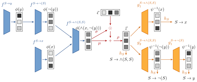
Our proposed architecture is a variational autoencoder for trees, where we construct the encoder as a bottom-up parser, the decoder as a regular tree grammar, and the reconstruction loss as the crossentropy between the true rules generating the input tree and the rules chosen by the decoder. An example autoencoding computation is shown in Figure 2. Because our encoding and decoding schemes are closely related to recursive neural networks (Pollack, 1990; Sperduti and Starita, 1997; Sperduti, 1994), we call our approach recursive tree grammar autoencoders (RTG-AEs). We now introduce each of the components in turn.

3.1 Encoder

Our encoder is a bottom-up parser for a given regular tree grammar $\mathcal{G}=(\Phi,\Sigma,R,S)$, computing a vectorial representation in parallel to parsing. In more detail, we introduce an encoding function $f^{r}:\mathbb{R}^{k\times n}\to\mathbb{R}^{n}$ for each grammar rule $r=(A\to x(B_{1},\ldots,B_{k}))\in R$, which maps the encodings of all children to an encoding of the parent node. Here, $n$ is the encoding dimensionality. As such, the grammar guides our encoding and fixes the number and order of inputs for our encoding functions $f^{r}$. Note that, if $k=0$, $f^{r}$ is a constant.

Next, we apply the functions $f^{r}$ recursively during parsing, yielding a vectorial encoding of the overall tree. More precisely, our encoder $\phi$ is defined by the recursive equation

$$\phi\Big{(}x(\hat{y}_{1},\ldots,\hat{y}_{K}),A\Big{)}=f^{r}(\phi(\hat{y}_{1},B_{1}),\ldots,\phi(\hat{y}_{1},B_{k})),$$ (3)

where $r=A\to x(B_{1},\ldots,B_{k})$ is the first rule in the sequence that generates $x(\hat{y}_{1},\ldots,\hat{y}_{K})$ from $A$. As initial nonterminal $A$, we use the grammar’s starting symbol $S$. Refer to Algorithm 3 for details.

We implement $f^{r}$ as a single-layer feedforward neural network of the form $f^{r}(\vec{y}_{1},\ldots,\vec{y}_{k})=\tanh(\sum_{j=1}^{k}\bm{U}^{r,j}\cdot\vec{y}_{j}+\vec{a}^{r})$, where the weight matrices $\bm{U}^{r,j}\in\mathbb{R}^{n\times n}$ and the bias vectors $\vec{a}^{r}\in\mathbb{R}^{n}$ are parameters to be learned. For optional and starred nonterminals, we further define $f^{B?\to\varepsilon}=f^{B^{*}\to\varepsilon}=\vec{0}$, $f^{B?\to B}(\vec{y})=\vec{y}$, and $f^{B^{*}\to B,B^{*}}(\vec{y}_{1},\vec{y}_{2})=\vec{y}_{1}+\vec{y}_{2}$. In other words, the empty string $\varepsilon$ is encoded as the zero vector, an optional nonterminal is encoded via the identity, and starred nonterminals are encoded via a sum, following the recommendation of Xu et al. (2019) for graph neural nets.

Algorithm 3 Our encoding scheme, as first proposed in (Paaßen et al., 2020), which extends bottom-up parsing for a deterministic regular tree grammar $\mathcal{G}=(\Phi,\Sigma,R,S)$. For each rule $r\in R$ we assume an encoding function $f^{r}$. The algorithm receives a tree as input and returns a nonterminal symbol, a rule sequence that generates the tree from that nonterminal symbol, and a vectorial encoding.

1:function encode(a tree $\hat{x}=x(\hat{y}_{1},\ldots,\hat{y}_{k})$)

2:     for $j\in\{1,\ldots,k\}$ do

3:         $B_{j},\bar{r}_{j},\vec{y}_{j}\leftarrow$ encode($\hat{y}_{j}$).

4:     end for

5:     if $\exists A\in\Phi:A\to x(B_{1},\ldots,B_{k})\in R$ then

6:         $r\leftarrow\big{(}A\to x(B_{1},\ldots,B_{k})\big{)}$.

7:         return $A,(r,\bar{r}_{1},\ldots,\bar{r}_{k}),f^{r}(\vec{y}_{1},\ldots,\vec{y}_{k})$.

8:     else

9:         Error; $\hat{x}$ is not in $\mathcal{L}(\mathcal{G})$.

10:     end if

11:end function

We can show that Algorithm 3 returns without error if and only if the input tree is part of the grammar’s tree language.

Theorem 3.

Let $\mathcal{G}=(\Phi,\Sigma,R,S)$ be a deterministic regular tree grammar. Then, it holds: $\hat{x}$ is a tree in $\mathcal{L}(\mathcal{G})$ if and only if Algorithm 3 returns the nonterminal $S$ as first output. Further, if Algorithm 3 returns with $S$ as first output and some rule sequence $\bar{r}$ as second output, then $\bar{r}$ uniquely generates $\hat{x}$ from $S$. Finally, Algorithm 3 has $\mathcal{O}(\lvert\hat{x}\rvert)$ time and space complexity.

Proof.

Refer to Appendix A.3. ∎

3.2 Decoder

Our decoder is a stochastic version of a given regular tree grammar $\mathcal{G}=(\Phi,\Sigma,R,S)$, controlled by two kinds of neural network. First, for any nonterminal $A\in\Phi$, let $L_{A}$ be the number of rules in $R$ with $A$ on the left hand side. For each $A\in\Phi$, we introduce a linear layer $h_{A}:\mathbb{R}^{n}\to\mathbb{R}^{L_{A}}$ with $h_{A}(\vec{x})=\bm{V}^{A}\cdot\vec{x}+\vec{b}^{A}$. To decode a tree from a vector $\vec{x}\in\mathbb{R}^{n}$ and a nonterminal $A\in\Phi$, we first compute rule scores $\vec{\lambda}=h_{A}(\vec{x})$ and then sample a rule $r_{l}=(A\to x(B_{1},\ldots,B_{k}))\in R$ from the softmax distribution $p_{A}(r_{l}|\vec{x})=\exp(\lambda_{l})/\sum_{l^{\prime}=1}^{L_{A}}\exp(\lambda_{l^{\prime}})$. Then, we apply the sampled rule and use a second kind of neural network to decide the vectorial encodings for each generated child nonterminal $B_{1},\ldots,B_{k}$. In particular, for each grammar rule $r=(A\to x(B_{1},\ldots,B_{k}))\in R$, we introduce $k$ decoding functions $g^{r}_{1},\ldots,g^{r}_{k}:\mathbb{R}^{n}\to\mathbb{R}^{n}$ and compute the vector encoding for the $j$th child as $\vec{y}_{j}=g^{r}_{j}(\vec{x})$. Finally, we decode the children recursively until no nonterminal is left. More precisely, the tree decoding is guided by the recursive equation

$$\psi(\vec{x},A)=x\Big{(}\psi(\vec{y}_{1},B_{1}),\ldots,\psi(\vec{y}_{k},B_{k})\Big{)},$$ (4)

where the rule $r=x\to A(B_{1},\ldots,B_{k})$ is sampled from $p_{A}$ as specified above and $\vec{y}_{j}=g^{r}_{j}(\vec{x})$. As initial nonterminal argument we use the grammar’s starting symbol $S$. For details, refer to Algorithm 4. Note that the time and space complexity is $\mathcal{O}(\lvert\hat{x}\rvert)$ for output tree $\hat{x}$ because each recursion step adds exactly one terminal symbol. Since the entire tree needs to be stored, the space complexity is also $\mathcal{O}(\lvert\hat{x}\rvert)$. Also note that Algorithm 4 is not generally guaranteed to halt (Chi, 1999). In practice, we solve this problem by imposing a maximum number of generated rules.

Algorithm 4 Our decoding scheme, similar to the scheme in (Paaßen et al., 2020), which samples a rule sequence from a regular tree grammar $\mathcal{G}=(\Phi,\Sigma,R,S)$. The algorithm receives a vector $\vec{x}$ and the starting nonterminal $S$ as input and then samples rules with probabilities determined by functions $h_{A}$ for each nonterminal $A\in\Phi$ and decoding functions $g^{r}_{j}$ for each rule $r=A\to x(B_{1},\ldots B_{k})\in R$.

1:function decode(vector $\vec{x}\in\mathbb{R}^{n}$, nonterminal $A\in\Phi$)

2:     Let $r_{1},\ldots,r_{L_{A}}\in R$ be all rules with $A$ on the left hand side.

3:     Compute softmax weights $\vec{\lambda}\leftarrow h_{A}(\vec{x})$.

4:     Sample $r_{l}$ with probability

5:     $\quad p_{A}(r_{l}|\vec{x})=\exp(\lambda_{l})/\sum_{l^{\prime}=1}^{L_{A}}\exp(\lambda_{l^{\prime}})$.

6:     Let $r_{l}=A\to x(B_{1},\ldots,B_{k})$.

7:     for $j\in\{1,\ldots,k\}$ do

8:         $\vec{y}_{j}\leftarrow g^{r_{l}}_{j}(\vec{x})$.

9:         $\hat{y}_{j}\leftarrow$ decode($\vec{y}_{j}$, $B_{j}$).

10:         $\vec{x}\leftarrow\vec{x}-\vec{y}_{j}$.

11:     end for

12:     return $x(\hat{y}_{1},\ldots,\hat{y}_{k})$.

13:end function

An interesting special case are trees that implement lists. For example, consider a carbon chain CCC from chemistry. In the SMILES grammar (Weininger, 1988), this is represented as a binary tree of the form single_chain(single_chain(single_chain(chain_end, C), C), C), i.e. the symbol ‘single_chain’ acts as a list operator. In such a case, we recommend to use a recurrent neural network to implement the decoding function $g^{\text{Chain}\to\text{single\_chain}(\text{Chain},\text{Atom})}_{1}$, such as a gated recurrent unit (GRU) (Cho et al., 2014). In all other cases, we stick with a simple feedforward layer.

3.3 Training

Algorithm 5 A scheme to compute the variational autoencoder (VAE) loss from Equation 2 for our approach. The algorithm receives a tree $\hat{x}$ as input and returns the VAE loss, according to a mean function $\mu$, a standard deviation function $\sigma$, a VAE decoding layer $\rho$, decoding functions $g^{r}_{j}:\mathbb{R}^{n}\to\mathbb{R}^{n}$, and VAE hyperparameters $s,\beta\in\mathbb{R}^{+}$.

1:function loss(a tree $\hat{x}$)

2:     $A,(r_{1},\ldots,r_{T}),\vec{x}\leftarrow$ encode($\hat{x}$) via Algorithm 3.

3:     $\vec{\mu}\leftarrow\mu(\vec{x})$. $\quad\vec{\sigma}\leftarrow\sigma(\vec{x})$. $\quad\vec{\epsilon}\sim\mathcal{N}(\vec{0}|s\cdot\bm{I}^{n_{\mathrm{VAE}}})$.

4:     $\vec{z}\leftarrow\rho(\vec{\mu}+\vec{\epsilon}\odot\vec{\sigma})$.

5:     Initialize a stack $\mathcal{S}$ with $\vec{z}$ on top.

6:     Initialize $\ell\leftarrow\beta\cdot\big{(}\sum_{j=1}^{n_{\mathrm{VAE}}}\mu_{j}^{2}+\sigma_{j}^{2}-\log[\sigma_{j}^{2}]-1\big{)}$.

7:     for $t\leftarrow 1,\ldots,T$ do

8:         Let $r_{t}=A\to x(B_{1},\ldots,B_{k})$.

9:         Pop $\vec{x}_{t}$ from the top of $\mathcal{S}$.

10:         Compute $p_{A}(r_{t}|\vec{x}_{t})$ as in line 5 of Algorithm 4.

11:         $\ell\leftarrow\ell-\log\big{[}p_{A}(r_{t}|\vec{x}_{t})\big{]}$.

12:         for $j\leftarrow 1,\ldots,k$ do

13:              $\vec{y}_{j}\leftarrow g^{r_{t}}_{j}(\vec{x}_{t})$.

14:              $\vec{x}_{t}\leftarrow\vec{x}_{t}-\vec{y}_{j}$.

15:         end for

16:         Push $\vec{y}_{k},\ldots,\vec{y}_{1}$ onto $\mathcal{S}$.

17:     end for

18:     return $\ell$.

19:end function

We train our recursive tree grammar autoencoder (RTG-AE) in the variational autoencoder (VAE) framework, i.e. we try to minimize the loss in Equation 2. More precisely, we define the encoding probability density $q_{\phi}(\vec{z}|\hat{x})$ as the Gaussian with mean $\mu(\phi(\hat{x}))$ and covariance matrix $\mathrm{diag}\big{[}\sigma(\phi(\hat{x}))\big{]}$, where the functions $\mu:\mathbb{R}^{n}\to\mathbb{R}^{n_{\mathrm{VAE}}}$ and $\sigma:\mathbb{R}^{n}\to\mathbb{R}^{n_{\mathrm{VAE}}}$ are defined as

$$\mu(\vec{x}) =\bm{U}^{\mu}\cdot\vec{x}+\vec{a}^{\mu},$$

$$\sigma(\vec{x}) =\exp\big{(}\frac{1}{2}\cdot[\bm{U}^{\sigma}\cdot\vec{x}+\vec{a}^{\sigma}]\big{)},$$ (5)

where $\bm{U}^{\mu},\bm{U}^{\sigma}\in\mathbb{R}^{n_{\mathrm{VAE}}\times n}$ and $\vec{a}^{\mu},\vec{a}^{\sigma}\in\mathbb{R}^{n_{\mathrm{VAE}}}$ are additional parameters.

To decode, we first transform the encoding vector $\vec{z}$ with a single layer $\rho(\vec{z})=\tanh\big{(}\bm{W}^{\rho}\cdot\vec{z}+\vec{c}^{\rho}\big{)}$ and then apply the decoding scheme from Algorithm 4. As the decoding probability $p_{\psi}(\hat{x}|\vec{z})$, we use the product over all probabilities $p_{A}(r_{t}|\vec{x}_{t})$ from line 5 of Algorithm 4, i.e. the probability of always choosing the correct grammar rule during decoding, provided that all previous choices have already been correct. The negative logarithm of this product can also be interpreted as the crossentropy loss between the correct rule sequence and the softmax probabilities from line 5 of Algorithm 4. The details of our loss computation are given in Algorithm 5. Note that the time and space complexity is $\mathcal{O}(\lvert\hat{x}\rvert)$ because the outer loop from line 7-17 runs $T=\lvert\hat{x}\rvert$ times, and the inner loop in lines 12-15 runs $\lvert\hat{x}\rvert-1$ times in total because every node takes the role of child exactly once (except for the root). Because the loss is differentiable, we can optimize it using gradient descent schemes such as Adam (Kingma and Ba, 2015). The gradient computation is performed by the pyTorch autograd system (Paszke et al., 2019).

4 Experiments and Discussion

	Boolean	Expressions	SMILES	Pysort
dataset size	$34,884$	$104,832$	$249,456$	$294$
avg. tree size	$5.21$	$8.95$	$83.66$	$57.97$
avg. depth	$3.18$	$4.32$	$21.29$	$9.25$
max. rule seq. length	$14$	$11$	$285$	$168$
no. symbols	$5$	$9$	$43$	$54$
no. grammar rules	$5$	$9$	$46$	$54$

Table 1: The statistics for all four dataset.

model	Boolean	Expressions	SMILES	Pysort
D-VAE	$249,624$	$252,828$	$1,979,038$	$1,859,417$
GVAE	$198,316$	$197,536$	$1,928,431$	$1,630,263$
TES-AE	$500$	$900$	$11,776$	$13,824$
GRU-TG-AE	$67,221$	$70,025$	$437,080$	$445,280$
RTG-AE	$104,021$	$165,125$	$5,161,816$	$5,493,600$

Table 2: The number of parameters for all models on all datasets.

We evaluate the performance of RTG-AEs on four datasets (refer to Table 1 for statistics), namely:

Boolean: Randomly sampled Boolean formulae over the variables $x$ and $y$ with at most three binary operators, e.g. $x\wedge\neg y$ or $x\wedge y\wedge(x\vee\neg y)$.

Expressions: Randomly sampled algebraic expressions over the variable $x$ of the form $3*x+\sin(x)+\exp(2/x)$, i.e. consisting of a binary operator plus a unary operator plus a unary of a binary. This dataset is taken from (Kusner et al., 2017).

SMILES: Roughly 250k chemical molecules as SMILES strings (Weininger, 1988), as selected by (Kusner et al., 2017).

Pysort: 29 Python sorting programs and manually generated preliminary development stages of these programs, resulting in 294 programs overall.

model	Boolean	Expressions	SMILES	Pysort
D-VAE	$4.32\pm 0.41$	$5.84\pm 0.32$	$132.70\pm 57.02$	$70.67\pm 7.20$
GVAE	$3.61\pm 0.51$	$5.84\pm 2.00$	$594.92\pm 5.99$	$61.44\pm 5.18$
TES-AE	$2.62\pm 0.26$	$2.09\pm 0.18$	$581.08\pm 25.99$	$\bm{20.40\pm 4.27}$
GRU-TG-AE	$1.98\pm 0.53$	$3.70\pm 0.31$	$482.88\pm 129.52$	$93.63\pm 1.44$
RTG-AE	$\bm{0.83\pm 0.23}$	$\bm{0.77\pm 0.23}$	$\bm{111.14\pm 159.97}$	$38.14\pm 3.63$

Table 3: The average autoencoding RMSE ($\pm$ standard deviation).

model	Boolean	Expressions	SMILES	Pysort
D-VAE	$882.0\pm 45.9$	$1201.5\pm 24.8$	$64225.9\pm 4,500.3$	$66789.9\pm 3555.2$
GVAE	$1316.5\pm 86.7$	$1218.8\pm 73.8$	$7771.2\pm 1,524.2$	$1393.7\pm 120.9$
TES-AE	$\bm{0.9\pm 0.1}$	$\bm{1.5\pm 0.2}$	$\bm{583.6\pm 103.6}$	$\bm{10.1\pm 0.6}$
GRU-TG-AE	$440.8\pm 30.4$	$734.5\pm 50.8$	$3342.2\pm 42.7$	$648.6\pm 50.1$
RTG-AE	$221.5\pm 4.7$	$357.4\pm 13.2$	$1903.4\pm 34.1$	$399.9\pm 21.9$

Table 4: The average runtime in seconds ($\pm$ standard deviation) as measured by Python.

We compare RTG-AEs to three baseline models from the literature, namely grammar variational autoencoders (GVAE) (Kusner et al., 2017), directed acyclic graph variational autoencoders (D-VAE) (Zhang et al., 2019b), and tree echo state autoencoders (TES-AE) (Paaßen et al., 2020). Additionally, we compare to a recurrent version of tree grammar AEs (GRU-TG-AEs), i.e. we represent a tree by its rule sequence and autoencode it with a gated recurrent unit (GRU) (Cho et al., 2014). We also performed preliminary experiments with semantic constraints akin to (Dai et al., 2018) but did not obtain significantly different results, such that we omit such constraints here for simplicity. Note that our baselines are selected to implement an ablation study: GVAE and GRU-TG-AE use grammar knowledge and variational autoencoding (VAE), but not recursive processing; TES-AE uses grammar knowledge and recursive processing, but not VAE; and D-VAE uses graph-like processing and VAE but no grammar knowledge.

We used the reference implementation and architecture of all approaches, with a slight difference for GVAE, where we ported the reference implementation from Keras to pyTorch in order to be comparable to all other approaches. The number of parameters for all models on all datasets is shown in Table 2. We trained all neural networks using Adam (Kingma and Ba, 2015) with a learning rate of $10^{-3}$ and a ReduceLROnPlateau scheduler with minimum learning rate $10^{-4}$, following the learning procedure of Kusner et al. (2017) as well as Dai et al. (2018). We sampled 100k trees for the first two and 10k trees for the latter two datasets. To obtain statistics, we repeated the training ten times with different samples (by generating new data for boolean and expressions and by doing a 10-fold crossvalidation for SMILES and pysort). Following Zhang et al. (2019b), we used a batch size of $32$ for all approaches. For each approach and each dataset, we optimized the hyper-parameters $\beta$ and $s$ of Equations 2 and 5 in a random search with 20 trials over the range $[10^{-5},1]$, using separate data. For the first two data sets, we set $n=100$ and $n_{\mathrm{VAE}}=8$, whereas for the latter two we set $n=256$ and $n_{\mathrm{VAE}}=16$. For TES-AE, we followed the protocol of Paaßen et al. (2020), training on a random subset of $500$ training data points, and we optimized the sparsity, spectral radius, regularization strength with the same hyper-parameter optimization scheme.

Figure 3: A 2D t-SNE reduction of the codes of 1000 random molecules from the SMILES data set by GVAE (left), TES-AE (center), and RTG-AE (right). Color indicates the objective function value. Rectangles indicate the $30$-means cluster with highest mean objective function value $\pm$ std.

model	Boolean	Expressions	SMILES	Pysort
D-VAE	$28.8\%$	$23.8\%$	$0.1\%$	$1.4\%$
GVAE	$90.4\%$	$99.8\%$	$0\%$	$99.9\%$
GRU-TG-AE	$99.9\%$	$98.2\%$	$5.9\%$	$0\%$
RTG-AE	$98.5\%$	$99.6\%$	$37.3\%$	$99.7\%$

Table 5: The rate of syntactically correct trees decoded from standard normal random vectors.

model	median tree	median score
	Expressions
D-VAE	x	$0.49\pm 0.00$
GVAE	x + 1 + sin(3 + 3)	$0.46\pm 0.00$
TES-AE	x	$0.49\pm 0.00$
GRU-TG-AE	x	$0.49\pm 0.00$
RTG-AE	x + 1 + sin(x * x)	$\bm{0.33\pm 0.05}$
	SMILES
GVAE	n.a.	n.a.
TES-AE	CCO	$-0.31\pm 0.50$
GRU-TG-AE	C=C	$-2.23\pm 1.56$
RTG-AE	CCCCCCC	$\bm{2.57\pm 0.31}$

Table 6: The optimization scores for the Expressions (lower is better) and SMILES (higher is better) with median tree and median score ($\pm\frac{1}{2}$ IQR).

The SMILES experiment was performed on a computation server with a 24core CPU and 48GB RAM, whereas all other experiments were performed on a consumer grade laptop with Intel i7 4core CPU and 16GB RAM. All experimental code, including all grammars and implementations, is available at https://gitlab.com/bpaassen/rtgae.

We measure autoencoding error on test data in terms of the root mean square tree edit distance (Zhang and Shasha, 1989). We use the root mean square error (RMSE) rather than log likelihood because D-VAE measures log likelihood different to GVAE, GRU-TG-AE, and RTG-AE, and TES-AE does not measure log likelihood at all. By contrast, the RMSE is agnostic to the underlying distribution model. Further, we use the tree edit distance as a tree metric because it is defined on all possible labeled trees without regard for the underlying distribution or grammar and hence does not favor any of the models (Bille, 2005).

The RMSE results are shown in Table 3. We observe that RTG-AEs achieve notably lower errors compared to all baselines on all datasets ($p<0.05$ in a Wilcoxon signed rank test, except for D-VAE on SMILES, where $p>0.05$, and TES-AE on pysort, where RTG-AEs were worse). We also note that, among all deep learning approaches, RTG-AEs have the lowest training times, speeding up at least one third over the fastest other baseline, GRU-TG-AEs (refer to Table 4). Only TES-AEs are notably faster because they do not require backpropagation. We explain these results by the fact that all three defining features of RTG-AEs contribute to a low error: Compared to D-VAEs, RTG-AEs exploit the inductive bias provided by a regular tree grammar and can, hence, achieve a lower error with less training. Compared to GVAEs and GRU-TG-AEs, RTG-AEs use recursive processing, which means that information only needs to be remembered across the depth of a tree, not across the number of nodes. This means that a smaller model suffices to achieve the desired memory capacity. Finally, compared to TES-AEs, RTG-AEs train the autoencoder end-to-end in a variational autoencoder framework which gives the model much more ability to adjust to the data set at hand. However, we notice that these additional degrees of freedom only help if the data set is large enough: For pysort, by far the smallest data set, TES-AEs do better.

To evaluate the ability of all models to generate syntactically valid trees, we sampled 1000 standard normal random vectors and decoded them with all models. Then, we checked their syntax with a bottom-up regular tree parser for the language. The percentage of correct trees is shown in Table 5. Unsurprisingly, D-VAE has the worst results across the board because it does not use grammatical knowledge for decoding. In principle, the other models should always have 100% because their architecture guarantees syntactic correctness. Instead, we observe that the rates drop far below 100% for GRU-TG-AE on Pysort and for all models on SMILES. This is because the decoding process can fail if it gets stuck in a loop. Even on the SMILES dataset, though, the RTG-AE achieves the best rate.

We also repeated the optimization experiments of Kusner et al. (2017) in the latent space of the Expressions and SMILES datasets. We used the same objective functions as Kusner et al. (2017); i.e. the log MSE to the ground truth expression $\frac{1}{3}+x+\sin(x*x)$ for Expressions and a mixture of logP, synthetic availability, and cycle length for SMILES. For SMILES, we further retrained all models (except D-VAE due to memory constraints) with $n_{\mathrm{VAE}}=56$ and 50k training samples to have the same model capacity and training set size as Kusner et al. (2017). In contrast to Kusner et al. (2017), we used CMA-ES instead of Bayesian optimization because we could not get the original Bayesian Optimization implementation to run within reasonable effort, whereas the Python cma package worked out-of-the-box. CMA-ES is a usual method for high-dimensional, gradient-free optimization that has shown competitive results to Bayesian optimization for neural network optimization (Loshchilov and Hutter, 2016). It also is particularly well suited to the latent space of VAEs because CMA-ES samples its population from a Gaussian distribution. We used $15$ iterations and a computational budget of $750$ trees, as Kusner et al. (2017). To obtain statistics, we performed the optimization 10 times for each approach.

The median results ($\pm$ inter-quartile ranges) are shown in Table 6. We observe that RTG-AEs significantly outperform all baselines on both data sets ($p<0.01$ in a Wilcoxon rank-sum test) by a difference of several inter-quartile ranges. For SMILES, CMA-ES couldn’t find any semantically valid molecule for GVAE and achieved a negative median score for all methods but RTG-AE. We note that, on both data sets, Bayesian optimization performed better than CMA-ES (Kusner et al., 2017). Still, our results show that even the weaker CMA-ES optimizer can consistently achieve good scores in the RTG-AE latent space. We believe there are two reasons for this: First, the higher rate of syntactically correct trees for RTG-AE (refer to Table 5); second, because recursive processing tends to cluster similar trees together (Paaßen et al., 2020; Tiňo and Hammer, 2003) in a fractal fashion, such that an optimizer only needs to find a viable cluster and optimize within it. Figure 3 shows a t-SNE visualization of the latent spaces, revealing that the recursive models provide more distinct clusters, compared to GVAE, and that trees inside the cluster with best objective function value have lower variance compared to GVAE.

5 Conclusion

In this contribution, we introduced the recursive tree grammar autoencoder (RTG-AE), a novel neural network architecture that combines variational autoencoders with recursive neural networks and regular tree grammars. In particular, our approach encodes a tree with a bottom-up parser, and decodes it with a tree grammar, both learned via neural networks and variational autoencoding. In an ablation study, we showed that the unique combination of recursive processing, grammatical knowledge, and variational autoencoding improves autoencoding error, training time, and optimization performance beyond existing models that use only two of these concepts, but not all three. This finding can be explained by three conceptual observations: First, recursive processing follows the tree structure whereas sequential processing introduces long-range dependencies between children and parents in the tree; second, grammatical knowledge avoids obvious decoding mistakes by limiting the terminal symbols we can choose; third, variational autoencoding encourages a smooth encoding space, whereas a random encoding may exhibit unfavourable structure for sampling and optimization. Theoretically, we proved that RTG-AEs parse and generate trees in linear time and are expressive enough for all regular tree languages.

In future work, one could replace more encoders and decoders with recurrent networks, such as Tree-LSTMs, and one could impose more domain-specific semantic constraints as well as post-processing mechanisms to tailor RTG-AEs to specific application domains.

Appendix A Proofs

For the purpose of our tree language proofs, we first introduce a few auxiliary concepts. First, we extend the definition of a regular tree grammar slightly to permit multiple starting symbols. In particular, we re-define a regular tree grammar as a $4$-tuple $\mathcal{G}=(\Phi,\Sigma,R,\mathcal{S})$, where $\Phi$ and $\Sigma$ are disjoint finite sets and $R$ is a rule set as before, but $\mathcal{S}$ is now a subset of $\Phi$. Next, we define the partial tree language $\mathcal{L}(\mathcal{G}|A)$ for nonterminal $A\in\Phi$ as the set of all trees which can be generated from nonterminal $A$ using rule sequences from $R$. Further, we define the $n$-restricted partial language $\mathcal{L}_{n}(\mathcal{G}|A)$ for nonterminal $A\in\Phi$ as the set $\mathcal{L}_{n}(\mathcal{G}|A):=\big{\{}\hat{x}\in\mathcal{L}(\mathcal{G}|A)\big{|}|\hat{x}|\leq n\big{\}}$, i.e. it includes only the trees up to size $n$. We define the tree language $\mathcal{L}(\mathcal{G})$ of $\mathcal{G}$ as the union $\mathcal{L}(\mathcal{G}):=\bigcup_{S\in\mathcal{S}}\mathcal{L}(\mathcal{G}|S)$.

As a final preparation, we introduce a straightforward lemma regarding restricted partial tree languages.

Lemma 1.

Let $\mathcal{G}=(\Phi,\Sigma,R,\mathcal{S})$ be a regular tree grammar.

Then, for all $A\in\Phi$, all $n\in\mathbb{N}$ and all trees $\hat{x}$ it holds: $\hat{x}=x(\hat{y}_{1},\ldots,\hat{y}_{k})$ is in $\mathcal{L}_{n}(\mathcal{G}|A)$ if and only if there exist nonterminals $B_{1},\ldots,B_{k}\in\Phi$ such that $A\to x(B_{1},\ldots,B_{k})\in R$ and $\hat{y}_{j}\in\mathcal{L}_{n_{j}}(\mathcal{G}|B_{j})$ for all $j\in\{1,\ldots,k\}$ with $n_{1}+\ldots+n_{k}=n-1$.

Proof.

If $\hat{x}\in\mathcal{L}_{n}(\mathcal{G}|A)$, then there exists a sequence of rules $r_{1},\ldots,r_{T}\in R$ which generates $\hat{x}$ from $A$. The first rule in that sequence must be of the form $A\to x(B_{1},\ldots,B_{k})$, otherwise $\hat{x}$ would not have the shape $\hat{x}=x(\hat{y}_{1},\ldots,\hat{y}_{k})$. Further, $r_{2},\ldots,r_{T}$ must consist of subsequences $\bar{r}_{1},\ldots,\bar{r}_{k}=r_{2},\ldots,r_{T}$ such that $\bar{r}_{j}$ generates $\hat{y}_{j}$ from $B_{j}$ for all $j\in\{1,\ldots,k\}$, otherwise $\hat{x}\neq x(\hat{y}_{1},\ldots,\hat{y}_{k})$. However, that implies that $\hat{y}_{j}\in\mathcal{L}(\mathcal{G}|B_{j})$ for all $j\in\{1,\ldots,k\}$. The length restriction to $n_{j}$ follows because—per definition of the tree size—the sizes $|\hat{y}_{j}|$ must add up to $|\hat{x}|-1$.

Conversely, if there exist nonterminals $B_{1},\ldots,B_{k}\in\Phi$ such that $r=A\to x(B_{1},\ldots,B_{k})\in R$ and $\hat{y}_{j}\in\mathcal{L}_{n_{j}}(\mathcal{G}|B_{j})$ for all $j\in\{1,\ldots,k\}$, then there must exist rule sequences $\bar{r}_{1},\ldots,\bar{r}_{k}$ which generate $\hat{y}_{j}$ from $B_{j}$ for all $j\in\{1,\ldots,k\}$. Accordingly, $r,\bar{r}_{1},\ldots,\bar{r}_{k}$ generates $\hat{x}$ from $A$ and, hence, $\hat{x}\in\mathcal{L}(\mathcal{G}|A)$. The length restriction follows because $|\hat{x}|=1+|\hat{y}_{1}|+\ldots+|\hat{y}_{k}|\leq 1+n_{1}+\ldots+n_{k}=n$. ∎

A.1 Deterministic grammars imply unique rule sequences

Recall that we define a regular tree grammar as deterministic if no two rules have the same right-hand-side. Our goal is to show that every deterministic regular tree grammar is unambiguous, in the sense that there always exists a unique rule sequence generating the tree. We first prove an auxiliary result.

Lemma 2.

Let $\mathcal{G}=(\Phi,\Sigma,R,S)$ be a deterministic regular tree grammar. Then, for any two $A\neq A^{\prime}\in\Phi$, $\mathcal{L}(\mathcal{G}|A)\cap\mathcal{L}(\mathcal{G}|A^{\prime})=\emptyset$.

Proof.

We perform a proof via induction over the tree size. First, consider trees $\hat{x}$ with $\lvert\hat{x}\rvert=1$, that is, $\hat{x}=x()$. If $\hat{x}\in\mathcal{L}(\mathcal{G}|A)$ for some $A\in\Phi$, the rule $A\to x()$ must be in $R$. Because $\mathcal{G}$ is deterministic, there can exist no $A^{\prime}\neq A\in\Phi$ with $A^{\prime}\to x()\in R$, otherwise there would be two rules with the same right-hand-side. Accordingly, $\hat{x}$ lies in $\mathcal{L}(\mathcal{G}|A)$ for at most one $A\in\Phi$.

Now, assume that the claim holds for all trees up to size $n$ and consider a tree $\hat{x}$ with $\lvert\hat{x}\rvert=n+1$. Without loss of generality, let $\hat{x}=x(\hat{y}_{1},\ldots,\hat{y}_{k})$. If $\hat{x}\in\mathcal{L}(\mathcal{G}|A)$ for some $A\in\Phi$, a rule of the form $A\to x(B_{1},\ldots,B_{k})$ must be in $R$, such that for all $j\in\{1,\ldots,k\}$: $\hat{y}_{j}\in\mathcal{L}(\mathcal{G}|B_{j})$. Now, note that $\lvert\hat{y}_{j}\rvert\leq n$. Accordingly, our induction hypothesis applies and there exists no other $B^{\prime}_{j}\neq B_{j}$ such that $\hat{y}_{j}\in\mathcal{L}(\mathcal{G}|B^{\prime}_{j})$. Further, there can exist no $A^{\prime}\neq A$ with $A^{\prime}\to x(B_{1},\ldots,B_{k})$, otherwise there would be two rules with the same right-hand-side. Accordingly, $\hat{x}$ lies in $\mathcal{L}(\mathcal{G}|A)$ for at most one $A\in\Phi$. ∎

Now, we prove the desired result.

Theorem 4.

Let $\mathcal{G}=(\Phi,\Sigma,R,S)$ be a deterministic regular tree grammar. Then, for any $\hat{x}\in\mathcal{L}(\mathcal{G})$ there exists exactly one sequence of rules $r_{1},\ldots,r_{T}\in R$ which generates $\hat{x}$ from $S$.

Proof.

In fact, we will prove a more general result, namely that the claim holds for all $\hat{x}\in\bigcup_{A\in\Phi}\mathcal{L}(\mathcal{G}|A)$. We perform an induction over the tree size.

First, consider trees $\hat{x}$ with $\lvert\hat{x}\rvert=1$, that is, $\hat{x}=x()$. Then, the only way to generate $\hat{x}$ is by applying a single rule of the form $A\to x()$. Because $\mathcal{G}$ is deterministic, only one such rule can exist. Therefore, the claim holds.

Now, assume that the claim holds for all trees up to size $n$ and consider a tree $\hat{x}$ with $\lvert\hat{x}\rvert=n+1$. Without loss of generality, let $\hat{x}=x(\hat{y}_{1},\ldots,\hat{y}_{k})$. If $\hat{x}\in\mathcal{L}(\mathcal{G}|A)$ for some $A\in\Phi$, then there must exist a rule of the form $A\to x(B_{1},\ldots,B_{k})$ in $R$, such that for all $j\in\{1,\ldots,k\}$: $\hat{y}_{j}\in\mathcal{L}(\mathcal{G}|B_{j})$. Due to the previous lemma and our induction hypothesis we know that for each $j$, there exists a unique nonterminal $B_{j}$ and rule sequence $\bar{r}_{j}$, such that $\bar{r}_{j}$ generates $\hat{y}_{j}$ from $B_{j}$. Further, because $\mathcal{G}$ is deterministic, there can exist no other $A^{\prime}\neq A\in\Phi$, such that $A^{\prime}\to x(B_{1},\ldots,B_{k})$ in $R$. Therefore, the rule $A\to x(B_{1},\ldots,B_{k})$ concatenated with the rule sequences $\bar{r}_{1}$, $\ldots$, $\bar{r}_{k}$ is the only way to generate $\hat{x}$, as claimed. ∎

A.2 All regular tree grammars can be made deterministic

Theorem 5.

Let $\mathcal{G}=(\Phi,\Sigma,R,\mathcal{S})$ be a regular tree grammar. Then, there exists a regular tree grammar $\mathcal{G}^{\prime}=(\Phi^{\prime},\Sigma,R^{\prime},\mathcal{S}^{\prime})$ which is deterministic and where $\mathcal{L}(\mathcal{G})=\mathcal{L}(\mathcal{G}^{\prime})$.

Proof.

This proof is an adaptation of Theorem 1.1.9 of Comon et al. [2008] and can also be seen as an analogue to conversion from nondeterministic finite state machines to deterministic finite state machines.

In particular, we convert $\mathcal{G}$ to $\mathcal{G}^{\prime}$ via the following procedure.

We first initialize $\Phi^{\prime}$ and $R^{\prime}$ as empty sets.

Second, iterate over $k$, starting at zero up to the maximum number of children in a rule in $R$, and iterate over all right-hand-sides $x(B_{1},\ldots,B_{k})$ that occur in rules in $R$. Next, we collect all $A_{1},\ldots,A_{m}\in\Phi$ such that $A_{i}\to x(B_{1},\ldots,B_{k})\in R$ and add the set $A^{\prime}=\{A_{1},\ldots,A_{m}\}$ to $\Phi^{\prime}$.

Third, we perform the same iteration again, but this time we add grammar rules $\{A_{1},\ldots,A_{m}\}\to x(B_{1}^{\prime},\ldots,B_{k}^{\prime})$ to $R^{\prime}$ for all combinations $B^{\prime}_{1},\ldots,B^{\prime}_{k}\in\Phi^{\prime}$ where $B_{j}\in B^{\prime}_{j}$ for all $j\in\{1,\ldots,k\}$.

Finally, we define $\mathcal{S}^{\prime}=\{A^{\prime}\in\Phi^{\prime}|A^{\prime}\cap\mathcal{S}\neq\emptyset\}$.

It is straightforward to see that $\mathcal{G}^{\prime}$ is deterministic because all rules with the same right-hand-side get replaced with rules with a unique left-hand-side.

It remains to show that the generated tree languages are the same. To that end, we first prove an auxiliary claim, namely that for all $A\in\Phi$ it holds: A tree $\hat{x}$ is in $\mathcal{L}_{n}(\mathcal{G}|A)$ if and only if there exists an $A^{\prime}\in\Phi^{\prime}$ with $A\in A^{\prime}$ and $\hat{x}\in\mathcal{L}_{n}(\mathcal{G}^{\prime}|A^{\prime})$.

We show this claim via induction over $n$. First, consider $n=1$. If $\hat{x}\in\mathcal{L}_{1}(\mathcal{G}|A)$, $\hat{x}$ must have the shape $\hat{x}=x()$, otherwise $|\hat{x}|>1$, and the rule $A\to x()$ must be in $R$. Accordingly, our procedure assures that there exists some $A^{\prime}\in\Phi^{\prime}$ with $A\in A^{\prime}$ and $A^{\prime}\to x()\in R^{\prime}$. Hence, $\hat{x}\in\mathcal{L}_{1}(\mathcal{G}^{\prime}|A^{\prime})$.

Conversely, if $\hat{x}\in\mathcal{L}_{1}(\mathcal{G}^{\prime}|A^{\prime})$ for some $A^{\prime}\in\Phi^{\prime}$ then $\hat{x}$ must have the shape $\hat{x}=x()$, otherwise $|\hat{x}|>1$, and the rule $A^{\prime}\to x()$ must be in $R^{\prime}$. However, this rule can only be in $R^{\prime}$ if for any $A\in A^{\prime}$ the rule $A\to x()$ was in $R$. Accordingly, $\hat{x}\in\mathcal{L}_{1}(\mathcal{G}|A)$.

Now, consider the case $n>1$ and let $\hat{x}=x(\hat{y}_{1},\ldots,\hat{y}_{k})$. If $\hat{x}\in\mathcal{L}_{n}(\mathcal{G}|A)$, Lemma 1 tells us that there must exist nonterminals $B_{1},\ldots,B_{k}\in\Phi$ such that $A\to x(B_{1},\ldots,B_{k})\in R$ and $\hat{y}_{j}\in\mathcal{L}_{n_{j}}(\mathcal{G}|B_{j})$ for all $j\in\{1,\ldots,k\}$ with $n_{1}+\ldots+n_{k}=n-1$. Hence, by induction we know that there exist $B^{\prime}_{j}\in\Phi^{\prime}$ such that $B_{j}\in B^{\prime}_{j}$ and $\hat{y}_{j}\in\mathcal{L}_{n_{j}}(\mathcal{G}^{\prime}|B^{\prime}_{j})$ for all $j\in\{1,\ldots,k\}$. Further, our procedure for generating $\mathcal{G}^{\prime}$ ensures that there exists some $A^{\prime}\in\Phi^{\prime}$ such that the rule $A^{\prime}\to x(B^{\prime}_{1},\ldots,B^{\prime}_{k})$ is in $R^{\prime}$. Hence, Lemma 1 tells us that $\hat{x}\in\mathcal{L}_{n}(\mathcal{G}^{\prime}|A^{\prime})$.

Conversely, if $\hat{x}\in\mathcal{L}_{n}(\mathcal{G}^{\prime}|A^{\prime})$ then Lemma 1 tells us that there must exist nonterminals $B^{\prime}_{1},\ldots,B^{\prime}_{k}\in\Phi^{\prime}$ such that $A^{\prime}\to x(B^{\prime}_{1},\ldots,B^{\prime}_{k})\in R^{\prime}$ and $\hat{y}_{j}\in\mathcal{L}_{n_{j}}(\mathcal{G}^{\prime}|B^{\prime}_{j})$ for all $j\in\{1,\ldots,k\}$ with $n_{1}+\ldots+n_{k}=n-1$. Hence, by induction we know that for all $j\in\{1,\ldots,k\}$ and all $B_{j}\in B^{\prime}_{j}$ we obtain $\hat{y}_{j}\in\mathcal{L}_{n_{j}}(\mathcal{G}|B_{j})$. Further, our procedure for generating $\mathcal{G}^{\prime}$ ensures that for any $A\in A^{\prime}$ there must exist a rule $A\to x(B_{1},\ldots,B_{k})\in R$ for some $B_{1},\ldots,B_{k}\in\Phi$ and $B_{j}\in B^{\prime}_{j}$ for some combination of $B^{\prime}_{j}\in\Phi^{\prime}$. Hence, Lemma 1 tells us that $\hat{x}\in\mathcal{L}_{n}(\mathcal{G}|A)$. This concludes the induction.

Now, note that $\hat{x}\in\mathcal{L}(\mathcal{G})$ implies that there exists some $S\in\mathcal{S}$ with $\hat{x}\in\mathcal{L}(\mathcal{G}|S)$. Our auxiliary result tells us that there then exists some $S^{\prime}\in\Phi^{\prime}$ with $S\in\Phi^{\prime}$ and $\hat{x}\in\mathcal{L}(\mathcal{G}^{\prime}|S^{\prime})$. Further, since $S^{\prime}\cup\mathcal{S}$ contains at least $S$, our construction of $\mathcal{G}^{\prime}$ implies that $S^{\prime}\in\mathcal{S}^{\prime}$. Hence, $\hat{x}\in\mathcal{L}(\mathcal{G}^{\prime})$.

Conversely, if $\hat{x}\in\mathcal{L}(\mathcal{G}^{\prime})$, there must exist some $S^{\prime}\in\mathcal{S}^{\prime}$ with $\hat{x}\in\mathcal{L}(\mathcal{G}^{\prime}|S^{\prime})$. Since $S^{\prime}\in\mathcal{S}^{\prime}$, there must exist at least one $S\in S^{\prime}$ such that $S\in\mathcal{S}$. Further, our auxiliary result tells us that $\hat{x}\in\mathcal{L}(\mathcal{G}|S)$. Accordingly, $\hat{x}\in\mathcal{L}(\mathcal{G})$. ∎

As an example, consider the following grammar $\mathcal{G}=(\Phi,\Sigma,R,\mathcal{S})$ for logical formulae in conjuctive normal form.

$$\Phi=\{ F,C,L,A\}$$

$$\Sigma=\{ \wedge,\vee,\neg,x,y\}$$

$$R=\{ F\to\wedge(C,F)|\vee(L,C)|\neg(A)|x|y,$$

$$C\to\vee(L,C)|\neg(A)|x|y,$$

$$L\to\neg(A)|x|y,$$

$$A\to x|y\}$$

$$\mathcal{S}=\{ F\}$$

The deterministic version of this grammar is $\mathcal{G}^{\prime}=(\Phi^{\prime},\Sigma,R^{\prime},\mathcal{S}^{\prime})$ with $\mathcal{S}^{\prime}=\Phi^{\prime}$ and

$$\Phi^{\prime}=\{ \{F,C,L,A\},\{F,C,L\},\{F,C\},\{F\}\}$$

$$R^{\prime}=\Big{\{} \{F,C,L,A\}\to x|y,$$

$$\{F,C,L\}\to\neg(\{F,C,L,A\}),$$

$$\{F,C\}\to\vee(\{F,C,L,A\},\{F,C,L,A\}),$$

$$\{F,C\}\to\vee(\{F,C,L,A\},\{F,C,L\}),$$

$$\{F,C\}\to\vee(\{F,C,L,A\},\{F,C\}),$$

$$\{F,C\}\to\vee(\{F,C,L\},\{F,C,L,A\}),$$

$$\{F,C\}\to\vee(\{F,C,L\},\{F,C,L\}),$$

$$\{F,C\}\to\vee(\{F,C,L\},\{F,C\}),$$

$$\{F\}\to\wedge(\{F,C,L,A\},\{F,C,L,A\}),$$

$$\{F\}\to\wedge(\{F,C,L,A\},\{F,C,L\}),$$

$$\{F\}\to\wedge(\{F,C,L,A\},\{F,C\}),$$

$$\{F\}\to\wedge(\{F,C,L,A\},\{F\}),$$

$$\{F\}\to\wedge(\{F,C,L\},\{F,C,L,A\}),$$

$$\{F\}\to\wedge(\{F,C,L\},\{F,C,L\}),$$

$$\{F\}\to\wedge(\{F,C,L\},\{F,C\}),$$

$$\{F\}\to\wedge(\{F,C,L\},\{F\}),$$

$$\{F\}\to\wedge(\{F,C\},\{F,C,L,A\}),$$

$$\{F\}\to\wedge(\{F,C\},\{F,C,L\}),$$

$$\{F\}\to\wedge(\{F,C\},\{F,C\}),$$

$$\{F\}\to\wedge(\{F,C\},\{F\})\Big{\}}.$$

A.3 Proof of the Parsing Theorem

We first generalize the statement of the theorem to also work for regular tree grammars with multiple starting symbols. In particular, we show the following:

Theorem 6.

Let $\mathcal{G}=(\Phi,\Sigma,R,\mathcal{S})$ be a deterministic regular tree grammar. Then, it holds: $\hat{x}$ is a tree in $\mathcal{L}(\mathcal{G})$ if and only if Algorithm 3 returns a nonterminal $S\in\mathcal{S}$, a unique rule sequence $r_{1},\ldots,r_{T}$ that generates $\hat{x}$, and a vector $\phi(\hat{x})\in\mathbb{R}^{n}$ for the input $\hat{x}$. Further, Algorithm 3 has $\mathcal{O}(|\hat{x}|)$ time and space complexity.

Proof.

We structure the proof in three parts. First, we show that $\hat{x}\in\mathcal{L}(\mathcal{G})$ implies that Algorithm 3 returns with a nonterminal $S\in\mathcal{S}$, a unique generating rule sequence, and some vector $\phi(\vec{x})\in\mathbb{R}^{n}$. Second, we show that if Algorithm 3 returns with a nonterminal $S\in\mathcal{S}$ and some rule sequence as well as some vector, then the tree generated by the rule sequence lies in $\mathcal{L}(\mathcal{G})$. Finally, we prove the complexity claim.

We begin by a generalization of the first claim. For all $A\in\Phi$ and for all $\hat{x}\in\mathcal{L}(\mathcal{G}|A)$ it holds: Algorithm 3 returns the nonterminal $A$, a rule sequence $r_{1},\ldots,r_{T}\in\mathbb{R}$ that generates $\hat{x}$ from $A$, and a vector $\phi(\hat{x})$. The uniqueness of the rule sequence $r_{1},\ldots,r_{T}$ follows from Theorem 4.

Our proof works via induction over the tree size. Let $A\in\phi$ be any nonterminal and let $\hat{x}\in\mathcal{L}_{1}(\mathcal{G}|A)$. Then, because $|\hat{x}|=1$, $\hat{x}$ must have the form $\hat{x}=x()$ for some $x\in\Sigma$ and there must exist a (unique) rule of the form $r=A\to x()\in R$ for some $A\in\Phi$, otherwise $\hat{x}$ would not be in $\mathcal{L}_{1}(\mathcal{G}|A)$. Now, inspect Algorithm 3 for $\hat{x}$. Because $k=0$, lines 2-4 do not get executed. Further, because $\mathcal{G}$ is deterministic, the $\exists$ Quantifier in line 5 is unique, such that $r$ in line 6 is exactly $A\to x()$. Accordingly, line 7 returns exactly $A,r,f^{r}$.

Now, assume that the claim holds for all trees $\hat{y}\in\bigcup_{A\in\Phi}\mathcal{L}_{n}(\mathcal{G}|A)$ with $n\geq 1$. Then, consider some nonterminal $A\in\Phi$ and some tree $\hat{x}\in\mathcal{L}_{n+1}(\mathcal{G}|A)$ with size $|\hat{x}|=n+1$. Because $|\hat{x}|>1$, $\hat{x}$ must have the shape $\hat{x}=x(\hat{y}_{1},\ldots,\hat{y}_{k})$ with $k>0$ for some $x\in\Sigma$ and some trees $\hat{y}_{1},\ldots,\hat{y}_{k}$. Lemma 1 now tells us that there must exist nonterminals $B_{1},\ldots,B_{k}\in\Phi$ with $\hat{y}_{j}\in\mathcal{L}_{n_{j}}(\mathcal{G}|B_{j})$ for all $j\in\{1,\ldots,k\}$ such that $n_{1}+\ldots+n_{k}=n-1$. Hence, our induction applies to all trees $\hat{y}_{1},\ldots,\hat{y}_{k}$.

Now, inspect Algorithm 3 once more. Due to induction we know that line 3 returns for each tree $\hat{y}_{j}$ a unique combination of nonterminal $B_{j}$ and rule sequence $\bar{r}_{j}$, such that $\bar{r}_{j}$ generates $\hat{y}_{j}$ from $B_{j}$. Further, the rule $A\to x(B_{1},\ldots,B_{k})$ must exist in $R$, otherwise $\hat{x}\notin\mathcal{L}_{n+1}(\mathcal{G}|A)$. Also, there can not exist another nonterminal $B\in\Phi$ with $B\to x(B_{1},\ldots,B_{k})\in R$, otherwise $\mathcal{G}$ would not be deterministic. Therefore, $r$ in line 6 is exactly $A\to x(B_{1},\ldots,B_{k})$. It remains to show that the returned rule sequence does generate $\hat{x}$ from $A$. The first step in our generation is to pop $A$ from the stack, replace $A$ with $x(B_{1},\ldots,B_{k})$, and push $B_{k},\ldots,B_{1}$ onto the stack. Next, $B_{1}$ will be popped from the stack and the next rules will be $\bar{r}_{1}$. Due to induction we know that $\bar{r}_{1}$ generates $\hat{y}_{1}$ from $B_{1}$, resulting in the intermediate tree $x(\hat{y}_{1},B_{2},\ldots,B_{k})$ and the stack $B_{k},\ldots,B_{2}$. Repeating this argument with the remaining rule sequence $\bar{r}_{2},\ldots,\bar{r}_{k}$ yields exactly $\hat{x}$ and an empty stack, which means that the rule sequence does indeed generate $\hat{x}$ from $A$.

For the second part, we also consider a generalized claim. In particular, if Algorithm 3 for some input tree $\hat{x}$ returns with some nonterminal $A$ and some rule sequence $\bar{r}$, then $\bar{r}$ generates $\hat{x}$ from $A$. We again prove this via induction over the length of the input tree. If $|\hat{x}|=1$, then $\hat{x}=x()$ for some $x$. Because $k=0$, lines 2-4 of Algorithm 3 do not get executed. Further, there must exist some nonterminal $A\in\Phi$ such that $r=A\to x()\in R$, otherwise Algorithm 3 would return an error, which is a contradiction. Finally, the return values are $A$ and $r$ and and $r$ generates $\hat{x}=x()$ from $A$ as claimed.

Now, assume the claim holds for all trees with length up to $n\geq 1$ and consider a tree $\hat{x}=x(\hat{y}_{1},\ldots,\hat{y}_{k})$ with $|\hat{x}|=n+1$. Because $n+1>1$, $k>0$. Further, for all $j\in\{1,\ldots,k\}$, $|\hat{y}_{j}|<|\hat{x}|=n+1$, such that the induction hypothesis applies. Accordingly, line 3 returns nonterminals $B_{j}$ and rule sequences $\bar{r}_{j}$, such that $\bar{r}_{j}$ generates $\hat{y}_{j}$ from $B_{j}$ for all $j\in\{1,\ldots,k\}$. Further, some nonterminal $A\in\Phi$ must exist such that $A\to x(B_{1},\ldots,B_{k})\in R$, otherwise Algorithm 3 would not return, which is a contradiction. Finally, the return values are $A$ and $r,\bar{r}_{1},\ldots,\bar{r}_{k}$ and $r,\bar{r}_{1},\ldots,\bar{r}_{k}$ generates $\hat{x}$ from $A$ using the same argument as above. This concludes the proof by induction.

Our actual claim now follows. In particular, if $\hat{x}\in\mathcal{L}(\mathcal{G})$, then there exists some $S\in\mathcal{S}$ such that $\hat{x}\in\mathcal{L}(\mathcal{G}|S)$. Accordingly, Algorithm 3 returns with $S$, a generating rule sequence from $S$, and a vector $\phi(\hat{x})$ as claimed. Conversely, if for some input tree $\hat{x}$ Algorithm 3 returns with some nonterminal $S\in\mathcal{S}$ and rule sequence $\bar{r}$, then $\bar{r}$ generates $\hat{x}$ from $S$, which implies that $\hat{x}\in\mathcal{L}(\mathcal{G})$.

Regarding time and space complexity, notice that each rule adds exactly one node tot he tree and that each recursion of Algorithm 3 adds exactly one rule. Accordingly, Algorithm 3 requires exactly $|\hat{x}|$ iterations. Since the returned rule sequence has length $|\hat{x}|$ and all other variables have constant size, the space complexity is the same. ∎

Appendix B Determinism for Optional and Starred Nonterminals

As mentioned in the main text, $A?$ denotes a nonterminal with the production rules $A?\to A$ and $A?\to\varepsilon$, and $A*$ denotes a nonterminal with the production rules $A*\to A,A*$ and $A*\to\varepsilon$, where the comma refers to concatenation. It is easy to see that these concepts can make a grammar ambiguous. For example, the grammar rule $A\to x(B*,B*)$ is ambiguous because for the partially parsed tree $x(B)$ we could not decide whether $B$ has been produced by the first or second $B*$. Similarly, the two grammar rules $A\to x(B*,C)$ and $B\to x(C)$ are ambiguous because the tree $x(C)$ can be produced by both.

More generally, we define a regular tree grammar as deterministic if the following two conditions are fulfilled.

1. Any grammar rule $A\to x(B_{1},\ldots,B_{k})\in R$ must be internally deterministic in the sense that any two neighboring symbols $B_{j}$, $B_{j+1}$ must be either unequal or not both starred/optional.

2. Any two grammar rules $A\to x(B_{1},\ldots,B_{k})\in R$ and $A^{\prime}\to x(B^{\prime}_{1},\ldots,B^{\prime}_{l})\in R$ must be non-intersecting, in the sense that the sequences $B_{1},\ldots,B_{k}$ and $B^{\prime}_{1},\ldots,B^{\prime}_{l}$, when interpreted as regular expressions, are not allowed to have intersecting languages.

Note that, if we do not have starred or optional nonterminals in any rule, the first condition is automatically fulfilled and the second condition collapses to our original definition of determinism, namely that no two rules are permitted to have the same right hand side. Further note that the intersection of regular expression languages can be checked efficiently via standard techniques from theoretical computer science.

If both conditions are fulfilled, we can adapt Algorithm 3 in a straightforward fashion by replacing line 5 with $\exists A\in\Phi,A\to x(B^{\prime}_{1},\ldots,B^{\prime}_{l})\in R$ such that $B^{\prime}_{1},\ldots,B^{\prime}_{l}$ when interpreted as a regular expression matches $B_{1},\ldots,B_{k}$. There can be only one such rule, otherwise the second condition would not be fulfilled. We then the encodings $\vec{y}_{1},\ldots,\vec{y}_{k}$ to their matching nonterminals in the regular expression $B^{\prime}_{1},\ldots,B^{\prime}_{l}$ and proceed as before.

References

- Aiolli et al. [2015] Fabio Aiolli, Giovanni Da San Martino, and Alessandro Sperduti. An efficient topological distance-based tree kernel. IEEE Transactions on Neural Networks and Learning Systems, 26(5):1115–1120, 2015. doi:10.1109/TNNLS.2014.2329331.
- Allamanis et al. [2017] Miltiadis Allamanis, Pankajan Chanthirasegaran, Pushmeet Kohli, and Charles Sutton. Learning continuous semantic representations of symbolic expressions. In Proceedings of the 34th International Conference on Machine Learning (ICML 2017), pages 80–88, 2017. URL http://proceedings.mlr.press/v70/allamanis17a.html.
- Alon et al. [2019] Uri Alon, Meital Zilberstein, Omer Levy, and Eran Yahav. Code2vec: Learning distributed representations of code. Proceedings of the ACM Programming Languages, 3, 2019. doi:10.1145/3290353.
- Bacciu et al. [2019] Davide Bacciu, Alessio Micheli, and Marco Podda. Graph generation by sequential edge prediction. In Michel Verleysen, editor, Proceedings of the 27th European Symposium on Artificial Neural Networks (ESANN 2019), pages 95–100, 2019. URL https://www.elen.ucl.ac.be/Proceedings/esann/esannpdf/es2019-107.pdf.
- Bille [2005] Philip Bille. A survey on tree edit distance and related problems. Theoretical Computer Science, 337(1):217 – 239, 2005. doi:10.1016/j.tcs.2004.12.030.
- Brainerd [1969] Walter S. Brainerd. Tree generating regular systems. Information and Control, 14(2):217 – 231, 1969. doi:10.1016/S0019-9958(69)90065-5.
- Burda et al. [2016] Yuri Burda, Roger B. Grosse, and Ruslan Salakhutdinov. Importance weighted autoencoders. In Proceedings of the fourth International Conference on Learning Representations (ICLR 2016), 2016. URL http://arxiv.org/abs/1509.00519.
- Chi [1999] Zhiyi Chi. Statistical properties of probabilistic context-free grammars. Computational Linguistics, 25(1):131–160, 1999. URL https://dl.acm.org/doi/10.5555/973215.973219.
- Cho et al. [2014] Kyunghyun Cho, Bart van Merrienboer, Çaglar Gülçehre, Fethi Bougares, Holger Schwenk, and Yoshua Bengio. Learning phrase representations using RNN encoder-decoder for statistical machine translation. In Alessandro Moschitti, editor, Proceedings of the 2014 Conference on Empirical Methods in Natural Language Processing (EMNLP 2014), pages 1724–1734, 2014. URL http://arxiv.org/abs/1406.1078.
- Collins and Duffy [2002] Michael Collins and Nigel Duffy. New ranking algorithms for parsing and tagging: Kernels over discrete structures, and the voted perceptron. In Pierre Isabelle, Eugene Charniak, and Dekang Lin, editors, Proceedings of the 40th Annual Meeting of the Association for Computational Linguistics (ACL 2002), pages 263–270, 2002. URL http://www.aclweb.org/anthology/P02-1034.pdf.
- Comon et al. [2008] Hubert Comon, Max Dauchet, Remi Gilleron, Christof Löding, Florent Jacquemard, Denis Lugiez, Sophie Tison, and Marc Tommasi. Tree Automata Techniques and Applications. HAL open science, Lyon, France, 2008. URL https://hal.inria.fr/hal-03367725.
- Dai et al. [2018] Hanjun Dai, Yingtao Tian, Bo Dai, Steven Skiena, and Le Song. Syntax-directed variational autoencoder for structured data. In Yoshua Bengio and Yann LeCun, editors, Proceedings of the 6th International Conference on Learning Representations (ICLR 2018), 2018. URL https://openreview.net/forum?id=SyqShMZRb.
- Dyer et al. [2016] Chris Dyer, Adhiguna Kuncoro, Miguel Ballesteros, and Noah A Smith. Recurrent neural network grammars. In Proceedings of the 2016 Conference of the North American Chapter of the Association for Computational Linguistics: Human Language Technologies (NAACL 2016), pages 199–209, 2016. URL https://www.aclweb.org/anthology/N16-1024.pdf.
- Gallicchio and Micheli [2013] Claudio Gallicchio and Alessio Micheli. Tree echo state networks. Neurocomputing, 101:319 – 337, 2013. doi:10.1016/j.neucom.2012.08.017.
- Hammer [2002] Barbara Hammer. Recurrent networks for structured data - A unifying approach and its properties. Cognitive Systems Research, 3(2):145 – 165, 2002. doi:10.1016/S1389-0417(01)00056-0.
- Jin et al. [2018] Wengong Jin, Regina Barzilay, and Tommi Jaakkola. Junction tree variational autoencoder for molecular graph generation. In Jennifer Dy and Andreas Krause, editors, Proceedings of the 35th International Conference on Machine Learning (ICML 2018), pages 2323–2332, 2018. URL http://proceedings.mlr.press/v80/jin18a.html.
- Kanade et al. [2020] Aditya Kanade, Petros Maniatis, Gogul Balakrishnan, and Kensen Shi. Learning and evaluating contextual embedding of source code. In Hal Daumé III and Aarti Singh, editors, Proceedings of the 37th International Conference on Machine Learning, pages 5110–5121, 2020. URL http://proceedings.mlr.press/v119/kanade20a.html.
- Kim et al. [2019] Yoon Kim, Chris Dyer, and Alexander M Rush. Compound probabilistic context-free grammars for grammar induction. In Proceedings of the 57th Annual Meeting of the Association for Computational Linguistics (ACL 2019), pages 2369–2385, 2019. URL https://www.aclweb.org/anthology/P19-1228.pdf.
- Kingma and Ba [2015] Diederik Kingma and Jimmy Ba. Adam: A method for stochastic optimization. In Yoshua Bengio and Yann LeCun, editors, Proceedings of the 3rd International Conference on Learning Representations (ICLR 2015), 2015. URL https://arxiv.org/abs/1412.6980.
- Kingma and Welling [2019] Diederik P. Kingma and Max Welling. An introduction to variational autoencoders. Foundations and Trends in Machine Learning, 12(4):307–392, 2019. ISSN 1935-8237. doi:10.1561/2200000056.
- Kipf and Welling [2017] Thomas Kipf and Max Welling. Semi-supervised classification with graph convolutional networks. In Yoshua Bengio and Yann LeCun, editors, Proceedings of the 5th International Conference on Learning Representations (ICLR 2017), 2017. URL https://openreview.net/forum?id=SJU4ayYgl.
- Kusner et al. [2017] Matt J. Kusner, Brooks Paige, and José Miguel Hernández-Lobato. Grammar variational autoencoder. In Doina Precup and Yee Whye Teh, editors, Proceedings of the 34th International Conference on Machine Learning (ICML 2017), pages 1945–1954, 2017. URL http://proceedings.mlr.press/v70/kusner17a.html.
- Li et al. [2019] Bowen Li, Jianpeng Cheng, Yang Liu, and Frank Keller. Dependency grammar induction with a neural variational transition-based parser. In Proceedings of the 33rd Conference on Artificial Intelligence (AAAI 2019), volume 33, pages 6658–6665, 2019. doi:10.1609/aaai.v33i01.33016658.
- Liu et al. [2018] Qi Liu, Miltiadis Allamanis, Marc Brockschmidt, and Alexander Gaunt. Constrained graph variational autoencoders for molecule design. In Samy Bengio, Hanna Wallach, Hugo Larochelle, Kristen Grauman, Nicolò Cesa-Bianchi, and Roman Garnett, editors, Proceedings of the 31st International Conference on Advances in Neural Information Processing Systems (NeurIPS 2018), pages 7795–7804, 2018. URL http://papers.nips.cc/paper/8005-constrained-graph-variational-autoencoders-for-molecule-design.
- Loshchilov and Hutter [2016] Ilya Loshchilov and Frank Hutter. Cma-es for hyperparameter optimization of deep neural networks. arXiv, 1604.07269, 2016. URL https://arxiv.org/abs/1604.07269.
- Micheli [2009] Alessio Micheli. Neural network for graphs: A contextual constructive approach. IEEE Transactions on Neural Networks, 20(3):498–511, 2009. doi:10.1109/TNN.2008.2010350.
- Paaßen et al. [2018] Benjamin Paaßen, Barbara Hammer, Thomas Price, Tiffany Barnes, Sebastian Gross, and Niels Pinkwart. The continuous hint factory - providing hints in vast and sparsely populated edit distance spaces. Journal of Educational Data Mining, 10(1):1–35, 2018. URL https://jedm.educationaldatamining.org/index.php/JEDM/article/view/158.
- Paaßen et al. [2020] Benjamin Paaßen, Irena Koprinska, and Kalina Yacef. Tree echo state autoencoders with grammars. In Asim Roy, editor, Proceedings of the 2020 International Joint Conference on Neural Networks (IJCNN 2020), pages 1–8, 2020. doi:10.1109/IJCNN48605.2020.9207165.
- Paaßen et al. [2021] Benjamin Paaßen, Daniele Grattarola, Daniele Zambon, Cesare Alippi, and Barbara Hammer. Graph edit networks. In Shakir Mohamed, Katja Hofmann, Alice Oh, Naila Murray, and Ivan Titov, editors, Proceedings of the Ninth International Conference on Learning Representations (ICLR 2021), 2021. URL https://openreview.net/forum?id=dlEJsyHGeaL.
- Paszke et al. [2019] Adam Paszke, Sam Gross, Francisco Massa, Adam Lerer, James Bradbury, Gregory Chanan, Trevor Killeen, Zeming Lin, Natalia Gimelshein, Luca Antiga, Alban Desmaison, Andreas Kopf, Edward Yang, Zachary DeVito, Martin Raison, Alykhan Tejani, Sasank Chilamkurthy, Benoit Steiner, Lu Fang, Junjie Bai, and Soumith Chintala. Pytorch: An imperative style, high-performance deep learning library. In Hanna Wallach, Hugo Larochelle, Alina Beygelzimer, Florence d’Alché Buc, Emily Fox, and Roman Garnett, editors, Proceedings of the 32nd International Conference on Advances in Neural Information Processing Systems (NeurIPS 2019), pages 8026–8037, 2019. URL http://papers.nips.cc/paper/9015-pytorch-an-imperative-style-high-performance-deep-learning-library.
- Pollack [1990] Jordan B. Pollack. Recursive distributed representations. Artificial Intelligence, 46(1):77 – 105, 1990. doi:10.1016/0004-3702(90)90005-K.
- Sanchez-Lengeling and Aspuru-Guzik [2018] Benjamin Sanchez-Lengeling and Alán Aspuru-Guzik. Inverse molecular design using machine learning: Generative models for matter engineering. Science, 361(6400):360–365, 2018. doi:10.1126/science.aat2663.
- Scarselli et al. [2009] Franco Scarselli, Marco Gori, Ah Chung Tsoi, Markus Hagenbuchner, and Gabriele Monfardini. The graph neural network model. IEEE Transactions on Neural Networks, 20(1):61–80, 2009. doi:10.1109/TNN.2008.2005605.
- Sperduti [1994] Alessandro Sperduti. Labelling recursive auto-associative memory. Connection Science, 6(4):429–459, 1994. doi:10.1080/09540099408915733.
- Sperduti and Starita [1997] Alessandro Sperduti and Antonina Starita. Supervised neural networks for the classification of structures. IEEE Transactions on Neural Networks, 8(3):714–735, 1997. doi:10.1109/72.572108.
- Sønderby et al. [2016] Casper Kaae Sønderby, Tapani Raiko, Lars Maaløe, Søren Kaae Sønderby, and Ole Winther. Ladder variational autoencoders. In D. Lee, M. Sugiyama, U. Luxburg, I. Guyon, and R. Garnett, editors, Proceedings of the 29th International Conference on Advances in Neural Information Processing Systems (NeurIPS 2016), 2016. URL https://proceedings.neurips.cc/paper/2016/file/6ae07dcb33ec3b7c814df797cbda0f87-Paper.pdf.
- Tai et al. [2015] Kai Sheng Tai, Richard Socher, and Christopher D Manning. Improved semantic representations from tree-structured long short-term memory networks. In Proceedings of the 53rd Annual Meeting of the Association for Computational Linguistics (ACL 2015), pages 1556–1566, 2015.
- Tiňo and Hammer [2003] Peter Tiňo and Barbara Hammer. Architectural bias in recurrent neural networks: Fractal analysis. Neural Computation, 15(8):1931–1957, 2003. doi:10.1162/08997660360675099.
- Turán [1983] Gy Turán. On the complexity of graph grammars. Acta Cybernetica, 6:271–281, 1983.
- Weininger [1988] David Weininger. Smiles, a chemical language and information system. 1. introduction to methodology and encoding rules. Journal of Chemical Information and Computer Sciences, 28(1):31–36, 1988. doi:10.1021/ci00057a005.
- Xu et al. [2019] Keyulu Xu, Weihua Hu, Jure Leskovec, and Stefanie Jegelka. How powerful are graph neural networks? In Tara Sainath, Alexander Rush, Sergey Levine, Karen Livescu, and Shakir Mohamed, editors, Proceedings of the 7th International Conference on Learning Representations (ICLR 2019), 2019. URL https://arxiv.org/abs/1810.00826.
- Yogatama et al. [2017] Dani Yogatama, Phil Blunsom, Chris Dyer, Edward Grefenstette, and Wang Ling. Learning to compose words into sentences with reinforcement learning. In Yoshua Bengio and Yann LeCun, editors, Proceedings of the 5th International Conference on Learning Representations (ICLR 2017), 2017.
- You et al. [2018] Jiaxuan You, Rex Ying, Xiang Ren, William Hamilton, and Jure Leskovec. GraphRNN: Generating realistic graphs with deep auto-regressive models. In Jennifer Dy and Andreas Krause, editors, Proceedings of the 35th International Conference on Machine Learning (ICML 2018), pages 5708–5717, 2018. URL http://proceedings.mlr.press/v80/you18a.html.
- Zaremba et al. [2014] Wojciech Zaremba, Karol Kurach, and Rob Fergus. Learning to discover efficient mathematical identities. In Advances in Neural Information Processing Systems, volume 27, pages 1278–1286, 2014. URL https://proceedings.neurips.cc/paper/2014/file/08419be897405321542838d77f855226-Paper.pdf.
- Zhang et al. [2019a] Jian Zhang, Xu Wang, Hongyu Zhang, Hailong Sun, Kaixuan Wang, and Xudong Liu. A novel neural source code representation based on abstract syntax tree. In 41st International Conference on Software Engineering (ICSE), pages 783–794, 2019a. doi:10.1109/ICSE.2019.00086.
- Zhang and Shasha [1989] Kaizhong Zhang and Dennis Shasha. Simple fast algorithms for the editing distance between trees and related problems. SIAM Journal on Computing, 18(6):1245–1262, 1989. doi:10.1137/0218082.
- Zhang et al. [2019b] Muhan Zhang, Shali Jiang, Zhicheng Cui, Roman Garnett, and Yixin Chen. D-vae: A variational autoencoder for directed acyclic graphs. In Hanna Wallach, Hugo Larochelle, Alina Beygelzimer, Florence d’Alché Buc, Emily Fox, and Roman Garnett, editors, Proceedings of the 32nd International Conference on Advances in Neural Information Processing Systems (NeurIPS 2019), pages 1586–1598, 2019b. URL http://papers.nips.cc/paper/8437-d-vae-a-variational-autoencoder-for-directed-acyclic-graphs.
- Zhao et al. [2019] Shengjia Zhao, Jiaming Song, and Stefano Ermon. Infovae: Balancing learning and inference in variational autoencoders. In Proceedings of the 33rd AAAI Conference on Artificial Intelligence (AAAI 2019), pages 5885–5892, 2019. doi:10.1609/aaai.v33i01.33015885.