Angular correlations in pA collisions from CGC: multiplicity and mean transverse momentum dependence of $v_{2}$

Abstract

Within the dense-dilute Color Glass Condensate approach, and using the Golec-Biernat-Wuesthoff model for the dipole scattering amplitude, we calculate $v_{2}^{2}$ as well as the correlations between $v_{2}^{2}$ and both the total multiplicity and the mean transverse momentum of produced particles. We find that the correlations are generally very small consistent with the observations. We note an interesting sharp change in the value of $v^{2}_{2}$ as well as of its correlations as a function of the width of the transverse momentum bin. This crossover is associated with the change from Bose enhancement dominance of the correlation for narrow bin to HBT dominated correlations for larger bin width.

I Introduction

The observation at the Large Hadron Collider (LHC) of strong long range rapidity correlations with a characteristic structure in azimuth - ”the ridge”, in small size collision systems, pp and pA  ridge , is a very interesting result. The long range in rapidity implies, by causality arguments, that the correlations must originate in the initial stages of the collision, where the collectivity must emerge from the underlying microscopic dynamics. Two very different approaches have been pursued to provide a comprehensive explanation of the observed azimuthal correlations. The first one relies on strong final state interactions between the many produced particles, that lead to a relativistic hydrodynamic description of the evolution of the final state fireball bozek . This approach is quite successful in describing experimental data. It is well justified in nucleus-nucleus collisions where the ridge is also observed ridge2 , but the theoretical rationale for its application to small systems (such as the ones produced in pp collisions) is still wanting. An alternative approach stresses the initial state correlations encoded in the light cone wave-functions of the incoming hadrons gg , and, in first approximation, ignores any final state effects. The present paper is devoted to further exploration of correlations within the latter framework.

There is a vast literature devoted to initial state correlations, see e.g. Altinoluk:2020wpf for the most recent review and references therein. The main theoretical framework to compute multiparticle production at high energies is the Color Glass Condensate (CGC) effective theory, see e.g. Gelis:2010nm ; Kovchegov:2012mbw . Building on earlier calculations earlyhbt ; aklm ; Nikolaev:2005zj ; double , most previous work on the subject has been focused on understanding angular Fourier harmonics $v_{n}$ (e.g. kevin ). Two distinct quantum interference effects have been identified as giving rise to the emergence of even harmonics: the Bose enhancement of gluons in the incoming projectile wave function and the Hanbury Brown-Twiss (HBT) interference in the emission of gluons in the final state us ; Kovchegov:2013ewa ; urs  . The quantum interference effects between quarks and antiquarks were subsequently studied PB ; Martinez:2018ygo ; Martinez:2018tuf ; amir , and the formalism has been extended to calculate inclusive production of more than two particles in pp Ozonder:2014sra ; Ozonder:2017wmh and pA amir ; Altinoluk:2018hcu ; Altinoluk:2018ogz . Further extensions allowed for the inclusion of odd harmonics via density v3 and non-eikonal Agostini:2019avp ; Agostini:2019hkj corrections, and considering anisotropies in the target produced via fluctuations Dumitru:2014vka .

In the famous pioneering publication of CMS on the ridge in pp collisions (first paper in ridge ), the striking feature was the prominence of the ridge signal in rare high multiplicity events. The ridge signal was not observed in events approaching mean multiplicity. More recent analysis (utilizing modified background subtraction procedures) revealed azimuthal correlations also in minimal bias events, albeit with a somewhat weaker strength. It has also been observed that the momentum integrated $v_{2}$, once it can be measured, shows very little dependence on multiplicity in a rather wide multiplicity range (see e.g. the ATLAS analysis in ridge ). It is clearly important to explore further the multiplicity dependence of the ridge, both experimentally and theoretically.

Our work is devoted to this theoretical problem. Our calculations are performed for large values of transverse momenta, $k^{2}\gg Q_{s}^{2}$ and keeping only leading contributions at large $N_{c}$. We calculate the correlation between $v_{2}$ and the multiplicity within the CGC framework. We also study the correlation of $v_{2}$ with the mean transverse momentum of the particles produced in the collisions, motivated by experimental data Aad:2019fgl and by phenomenological works Schenke:2020uqq where such correlations have been proposed as a tool to constrain the initial conditions for hydrodynamic evolution and to discriminate initial from final state correlations. Despite being motivated by experimental findings, we do not consider our approach as sufficiently rigorous from the phenomenological perspective and, hence, we are not making any attempt to compare with data. The main take home conclusion of our work is rather the qualitative features of the above correlations, which show an interesting characteristic dependence on the transverse momentum bin size used to calculate $v_{2}$. We discuss these features in detail in the text as well as in the discussion section.

The manuscript is structured as follows. In Section II, we present the details of dense-dilute CGC approach as well as the model assumptions that we are using to compute the multiparticle production. Section III is devoted to the calculation of the second flow harmonic $v_{2}^{2}$ as well as correlations of $v^{2}_{2}$ with multiplicity, and the correlation of $v^{2}_{2}$ with the average transverse momentum of produced particles. Numerical results for these quantities are presented in Section IV. We conclude with a discussion in Section V. Technical details are provided in the Appendices.

II Multi gluon production in dilute-dense scattering

II.1 The basic setup

Our goal in this paper is to study correlations between the second flow harmonic coefficient $v^{2}_{2}$ and the particle multiplicity and average transverse momentum. We will calculate these correlations in the so called dense-dilute approximation. Below, we closely follow Ref. Altinoluk:2018ogz , in which double and triple inclusive gluon production in this approach were calculated in the CGC framework Gelis:2010nm ; Kovchegov:2012mbw .

In this set up, the number of produced gluons for a given configuration of the projectile (proton) and the target (nucleus) is given by

$$\left.\frac{dN}{d^{2}kdy}\right|_{\rho_{p},\rho_{t}}=\frac{2g^{2}}{(2\pi)^{3}}\int\frac{d^{2}q}{(2\pi)^{2}}\frac{d^{2}q^{\prime}}{(2\pi)^{2}}\Gamma({k},{q},{q}^{\prime})\rho_{p}^{a}(-{q}^{\prime})\left[U^{\dagger}({k}-{q}^{\prime})U({k}-{q})\right]_{ab}\rho_{p}^{b}({q}).$$ (1)

Here the Lipatov vertex $L$ and its square $\Gamma$ are defined as

$$L^{i}(k,q) = \bigg{[}\frac{(k-q)^{i}}{(k-q)^{2}}-\frac{k^{i}}{k^{2}}\bigg{]},\$$ (2)

$$\Gamma({k},{q},{q}^{\prime}) = L(k,k-q)\cdot L(k,k-q^{\prime})=\left(\frac{{q}}{q^{2}}-\frac{{k}}{k^{2}}\right)\cdot\left(\frac{{q}^{\prime}}{q^{\prime 2}}-\frac{{k}}{k^{2}}\right).$$ (3)

Besides, $\rho_{\rm p}(p)$ is a given configuration of the color charged density in the projectile, and $U(q)$ is the eikonal scattering matrix – the adjoint Wilson line – for scattering of a single gluon on a fixed configuration of target fields. The target Wilson lines depend on the target color sources, $\rho_{\rm t}$; we suppress this in our notation for simplicity.

The single inclusive and double inclusive gluon production in this approach are given by

$$\frac{dN^{(1)}}{d^{2}kdy}=\left\langle\left\langle\frac{dN}{d^{2}kdy}|_{\rho_{p},\rho_{t}}\right\rangle_{p}\right\rangle_{t}$$ (4)

and

$$\frac{dN^{(2)}}{d^{2}k_{1}dy_{1}d^{2}k_{2}dy_{2}}=\left\langle\left\langle\left.\frac{dN}{d^{2}k_{1}dy_{1}}\right|_{\rho_{p},\rho_{t}}\left.\frac{dN}{d^{2}k_{2}dy_{2}}\right|_{\rho_{p},\rho_{t}}\right\rangle_{p}\right\rangle_{t}\,,$$ (5)

where the averaging is performed over the projectile and target color charge configurations:

$$\left\langle O(\rho_{\ p})\right\rangle_{p}=\frac{1}{Z_{p}}\int{\cal D}\rho_{p}\ W_{p}(\rho_{p})\ O(\rho_{p})$$ (6)

and

$$\left\langle O(\rho_{t})\right\rangle_{t}=\frac{1}{Z_{t}}\int{\cal D}\rho_{t}\ W_{t}(\rho_{t})\ O(\rho_{t})\,.$$ (7)

The normalization factors, $Z_{p,t}$, are fixed so that

$$\left\langle 1\right\rangle_{p}=\left\langle 1\right\rangle_{t}=1\,.$$ (8)

The total multiplicity $N$ (per unit of rapidity) is

$$N\,=\,\int_{k}\frac{dN^{(1)}}{d^{2}kdy}\ .$$ (9)

The mean transverse momentum squared per particle $\bar{k}^{2}$ is calculated as

$$\bar{k}^{2}\,=\,\frac{1}{N}\int_{k}k^{2}\,\frac{dN^{(1)}}{d^{2}kdy}\ .$$ (10)

Here and below we suppress the rapidity index. Note that formally both of these quantities may be divergent – the multiplicity diverges in the infrared if we treat the projectile as translationally invariant in the transverse plane, while the mean momentum diverges in the ultraviolet under fairly general assumptions about the structure of the projectile and target averages. We will regulate these divergencies by introducing physically motivated cutoffs (see below).

The azimuthal flow harmonics $v^{2}_{n}$ are defined as

$$v^{2}_{n}(k_{1},k_{2})\equiv\frac{\int d\phi_{1}d\phi_{2}e^{in(\phi_{1}-\phi_{2})}\,\frac{d^{2}N^{(2)}}{d^{2}k_{1}d^{2}k_{2}}}{\int d\phi_{1}d\phi_{2}\,\frac{d^{2}N^{(2)}}{d^{2}k_{1}d^{2}k_{2}}}\ ,$$ (11)

where $\phi_{1}$, $\phi_{2}$ are the azimuthal angles of the corresponding transverse momenta. Below, we focus on $v^{2}_{2}$ only. In this framework, each collision event corresponds to a fixed configuration of $\rho_{p}$ and $\rho_{t}$. The averaging introduced in (6) and (7) is equivalent to averaging over all possible events.

An ideal way fo studying the dependence of $v_{2}$ on multiplicity would be to select from the total ensemble only events with the total multiplicity $N_{i}$ in some multiplicity bin (labeled by index $i$) and calculate $v_{2}$ by averaging only over those events. Mathematically one would have to introduce a projector $P_{i}(\rho_{p},\rho_{t})$ on this subspace of configurations and then modify the averaging procedure as

$$W_{p}[\rho_{p}]\,W_{t}[\rho_{t}]\,\rightarrow\,W_{p}[\rho_{p}]\,W_{t}[\rho_{t}]\,P_{i}(\rho_{p},\rho_{t}).$$ (12)

In practice, constructing $P_{i}$ is a complicated task that so far has not been accomplished (see, however, Dumitru:2018iko ; Dumitru:2017cwt ). A simpler but nevertheless quite informative observable is a correlation between $v_{2}$ and $N$, i.e. $\langle\langle v_{2}(k_{1},k_{2})|_{\rho_{p},\rho_{t}}N|_{\rho_{p},\rho_{t}}\rangle_{p}\rangle_{t}$, and similarly between $v_{2}$ and the transverse momentum per particle. The averaging in these expressions goes over the whole ensemble of events, and thus there is no need to consider particular sub ensembles.

The calculation of these correlations requires us to calculate the three gluon inclusive production

$$\int d^{2}k_{1}d\phi_{2}d\phi_{3}e^{i2(\phi_{2}-\phi_{3})}\frac{dN^{(3)}}{d^{2}k_{1}d^{2}k_{2}d^{2}k_{3}}=\int d^{2}k_{1}d\phi_{2}d\phi_{3}e^{i2(\phi_{2}-\phi_{3})}\,\left\langle\left\langle\frac{dN}{d^{2}k_{1}dy_{1}}\frac{dN}{d^{2}k_{2}dy_{2}}\frac{dN}{d^{2}k_{3}dy_{3}}\right\rangle_{p}\right\rangle_{t}$$ (13)

and

$$\int d^{2}k_{1}k_{1}^{2}d\phi_{2}d\phi_{3}e^{i2(\phi_{2}-\phi_{3})}\frac{dN^{(3)}}{d^{2}k_{1}d^{2}k_{2}d^{2}k_{3}}\,=\,\int d^{2}k_{1}k_{1}^{2}d\phi_{2}d\phi_{3}e^{i2(\phi_{2}-\phi_{3})}\,\left\langle\left\langle\frac{dN}{d^{2}k_{1}dy_{1}}\frac{dN}{d^{2}k_{2}dy_{2}}\frac{dN}{d^{2}k_{3}dy_{3}}\right\rangle_{p}\right\rangle_{t}\ .$$ (14)

Fortunately, three gluon inclusive production at mid rapidity has already been investigated in Ref. Altinoluk:2018ogz and we will use many of the results of this paper.

In order to be able to progress with the computations, we need to know the projectile and target averaging functionals. Here we are going to use simple models frequently used in a variety of CGC based calculations. For the projectile averaging we will use the simple Gaussian McLerran-Venugopalan (MV) model mv specified by

$$\langle\rho_{p}^{a}({p})\rho_{p}^{b}({k})\rangle_{p}\equiv\,\mu^{2}(k,p)\,=(2\pi)^{2}\mu^{2}(p)\delta({p}+{k})\delta^{ab}\,$$ (15)

which corresponds to the weight functional

$$W_{p}(\rho_{p})=\exp\left(-\int\frac{d^{2}q}{(2\pi)^{2}}\rho_{p}^{a}(-{q})\frac{1}{2\mu^{2}(q)}\rho_{p}^{a}({q})\right)\,.$$ (16)

Note that this weight functional defines a statistical ensemble that is translationally invariant in the transverse plane. This approximation is only reasonable for momenta of produced particles larger than the inverse radius of the projectile. Thus, in the following we will always assume $k_{\rm min}>1/R$. As mentioned above, for the calculation of total multiplicity we will need to impose an infrared cutoff, which we will choose to be of the order of the transverse radius of the proton.

We will further simplify our calculations by choosing $\mu$ to be independent of momentum. This last assumption means that the color charge density is completely uncorrelated in the transverse plane. Although this is clearly not the whole truth, one expects the density-density correlations to be only important at distance scales of the order of the confinement radius and above. Since we limit ourselves to consider momenta greater than the inverse radius of the proton, the presence of such correlations should not affect our results.

The averaging over the Wilson lines of the target will be performed in the approximation articulated recently in Ref. amir . In this approximation any product of Wilson lines is factored into pairs according to the basic Wick contraction

$$\left\langle U_{ab}({p})U_{cd}({q})\right\rangle_{\rm t}=\frac{(2\pi)^{2}}{N_{c}^{2}-1}\delta_{ac}\delta_{bd}\delta^{2}({p}+{q})d({p})\,,$$ (17)

with the ”adjoint dipole” amplitude defined as

$$d(p)=\frac{1}{N_{c}^{2}-1}\int d^{2}xe^{ix\cdot p}\langle{\rm tr}\ \left[U^{\dagger}(x)U(0)\right]\rangle_{\rm t}\,.$$ (18)

As explained in Ref. amir this approximation is appropriate for the dense target regime. It collects all terms in the $n$-particle cross section which have the leading dependence on the area of the projectile. The approximation only includes terms which contain “small size” color singlets in the projectile propagating through the target. Any non singlet state that in the transverse plane is removed by more than $1/Q_{s}$ ( where $Q_{s}$ is the saturation momentum of the target) from other propagating partons must have a vanishing $S$-matrix on the dense (black disk) target. On the other hand if the singlet state contains more than two partons, one looses a power of the area when integrating over the coordinates of the partons. Thus the leading contribution to the $S$-matrix in the (target) black disk limit is due to colorless projectile dipoles of the size smaller than the inverse target saturation momentum. The same approximation for the quadrupole amplitude has been used previously in Ref. Kovchegov:2013ewa where its consistency with the explicit modelling of the Wilson line correlators via MV model has been verified.

Note that this averaging procedure for the target is formally equivalent (disregarding subtleties related to the definition of the Haar measure) to the following form of the weight functional:

$$W_{t}[U]=\exp\left\{-\frac{1}{2}\int\frac{d^{2}q}{(2\pi)^{2}}\frac{1}{d(q)}{\rm tr}[U^{\dagger}(q)U(q)]\right\}\,.$$ (19)

Finally, we will adopt the Golec-Biernat - Wusthoff (GBW) model gbw for the dipole

$$d(p)=\frac{4\pi}{Q_{s}^{2}}\,e^{-p^{2}/Q_{s}^{2}}\,.$$ (20)

This model is known to be a good description for momentum transfer $p$ of order of the saturation momentum and below. Although it does not properly account for the perturbative high momentum tail of the momentum transfer, we believe that it is quite adequate for the purposes of qualitative understanding of correlations, which is the goal of this paper.

II.2 From one to three gluons

In this subsection, we briefly summarize the results of Altinoluk:2018ogz focusing on the contributions that will be essential for the computation of the observables that we are interested in.

Let us start with the single inclusive gluon production with transverse momentum $k_{1}$:

$$\frac{dN^{(1)}}{d^{2}k_{1}}=4\pi\,\alpha_{s}\,(N_{c}^{2}-1)\int\frac{d^{2}q_{1}}{(2\pi)^{2}}\,d(q_{1})\,\mu^{2}(k_{1}-q_{1},q_{1}-k_{1})\,L^{i}(k_{1},q_{1})L^{i}(k_{1},q_{1}),$$ (21)

where $q_{1}$ is the momentum transfer from the target during the interaction and $(k_{1}-q_{1})$ is the momentum of the gluon in the incoming projectile wave function. The expression for the double inclusive gluon spectrum can be organized as

$$\frac{dN^{(2)}}{d^{2}k_{2}d^{2}k_{3}}=\frac{dN^{(2)}}{d^{2}k_{2}d^{2}k_{3}}\bigg{|}_{dd}+\frac{dN^{(2)}}{d^{2}k_{2}d^{2}k_{3}}\bigg{|}_{Q}+O\bigg{(}\frac{1}{(N_{c}^{2}-1)^{2}}\bigg{)}.$$ (22)

Here the first term

$$\frac{dN^{(2)}}{d^{2}k_{2}d^{2}k_{3}}\bigg{|}_{dd}=\frac{dN^{(1)}}{d^{2}k_{2}}\frac{dN^{(1)}}{d^{2}k_{3}}$$ (23)

is the square of the single inclusive spectrum and is the uncorrelated contribution to the double inclusive spectrum which is unimportant for our purposes. On the other hand, the second term in Eq. (22), is a quadrupole contribution which encodes the quantum interference effects. In the approximation of Eq. (17) its explicit expression reads

$$\frac{dN^{(2)}}{d^{2}k_{2}d^{2}k_{3}}\bigg{|}_{Q}=(4\pi)^{2}\alpha_{s}^{2}(N_{c}^{2}-1)\,\int\frac{d^{2}q_{2}}{(2\pi)^{2}}\frac{d^{2}q_{3}}{(2\pi)^{2}}\,d(q_{2})d(q_{3})\,\Big{[}I_{Q,1}+I_{Q,2}\Big{]},$$ (24)

where

$$I_{Q,1} = \mu^{2}(k_{2}-q_{2},q_{3}-k_{3})\,\mu^{2}(k_{3}-q_{3},q_{2}-k_{2})\,L^{i}(k_{2},q_{2})L^{i}(k_{2},q_{2})\,L^{j}(k_{3},q_{3})L^{j}(k_{3},q_{3})\,+(k_{3}\to-k_{3}),$$ (25)

$$I_{Q,2} = \mu^{2}(k_{2}-q_{2},q_{2}-k_{3})\,\mu^{2}(k_{3}-q_{3},q_{3}-k_{2})\,L^{i}(k_{2},q_{2})L^{i}(k_{2},q_{3})\,L^{j}(k_{3},q_{2})L^{j}(k_{3},q_{3})\,+(k_{3}\to-k_{3}).$$ (26)

Our calculations in this paper will be always to leading nontrivial order in $1/N_{c}^{2}$, and thus we do not specify the subleading term in Eq. (24).

The physical meaning of the two terms in Eq. (24) has been extensively discussed in Altinoluk:2018ogz . The first term, $I_{Q,1}$, in the translationally invariant approximation contains two contributions. One is proportional to $\delta^{(2)}(k_{2}-q_{2}-(k_{3}-q_{3}))$. Given that $k_{i}-q_{i}$ is the momentum of the $i$-th gluon in the incoming wave function, this contribution clearly is due to the standard Bose enhancement of gluons in the incoming projectile state. The second contribution to $I_{Q,1}$ is proportional to $\delta^{(2)}(k_{2}-q_{2}+(k_{3}-q_{3}))$. This contribution is due to the gluonic condensate in the projectile wave function, which is equal in magnitude to the Bose enhanced contribution. For simplicity we will refer to it as ”backward” Bose enhancement, although one should keep in mind that the physics of this term is distinct from the physics of Bose enhancement. The second term, $I_{Q,2}$ contains a delta- function of the final state momenta $\delta^{(2)}(k_{2}\pm k_{3})$. These correspond to the Hanbury-Brown Twiss correlations between the emitted gluons. The HBT correlations here exist for collinear as well as anti collinear momenta, since the gluons do not carry any physical charges. We will refer to these contributions as forward and backward HBT correlations respectively.

The triple inclusive gluon spectrum can be written as

$$\frac{dN^{(3)}}{d^{2}k_{1}d^{2}k_{2}d^{2}k_{3}}=\frac{dN^{(3)}}{d^{2}k_{1}d^{2}k_{2}d^{2}k_{3}}\bigg{|}_{ddd}+\frac{dN^{(3)}}{d^{2}k_{1}d^{2}k_{2}d^{2}k_{3}}\bigg{|}_{dQ}+\frac{dN^{(3)}}{d^{2}k_{1}d^{2}k_{2}d^{2}k_{3}}\bigg{|}_{X}\ .$$ (27)

The first two terms in Eq. (27) correspond to the case where at least one of the gluons is uncorrelated with the other two. It is easy to see that in order to have a nontrivial correlation of $v_{2}$ with either multiplicity or average momentum, all three gluons have to be correlated. Therefore the first two terms in Eq. (27) do not contribute to the observables of interest.

The only nontrivial contributions to the observables of interest arise from the last term in Eq. (27) which corresponds to fully correlated part of the triple inclusive gluon spectrum at leading $N_{c}$. Its explicit expression reads

$$\frac{dN^{(3)}}{d^{2}k_{1}d^{2}k_{2}d^{2}k_{3}}\bigg{|}_{X}\approx\alpha_{s}^{3}(4\pi)^{3}(N_{c}^{2}-1)\int\frac{d^{2}q_{1}}{(2\pi)^{2}}\frac{d^{2}q_{2}}{(2\pi)^{2}}\frac{d^{2}q_{3}}{(2\pi)^{2}}\,d(q_{1})d(q_{2})d(q_{3})\,\Big{[}I_{X,1}+I_{X,2}+I_{X,3}+I_{X,4}+I_{X,5}\Big{]}.$$ (28)

The various expressions that enter Eq. (28) at leading order in $1/N_{c}^{2}$ are given and discussed below. The first term reads

$$I_{X,1}=\Big{[}{\tilde{I}}_{X,1}+(k_{3}\to-k_{3})\Big{]}+\Big{[}{\tilde{I}^{\prime}}_{X,1}+(k_{1}\to-k_{1})\Big{]},$$ (29)

with ${\tilde{I}}_{X,1}$ and ${\tilde{I}^{\prime}}_{X,1}$ defined as

$${\tilde{I}}_{X,1} = \mu^{2}(k_{2}-q_{2},q_{2}-k_{1})\,\mu^{2}(k_{1}-q_{1},q_{3}-k_{3})\,\mu^{2}(k_{3}-q_{3},q_{1}-k_{2})$$ (30)

$$\times L^{i}(k_{1},q_{1})L^{i}(k_{1},q_{2})\,L^{j}(k_{2},q_{2})L^{j}(k_{2},q_{1})\,L^{k}(k_{3},q_{3})L^{k}(k_{3},q_{3})$$

$$+ \mu^{2}(k_{2}+q_{2},k_{1}-q_{2})\,\mu^{2}(k_{3}-q_{3},q_{1}-k_{1})\,\mu^{2}(q_{3}-k_{3},-q_{1}-k_{2})$$

$$\times L^{i}(k_{1},q_{1})L^{i}(k_{1},q_{2})\,L^{j}(k_{2},-q_{1})L^{j}(k_{2},-q_{2})\,L^{k}(k_{3},q_{3})L^{k}(k_{3},q_{3})$$

and

$${\tilde{I}^{\prime}}_{X,1} = \mu^{2}(k_{1}-q_{2},q_{2}-k_{2})\,\mu^{2}(k_{2}-q_{1},k_{3}-q_{3})\,\mu^{2}(q_{1}-k_{1},q_{3}-k_{3})$$ (31)

$$\times L^{i}(k_{1},q_{1})L^{i}(k_{1},q_{2})\,L^{j}(k_{2},q_{1})L^{j}(k_{2},q_{2})\,L^{k}(k_{3},q_{3})L^{k}(k_{3},q_{3})$$

$$+ \mu^{2}(-k_{1}-q_{2},q_{2}-k_{2})\,\mu^{2}(k_{2}+q_{1},q_{3}-k_{3})\,\mu^{2}(k_{3}-q_{3},k_{1}-q_{1})$$

$$\times L^{i}(k_{1},-q_{2})L^{i}(k_{1},q_{1})\,L^{j}(k_{2},-q_{1})L^{j}(k_{2},q_{2})\,L^{k}(k_{3},q_{3})L^{k}(k_{3},q_{3}).$$

Assuming translational invariance (15) one can clearly identify the various quantum interference effects contributing to three gluon correlations. Below we briefly review them following Altinoluk:2018ogz :
$\bullet$ The first term in $I_{X,1}\propto\delta^{(2)}(k_{1}-k_{2})\;\delta^{(2)}\big{[}(k_{1}-q_{1})-(k_{3}-q_{3})\big{]}\;\delta^{(2)}\big{[}(k_{3}-q_{3})-(k_{1}-q_{1})\big{]}$ arises due to forward HBT correlation between the gluons $1$ and $2$, and forward Bose enhancement between the gluons $1$ and $3$.
$\bullet$ The second term in $I_{X,1}\propto\delta^{(2)}(k_{1}+k_{2})\;\delta^{(2)}\big{[}(k_{3}-q_{3})-(k_{1}-q_{1})\big{]}\;\delta^{(2)}\big{[}(k_{1}-q_{1})-(k_{3}-q_{3})\big{]}$ arises due to the backward HBT between gluons $1$ and $2$, and forward Bose correlation between the gluons $1$ and $3$.
$\bullet$ The third term in $I_{X,1}\propto\delta^{(2)}(k_{1}-k_{2})\;\delta^{(2)}\big{[}(k_{1}-q_{1})+(k_{3}-q_{3})\big{]}\;\delta^{(2)}\big{[}(k_{1}-q_{1})+(k_{3}-q_{3})\big{]}$ arises due to the forward HBT of the gluons $1$ and $2$, and backward Bose correlation between the gluons $1$ and $3$.
$\bullet$ The forth term in $I_{X,1}\propto\delta^{(2)}(k_{1}+k_{2})\;\delta^{(2)}\big{[}(k_{1}-q_{1})+(k_{3}-q_{3})\big{]}\;\delta^{(2)}\big{[}(k_{1}-q_{1})+(k_{3}-q_{3})\big{]}$ arises due to the backward HBT correlation between the gluons $1$ and $2$, and backward Bose correlation between the gluons $1$ and $3$.

The terms $I_{X,2}$ and $I_{X,3}$ are obtained from $I_{X,1}$ by permutation of the momenta of produced gluons

$$I_{X,2} = \Big{[}{\tilde{I}}_{X,1}(1\to 2,2\to 3,3\to 1)+(k_{1}\to-k_{1})\Big{]}+\Big{[}{\tilde{I}^{\prime}}_{X,1}(1\to 2,2\to 3,3\to 1)+(k_{2}\to-k_{2})\Big{]},$$ (32)

$$I_{X,3} = \Big{[}{\tilde{I}}_{X,1}(1\to 3,3\to 2,2\to 1)+(k_{2}\to-k_{2})\Big{]}+\Big{[}{\tilde{I}^{\prime}}_{X,1}(1\to 3,3\to 2,2\to 1)+(k_{3}\to-k_{3})\Big{]}.$$ (33)

The identification of various quantum interference effects in $I_{X,2}$ and $I_{X,3}$ follows straightforwardly from the earlier discussion using the very same permutation transformation. Note that the terms $I_{X,2}$ contain an explicit contribution to forward/backward HBT of the gluons $2$ and $3$. These terms will be important later when we calculate $v_{2}$.

Next is the explicit expressions for $I_{X,4}$:

$$I_{X,4} = \mu^{2}(k_{2}-q_{2},q_{1}-k_{1})\,\mu^{2}(k_{1}-q_{1},q_{3}-k_{3})\,\mu^{2}(k_{3}-q_{3},q_{2}-k_{2})$$ (34)

$$\times L^{i}(k_{1},q_{1})L^{i}(k_{1},q_{1})\,L^{j}(k_{2},q_{2})L^{j}(k_{2},q_{2})\,L^{k}(k_{3},q_{3})L^{k}(k_{3},q_{3})+(k_{3}\to-k_{3})$$

$$+ \mu^{2}(k_{2}-q_{2},q_{3}-k_{3})\,\mu^{2}(k_{3}-q_{3},k_{1}-q_{1})\,\mu^{2}(q_{1}-k_{1},q_{2}-k_{2})$$

$$\times L^{i}(k_{1},q_{1})L^{i}(k_{1},q_{1})\,L^{j}(k_{2},q_{2})L^{j}(k_{2},q_{2})\,L^{k}(k_{3},q_{3})L^{k}(k_{3},q_{3})+(k_{1}\to-k_{1})$$

$$+ \mu^{2}(k_{2}-q_{2},k_{1}-q_{1})\,\mu^{2}(k_{3}-q_{3},q_{1}-k_{1})\,\mu^{2}(q_{3}-k_{3},q_{2}-k_{2})$$

$$\times L^{i}(k_{1},q_{1})L^{i}(k_{1},q_{1})\,L^{j}(k_{2},q_{2})L^{j}(k_{2},q_{2})\,L^{k}(k_{3},q_{3})L^{k}(k_{3},q_{3})+(k_{3}\to-k_{3})$$

$$+ \mu^{2}(q_{1}-k_{1},q_{3}-k_{3})\,\mu^{2}(k_{1}-q_{1},q_{2}-k_{2})\,\mu^{2}(k_{2}-q_{2},k_{3}-q_{3})$$

$$\times L^{i}(k_{1},q_{1})L^{i}(k_{1},q_{1})\,L^{j}(k_{2},q_{2})L^{j}(k_{2},q_{2})\,L^{k}(k_{3},q_{3})L^{k}(k_{3},q_{3})+(k_{1}\to-k_{1}).$$

Again, all the physical effects behind each term can be identified:
$\bullet$ The first term in $I_{X,4}\propto\delta^{(2)}\big{[}(k_{2}-q_{2})-(k_{1}-q_{1})\big{]}\delta^{(2)}\big{[}(k_{1}-q_{1})-(k_{3}-q_{3})\big{]}\;\delta^{(2)}\big{[}(k_{3}-q_{3})-(k_{2}-q_{2})\big{]}$ – forward Bose correlation of gluons $1$ and $1$, forward Bose correlation of gluons $1$ and $1$ and forward Bose correlation of gluons $2$ and $3$.
$\bullet$ The second term in $I_{X,4}\propto\delta^{(2)}\big{[}(k_{2}-q_{2})-(k_{3}-q_{3})\big{]}\delta^{(2)}\big{[}(k_{3}-q_{3})+(k_{1}-q_{1})\big{]}\;\delta^{(2)}\big{[}(k_{1}-q_{1})+(k_{2}-q_{2})\big{]}$ – the forward Bose correlation of gluons $2$ and $3$, backward Bose correlation of gluons $1$ and $3$ and backward Bose correlation of gluons $2$ and $1$.
$\bullet$ The third term in $I_{X,4}\propto\delta^{(2)}\big{[}(k_{2}-q_{2})+(k_{1}-q_{1})\big{]}\;\delta^{(2)}\big{[}(k_{3}-q_{3})-(k_{1}-q_{1})\big{]}\;\delta^{(2)}\big{[}(k_{3}-q_{3})+(k_{2}-q_{2})\big{]}$ – the backward Bose correlation of gluons $1$ and $2$, forward Bose correlation of gluons $1$ and $3$ and backward Bose correlation of gluons $2$ and $3$.
$\bullet$ The fourth term in $I_{X,4}\propto\delta^{(2)}\big{[}(k_{1}-q_{1})+(k_{3}-q_{3})\big{]}\;\delta^{(2)}\big{[}(k_{1}-q_{1})-(k_{2}-q_{2})\big{]}\;\delta^{(2)}\big{[}(k_{2}-q_{2})+(k_{3}-q_{3})\big{]}$ – the backward Bose correlation of gluons $1$ and $3$, forward Bose correlation of gluons $1$ and $2$ and backward Bose correlation of gluons $2$ and $3$.
Finally, for $I_{X,5}$ we have

$$I_{X,5} = \mu^{2}(k_{2}-q_{2},q_{2}-k_{1})\,\mu^{2}(k_{1}-q_{1},q_{1}-k_{3})\,\mu^{2}(k_{3}-q_{3},q_{3}-k_{2})$$ (35)

$$\times L^{i}(k_{1},q_{1})L^{i}(k_{1},q_{2})\,L^{j}(k_{2},q_{2})L^{j}(k_{2},q_{3})\,L^{k}(k_{3},q_{3})L^{k}(k_{3},q_{1})+(k_{3}\to-k_{3})$$

$$+ \mu^{2}(k_{2}-q_{2},q_{2}-k_{3})\,\mu^{2}(k_{3}-q_{3},q_{3}+k_{1})\,\mu^{2}(q_{1}-k_{2},-k_{1}-q_{1})$$

$$\times L^{i}(k_{1},-q_{1})L^{i}(k_{1},-q_{3})\,L^{j}(k_{2},q_{2})L^{j}(k_{2},q_{1})\,L^{k}(k_{3},q_{3})L^{k}(k_{3},q_{2})+(k_{1}\to-k_{1})$$

$$+ \mu^{2}(k_{2}+q_{1},k_{1}-q_{1})\,\mu^{2}(k_{3}-q_{3},q_{3}-k_{1})\,\mu^{2}(q_{2}-k_{3},-k_{2}-q_{2})$$

$$\times L^{i}(k_{1},q_{1})L^{i}(k_{1},q_{3})\,L^{j}(k_{2},-q_{2})L^{j}(k_{2},-q_{1})\,L^{k}(k_{3},q_{3})L^{k}(k_{3},q_{2})+(k_{3}\to-k_{3})$$

$$+ \mu^{2}(k_{2}+q_{3},k_{3}-q_{3})\,\mu^{2}(-k_{1}-q_{1},q_{1}-k_{3})\,\mu^{2}(k_{1}-q_{2},q_{2}-k_{2})$$

$$\times L^{i}(k_{1},-q_{1})L^{i}(k_{1},q_{2})\,L^{j}(k_{2},q_{2})L^{j}(k_{2},-q_{3})\,L^{k}(k_{3},q_{3})L^{k}(k_{3},q_{1})+(k_{1}\to-k_{1}),$$

with the corresponding identification:
$\bullet$ The first term in $I_{X,5}\propto\delta^{(2)}(k_{1}-k_{2})\;\delta^{(2)}(k_{1}-k_{3})\;\delta^{(2)}(k_{3}-k_{2})$ – the forward HBT correlation of gluons $1$ and $2$, forward HBT of gluons $1$ and $3$, and forward HBT of gluons $2$ and $3$.
$\bullet$ The second term in $I_{X,5}\propto\delta^{(2)}(k_{1}+k_{2})\;\delta^{(2)}(k_{1}+k_{3})\;\delta^{(2)}(k_{3}-k_{2})$ – the forward HBT of gluons $2$ and $3$, backward HBT of gluons $1$ and $3$, backward HBT of gluons $1$ and $2$.
$\bullet$ Third term in $I_{X,5}\propto\delta^{(2)}(k_{1}+k_{2})\;\delta^{(2)}(k_{1}-k_{3})\;\delta^{(2)}(k_{3}+k_{2})$ – the backward HBT of gluons $1$ and $2$, forward HBT of gluons $1$ and $3$, backward HBT of gluons $2$ and $3$.
$\bullet$ The fourth term in $I_{X,5}\propto\delta^{(2)}(k_{1}-k_{2})\;\delta^{(2)}(k_{1}+k_{3})\;\delta^{(2)}(k_{2}+k_{3})$ – the forward HBT of gluons $1$ and $2$, backward HBT of gluons $1$ and $3$, backward HBT of gluons $2$ and $3$.

III The $v_{2}$ and the correlations

III.1 Total multiplicity, mean transverse momentum and $v_{2}$

We start with calculating the total multiplicity and the second flow harmonic coefficient $v_{2}$.

Starting from the expression for the single inclusive spectrum (21), and carrying out the $q_{1}$ integral we obtain

$$\frac{dN^{(1)}}{d^{2}k_{1}}=\alpha_{s}\,(4\pi)\,(N_{c}^{2}-1)\,\mu^{2}\,S_{\perp}\,e^{-k_{1}^{2}/Q_{s}^{2}}\bigg{\{}\frac{2}{k_{1}^{2}}-\frac{1}{k_{1}^{2}}e^{k_{1}^{2}/Q_{s}^{2}}+\frac{1}{Q_{s}^{2}}\bigg{[}{\rm Ei}\bigg{(}\frac{k_{1}^{2}}{Q_{s}^{2}}\bigg{)}-{\rm Ei}\bigg{(}\frac{k_{1}^{2}\,\lambda}{Q_{s}^{2}}\bigg{)}\bigg{]}\bigg{\}},$$ (36)

where $S_{\perp}$ is the transverse area of the projectile and $Q_{s}^{2}$ is the saturation momentum of the target as defined in Eq. (20). Here we have introduced the infrared cutoff $\lambda\ll 1$ by regulating the integration over the Schwinger parameter, see Appendix A. In terms of physical quantities the value of the IR cutoff is of order $\lambda\sim 1/(S_{\perp}Q_{s}^{2})$.

As is well known, the spectrum is divergent in the infrared, in the limit $k_{1}^{2}/Q_{s}^{2}\to 0$:

$$\frac{dN^{(1)}}{d^{2}k_{1}}(k_{1}^{2}/Q_{s}^{2}\to 0)\simeq\alpha_{s}\,(4\pi)\,(N_{c}^{2}-1)\,\mu^{2}\,S_{\perp}\,\frac{1}{k_{1}^{2}}\bigg{\{}1-\big{[}2+\ln(\lambda)\big{]}\frac{k_{1}^{2}}{Q_{s}^{2}}+\big{[}2+\ln(\lambda)-\lambda\big{]}\frac{k_{1}^{4}}{Q_{s}^{4}}\bigg{\}}.$$ (37)

For large momenta $k_{1}^{2}/Q_{s}^{2}\to\infty$, the spectrum reduces to the usual perturbative one:

$$\frac{dN^{(1)}}{d^{2}k_{1}}(k_{1}^{2}/Q_{s}^{2}\to\infty)\simeq\alpha_{s}\,(4\pi)\,(N_{c}^{2}-1)\,\mu^{2}S_{\perp}\frac{Q_{s}^{2}}{k_{1}^{4}}\bigg{[}1+\frac{2\,Q_{s}^{2}}{k_{1}^{2}}+...\bigg{]}.$$ (38)

At finite $\lambda$ the IR asymptotics of the expression in Eq. (37) is $\frac{dN^{(1)}}{d^{2}k_{1}}(k_{1}^{2}/Q_{s}^{2}\to 0)\sim\mu^{2}\,S_{\perp}/k_{1}^{2}$. Interestingly, the range of momenta in which this asymptotic behavior holds at very small $\lambda$ is narrow, $k^{2}<Q_{s}^{2}/|2+\ln\lambda|$. For very small values of $\lambda$ the total multiplicity is dominated by momenta in the range $Q_{s}^{2}/|2+\ln\lambda|<k^{2}<Q_{s}^{2}$ where the spectrum is actually, flat $\frac{dN^{(1)}}{d^{2}k_{1}}\approx\mu^{2}\,S_{\perp}\big{[}2+\ln(\lambda)\big{]}$. This is an interesting feature of the spectrum, but it is only apparent at very small values of $\lambda$. In pA scattering for reasonable values of parameters ($Q_{s}\sim 1$ GeV, $S_{\perp}\sim 1/\Lambda_{QCD}^{2}$) we use $\lambda\sim 1/S_{\perp}Q_{s}^{2}\sim 1/25$. At this value of $\lambda$ the interval of momenta where the spectrum is flat shrinks almost completely, and the spectrum exhibits a rather sharp crossover from a $1/k^{2}$ behavior at $k^{2}<Q_{s}^{2}$ to $1/k^{4}$ at $k^{2}>Q_{s}^{2}$.

In the next section we evaluate the $k_{1}^{2}$ integral of (36) numerically taking $\lambda=1/25$. Since the dependence on $\lambda$ is only logarithmic, the result is quite insensitive to the precise value of the IR cutoff.

The mean transverse momentum $\bar{k}^{2}$ is formally defined as the average of $k_{1}^{2}$ with the weight Eq. (36). From the expression in Eq. (36),

$$k_{1}^{2}\,\frac{dN^{(1)}}{d^{2}k_{1}}=\alpha_{s}\,(4\pi)\,(N_{c}^{2}-1)\,\mu^{2}\,S_{\perp}\,e^{-k_{1}^{2}/Q_{s}^{2}}\bigg{\{}2-e^{k_{1}^{2}/Q_{s}^{2}}+\frac{k_{1}^{2}}{Q_{s}^{2}}\bigg{[}{\rm Ei}\bigg{(}\frac{k_{1}^{2}}{Q_{s}^{2}}\bigg{)}-{\rm Ei}\bigg{(}\frac{k_{1}^{2}\,\lambda}{Q_{s}^{2}}\bigg{)}\bigg{]}\bigg{\}}.$$ (39)

The integral over $k_{1}$ diverges logarithmically in the UV

$$k_{1}^{2}\,\frac{dN^{(1)}}{d^{2}k_{1}}\simeq\alpha_{s}\,(4\pi)\,(N_{c}^{2}-1)\,\mu^{2}S_{\perp}\frac{Q_{s}^{2}}{k_{1}^{2}}\bigg{[}1+\frac{2\,Q_{s}^{2}}{k_{1}^{2}}\bigg{]}.$$ (40)

Being divergent, the average momentum defined this way is not a very useful quantity. Instead, whenever we need a quantity that represents a typical momentum of produced particles we will use

$$\bar{k}^{2}\rightarrow Q_{s}^{2}\ .$$ (41)

The second flow coefficient is evaluated using our expressions for the double inclusive gluon spectrum introduced in (24).

$$\frac{dN^{(2)}}{d^{2}k_{2}\,d^{2}k_{3}}\bigg{|}_{Q}=Q_{1}+Q_{2}\ ,$$ (42)

where in the large $N_{c}$ limit and in the approximation of translationally invariant projectile (see Appendix A)

$$Q_{1} = \alpha_{s}^{2}\,(4\pi)^{2}\,(N_{c}^{2}-1)\;\,\mu^{4}\,S_{\perp}\,\frac{1}{\pi Q_{s}^{2}}\;e^{-(k_{2}-k_{3})^{2}/2Q_{s}^{2}}\bigg{\{}\bigg{[}\frac{1}{2}+\frac{2^{2}\,Q_{s}^{2}}{(k_{2}+k_{3})^{2}}+\frac{2^{4}\,Q_{s}^{4}}{(k_{2}+k_{3})^{4}}\bigg{]}\,\frac{1}{k_{2}^{2}k_{3}^{2}}\frac{(k_{2}-k_{3})^{4}}{(k_{2}+k_{3})^{4}}$$

$$\hskip 170.71652pt+\;Q_{s}^{4}\;\frac{2^{6}}{(k_{2}+k_{3})^{8}}\bigg{[}1+(k^{i}_{2}-k^{i}_{3})\bigg{(}\frac{k_{2}^{i}}{k_{2}^{2}}-\frac{k_{3}^{i}}{k_{3}^{2}}\bigg{)}\bigg{]}\bigg{\}}+(k_{3}\to-k_{3}),$$

$$Q_{2} = \alpha_{s}^{2}\,(4\pi)^{2}\,(N_{c}^{2}-1)\;\,\mu^{4}\,S_{\perp}\,(2\pi)^{2}\,\Big{[}\delta^{(2)}(k_{2}+k_{3})+\delta^{(2)}(k_{2}-k_{3})\Big{]}\;\frac{1}{2}\;\frac{Q_{s}^{4}}{k_{2}^{8}}\ .$$ (44)

These expressions have been obtained assuming large values of transverse momenta $k_{2,3}^{2}\gg Q_{s}^{2}$.

The momentum dependent second flow coefficient is defined as

$$v^{2}_{2}(k_{2},k_{3})=\frac{\int d\phi_{2}d\phi_{3}e^{i2(\phi_{2}-\phi_{3})}\,\frac{d^{2}N^{(2)}}{d^{2}k_{2}d^{2}k_{3}}}{\int d\phi_{2}d\phi_{3}\,\frac{d^{2}N^{(2)}}{d^{2}k_{2}d^{2}k_{3}}}\ .$$ (45)

One usually also averages the numerator and the denominator in Eq. (45) separately over momentum bins of finite width.

The only contribution to the numerator in Eq. (45) comes from the correlated term Eq. (24) since the uncorrelated term vanishes upon angular integration. The denominator, on the other hand, is dominated by the uncorrelated piece which at large $N_{c}$ is given by Eq. (23).

Although the general expressions for the two gluon inclusive spectrum have been known for a while Altinoluk:2018ogz ; Altinoluk:2018hcu , we are not aware of the actual calculation of $v_{2}$ in this simple dense-dilute approach. Here we evaluate Eq.(45) numerically, and present the results in the next section.

III.2 $v_{2}$ vs total multiplicity

We now turn to our observables of interest. We first aim to study correlations between $v_{2}$ and multiplicity. The standard measure of correlation between two observables $X$ and $Y$ is the Pearson coefficient $R$

$$R(X,Y)=\frac{\langle(X-\langle X\rangle)(Y-\langle Y\rangle)\rangle}{\sqrt{\langle X^{2}-\langle X\rangle^{2}\rangle}\sqrt{\langle Y^{2}-\langle Y\rangle^{2}\rangle}}$$ (46)

which measures the strength of the correlation between $X$ and $Y$ relative to their autocorrelations. This type of observable was studied recently in Schenke:2020uqq in order to flesh out the effects of initial state momentum anisotropies.

In our case however the calculation of the Pearson coefficient would involve the calculation of the four gluon inclusive production (i.e. $\langle(v_{2}^{2})\rangle$) which is relatively complicated. In addition, we are not interested to compare the correlation with the autocorrelations of $v_{2}$ and $N$, but rather in comparing to to the average value of the observables themselves. We will therefore not calculate the Pearson coefficient, but rather define the normalized correlator as

$${\cal O}_{N,v_{2}}=\int d\phi_{2}\,d\phi_{3}\,e^{i2(\phi_{2}-\phi_{3})}\int d^{2}k_{1}\frac{dN^{(3)}}{d^{2}k_{1}\,d^{2}k_{2}\,d^{2}k_{3}}\ \bigg{/}\ \int d\phi_{2}\,d\phi_{3}\,e^{i2(\phi_{2}-\phi_{3})}\frac{dN^{(2)}}{d^{2}k_{2}d^{2}k_{3}}\int d^{2}k_{1}\frac{dN^{(1)}}{d^{2}k_{1}}$$

$$=\int d\phi_{2}\,d\phi_{3}\,e^{i2(\phi_{2}-\phi_{3})}\int d^{2}k_{1}\frac{dN^{(3)}}{d^{2}k_{1}\,d^{2}k_{2}\,d^{2}k_{3}}\bigg{|}_{X}\ \bigg{/}\ \int d\phi_{2}\,d\phi_{3}\,e^{i2(\phi_{2}-\phi_{3})}\frac{dN^{(2)}}{d^{2}k_{2}d^{2}k_{3}}\bigg{|}_{Q}\int d^{2}k_{1}\frac{dN^{(1)}}{d^{2}k_{1}}\ ,$$ (47)

where the second equality follows since only the fully correlated part of three (two) gluon inclusive production contributes to the numerator (denominator). The numerator in this definition is precisely the same as the numerator in Eq. (46) with $X=v_{2}^{2}$ and $Y=N$, but it is normalized to the product $\langle X\rangle\langle Y\rangle$ rather than to the square root of the product of variances of $X$ and $Y$.

The correlation between $v_{2}$ and the total multiplicity of produced particles (per unit rapidity) is related to the inclusive three gluon production cross section (13). Starting from Eq. (28), and integrating over $k_{1}$, the result can be split similarly as in Eq. (28):

$$\int d^{2}k_{1}\frac{dN^{(3)}}{d^{2}k_{1}d^{2}k_{2}d^{2}k_{3}}\bigg{|}_{X}=X_{1}+X_{2}+X_{3}+X_{4}+X_{5}\ .$$ (48)

We are able to perform the $k_{1}$ integration analytically, while the remaining angular integrations are performed numerically.

Recall that we are only considering large transverse momenta of the observed particles, $|k_{2(3)}|\gg Q_{s}$. This large transverse momentum can be achieved in two distinct ways: either A) the incoming projectile gluons already have large transverse momentum and the momentum transfer in the scattering is relatively small, or B) most of the final state momentum is transferred to a projectile gluon in the scattering. The two contributions have very different behaviors. On the one hand, large transfer momentum is exponentially suppressed in the GBW model as $\exp\{-k^{2}/Q_{s}^{2}\}$, which favors contribution A. On the other hand, the number of gluons in the projectile wave function is strongly peaked at small momentum, so that $N_{p}(p)/N_{p}(q)\sim q^{2}/p^{2}$. Thus the number of incoming gluons at high transverse momentum is suppressed roughly by a factor $1/(S_{\perp}k^{2})$. For very large transverse area this suppression may be significant enough so that contribution B can become comparable or even larger than contribution A. However for a proton projectile this factor is very unlikely to compete with the exponential suppression due to high momentum transfer. In our calculations, therefore, we only keep the contribution due to small ($\sim\mathcal{O}(Q_{s})$) momentum transfer from the target.

The calculation is fairly lengthy and the details are given in the Appendix A. The results are presented below. In general we find two types of terms. The one type gives a correlation which in momentum space has width of order $Q_{s}$. This arises from Bose correlations between the incoming gluons $2$ and $3$ in conjunction with either HBT or Bose correlations of any one of these gluons with gluon $1$. These terms are:
$\bullet$ $X_{1}$:

$$X_{1} = \frac{1}{2}\,\alpha_{s}^{3}(4\pi)^{6}(N_{c}^{2}-1)\;\mu^{6}\;S_{\perp}\ e^{-(k_{2}-k_{3})^{2}/2Q_{s}^{2}}\;\frac{1}{k_{2}^{4}}$$ (49)

$$\times \bigg{\{}\bigg{\lgroup}\frac{1}{2}+Q_{s}^{2}\bigg{[}\frac{1}{k_{2}^{2}}+\frac{2^{2}}{(k_{2}+k_{3})^{2}}\bigg{]}+Q_{s}^{4}\bigg{[}\frac{3}{k_{2}^{4}}+\frac{2!}{k_{2}^{2}}\frac{2^{2}}{(k_{2}+k_{3})^{2}}+\frac{2^{4}}{(k_{2}+k_{3})^{4}}\bigg{]}\bigg{\rgroup}\frac{1}{k_{2}^{2}k_{3}^{2}}\frac{(k_{2}-k_{3})^{4}}{(k_{2}+k_{3})^{4}}$$

$$\hskip 14.22636pt+\;Q_{s}^{4}\frac{2^{6}}{(k_{2}+k_{3})^{8}}\bigg{[}1+(k_{2}^{i}-k_{3}^{i})\bigg{(}\frac{k_{2}^{i}}{k_{2}^{2}}-\frac{k_{3}^{i}}{k_{3}^{2}}\bigg{)}\bigg{]}\bigg{\}}.$$

As explained in the previous section, $X_{1}$ contributes largely to the forward correlation of the produced gluons. Indeed, as seen from its final expression, $X_{1}$ is enhanced in the forward region $k_{2}=k_{3}$, where the exponential pre factor is equal to unity,

$$X_{1}(k_{2}=k_{3}) = \alpha_{s}^{3}(4\pi)^{6}(N_{c}^{2}-1)\;\mu^{6}\;S_{\perp}\;\frac{1}{8}\;\frac{Q_{s}^{4}}{k_{2}^{12}}\ .$$ (50)

The width of the forward region is clearly $|k_{2}-k_{3}|\sim Q_{s}$ , and away from this region this expression is exponentially suppressed.

$\bullet$ $X_{3}$: Comparing Eqs. (VI.1.1) and (116), one notes that $X_{3}=X_{1}(k_{2}\leftrightarrow k_{3})$:

$$X_{3} = \frac{1}{2}\,\alpha_{s}^{3}(4\pi)^{6}(N_{c}^{2}-1)\;\mu^{6}\;S_{\perp}\;e^{-(k_{2}-k_{3})^{2}/2Q_{s}^{2}}\;\frac{1}{k_{3}^{4}}$$ (51)

$$\times \bigg{\{}\bigg{\lgroup}\frac{1}{2}+Q_{s}^{2}\bigg{[}\frac{1}{k_{3}^{2}}+\frac{2^{2}}{(k_{2}+k_{3})^{2}}\bigg{]}+Q_{s}^{4}\bigg{[}\frac{3}{k_{3}^{4}}+\frac{2!}{k_{3}^{2}}\frac{2^{2}}{(k_{2}+k_{3})^{2}}+\frac{2^{4}}{(k_{2}+k_{3})^{4}}\bigg{]}\bigg{\rgroup}\frac{1}{k_{2}^{2}k_{3}^{2}}\frac{(k_{2}-k_{3})^{4}}{(k_{2}+k_{3})^{4}}$$

$$\hskip 14.22636pt+\;Q_{s}^{4}\frac{2^{6}}{(k_{2}+k_{3})^{8}}\bigg{[}1+(k_{2}^{i}-k_{3}^{i})\bigg{(}\frac{k_{2}^{i}}{k_{2}^{2}}-\frac{k_{3}^{i}}{k_{3}^{2}}\bigg{)}\bigg{]}\bigg{\}}.$$

$\bullet$ $X_{4}$:

$$X_{4} = \alpha_{s}^{3}(4\pi)^{6}(N_{c}^{2}-1)\,\mu^{6}\,S_{\perp}\,e^{-(k_{2}-k_{3})^{2}/2Q_{s}^{2}}\bigg{\{}\bigg{[}1+8\,\frac{2^{2}\,Q_{s}^{2}}{(k_{2}+k_{3})^{2}}+76\,\frac{2^{4}\,Q_{s}^{4}}{(k_{2}+k_{3})^{4}}\bigg{]}\frac{2^{3}}{k_{2}^{2}k_{3}^{2}}\frac{(k_{2}-k_{3})^{4}}{(k_{2}+k_{3})^{8}}$$ (52)

$$\hskip 142.26378pt+\;\frac{2^{4}\,Q_{s}^{4}}{(k_{2}+k_{3})^{4}}\frac{2^{2}}{(k_{2}+k_{3})^{2}}\bigg{[}\frac{5}{2}\frac{2^{6}}{(k_{2}+k_{3})^{6}}-\frac{9}{4}\frac{2^{2}}{k_{2}^{2}k_{3}^{2}(k_{2}+k_{3})^{2}}\bigg{]}\bigg{\}}.$$

We again notice that $X_{4}$ is enhanced In the limit $k_{2}=k_{3}$:

$$X_{4}(k_{2}=k_{3}) \approx \alpha_{s}^{3}(4\pi)^{6}(N_{c}^{2}-1)\,\mu^{6}\,S_{\perp}\,\frac{1}{4}\,\frac{Q_{s}^{4}}{k_{2}^{12}}\ .$$ (53)

The second type of terms is due to HBT correlations between gluons $2$ and $3$. These correlations in the translationally invariant approximation lead to $\delta$ functional terms, contributing when $k_{2}=\pm k_{3}$. Accounting for a finite projectile area would regulate the delta functions smearing them on the scale of order $1/S_{\perp}$. Nevertheless, the correlation due to these terms is very narrow. We will come back to this point in the next section when analyzing our numerical results. The terms of this type are:
$\bullet$ $X_{2}$:

$$X_{2} = \alpha_{s}^{3}\frac{1}{2}(4\pi)^{7}(N_{c}^{2}-1)\,\mu^{6}\;S_{\perp}\big{[}\delta^{(2)}(k_{2}+k_{3})+\delta^{(2)}(k_{2}-k_{3})\big{]}\,\frac{1}{4}\frac{Q_{s}^{6}}{k_{2}^{12}}$$ (54)

$\bullet$ $X_{5}$:

$$X_{5}=\alpha_{s}^{3}\frac{1}{2}(4\pi)^{7}(N_{c}^{2}-1)\,\mu^{6}\,S_{\perp}\,\Big{[}\delta^{(2)}(k_{2}+k_{3})+\delta^{(2)}(k_{2}-k_{3})\Big{]}\,\frac{1}{8}\,\frac{Q_{s}^{6}}{k_{2}^{12}}$$ (55)

In the next section we present the results of the numerical evaluation of the angular integral of these expressions as defined in Eq. (III.2).

III.3 $v_{2}$ vs mean transverse momentum

The second observable we consider is the correlation between mean transverse momentum and $v_{2}$ defined as

$${\cal O}_{k,v_{2}}=\int d\phi_{2}\,d\phi_{3}\,e^{in(\phi_{2}-\phi_{3})}\int d^{2}k_{1}\,k_{1}^{2}\,\frac{dN^{(3)}}{d^{2}k_{1}\,d^{2}k_{2}\,d^{2}k_{3}}\bigg{|}_{X}\ \bigg{/}\ \int d\phi_{2}\,d\phi_{3}\,e^{in(\phi_{2}-\phi_{3})}\frac{dN^{(2)}}{d^{2}k_{2}d^{2}k_{3}}\bigg{|}_{Q}Q_{s}^{2}\int d^{2}k_{1}\,\frac{dN^{(1)}}{d^{2}k_{1}}\ .$$ (56)

In accordance to our discussion earlier, we have substituted $Q_{s}^{2}$ for the average transverse momentum in the ”normalization” in the denominator.

The computation of this observable proceeds very similarly to the one considered in the previous subsection. Details are given in Appendix B. Here we present the results:

$$\int d^{2}k_{1}\,k_{1}^{2}\,\frac{dN^{(3)}}{d^{2}k_{1}\,d^{2}k_{2}\,d^{2}k_{3}}\bigg{|}_{X}=\bar{X}_{1}+\bar{X}_{2}+\bar{X}_{3}+\bar{X}_{4}+\bar{X}_{5}\ ,$$ (57)

with
$\bullet$ $\bar{X}_{1}$:

$$\bar{X}_{1} = \frac{1}{2}\,\alpha_{s}^{3}(4\pi)^{6}(N_{c}^{2}-1)\;\mu^{6}\;S_{\perp}\;e^{-(k_{2}-k_{3})^{2}/2Q_{s}^{2}}\;\frac{1}{k_{2}^{2}}$$ (58)

$$\times \bigg{\{}\bigg{\lgroup}\frac{1}{2}+Q_{s}^{2}\bigg{[}\frac{1}{k_{2}^{2}}+\frac{2^{2}}{(k_{2}+k_{3})^{2}}\bigg{]}+Q_{s}^{4}\bigg{[}\frac{3}{k_{2}^{4}}+\frac{2!}{k_{2}^{2}}\frac{2^{2}}{(k_{2}+k_{3})^{2}}+\frac{2^{4}}{(k_{2}+k_{3})^{4}}\bigg{]}\bigg{\rgroup}\frac{1}{k_{2}^{2}k_{3}^{2}}\frac{(k_{2}-k_{3})^{4}}{(k_{2}+k_{3})^{4}}$$

$$\hskip 14.22636pt+\;Q_{s}^{4}\frac{2^{6}}{(k_{2}+k_{3})^{8}}\bigg{[}1+(k_{2}^{i}-k_{3}^{i})\bigg{(}\frac{k_{2}^{i}}{k_{2}^{2}}-\frac{k_{3}^{i}}{k_{3}^{2}}\bigg{)}\bigg{]}\bigg{\}}+(k_{3}\to-k_{3}),$$

$$\bar{X}_{1}(k_{2}=k_{3}) = \alpha_{s}^{3}(4\pi)^{6}(N_{c}^{2}-1)\;\mu^{6}\;S_{\perp}\ \frac{1}{8}\;\frac{Q_{s}^{4}}{k_{2}^{10}}\times 2.$$ (59)

$\bullet$ $\bar{X}_{3}$:

$$\bar{X}_{3} = \frac{1}{2}\,\alpha_{s}^{3}(4\pi)^{6}(N_{c}^{2}-1)\;\mu^{6}\;S_{\perp}\ e^{-(k_{2}-k_{3})^{2}/2Q_{s}^{2}}\;\frac{1}{k_{3}^{2}}$$ (60)

$$\times \bigg{\{}\bigg{\lgroup}\frac{1}{2}+Q_{s}^{2}\bigg{[}\frac{1}{k_{3}^{2}}+\frac{2^{2}}{(k_{2}+k_{3})^{2}}\bigg{]}+Q_{s}^{4}\bigg{[}\frac{3}{k_{3}^{4}}+\frac{2!}{k_{3}^{2}}\frac{2^{2}}{(k_{2}+k_{3})^{2}}+\frac{2^{4}}{(k_{2}+k_{3})^{4}}\bigg{]}\bigg{\rgroup}\frac{1}{k_{2}^{2}k_{3}^{2}}\frac{(k_{2}-k_{3})^{4}}{(k_{2}+k_{3})^{4}}$$

$$\hskip 14.22636pt+\;Q_{s}^{4}\frac{2^{6}}{(k_{2}+k_{3})^{8}}\bigg{[}1+(k_{2}^{i}-k_{3}^{i})\bigg{(}\frac{k_{2}^{i}}{k_{2}^{2}}-\frac{k_{3}^{i}}{k_{3}^{2}}\bigg{)}\bigg{]}\bigg{\}}+(k_{2}\to-k_{2}),$$

$$\bar{X}_{3}(k_{2}=k_{3}) = \alpha_{s}^{3}(4\pi)^{6}(N_{c}^{2}-1)\;\mu^{6}\;S_{\perp}\ \frac{1}{8}\;\frac{Q_{s}^{4}}{k_{3}^{10}}\times 2.$$ (61)

$\bullet$ $\bar{X}_{4}$:

$$\bar{X}_{4} = \alpha_{s}^{3}(4\pi)^{6}(N_{c}^{2}-1)\;\mu^{6}\;S_{\perp}\ e^{-(k_{2}-k_{3})^{2}/2Q_{s}^{2}}\bigg{\{}\bigg{[}1+\frac{9}{2}\frac{2^{2}\,Q_{s}^{2}}{(k_{2}+k_{3})^{2}}+15\frac{2^{4}\,Q_{s}^{4}}{(k_{2}+k_{3})^{4}}\bigg{]}\frac{2}{k_{2}^{2}\,k_{3}^{2}}\frac{(k_{2}-k_{3})^{4}}{(k_{2}+k_{3})^{6}}$$ (62)

$$\hskip 142.26378pt+\,\frac{2^{4}\,Q_{s}^{4}}{(k_{2}+k_{3})^{4}}\frac{2^{2}}{(k_{2}+k_{3})^{2}}\bigg{[}\frac{3}{2}\frac{2^{4}}{(k_{2}+k_{3})^{4}}-\frac{5}{4}\frac{1}{k_{2}^{2}\,k_{3}^{2}}\bigg{]}\bigg{\}}+(k_{3}\to-k_{3}),$$

$$\bar{X}_{4}(k_{2}=k_{3})=\alpha_{s}^{3}(4\pi)^{6}(N_{c}^{2}-1)\;\mu^{6}\,S_{\perp}\;\frac{1}{4}\,\frac{Q_{s}^{4}}{k_{2}^{10}}\,\times 2.$$ (63)

$\bullet$ $\bar{X}_{2}$:

$$\bar{X}_{2} = \alpha_{s}^{3}(4\pi)^{6}(N_{c}^{2}-1)\,\mu^{6}\,(2\pi)\;S_{\perp}\big{[}\delta^{(2)}(k_{2}+k_{3})+\delta^{(2)}(k_{2}-k_{3})\big{]}\,\frac{1}{4}\frac{Q_{s}^{6}}{k_{2}^{10}}\ .$$ (64)

$\bullet$ $\bar{X}_{5}$:

$$\bar{X}_{5}\approx\alpha_{s}^{3}(4\pi)^{6}(N_{c}^{2}-1)\,\mu^{6}\,(2\pi)\,S_{\perp}\,\Big{[}\delta^{(2)}(k_{2}+k_{3})+\delta^{(2)}(k_{2}-k_{3})\Big{]}\,\frac{1}{8}\,\frac{Q_{s}^{6}}{k_{2}^{10}}\ .$$ (65)

In the next section we present the results of the numerical evaluation.

IV Numerical results

We now turn to numerical evaluation of the correlators discussed above. Here we mainly present the results, keeping their discussion for the next Section.

Note that in all the figures we plot momentum in units of $Q_{s}$ and the quantities of interest multiplied by the factor $(N_{c}^{2}-1)S_{\perp}Q_{s}^{2}$ in order to exhibit the universal features of the result applicable to any target (any value of $Q_{s}$) and projectile (any value of $S_{\perp}$). The ratios we calculate also do not depend on the projectile scale $\mu^{2}$. To extract a number relevant for p-Pb or p-Au scattering one should take the realistic value $(N_{c}^{2}-1)S_{\perp}Q_{s}^{2}\sim 200$.

For the normalization in Eqs. (III.2) and (56), the value of the cutoff $\lambda$ has to be specified in the integration Eq. (36). While $\lambda=1/25$ was selected, we have checked that varying $\lambda$ in reasonable limits does not appreciably change the results.

We start with calculating $v_{2}$, Eq. (45). In addition to the angular integration we also integrate the absolute values of transverse momenta within finite width bins. Thus we calculate

$$v^{2}_{2}(k,k^{\prime},\Delta)=\frac{\int_{k-\Delta/2}^{k+\Delta/2}k_{2}dk_{2}\int_{k^{\prime}-\Delta/2}^{k^{\prime}+\Delta/2}k_{3}dk_{3}\int d\phi_{2}d\phi_{3}e^{i2(\phi_{2}-\phi_{3})}\,\frac{d^{2}N^{(2)}}{d^{2}k_{2}d^{2}k_{3}}}{\int_{k-\Delta/2}^{k+\Delta/2}k_{2}dk_{2}\int_{k^{\prime}-\Delta/2}^{k^{\prime}+\Delta/2}k_{3}dk_{3}\int d\phi_{2}d\phi_{3}\,\frac{d^{2}N^{(2)}}{d^{2}k_{2}d^{2}k_{3}}}\ .$$ (66)

We take $k\gg\Delta$, $k^{\prime}\gg\Delta$ and $\Delta\sim Q_{s}$.

We find it interesting to explore the interplay between the relative position of the centers of the two bins, $k$ and $k^{\prime}$ and the width of a bin $\Delta$. As discussed above, $v^{2}_{2}$ receives contributions form two types of correlations: the Bose and the HBT correlations. While the width of the Bose correlation in momentum space is naturally of order $Q_{s}$, the HBT correlations have much shorter range (in our expressions they are formally represented by a delta function). Thus we expect that when $|k-k^{\prime}|<\Delta$ both, the HBT and Bose effects will contribute to $v^{2}_{2}$, however when there is no overlap between the two bins, the HBT correlation should disappear. We thus expect a characteristic dependence of $v^{2}_{2}$ on $\Delta$ (at fixed $k-k^{\prime}$) such that $v^{2}_{2}$ should vary steeply when $k-k^{\prime}\approx\Delta$.

Fig. 1 shows our results for $v^{2}_{2}$. In the left panel we see that the dependence of $v_{2}^{2}$ on the transverse momentum is rather different for overlapping and non overlapping momentum bins. In the right panel we observe, as expected, a sharp change in $v^{2}_{2}$ at the point when the width of the interval equals the distance between the interval midpoints. Interestingly we learn from Fig. 1 that the contribution of the HBT correlations to $v^{2}_{2}$ is overwhelmingly large: it is by about a factor of $\sim 50$ dominates over the contribution of Bose enhancement (right panel of Fig. 1).

Next up is the correlation of $v^{2}_{2}$ with multiplicity, Eq. (III.2). Again we integrate over bins of width $\Delta$ for the two momenta,

$$\frac{dN^{(3)}}{d^{2}k_{1}d^{2}k_{2}d^{2}k_{3}}\bigg{|}_{X}\,\rightarrow\,\int_{k-\Delta/2}^{k+\Delta/2}k_{2}dk_{2}\int_{k^{\prime}-\Delta/2}^{k^{\prime}+\Delta/2}k_{3}dk_{3}\frac{dN^{(3)}}{d^{2}k_{1}d^{2}k_{2}d^{2}k_{3}}\bigg{|}_{X}\ .$$ (67)

Our numerical results for the correlation function between $v^{2}_{2}$ and the total multiplicity are presented in Fig. 2. We first take coinciding bins, that is $k=k^{\prime}$ and the bin width $\Delta=Q_{s}/2$. In this kinematics $v_{2}^{2}$ is dominated by HBT. The result is the solid (blue) curve in Fig. 2. The dashed curve in Fig. 2 displays the situation when the momenta are offset by $Q_{s}$, that is $k^{\prime}=k+Q_{s}$. This choice eliminates the HBT contribution to the azimuthal anisotropy $v^{2}_{2}$. Fig. 2 shows that the normalized correlation function is strongly suppressed for values of bin width for which $v^{2}_{2}$ is sizable, which is when the HBT effect in $v^{2}_{2}$ is dominant.

The same effect is also demonstrated in Fig. 2, where we show the correlation function as a function of the bin width $\Delta$. For illustration, we chose the centers of the bins at $k=4.5Q_{s}$ and $k^{\prime}=5Q_{s}$. When $\Delta/Q_{s}$ is small, the bins are not overlapping and no HBT contribution is present in $v^{2}_{2}$. At these values of bin width the correlation between $v^{2}_{2}$ and multiplicity is sizable. However for $\Delta>\frac{1}{2}Q_{s}=|k-k^{\prime}|$ there is a steep decrease of the correlation and it very sharply drops to negligible values.

We observe a similar behavior for the correlation of $v^{2}_{2}$ with transverse momentum. Fig. 3 shows this correlation as a function of transverse momentum and the same quantity as a function of the bin width.

Finally, Fig. 4 shows the ratio $R\equiv{\cal O}_{k,v_{2}}/{\cal O}_{N,v_{2}}$ as a function of transverse momentum. The correlation with transverse momentum clearly drops with $k$ slower than the correlation with multiplicity.

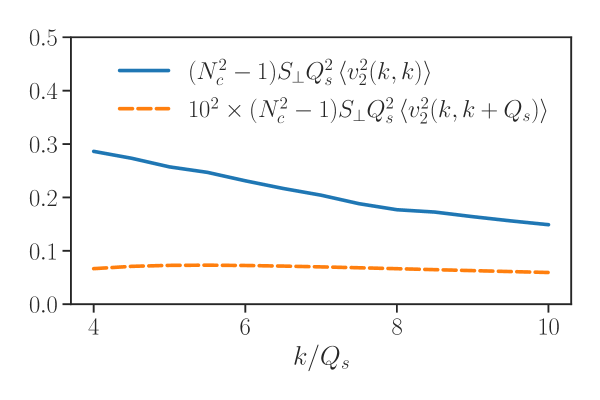
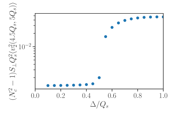
Figure 1: Left panel: The second flow harmonic, $v_{2}^{2}$ as a function of the momentum. The calculation of $v^{2}_{2}$ is performed for two cases: a) the same momentum of the pair, b) the momentum of the pair is offset by the saturation momentum of the target in order to avoid the gluon HBT effect. The bin width in both cases is $\Delta=Q_{s}/2$.
Right panel: The second flow harmonic, $v_{2}^{2}$ as a function of the bin width. The centers of the two bins are chosen at $k=4.5Q_{s}$, $k^{\prime}=5Q_{s}$.

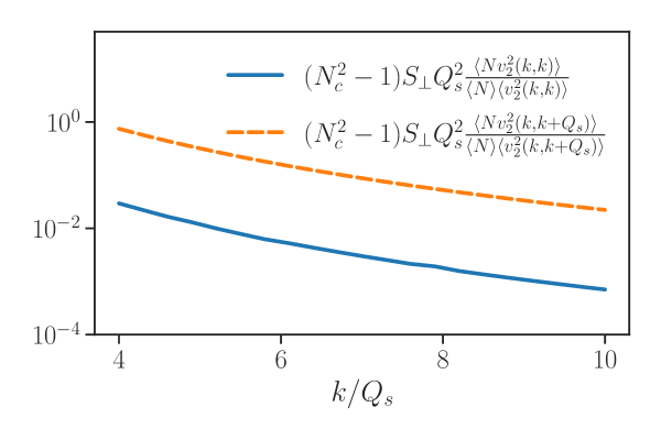
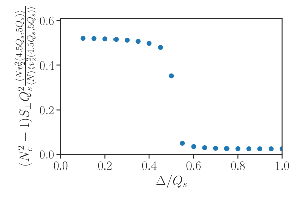
Figure 2: Left panel: The three particle correlation function ${\cal O}_{N,v_{2}}$ defined by the normalized correlations between $v^{2}_{2}$ and the total multiplicity of produced particles. The calculation of $v^{2}_{2}$ is performed for two cases: a) the same momentum of the pair, b) the momentum of the pair is offset by the saturation momentum of the target in order to avoid the gluon HBT effect. The bin width in both cases is $\Delta=Q_{s}/2$.
Right panel: The three particle correlation function ${\cal O}_{N,v_{2}}$ as a function of the bin width.

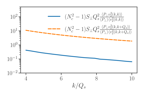
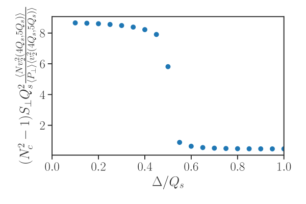
Figure 3: Left panel: The three particle correlation function ${\cal O}_{k,v_{2}}$. Kinematics is the same as in Fig. 2.
Right panel: The three particle correlation ${\cal O}_{k,v_{2}}$ as a function of bin width.

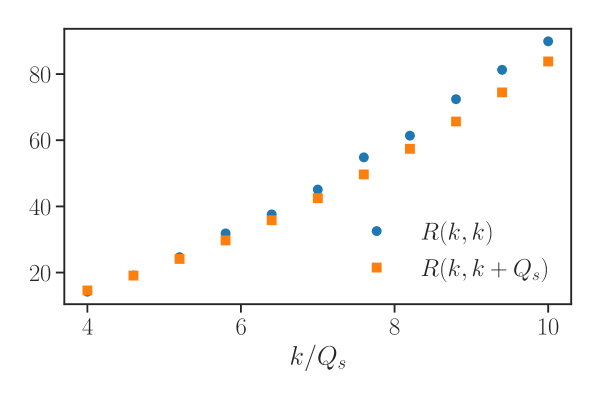
Figure 4: The ratio $R\equiv{\cal O}_{k,v_{2}}/{\cal O}_{N,v_{2}}$ as a function of transverse momentum.

V Discussion

Our results are quite curious.

First, regarding $v^{2}_{2}$ we find a very characteristic sharp transition in the value of $v^{2}_{2}$ as a function of the bin width. Referring to Fig. 1 the value of $v_{2}$ rises sharply from $v_{2}\approx 2\times 10^{-3}$ to $v_{2}\approx 1.5\times 10^{-2}$, i.e. almost by an order of magnitude as the bin width is increased from $\Delta<|k-k^{\prime}|$ to $\Delta>|k-k^{\prime}|$. This transition is entirely due to the fact that at this value of bin width the HBT correlations start contributing to the second flow harmonic, since the HBT peak is much narrower than the Bose correlation. Although the presence of the transition is expected on these grounds, the fact that the value of $v_{2}$ rises by such a large amount is worth noting. We conclude that the contribution of the HBT correlations to $v_{2}$ completely overwhelms the contribution of Bose enhancement. The actual numerical value for $v_{2}$ that we get is quite reasonable. For bins centered at $k=4.5Q_{s}\approx 4.5$ GeV and $k^{\prime}=5Q_{s}\approx 5$ GeV and $\Delta=Q_{s}$ (right panel in Fig. 1) we find $v_{2}\approx 1.5\times 10^{-2}$. This is to be compared to typical values of $0.05\ -\ 0.08$ for transverse momentum integrated $v_{2}$ in p-Pb collisions at LHC ridge . Since the integrated $v_{2}$ is dominated by the lower momenta, this discrepancy of a factor of $5$ or so may be attributable to the relatively high value of transverse momentum in our calculation. The trend of $v_{2}$ rising towards low momenta is clearly seen in the left panel of Fig. 1.

We do reiterate though, that our calculation is not meant as a phenomenological fit in any way, but rather as a qualitative study of the effects of quantum statistics on the correlations. As such, we note that the sharp rise in $v_{2}$ with bin width is a very characteristic behavior, and it would be very interesting to explore such dependence experimentally.

We wish to comment on two peculiar features seen on the left panel in Fig. 1. First, it is interesting to note that in the regime dominated by Bose correlations (dashed curve), $v^{2}_{2}$ is only very weakly dependent on the transverse momentum. Although it does slowly decrease towards large momenta, this decrease cannot be discerned for the range of momenta on the plot. This suggests that the Bose correlated part of the two particle production scales with the same power of momentum as the square of the single particle spectrum.

Another property to note is that the ratio of the HBT to Bose contributions as seen in the left panel of Fig. 1 seems to be even greater than on the right panel. The ratio between the solid and dashed curves at $k\sim 4-5Q_{s}$ on the left panel is around $\sim 500$, rather than the factor $\sim 50$ that we have inferred from the right panel. Admittedly, it is not a completely fair comparison, as the solid line on the left panel corresponds to the two momenta sampled from the same bin, while on the right panel the centers of the two bins are displaced by $0.5Q_{s}$. Still it is a little surprising that a relatively small displacement of the bin centers leads to such a dramatic effect. The reason for this is our treatment of the projectile as translationally invariant, which leads to a delta-function HBT correlation. In this situation the HBT contribution is essentially given by the overlap area of two rings corresponding to the two momentum bins. Displacing the centers of the bins relative to each other even by a small amount leads to a significant change of the overlap area, and thus the HBT contribution has a sharp peak at zero displacement. As we mentioned before, in a more realistic treatment which takes into account finite transverse size of the proton, the HBT peak should be smeared to have a width $\sim 0.2$ GeV (the inverse radius of the projectile) which should significantly soften the dependence on $|k-k^{\prime}|$. We have checked numerically that smearing the HBT peak does indeed have such an effect. For that reason we limit our consideration to kinematic situations where the distance between the bin centers is greater than $0.3-0.4Q_{s}$.

Moving on to the correlation of $v^{2}_{2}$ with multiplicity as well as with the transverse momentum, we again observe a very characteristic dependence on the bin width. For small bin width where the HBT does not contribute, the correlation is sizable, $\sim 3\times 10^{-3}$. However for larger bin width this correlation drops by a factor of about $30$ to $50$, and is negligible. Note that the transition in ${\cal O}_{N,v_{2}}$ and ${\cal O}_{k,v_{2}}$ is the opposite to that in $v_{2}$: whereas $v_{2}$ is smaller at small $\Delta$, the correlations ${\cal O}_{N,v_{2}}$ and ${\cal O}_{k,v_{2}}$ are larger, and vice versa. This tells us that although the contribution of HBT to $v_{2}$ is much larger than that of the Bose enhancement, the HBT is much weaker correlated with total multiplicity (and transverse momentum) than the Bose enhancement is. In fact, since the magnitude of the drop in Fig. 2 is about the same as the magnitude of the rise in Fig. 1, we conclude that the numerator in Eq. (III.2) is a rather smooth function of $\Delta$, and the drop in Fig. 2 is driven entirely by the sharp rise in the denominator in Eq. (III.2) (and the same is true for Eq. (56)).

The correlation between $v_{2}$ and $N$ is a decreasing function of momentum. This is easy to understand, since the multiplicity is dominated by soft particles, while the correlation we track originates with gluons that already in the incoming wave function have large transverse momentum. We thus have no reason to expect a correlation at high values of $k$. Another aspect of this is seen in Fig. 4 which shows that the correlation of $v_{2}$ with $k$ remains larger at high momentum than the correlation of $v_{2}$ with $N$, since particles with higher momentum contribute more significantly to average momentum than to the total multiplicity.

Qualitatively the smallness of the correlations between $v_{2}$ and $N$ is consistent with the experimental data ridge . Experimentally the change in the integrated $v_{2}$ in p-Pb collisions is at most $40\%$ over an order of magnitude change in $N$. Again, we note that our calculation is valid only for large $k$. The correlation clearly grows towards smaller values of $k$, but within our approximation we cannot push much below $k\sim 4Q_{s}$.

To conclude, we have calculated $v_{2}$ and correlations of $v_{2}$ with the total multiplicity and average transverse momentum per particle in the dense-dilute CGC approach using the GBW model for dipole amplitude. Our results are valid at large $N_{c}$ and large transverse momentum. We have not made an attempt to include any additional effects beyond multiple scattering in our calculation. We find a reasonable magnitude for $v_{2}$ and very small correlations with total multiplicity, consistent with data. An interesting observation we make is a characteristic very strong crossover in $v_{2}(k,k^{\prime},\Delta)$ as a function of the width of the transverse momentum bin $\Delta$ at fixed $k$ and $k^{\prime}$, associated with the dominance of the HBT contribution. It would be very interesting to explore such a dependence experimentally.

VI Appendix

VI.1 Computation of $X_{i}$ for the correlations between multiplicity and $v_{2}$

VI.1.1 Computation of $X_{1}$

Consider $X_{1}$ first. The $k_{1}$ integral is facilitated by Eq. (15):

$$\int d^{2}k_{1}\frac{dN^{(3)}}{d^{2}k_{1}\,d^{2}k_{2}\,d^{2}k_{3}}\bigg{|}_{X,1}=\big{[}(X_{1,a}+X_{1,b})+(k_{3}\to-k_{3})\big{]}+\big{[}(X_{1,c}+X_{1,d})+(k_{1}\to-k_{1})\big{]},$$ (68)

where $X_{1,a}$ is the first term in Eq. (30), $X_{1,b}$ is the second term in Eq. (30), $X_{1,c}$ is the first term in Eq. (31) and $X_{1,d}$ is the second term in Eq. (31), all integrated over $k_{1}$. The explicit expression of $X_{1,a}$ reads

$$X_{1,a} = \alpha_{s}^{3}(4\pi)^{3}(N_{c}^{2}-1)\,\mu^{6}\,(2\pi)^{6}\int d^{2}k_{1}\,\frac{d^{2}q_{1}}{(2\pi)^{2}}\,\frac{d^{2}q_{2}}{(2\pi)^{2}}\,\frac{d^{2}q_{3}}{(2\pi)^{2}}\,d(q_{1})\,d(q_{2})\,d(q_{3})$$ (69)

$$\times \delta^{(2)}(k_{1}-k_{2})\,\delta^{(2)}(k_{1}-q_{1}+q_{3}-k_{3})\,\delta^{(2)}(k_{3}-q_{3}+q_{1}-k_{2})$$

$$\times L^{i}(k_{1},q_{1})L^{i}(k_{1},q_{2})\,L^{j}(k_{2},q_{2})L^{j}(k_{2},q_{1})\,L^{k}(k_{3},q_{3})L^{k}(k_{3},q_{3}).$$

We use the first $\delta$-function to integrate over $k_{1}$, the second $\delta$-function to integrate over $q_{1}$, and the third $\delta$-function becomes $\delta(0)$ which, as usual, is regulated by the transverse area $S_{\perp}$ of the projectile. The result reads

$$X_{1,a} = \alpha_{s}^{3}(4\pi)^{3}(N_{c}^{2}-1)\,\mu^{6}\,(2\pi)^{2}\,S_{\perp}\int\frac{d^{2}q_{2}}{(2\pi)^{2}}\,\frac{d^{2}q_{3}}{(2\pi)^{2}}\,d\big{[}k_{2}-(k_{3}-q_{3})\big{]}\,d(q_{2})\,d(q_{3})\,\bigg{[}\frac{(k_{3}-q_{3})^{i}}{(k_{3}-q_{3})^{2}}-\frac{k_{2}^{i}}{k_{2}^{2}}\bigg{]}$$ (70)

$$\times \bigg{[}\frac{(k_{2}-q_{2})^{i}}{(k_{2}-q_{2})^{2}}-\frac{k_{2}^{i}}{k_{2}^{2}}\bigg{]}\bigg{[}\frac{(k_{2}-q_{2})^{j}}{(k_{2}-q_{2})^{2}}-\frac{k_{2}^{j}}{k_{2}^{2}}\bigg{]}\bigg{[}\frac{(k_{3}-q_{3})^{j}}{(k_{3}-q_{3})^{2}}-\frac{k_{2}^{j}}{k^{2}_{2}}\bigg{]}\;\bigg{[}\frac{(k_{3}-q_{3})^{k}}{(k_{3}-q_{3})^{2}}-\frac{k_{3}^{k}}{k_{3}^{2}}\bigg{]}\bigg{[}\frac{(k_{3}-q_{3})^{k}}{(k_{3}-q_{3})^{2}}-\frac{k_{3}^{k}}{k_{3}^{2}}\bigg{]}.$$

Note that the dipole $d\big{[}k_{2}-(k_{3}-q_{3})\big{]}$ is enhanced when its argument is small. Hence $X_{1,a}$ is a contribution to the forward ($k_{2}\simeq k_{3}$) correlation of gluons $2$ and $3$.

The rest of the terms in $X_{1}$ can be computed in a similar way:

$$X_{1,b} = \alpha_{s}^{3}(4\pi)^{3}(N_{c}^{2}-1)\,\mu^{6}\,(2\pi)^{2}\,S_{\perp}\int\frac{d^{2}q_{2}}{(2\pi)^{2}}\,\frac{d^{2}q_{3}}{(2\pi)^{2}}\,d\big{[}k_{2}+(k_{3}-q_{3})\big{]}\,d(q_{2})\,d(q_{3})\,\bigg{[}\frac{(k_{3}-q_{3})^{i}}{(k_{3}-q_{3})^{2}}+\frac{k_{2}^{i}}{k_{2}^{2}}\bigg{]}$$ (71)

$$\times \bigg{[}\frac{(k_{2}+q_{2})^{i}}{(k_{2}+q_{2})^{2}}-\frac{k_{2}^{i}}{k_{2}^{2}}\bigg{]}\bigg{[}\frac{(k_{3}-q_{3})^{j}}{(k_{2}-q_{2})^{2}}+\frac{k_{2}^{j}}{k_{2}^{2}}\bigg{]}\bigg{[}\frac{(k_{2}+q_{2})^{j}}{(k_{2}+q_{2})^{2}}-\frac{k_{2}^{j}}{k^{2}_{2}}\bigg{]}\;\bigg{[}\frac{(k_{3}-q_{3})^{k}}{(k_{3}-q_{3})^{2}}-\frac{k_{3}^{k}}{k_{3}^{2}}\bigg{]}\bigg{[}\frac{(k_{3}-q_{3})^{k}}{(k_{3}-q_{3})^{2}}-\frac{k_{3}^{k}}{k_{3}^{2}}\bigg{]}.$$

$X_{1,b}$ is a contribution to the backward correlation of gluons $2$ and $3$. By renaming $q_{2}\to-q_{2}$ and $q_{3}\to-q_{3}$, it is easy to see that $X_{1,b}=X_{1,a}(k_{3}\to-k_{3})$.

$$X_{1,c} = \alpha_{s}^{3}(4\pi)^{3}(N_{c}^{2}-1)\,\mu^{6}\,(2\pi)^{2}\,S_{\perp}\int\frac{d^{2}q_{2}}{(2\pi)^{2}}\,\frac{d^{2}q_{3}}{(2\pi)^{2}}\,d\big{[}k_{2}+(k_{3}-q_{3})\big{]}\,d(q_{2})\,d(q_{3})\,\bigg{[}\frac{(k_{3}-q_{3})^{i}}{(k_{3}-q_{3})^{2}}+\frac{k_{2}^{i}}{k_{2}^{2}}\bigg{]}$$ (72)

$$\times \bigg{[}\frac{(k_{2}-q_{2})^{i}}{(k_{2}-q_{2})^{2}}-\frac{k_{2}^{i}}{k_{2}^{2}}\bigg{]}\bigg{[}\frac{(k_{3}-q_{3})^{j}}{(k_{3}-q_{3})^{2}}+\frac{k_{2}^{j}}{k_{2}^{2}}\bigg{]}\bigg{[}\frac{(k_{2}-q_{2})^{j}}{(k_{2}-q_{2})^{2}}-\frac{k_{2}^{j}}{k_{2}^{2}}\bigg{]}\;\bigg{[}\frac{(k_{3}-q_{3})^{k}}{(k_{3}-q_{3})^{2}}-\frac{k_{3}^{k}}{k_{3}^{2}}\bigg{]}\bigg{[}\frac{(k_{3}-q_{3})^{k}}{(k_{3}-q_{3})^{2}}-\frac{k_{3}^{k}}{k_{3}^{2}}\bigg{]}.$$

$X_{1,c}$ is a contribution to the backward correlation of gluons $2$ and $3$. By renaming $q_{3}\to-q_{3}$, it is easy to show that $X_{1,c}=X_{1,a}(k_{3}\to-k_{3})$.

$$X_{1,d} = \alpha_{s}^{3}(4\pi)^{3}(N_{c}^{2}-1)\,\mu^{6}\,(2\pi)^{2}\,S_{\perp}\int\frac{d^{2}q_{2}}{(2\pi)^{2}}\,\frac{d^{2}q_{3}}{(2\pi)^{2}}\,d\big{[}k_{2}-(k_{3}-q_{3})\big{]}\,d(q_{2})\,d(q_{3})\,\bigg{[}\frac{(k_{3}-q_{3})^{i}}{(k_{3}-q_{3})^{2}}-\frac{k_{2}^{i}}{k_{2}^{2}}\bigg{]}$$ (73)

$$\times \bigg{[}\frac{(k_{2}-q_{2})^{i}}{(k_{2}-q_{2})^{2}}-\frac{k_{2}^{i}}{k_{2}^{2}}\bigg{]}\bigg{[}\frac{(k_{3}-q_{3})^{j}}{(k_{3}-q_{3})^{2}}-\frac{k_{2}^{j}}{k_{2}^{2}}\bigg{]}\bigg{[}\frac{(k_{2}-q_{2})^{j}}{(k_{2}-q_{2})^{2}}-\frac{k_{2}^{j}}{k_{2}^{2}}\bigg{]}\;\bigg{[}\frac{(k_{3}-q_{3})^{k}}{(k_{3}-q_{3})^{2}}-\frac{k_{3}^{k}}{k_{3}^{2}}\bigg{]}\bigg{[}\frac{(k_{3}-q_{3})^{k}}{(k_{3}-q_{3})^{2}}-\frac{k_{3}^{k}}{k_{3}^{2}}\bigg{]}.$$

$X_{1,d}$ is a contribution to the forward correlation of gluons $2$ and $3$. $X_{1,d}=X_{1,a}$.

Combining all the terms, we get

$$X_{1}=4\,\alpha_{s}^{3}(4\pi)^{3}(N_{c}^{2}-1)\,\mu^{6}\,(2\pi)^{2}\,S_{\perp}\int\frac{d^{2}q_{2}}{(2\pi)^{2}}\,\frac{d^{2}q_{3}}{(2\pi)^{2}}\bigg{\{}d\big{[}k_{2}-(k_{3}-q_{3})\big{]}\,d(q_{2})\,d(q_{3})\,\bigg{[}\frac{(k_{3}-q_{3})^{i}}{(k_{3}-q_{3})^{2}}-\frac{k_{2}^{i}}{k_{2}^{2}}\bigg{]}$$

$$\times \bigg{[}\frac{(k_{2}-q_{2})^{i}}{(k_{2}-q_{2})^{2}}-\frac{k_{2}^{i}}{k_{2}^{2}}\bigg{]}\bigg{[}\frac{(k_{3}-q_{3})^{j}}{(k_{3}-q_{3})^{2}}-\frac{k_{2}^{j}}{k_{2}^{2}}\bigg{]}\bigg{[}\frac{(k_{2}-q_{2})^{j}}{(k_{2}-q_{2})^{2}}-\frac{k_{2}^{j}}{k_{2}^{2}}\bigg{]}\;\bigg{[}\frac{(k_{3}-q_{3})^{k}}{(k_{3}-q_{3})^{2}}-\frac{k_{3}^{k}}{k_{3}^{2}}\bigg{]}\bigg{[}\frac{(k_{3}-q_{3})^{k}}{(k_{3}-q_{3})^{2}}-\frac{k_{3}^{k}}{k_{3}^{2}}\bigg{]}+(k_{3}\to-k_{3})\bigg{\}}.$$

In $X_{1}$, the first term is a contribution to the forward correlation of the gluons 2 and 3. The second term with $(k_{3}\to-k_{3})$ is a contribution to the backward correlation of the gluons 2 and 3. Shifting and renaming the variables the expression can be brought to a more compact form:

$$X_{1} \equiv 4\,\alpha_{s}^{3}(4\pi)^{3}(N_{c}^{2}-1)\,\mu^{6}(2\pi)^{2}\,S_{\perp}\,\int\frac{d^{2}q_{2}}{(2\pi)^{2}}\frac{d^{2}q_{3}}{(2\pi)^{2}}\,\bigg{\{}d(q_{2}+k_{2})\,d(q_{3}+k_{2})\,d(q_{3}+k_{3})$$

$$\hskip 71.13188pt\times\bigg{[}\frac{q^{i}_{2}}{q_{2}^{2}}+\frac{k^{i}_{2}}{k_{2}^{2}}\bigg{]}\bigg{[}\frac{q^{j}_{2}}{q_{2}^{2}}+\frac{k^{j}_{2}}{k_{2}^{2}}\bigg{]}\bigg{[}\frac{q^{i}_{3}}{q_{3}^{2}}+\frac{k^{i}_{2}}{k_{2}^{2}}\bigg{]}\bigg{[}\frac{q^{j}_{3}}{q_{3}^{2}}+\frac{k^{j}_{2}}{k_{2}^{2}}\bigg{]}\bigg{[}\frac{q^{k}_{3}}{q_{3}^{2}}+\frac{k^{k}_{3}}{k_{3}^{2}}\bigg{]}\bigg{[}\frac{q^{k}_{3}}{q_{3}^{2}}+\frac{k^{k}_{3}}{k_{3}^{2}}\bigg{]}+(k_{3}\to-k_{3})\bigg{\}}.$$

Using the GBW model (20) for the dipoles $d$, the $X_{1}$ contribution can be written as

$$X_{1} = 4\,\alpha_{s}^{3}(4\pi)^{3}(N_{c}^{2}-1)\,\mu^{6}\,(2\pi)^{2}\,S_{\perp}\,\frac{1}{(2\pi)^{4}}\,\bigg{(}\frac{4\pi}{Q_{s}^{2}}\bigg{)}^{3}\,e^{-(2k_{2}^{2}+k_{3}^{2})/Q_{s}^{2}}$$ (76)

$$\times \int d^{2}q_{2}\,e^{-(q_{2}^{2}+2\,q_{2}\cdot k_{2})/Q_{s}^{2}}\bigg{[}\frac{k_{2}^{i}}{k_{2}^{2}}\frac{k_{2}^{j}}{k_{2}^{2}}+\frac{k_{2}^{i}}{k_{2}^{2}}\frac{q_{2}^{j}}{q_{2}^{2}}+\frac{q_{2}^{i}}{q_{2}^{2}}\frac{k_{2}^{j}}{k_{2}^{2}}+\frac{q_{2}^{i}}{q_{2}^{2}}\frac{q_{2}^{j}}{q_{2}^{2}}\bigg{]}$$

$$\times \int d^{2}q_{3}\,e^{-[2q_{3}^{2}+2q_{3}\cdot(k_{2}+k_{3})]/Q_{s}^{2}}\bigg{[}\frac{k_{2}^{i}}{k_{2}^{2}}\frac{k_{2}^{j}}{k_{2}^{2}}+\frac{k_{2}^{i}}{k_{2}^{2}}\frac{q_{3}^{j}}{q_{3}^{2}}+\frac{q_{3}^{i}}{q_{3}^{2}}\frac{k_{2}^{j}}{k_{2}^{2}}+\frac{q_{3}^{i}}{q_{3}^{2}}\frac{q_{3}^{j}}{q_{3}^{2}}\bigg{]}\bigg{[}\frac{1}{q_{3}^{2}}+2\,\frac{q_{3}^{k}}{q_{3}^{2}}\frac{k_{3}^{k}}{k_{3}^{2}}+\frac{1}{k_{3}^{2}}\bigg{]}.$$

Note that $X_{1}\propto e^{-(2k_{2}^{2}+k_{3}^{2})/Q_{s}^{2}}$ which provides an exponential suppression for produced gluon momenta much larger than the target saturation scale $Q_{s}$. However we still have the $q_{2}$ and $q_{3}$ integrations to perform, and those may bring a compensating exponential enhancement. Next, we will perform these integrations concentrating on such possible enhancing factors. Let us first focus on the $q_{2}$ integration (the $q_{3}$ integration is done similarly and will follow). There are three types of Gaussian integrals to consider:

$$I_{0,0} = \int d^{2}q_{2}\,e^{-(q_{2}^{2}+2\,q_{2}\cdot k_{2})/Q_{s}^{2}}\ ,$$ (77)

$$I^{i}_{1,2} = \int d^{2}q_{2}\,e^{-(q_{2}^{2}+2\,q_{2}\cdot k_{2})/Q_{s}^{2}}\,\frac{q_{2}^{i}}{q_{2}^{2}}\ ,$$

$$I_{2,4}^{ij} = \int d^{2}q_{2}\,e^{-(q_{2}^{2}+2\,q_{2}\cdot k_{2})/Q_{s}^{2}}\,\frac{q_{2}^{i}}{q_{2}^{2}}\frac{q_{2}^{j}}{q_{2}^{2}}\ .$$

The first integral is trivial,

$$I_{0,0}=\pi Q_{s}^{2}\;e^{k_{2}^{2}/Q_{s}^{2}}.$$ (78)

The second and the third integrals are performed with the help of a Schwinger parameter $t$ introduced for the $q_{2}^{2}$ factor in the denominator:

$$I_{1,2}^{i} = \int_{0}^{+\infty}dt\exp\bigg{[}\frac{k_{2}^{2}}{Q_{s}^{2}(1+Q_{s}^{2}t)}\bigg{]}\int d^{2}q\exp\bigg{[}-\frac{(1+Q_{s}^{2}t)}{Q_{s}^{2}}q^{2}\bigg{]}\bigg{[}q^{i}-\frac{k_{2}^{i}}{(1+Q_{s}^{2}t)}\bigg{]}$$ (79)

$$= -\pi Q_{s}^{2}\,k_{2}^{i}\int_{0}^{+\infty}dt\frac{1}{(1+Q_{s}^{2}t)^{2}}\,\exp\bigg{[}\frac{k_{2}^{2}}{Q_{s}^{2}(1+Q_{s}^{2}t)}\bigg{]}.$$

Changing variables to $t^{\prime}=1/(1+Q_{s}^{2}t)$, the result reads

$$I_{1,2}^{i} = -\pi Q_{s}^{2}\,k_{2}^{i}\frac{1}{Q_{s}^{2}}\int_{0}^{1}dt^{\prime}\,e^{k_{2}^{2}t^{\prime}/Q_{s}^{2}}=\pi Q_{s}^{2}\,\frac{k_{2}^{i}}{k_{2}^{2}}\Big{(}1-e^{k_{2}^{2}/Q_{s}^{2}}\Big{)}.$$ (80)

For the last integration, $I_{2,4}$, a similar procedure is followed, but with two Schwinger parameters $t_{1}$ and $t_{2}$ for each $1/q_{2}^{2}$ factor. This makes it possible to perform the integration over $q_{2}$ and one of the Schwinger parameters. However, the remaining integral over the second Schwinger parameter is divergent, reflecting the original IR divergence of the $q_{2}$ integration. The origin of this IR divergence is pretty clear - it is an artefact of the approximation (15) with momentum independent $\mu$. In fact, color neutrality should be imposed at some non-perturbative IR scale $\Lambda_{min}$ below which $\mu$ must vanish, $\mu(p<\Lambda_{min})=0$. Roughly $\Lambda^{2}_{min}\sim 1/S_{\perp}$. We find it more convenient introducing a cutoff $\lambda\rightarrow 0$ on the Schwinger parameter than the sharp IR cutoff $\Lambda_{min}$ to regulate this divergence. The relation between the two is

$$\lambda\simeq\Lambda^{2}_{min}/Q_{s}^{2}\simeq 1/(S_{\perp}Q_{s}^{2}).$$ (81)

The final result reads

$$I_{2,4}^{ij} = \pi Q_{s}^{2}\,\bigg{\{}\frac{\delta^{ij}}{2}\bigg{\lgroup}\frac{1}{Q_{s}^{2}}+\frac{1}{k_{2}^{2}}\Big{(}1-e^{k^{2}_{2}/Q_{s}^{2}}\Big{)}+\frac{1}{Q_{s}^{2}}\bigg{[}{\rm Ei}\bigg{(}\frac{k_{2}^{2}}{Q_{s}^{2}}\bigg{)}-{\rm Ei}\bigg{(}\frac{k_{2}^{2}\,\lambda}{Q_{s}^{2}}\bigg{)}\bigg{]}\bigg{\rgroup}-\frac{k_{2}^{i}}{k_{2}^{2}}\frac{k_{2}^{j}}{k_{2}^{2}}\bigg{\lgroup}\frac{k_{2}^{2}}{Q_{s}^{2}}+\Big{(}1-e^{k_{2}^{2}/Q_{s}^{2}}\Big{)}\bigg{\rgroup}\bigg{\}},$$ (82)

where ${\rm Ei}$ is an exponential integral special function. Combining the results given in Eqs. (78), (80) and (82), the overall result of the $q_{2}$ integration reads

$$\int d^{2}q_{2}\,e^{-(q_{2}^{2}+2\,q_{2}\cdot k_{2})/Q_{s}^{2}}\bigg{[}\frac{k_{2}^{i}}{k_{2}^{2}}\frac{k_{2}^{j}}{k_{2}^{2}}+\frac{k_{2}^{i}}{k_{2}^{2}}\frac{q_{2}^{j}}{q_{2}^{2}}+\frac{q_{2}^{i}}{q_{2}^{2}}\frac{k_{2}^{j}}{k_{2}^{2}}+\frac{q_{2}^{i}}{q_{2}^{2}}\frac{q_{2}^{j}}{q_{2}^{2}}\bigg{]}$$ (83)

$$\hskip 56.9055pt=\pi Q_{s}^{2}\,\bigg{\{}\frac{k_{2}^{i}}{k_{2}^{2}}\frac{k_{2}^{j}}{k_{2}^{2}}\bigg{(}1-\frac{k_{2}^{2}}{Q_{s}^{2}}\bigg{)}+\frac{\delta^{ij}}{2}\frac{1}{k_{2}^{2}}\bigg{\lgroup}\frac{k_{2}^{2}}{Q_{s}^{2}}+\Big{(}1-e^{k_{2}^{2}/Q_{s}^{2}}\Big{)}+\frac{k_{2}^{2}}{Q_{s}^{2}}\bigg{[}{\rm Ei}\bigg{(}\frac{k_{2}^{2}}{Q_{s}^{2}}\bigg{)}-{\rm Ei}\bigg{(}\frac{k_{2}^{2}\,\lambda}{Q_{s}^{2}}\bigg{)}\bigg{]}\bigg{\rgroup}\bigg{\}}.$$

So far the integration over $q_{2}$ was computed without any approximation. Yet, as we have mentioned above, we are interested only in terms in $X_{1}$ that are not exponentially suppressed. In other words, only exponentially enhanced terms in (83) are of interest. The $\lambda$-dependent terms are not of that type and can be neglected. For $k_{2}^{2}\gg Q_{s}^{2}$, the result can be simplified using the large argument asymptotic expansion of the exponential integral function,

$${\rm Ei}(x)\approx\frac{e^{x}}{x}\bigg{(}1+\frac{1!}{x}+\frac{2!}{x^{2}}+\frac{3!}{x^{3}}+\cdots\bigg{)},\ \ x\rightarrow\infty.$$ (84)

Thus the exponentially enhanced contribution to the total $q_{2}$ integral reads

$$\int d^{2}q_{2}\,e^{-(q_{2}^{2}+2\,q_{2}\cdot k_{2})/Q_{s}^{2}}\bigg{[}\frac{k_{2}^{i}}{k_{2}^{2}}\frac{k_{2}^{j}}{k_{2}^{2}}+\frac{k_{2}^{i}}{k_{2}^{2}}\frac{q_{2}^{j}}{q_{2}^{2}}+\frac{q_{2}^{i}}{q_{2}^{2}}\frac{k_{2}^{j}}{k_{2}^{2}}+\frac{q_{2}^{i}}{q_{2}^{2}}\frac{q_{2}^{j}}{q_{2}^{2}}\bigg{]}\approx\pi Q_{s}^{2}\;e^{k_{2}^{2}/Q_{s}^{2}}\;\frac{\delta^{ij}}{2}\frac{Q_{s}^{2}}{k_{2}^{4}}\;\bigg{(}1+\frac{2!\,Q_{s}^{2}}{k_{2}^{2}}+\frac{3!\,Q_{s}^{4}}{k_{2}^{4}}\bigg{)}.$$ (85)

We have kept sub-leading terms of the order $Q_{s}^{4}/k_{2}^{4}$ since, as we will see later, those will turn out to be the first non-vanishing terms when $k_{2}=k_{3}$. After the $q_{2}$ integration has been evaluated, $X_{1}$ still contains a $q_{3}$ integral, which is our next target:

$$X_{1} \approx \alpha_{s}^{3}(4\pi)^{3}(N_{c}^{2}-1)\;\mu^{6}\;S_{\perp}\;\frac{1}{(2\pi)}\,\frac{(4\pi)^{3}}{Q_{s}^{2}}\;e^{-(k_{2}^{2}+k_{3}^{2})/Q_{s}^{2}}\,\frac{1}{k_{2}^{4}}\;\bigg{(}1+\frac{2!\,Q_{s}^{2}}{k_{2}^{2}}+\frac{3!\,Q_{s}^{4}}{k_{2}^{4}}\bigg{)}$$

$$\times \int d^{2}q_{3}\,e^{-[2q_{3}^{2}+2q_{3}\cdot(k_{2}+k_{3})]/Q_{s}^{2}}\bigg{[}\frac{1}{k_{2}^{2}}+2\frac{k_{2}^{i}}{k_{2}^{2}}\frac{q_{3}^{i}}{q_{3}^{2}}+\frac{1}{q_{3}^{2}}\bigg{]}\bigg{[}\frac{1}{q_{3}^{2}}+2\,\frac{q_{3}^{j}}{q_{3}^{2}}\frac{k_{3}^{j}}{k_{3}^{2}}+\frac{1}{k_{3}^{2}}\bigg{]}$$

$$\approx \alpha_{s}^{3}(4\pi)^{3}(N_{c}^{2}-1)\;\mu^{6}\;S_{\perp}\;\frac{1}{(2\pi)}\,\frac{(4\pi)^{3}}{Q_{s}^{2}}\;e^{-(k_{2}^{2}+k_{3}^{2})/Q_{s}^{2}}\,\frac{1}{k_{2}^{4}}\;\bigg{(}1+\frac{2!\,Q_{s}^{2}}{k_{2}^{2}}+\frac{3!\,Q_{s}^{4}}{k_{2}^{4}}\bigg{)}$$

$$\times \;\bigg{\{}\frac{1}{k_{2}^{2}k_{3}^{2}}T_{0,0}+\bigg{(}\frac{1}{k_{2}^{2}}+\frac{1}{k_{3}^{2}}\bigg{)}T_{0,2}+T_{0,4}+\frac{2(k_{2}+k_{3})^{i}}{k_{2}^{2}k_{3}^{2}}T^{i}_{1,2}+2\bigg{(}\frac{k_{2}^{i}}{k_{2}^{2}}+\frac{k_{3}^{i}}{k_{3}^{2}}\bigg{)}T^{i}_{1,4}+4\frac{k_{2}^{i}}{k_{2}^{2}}\frac{k_{3}^{i}}{k_{3}^{2}}T^{ij}_{2,4}\bigg{\}},$$

where

$$T_{0,0} = \int d^{2}q_{3}\,e^{-[2q_{3}^{2}+2q_{3}\cdot(k_{2}+k_{3})]/Q_{s}^{2}},$$ (87)

$$T_{0,2} = \int d^{2}q_{3}\,e^{-[2q_{3}^{2}+2q_{3}\cdot(k_{2}+k_{3})]/Q_{s}^{2}}\frac{1}{q_{3}^{2}}\ ,$$ (88)

$$T_{0,4} = \int d^{2}q_{3}\,e^{-[2q_{3}^{2}+2q_{3}\cdot(k_{2}+k_{3})]/Q_{s}^{2}}\frac{1}{q_{3}^{4}}\ ,$$ (89)

$$T^{i}_{1,2} = \int d^{2}q_{3}\,e^{-[2q_{3}^{2}+2q_{3}\cdot(k_{2}+k_{3})]/Q_{s}^{2}}\frac{q_{3}^{i}}{q_{3}^{2}}\ ,$$ (90)

$$T^{i}_{1,4} = \int d^{2}q_{3}\,e^{-[2q_{3}^{2}+2q_{3}\cdot(k_{2}+k_{3})]/Q_{s}^{2}}\frac{q_{3}^{i}}{q_{3}^{4}}\ ,$$ (91)

$$T^{ij}_{2,4} = \int d^{2}q_{3}\,e^{-[2q_{3}^{2}+2q_{3}\cdot(k_{2}+k_{3})]/Q_{s}^{2}}\frac{q_{3}^{i}q_{3}^{j}}{q_{3}^{4}}\ .$$ (92)

The structure of these integrals over $q_{3}$ are very similar to the ones encountered in the $q_{2}$ integrations (77). Therefore, the integration over $q_{3}$ can be performed in a similar manner. Again, keeping only the exponentially enhanced terms, the results read:

$$T_{0,0} = \pi Q_{s}^{2}\;e^{(k_{2}+k_{3})^{2}/2Q_{s}^{2}}\;\frac{1}{2}\ ,$$ (93)

$$T_{0,2} \approx \pi Q_{s}^{2}\;e^{(k_{2}+k_{3})^{2}/2Q_{s}^{2}}\;\frac{2^{2}}{(k_{2}+k_{3})^{2}}\bigg{[}\frac{1}{2}+\frac{1}{4}\frac{2^{2}\,Q_{s}^{2}}{(k_{2}+k_{3})^{2}}+\frac{1}{4}\frac{2^{4}\,Q_{s}^{4}}{(k_{2}+k_{3})^{4}}\bigg{]},$$ (94)

$$T_{0,4} \approx \pi Q_{s}^{2}\;e^{(k_{2}+k_{3})^{2}/2Q_{s}^{2}}\;\frac{2^{4}}{(k_{2}+k_{3})^{4}}\,\bigg{[}\frac{1}{2}+\frac{2^{2}\,Q_{s}^{2}}{(k_{2}+k_{3})^{2}}+\frac{9}{4}\frac{2^{4}\,Q_{s}^{4}}{(k_{2}+k_{3})^{4}}\bigg{]},$$ (95)

$$T^{i}_{1,2} \approx -\pi Q_{s}^{2}\>e^{(k_{2}+k_{3})^{2}/2Q_{s}^{2}}\;\frac{(k_{2}+k_{3})^{i}}{(k_{2}+k_{3})^{2}}\ ,$$ (96)

$$T^{i}_{1,4} \approx -\pi Q_{s}^{2}\>e^{(k_{2}+k_{3})^{2}/2Q_{s}^{2}}\;\frac{(k_{2}+k_{3})^{i}}{(k_{2}+k_{3})^{2}}\,\frac{2^{2}}{(k_{2}+k_{3})^{2}}\,\bigg{[}1+\frac{2^{2}\,Q_{s}^{2}}{(k_{2}+k_{3})^{2}}+\frac{3}{2}\frac{2^{4}\,Q_{s}^{4}}{(k_{2}+k_{3})^{4}}\bigg{]},$$ (97)

$$T^{ij}_{2,4} \approx \pi Q_{s}^{2}\>e^{(k_{2}+k_{3})^{2}/2Q_{s}^{2}}\;\frac{2^{2}}{(k_{2}+k_{3})^{2}}\bigg{[}\frac{1}{2}\frac{(k_{2}+k_{3})^{i}(k_{2}+k_{3})^{j}}{(k_{2}+k_{3})^{2}}+\frac{\delta^{ij}}{8}\frac{2^{2}\,Q_{s}^{2}}{(k_{2}+k_{3})^{2}}\bigg{(}1+\frac{2^{2}\,Q_{s}^{2}}{(k_{2}+k_{3})^{2}}\bigg{)}\bigg{]}.$$ (98)

Finally, using these results in Eq. (VI.1.1), $X_{1}$ can be written as

$$X_{1} \approx \frac{1}{2}\,\alpha_{s}^{3}(4\pi)^{6}(N_{c}^{2}-1)\;\mu^{6}\;S_{\perp}\ e^{-(k_{2}-k_{3})^{2}/2Q_{s}^{2}}\;\frac{1}{k_{2}^{4}}\bigg{[}1+\frac{2!\,Q_{s}^{2}}{k_{2}^{2}}+\frac{3!\,Q_{s}^{4}}{k_{2}^{4}}\bigg{]}\bigg{\{}\frac{1}{2}\frac{1}{k_{2}^{2}k_{3}^{2}}\frac{(k_{2}-k_{3})^{4}}{(k_{2}+k_{3})^{4}}$$

$$+ \frac{2^{2}\,Q_{s}^{2}}{(k_{2}+k_{3})^{2}}\frac{1}{k_{2}^{2}k_{3}^{2}}\frac{(k_{2}-k_{3})^{4}}{(k_{2}+k_{3})^{4}}+\frac{2^{4}\,Q_{s}^{4}}{(k_{2}+k_{3})^{4}}\bigg{\lgroup}\frac{1}{k_{2}^{2}k_{3}^{2}}\frac{(k_{2}-k_{3})^{4}}{(k_{2}+k_{3})^{4}}+\frac{2^{2}}{(k_{2}+k_{3})^{4}}\bigg{[}1+(k^{i}_{2}-k^{i}_{3})\bigg{(}\frac{k_{2}^{i}}{k_{2}^{2}}-\frac{k_{3}^{i}}{k_{3}^{2}}\bigg{)}\bigg{]}\bigg{\rgroup}\bigg{\}},$$

which can be organized differently and rewritten as in Eq. (49). This completes our analytical analysis of $X_{1}$.

VI.1.2 Computation of $X_{2}$

After performing the trivial integration over $k_{1}$, $X_{2}$ reads

$$X_{2}=4\,\alpha_{s}^{3}(4\pi)^{3}(N_{c}^{2}-1)\,\mu^{6}\,(2\pi)^{4}\,S_{\perp}\,\big{[}\delta^{(2)}(k_{2}-k_{3})+\delta^{(2)}(k_{2}+k_{3})\big{]}\,\int\frac{d^{2}q_{1}}{(2\pi)^{2}}\,\frac{d^{2}q_{2}}{(2\pi)^{2}}\,\frac{d^{2}q_{3}}{(2\pi)^{2}}\,d(q_{1})\,d(q_{2})\,d(q_{3})$$

$$\times\,\bigg{[}\frac{(k_{2}-q_{2})^{i}}{(k_{2}-q_{2})^{2}}-\frac{k_{2}^{i}}{k_{2}^{2}}\bigg{]}\bigg{[}\frac{(k_{2}-q_{3})^{i}}{(k_{2}-q_{3})^{2}}-\frac{k_{2}^{i}}{k_{2}^{2}}\bigg{]}\;\bigg{[}\frac{(k_{2}-q_{2})^{j}}{(k_{2}-q_{2})^{2}}-\frac{k_{2}^{j}}{k_{2}^{2}}\bigg{]}\bigg{[}\frac{(k_{2}-q_{3})^{j}}{(k_{2}-q_{3})^{2}}-\frac{k_{2}^{j}}{k_{2}^{2}}\bigg{]}$$

$$\times\,\bigg{[}\frac{(k_{2}-q_{2})^{k}}{(k_{2}-q_{2})^{2}}-\frac{(k_{2}-q_{2}+q_{1})^{k}}{(k_{2}-q_{2}+q_{1})^{2}}\bigg{]}\bigg{[}\frac{(k_{2}-q_{2})^{k}}{(k_{2}-q_{2})^{2}}-\frac{(k_{2}-q_{2}+q_{1})^{k}}{(k_{2}-q_{2}+q_{1})^{2}}\bigg{]}.$$ (100)

The first term in $X_{2}$ is an explicit contribution to the forward HBT of gluons 2 and 3. The second term, which is indeed a mirror image $(k_{3}\to-k_{3})$, is an explicit contribution to the backward HBT of gluons 2 and 3. By shifting the variables and renaming them, $X_{2}$ contribution can be put into a more compact and convenient form:

$$X_{2} \equiv 4\,\alpha_{s}^{3}(4\pi)^{3}(N_{c}^{2}-1)\,\mu^{6}\,(2\pi)^{4}\,S_{\perp}\Big{[}\delta^{(2)}(k_{2}+k_{3})+\delta^{(2)}(k_{2}-k_{3})\Big{]}\int\frac{d^{2}q_{1}}{(2\pi)^{2}}\frac{d^{2}q_{2}}{(2\pi)^{2}}\frac{d^{2}q_{3}}{(2\pi)^{2}}\,$$

$$\times d(q_{1}+q_{2})\,d(q_{2}+k_{2})\,d(q_{3}+k_{2})\bigg{[}\frac{q^{k}_{1}}{q^{2}_{1}}+\frac{q^{k}_{2}}{q_{2}^{2}}\bigg{]}\bigg{[}\frac{q^{k}_{1}}{q^{2}_{1}}+\frac{q^{k}_{2}}{q_{2}^{2}}\bigg{]}\,\bigg{[}\frac{q_{2}^{i}}{q_{2}^{2}}+\frac{k_{2}^{i}}{k_{2}^{2}}\bigg{]}\bigg{[}\frac{q_{2}^{j}}{q_{2}^{2}}+\frac{k_{2}^{j}}{k_{2}^{2}}\bigg{]}\,\bigg{[}\frac{q_{3}^{i}}{q_{3}^{2}}+\frac{k_{2}^{i}}{k_{2}^{2}}\bigg{]}\bigg{[}\frac{q_{3}^{j}}{q_{3}^{2}}+\frac{k_{2}^{j}}{k_{2}^{2}}\bigg{]}.$$

After we use the GBW model given in Eq. (20) for the dipole operators, $X_{2}$ can be organized in the following way:

$$X_{2} = 4\,\alpha_{s}^{3}(4\pi)^{3}(N_{c}^{2}-1)\,\mu^{6}\,(2\pi)^{4}\,S_{\perp}\,\big{[}\delta^{(2)}(k_{2}+k_{3})+\delta^{(2)}(k_{2}-k_{3})\big{]}\,\frac{1}{(2\pi)^{6}}\,\frac{(4\pi)^{3}}{Q_{s}^{6}}\,e^{-2k_{2}^{2}/Q_{s}^{2}}$$ (102)

$$\times \int d^{2}q_{2}\;e^{-(2q_{2}^{2}+2q_{2}\cdot k_{2})/Q_{s}^{2}}\bigg{[}\frac{q_{2}^{i}}{q_{2}^{2}}\frac{q_{2}^{j}}{q_{2}^{2}}+\frac{k_{2}^{i}}{k_{2}^{2}}\frac{q_{2}^{j}}{q^{2}_{2}}+\frac{k_{2}^{j}}{k_{2}^{2}}\frac{q_{2}^{i}}{q^{2}_{2}}+\frac{k_{2}^{i}}{k_{2}^{2}}\frac{k_{2}^{j}}{k_{2}^{2}}\bigg{]}\int d^{2}q_{1}\;e^{-(q_{1}^{2}+2q_{1}\cdot q_{2})/Q_{s}^{2}}\bigg{[}\frac{1}{q_{1}^{2}}+2\frac{q_{1}^{k}}{q_{1}^{2}}\frac{q_{2}^{k}}{q_{2}^{2}}+\frac{1}{q_{2}^{2}}\bigg{]}$$

$$\times \int d^{2}q_{3}\;e^{-(q_{3}^{2}+2q_{3}\cdot k_{2})/Q_{s}^{2}}\bigg{[}\frac{q_{3}^{i}}{q_{3}^{2}}\frac{q_{3}^{j}}{q_{3}^{2}}+\frac{q_{3}^{i}}{q_{3}^{2}}\frac{k_{2}^{j}}{k_{2}^{2}}+\frac{q_{3}^{j}}{q_{3}^{2}}\frac{k_{2}^{i}}{k_{2}^{2}}+\frac{k_{2}^{i}}{k_{2}^{2}}\frac{k_{2}^{j}}{k_{2}^{2}}\bigg{]}.$$

Let us start from the integration over $q_{3}$. This integral has been computed and the exact result is given in Eq. (83). Since we are interested in computing the exponentially enhanced contributions from the $q_{3}$ integration, the approximate result is given in Eq. (85). Using this result in $X_{2}$, we get

$$X_{2} \approx 4\,\alpha_{s}^{3}(4\pi)^{3}(N_{c}^{2}-1)\,\mu^{6}\,(2\pi)^{4}\,S_{\perp}\,\big{[}\delta^{(2)}(k_{2}+k_{3})+\delta^{(2)}(k_{2}-k_{3})\big{]}\,\frac{1}{(2\pi)^{6}}\,\frac{(4\pi)^{3}}{Q_{s}^{6}}\,\pi Q_{s}^{2}\;e^{-k_{2}^{2}/Q_{s}^{2}}$$ (103)

$$\times \frac{1}{2k_{2}^{2}}\bigg{[}\frac{Q_{s}^{2}}{k_{2}^{2}}+2!\frac{Q_{s}^{4}}{k_{2}^{4}}+3!\frac{Q_{s}^{6}}{k_{2}^{6}}\bigg{]}\int d^{2}q_{2}\;e^{-(2q_{2}^{2}+2q_{2}\cdot k_{2})/Q_{s}^{2}}\bigg{[}\frac{1}{q_{2}^{2}}+2\frac{q_{2}^{i}}{q_{2}^{2}}\frac{k_{2}^{i}}{k_{2}^{2}}+\frac{1}{k_{2}^{2}}\bigg{]}$$

$$\times \int d^{2}q_{1}\;e^{-(q_{1}^{2}+2q_{1}\cdot q_{2})/Q_{s}^{2}}\bigg{[}\frac{1}{q_{1}^{2}}+2\frac{q_{1}^{j}}{q_{1}^{2}}\frac{q_{2}^{j}}{q_{2}^{2}}+\frac{1}{q_{2}^{2}}\bigg{]}.$$

Now, let us consider the integration over $q_{1}$ which can be organized as follows:

$$\int d^{2}q_{1}\;e^{-(q_{1}^{2}+2q_{1}\cdot q_{2})/Q_{s}^{2}}\bigg{[}\frac{1}{q_{1}^{2}}+2\frac{q_{1}^{j}}{q_{1}^{2}}\frac{q_{2}^{j}}{q_{2}^{2}}+\frac{1}{q_{2}^{2}}\bigg{]}=\frac{1}{q_{2}^{2}}I_{0,0}+2\frac{q_{2}^{i}}{q_{2}^{2}}I^{i}_{1,2}+I_{0,2}\ .$$ (104)

$I_{0,0}$ and $I^{i}_{1,2}$ were computed previously and the results are given in Eqs. (78) and (80) respectively. The new integral $I_{0,2}$ can be computed in a similar manner, and the exponentially enhanced piece reads

$$I_{0,2}=\int d^{2}q_{1}\;e^{-(q_{1}^{2}+2q_{1}\cdot q_{2})}\frac{1}{q_{1}^{2}}\approx\pi Q_{s}^{2}\;e^{q_{2}^{2}/Q_{s}^{2}}\bigg{[}\frac{1}{q_{2}^{2}}+\frac{Q_{s}^{2}}{q_{2}^{4}}+2!\frac{Q_{s}^{4}}{q_{2}^{6}}+3!\frac{Q_{s}^{6}}{q_{2}^{8}}\bigg{]}.$$ (105)

Putting everything together, $X_{2}$, upon integration over $q_{1}$, reads

$$X_{2} \approx \alpha_{s}^{3}(4\pi)^{3}(N_{c}^{2}-1)\,\mu^{6}\,S_{\perp}\big{[}\delta^{(2)}(k_{2}+k_{3})+\delta^{(2)}(k_{2}-k_{3})\big{]}\,(4\pi)^{3}\,Q_{s}^{2}\,e^{-k_{2}^{2}/Q_{s}^{2}}\frac{1}{2}\,\frac{1}{k_{2}^{4}}\bigg{[}1+2!\frac{Q_{s}^{2}}{k_{2}^{2}}\bigg{]}$$ (106)

$$\times \int d^{2}q_{2}\;e^{-(q_{2}^{2}+2q_{2}\cdot k_{2})/Q_{s}^{2}}\bigg{[}\frac{1}{q_{2}^{6}}+2\frac{k_{2}^{i}}{k_{2}^{2}}\frac{q_{2}^{i}}{q_{2}^{2}}+\frac{1}{k_{2}^{2}}\frac{1}{q_{2}^{4}}\bigg{]}\bigg{[}1+2!\frac{Q_{s}^{2}}{q_{2}^{2}}\bigg{]},$$

where we have neglected the $O(Q_{s}^{6})$ terms which originate from $q_{1}$ and $q_{3}$ integrals since they will contribute to higher order terms upon integration over $q_{2}$. Let us organize the $X_{2}$ contribution in the following way:

$$X_{2} \approx \alpha_{s}^{3}(4\pi)^{3}(N_{c}^{2}-1)\,\mu^{6}\,S_{\perp}\big{[}\delta^{(2)}(k_{2}+k_{3})+\delta^{(2)}(k_{2}-k_{3})\big{]}\,(4\pi)^{3}\,Q_{s}^{2}\,e^{-k_{2}^{2}/Q_{s}^{2}}\frac{1}{2}\,\frac{1}{k_{2}^{4}}\bigg{[}1+2!\frac{Q_{s}^{2}}{k_{2}^{2}}\bigg{]}$$ (107)

$$\times \bigg{\{}\bigg{[}\frac{1}{k_{2}^{2}}I_{0,4}+2\frac{k_{2}^{i}}{k_{2}^{2}}I^{i}_{1,6}+I_{0,6}\bigg{]}+2!Q_{s}^{2}\bigg{[}\frac{1}{k_{2}^{2}}I_{0,6}+2\frac{k_{2}^{i}}{k_{2}^{2}}I^{i}_{1,8}+I_{0,8}\bigg{]}\bigg{\}},$$

where the new type of integrals are defined, computed and expanded to the appropriate order as

$$I_{0,4} = \int d^{2}q_{2}\;e^{-(q_{2}^{2}+2q_{2}\cdot k_{2})/Q_{s}^{2}}\frac{1}{q_{2}^{4}}\approx\pi Q_{s}^{2}\;e^{k_{2}^{2}/Q_{s}^{2}}\frac{1}{k_{2}^{4}}\bigg{[}1+4\frac{Q_{s}^{2}}{k_{2}^{2}}\bigg{]},$$ (108)

$$I_{0,6} = \int d^{2}q_{2}\;e^{-(q_{2}^{2}+2q_{2}\cdot k_{2})/Q_{s}^{2}}\frac{1}{q_{2}^{6}}\approx\pi Q_{s}^{2}\;e^{k_{2}^{2}/Q_{s}^{2}}\frac{1}{k_{2}^{6}}\bigg{[}1+9\frac{Q_{s}^{2}}{k_{2}^{2}}\bigg{]},$$ (109)

$$I_{0,8} = \int d^{2}q_{2}\;e^{-(q_{2}^{2}+2q_{2}\cdot k_{2})/Q_{s}^{2}}\frac{1}{q_{2}^{8}}\approx\pi Q_{s}^{2}\;e^{k_{2}^{2}/Q_{s}^{2}}\frac{1}{k_{2}^{8}}\ ,$$ (110)

$$I^{i}_{1,6} = \int d^{2}q_{2}\;e^{-(q_{2}^{2}+2q_{2}\cdot k_{2})/Q_{s}^{2}}\frac{q_{2}^{i}}{q_{2}^{6}}\approx-\pi Q_{s}^{2}\;e^{k_{2}^{2}/Q_{s}^{2}}\;\frac{k_{2}^{i}}{k_{2}^{2}}\frac{1}{k_{2}^{4}}\bigg{[}1+6\frac{Q_{s}^{2}}{k_{2}^{2}}\bigg{]},$$ (111)

$$I^{i}_{1,8} = \int d^{2}q_{2}\;e^{-(q_{2}^{2}+2q_{2}\cdot k_{2})/Q_{s}^{2}}\frac{q_{2}^{i}}{q_{2}^{8}}\approx-\pi Q_{s}^{2}\;e^{k_{2}^{2}/Q_{s}^{2}}\;\frac{k_{2}^{i}}{k_{2}^{2}}\frac{1}{k_{2}^{6}}\ .$$ (112)

Using these results, it is straightforward to realize that the combinations appearing in Eq. (107) are

$$\frac{1}{k_{2}^{2}}I_{0,4}+2\frac{k_{2}^{i}}{k_{2}^{2}}I^{i}_{1,6}+I_{0,6} \approx \pi Q_{s}^{2}\;e^{k_{2}^{2}/Q_{s}^{2}}\;\frac{Q_{s}^{2}}{k_{2}^{8}}+\mathcal{O}(Q_{s}^{6}),$$ (113)

$$\frac{1}{k_{2}^{2}}I_{0,6}+2\frac{k_{2}^{i}}{k_{2}^{2}}I^{i}_{1,8}+I_{0,8} \approx \mathcal{O}(Q_{s}^{4}).$$ (114)

Thus, the final expression for $X_{2}$ can be written as in Eq. (54).

VI.1.3 Computation of $X_{3}$

For the computation of $X_{3}$, we start from Eq. (33) and use the definitions given in Eqs. (30) and (31). We perform the integrals over $k_{1}$ and $q_{2}$ by using the $\delta$-functions. Then, $X_{3}$ can be written as

$$X_{3} = 4\,\alpha_{s}^{3}(4\pi)^{3}(N_{c}^{2}-1)\,\mu^{6}\,(2\pi)^{2}\,S_{\perp}\,\int\frac{d^{2}q_{1}}{(2\pi)^{2}}\,\frac{d^{2}q_{3}}{(2\pi)^{2}}\bigg{\{}d(q_{1})\,d\big{[}(k_{3}-q_{3})-k_{2}\big{]}\,d(q_{3})\,$$ (115)

$$\times \bigg{[}\frac{(k_{3}-q_{3})^{i}}{(k_{3}-q_{3})^{2}}-\frac{k_{3}^{i}}{k_{3}^{2}}\bigg{]}\bigg{[}\frac{(k_{3}-q_{1})^{i}}{(k_{3}-q_{1})^{2}}-\frac{k_{3}^{i}}{k_{3}^{2}}\bigg{]}\bigg{[}\frac{(k_{3}-q_{3})^{j}}{(k_{3}-q_{3})^{2}}-\frac{k_{3}^{j}}{k_{3}^{2}}\bigg{]}\bigg{[}\frac{(k_{3}-q_{1})^{j}}{(k_{3}-q_{1})^{2}}-\frac{k_{3}^{j}}{k_{3}^{2}}\bigg{]}\;$$

$$\times \bigg{[}\frac{(k_{3}-q_{3})^{k}}{(k_{3}-q_{3})^{2}}-\frac{k_{2}^{k}}{k_{2}^{2}}\bigg{]}\bigg{[}\frac{(k_{3}-q_{3})^{k}}{(k_{3}-q_{3})^{2}}-\frac{k_{2}^{k}}{k_{2}^{2}}\bigg{]}+(k_{2}\to-k_{2})\bigg{\}}.$$

The first term in $X_{3}$ is a contribution to the forward correlation of gluons 2 and 3. Its mirror image given by $(k_{2}\to-k_{2})$ is a contribution to the backward correlation of gluons 2 and 3. Again by shifting and renaming the integration variables, $X_{3}$ contribution can be organized as follows:

$$X_{3} \equiv 4\,\alpha_{s}^{3}(4\pi)^{3}(N_{c}^{2}-1)\,\mu^{6}(2\pi)^{2}\,S_{\perp}\,\int\frac{d^{2}q_{2}}{(2\pi)^{2}}\frac{d^{2}q_{3}}{(2\pi)^{2}}\bigg{\{}d(q_{2}+k_{2})\,d(q_{2}+k_{3})\,d(q_{3}+k_{3})$$ (116)

$$\hskip 34.14322pt\times\bigg{[}\frac{q_{2}^{i}}{q_{2}^{2}}+{\frac{k_{3}^{i}}{k_{3}^{2}}}\bigg{]}\bigg{[}\frac{q_{2}^{j}}{q_{2}^{2}}+{\frac{k_{3}^{j}}{k_{3}^{2}}}\bigg{]}\,\bigg{[}\frac{q_{3}^{i}}{q_{3}^{2}}+{\frac{k_{3}^{i}}{k_{3}^{2}}}\bigg{]}\bigg{[}\frac{q_{3}^{j}}{q_{3}^{2}}+{\frac{k_{3}^{j}}{k_{3}^{2}}}\bigg{]}\,\bigg{[}\frac{q_{2}^{k}}{q_{2}^{2}}+\frac{k_{2}^{k}}{k_{2}^{2}}\bigg{]}\bigg{[}\frac{q_{2}^{k}}{q_{2}^{2}}+\frac{k_{2}^{k}}{k_{2}^{2}}\bigg{]}+(k_{2}\to-k_{2})\bigg{\}}.$$

By comparing Eqs. (VI.1.1) and (116), it is straight forward to realize that $X_{1}=X_{3}(k_{2}\leftrightarrow k_{3})$. Therefore, one can immediately write down the result for $X_{3}$ as in Eq. (51).

VI.1.4 Computation of $X_{4}$

We start from Eq. (34), use the definitions for the Lipatov vertices and the MV model for $\mu^{2}$, and integrate over $q_{2}$ and $k_{1}$ to write $X_{4}$ in the following way:

$$X_{4} = 4\,\alpha_{s}^{3}(4\pi)^{3}(N_{c}^{2}-1)\,\mu^{6}\,(2\pi)^{2}\,S_{\perp}\,\int\frac{d^{2}q_{1}}{(2\pi)^{2}}\,\frac{d^{2}q_{3}}{(2\pi)^{2}}\bigg{\{}d(q_{1})\,d\big{[}(k_{3}-q_{3})-k_{2}\big{]}\,d(q_{3})$$ (117)

$$\times \bigg{[}\frac{(k_{3}-q_{3})^{i}}{(k_{3}-q_{3})^{2}}-\frac{(k_{3}-q_{3}+q_{1})^{i}}{(k_{3}-q_{3}+q_{1})^{2}}\bigg{]}\bigg{[}\frac{(k_{3}-q_{3})^{i}}{(k_{3}-q_{3})^{2}}-\frac{(k_{3}-q_{3}+q_{1})^{i}}{(k_{3}-q_{3}+q_{1})^{2}}\bigg{]}\;\bigg{[}\frac{(k_{3}-q_{3})^{j}}{(k_{3}-q_{3})^{2}}-\frac{k_{2}^{j}}{k_{2}^{2}}\bigg{]}\bigg{[}\frac{(k_{3}-q_{3})^{j}}{(k_{3}-q_{3})^{2}}-\frac{k_{2}^{j}}{k_{2}^{2}}\bigg{]}$$

$$\times \bigg{[}\frac{(k_{3}-q_{3})^{k}}{(k_{3}-q_{3})^{2}}-\frac{k_{3}^{k}}{k_{3}^{2}}\bigg{]}\bigg{[}\frac{(k_{3}-q_{3})^{k}}{(k_{3}-q_{3})^{2}}-\frac{k_{3}^{k}}{k_{3}^{2}}\bigg{]}+(k_{3}\to-k_{3})\bigg{\}}.$$

The first term in $X_{4}$ is a contribution to the forward correlation of gluons 2 and 3. The mirror image is a contribution the backward correlation of gluons 2 and 3. We again shift and rename the integration variables to rewrite $X_{4}$ as follows:

$$X_{4} = 4\,\alpha_{s}^{3}(4\pi)^{3}(N_{c}^{2}-1)\,\mu^{6}(2\pi)^{2}\,S_{\perp}\,\int\frac{d^{2}q_{2}}{(2\pi)^{2}}\frac{d^{2}q_{3}}{(2\pi)^{2}}\bigg{\{}d(q_{2}+q_{3})\,d(q_{3}+k_{2})\,d(q_{3}+k_{3})$$ (118)

$$\hskip 28.45274pt\times\bigg{[}\frac{q_{2}^{i}}{q_{2}^{2}}+\frac{q_{3}^{i}}{q_{3}^{2}}\bigg{]}\bigg{[}\frac{q_{2}^{i}}{q_{2}^{2}}+\frac{q_{3}^{i}}{q_{3}^{2}}\bigg{]}\,\bigg{[}\frac{q_{3}^{j}}{q_{3}^{2}}+\frac{k_{2}^{j}}{k_{2}^{2}}\bigg{]}\bigg{[}\frac{q_{3}^{j}}{q_{3}^{2}}+\frac{k_{2}^{j}}{k_{2}^{2}}\bigg{]}\,\bigg{[}\frac{q_{3}^{k}}{q_{3}^{2}}+\frac{k_{3}^{k}}{k_{3}^{2}}\bigg{]}\bigg{[}\frac{q_{3}^{k}}{q_{3}^{2}}+\frac{k_{3}^{k}}{k_{3}^{2}}\bigg{]}+(k_{3}\to-k_{3})\bigg{\}}.$$

Now, we use the GBW model for the dipole operators, and organize $X_{4}$ as

$$X_{4} = 4\,\alpha_{s}^{3}(4\pi)^{3}(N_{c}^{2}-1)\,\mu^{6}\,(2\pi)^{2}\,S_{\perp}\,\frac{1}{(2\pi)^{4}}\,\bigg{(}\frac{4\pi}{Q_{s}^{2}}\bigg{)}^{3}\,e^{-(k_{2}^{2}+k_{3}^{2})/Q_{s}^{2}}\int d^{2}q_{3}\,e^{-[3q_{3}^{2}+2q_{3}\cdot(k_{2}+k_{3})]/Q_{s}^{2}}$$ (119)

$$\times \bigg{[}\frac{1}{k_{2}^{2}k_{3}^{2}}+\bigg{(}\frac{1}{k_{2}^{2}}+\frac{1}{k_{3}^{2}}\bigg{)}\frac{1}{q_{3}^{2}}+2\bigg{(}\frac{k_{2}^{i}}{k_{2}^{2}k_{3}^{2}}+\frac{k_{3}^{i}}{k_{2}^{2}k_{3}^{2}}\bigg{)}\frac{q_{3}^{i}}{q_{3}^{2}}+2\bigg{(}\frac{k_{2}^{i}}{k_{2}^{2}}+\frac{k_{3}^{i}}{k_{3}^{2}}\bigg{)}\frac{q_{3}^{i}}{q_{3}^{2}}\frac{1}{q_{3}^{2}}+4\frac{k_{2}^{i}}{k_{2}^{2}}\frac{k_{3}^{j}}{k_{3}^{2}}\frac{q_{3}^{i}}{q_{3}^{2}}\frac{q_{3}^{j}}{q_{3}^{2}}+\frac{1}{q_{3}^{2}}\frac{1}{q_{3}^{2}}\bigg{]}$$

$$\times \int d^{2}q_{2}\,e^{-(q_{2}^{2}+2q_{2}\cdot q_{3})/Q_{s}^{2}}\bigg{[}\frac{1}{q_{3}^{2}}+\frac{1}{q_{2}^{2}}+2\frac{q_{3}^{k}}{q_{3}^{2}}\frac{q_{2}^{k}}{q_{2}^{2}}\bigg{]}.$$

The integration over $q_{2}$ can be performed trivially as before. Indeed, the types of integrals that appear are $I_{0,0}$, $I^{k}_{1,2}$ and $I_{0,2}$ which were computed previously and the results given in Eqs. (78), (80) and (105) respectively. Using these results, we can write $X_{4}$ as

$$X_{4} \approx 4\,\alpha_{s}^{3}(4\pi)^{3}(N_{c}^{2}-1)\,\mu^{6}\,S_{\perp}\,\frac{1}{(2\pi)^{2}}\frac{(4\pi)^{3}}{Q_{s}^{6}}\,\pi Q_{s}^{2}\,e^{-(k_{2}^{2}+k_{3}^{2})/Q_{s}^{2}}\int d^{2}q_{3}\,e^{-[2q_{3}^{2}+2q_{3}\cdot(k_{2}+k_{3})]/Q_{s}^{2}}\bigg{[}\frac{Q_{s}^{2}}{q_{3}^{4}}+\frac{2!\,Q_{s}^{4}}{q_{3}^{6}}+\frac{3!\,Q_{s}^{6}}{q_{3}^{8}}\bigg{]}$$ (120)

$$\times \bigg{[}\frac{1}{k_{2}^{2}k_{3}^{2}}+\bigg{(}\frac{1}{k_{2}^{2}}+\frac{1}{k_{3}^{2}}\bigg{)}\frac{1}{q_{3}^{2}}+2\frac{(k_{2}+k_{3})^{i}}{k_{2}^{2}k_{3}^{2}}\frac{q_{3}^{i}}{q_{3}^{2}}+2\bigg{(}\frac{k_{2}^{i}}{k_{2}^{2}}+\frac{k_{3}^{i}}{k_{3}^{2}}\bigg{)}\frac{q_{3}^{i}}{q_{3}^{2}}\frac{1}{q_{3}^{2}}+4\frac{k_{2}^{i}}{k_{2}^{2}}\frac{k_{3}^{j}}{k_{3}^{2}}\frac{q_{3}^{i}}{q_{3}^{2}}\frac{q_{3}^{j}}{q_{3}^{2}}+\frac{1}{q_{3}^{2}}\frac{1}{q_{3}^{2}}\bigg{]},$$

which can be organized as

$$X_{4} \approx 4\,\alpha_{s}^{3}(4\pi)^{3}(N_{c}^{2}-1)\,\mu^{6}\,S_{\perp}\,\frac{1}{(2\pi)^{2}}\frac{(4\pi)^{3}}{Q_{s}^{6}}\,\pi Q_{s}^{4}\,e^{-(k_{2}^{2}+k_{3}^{2})/Q_{s}^{2}}$$

$$\times \bigg{\{}\;\;\;\;\bigg{[}\frac{1}{k_{2}^{2}k_{3}^{2}}T_{0,4}+\bigg{(}\frac{1}{k_{2}^{2}}+\frac{1}{k_{3}^{2}}\bigg{)}T_{0,6}+T_{0,8}+2\frac{(k_{2}+k_{3})^{i}}{(k_{2}+k_{3})^{2}}T^{i}_{1,6}+2\bigg{(}\frac{k_{2}^{i}}{k_{2}^{2}}+\frac{k_{3}^{i}}{k_{3}^{2}}\bigg{)}T^{i}_{1,8}+4\frac{k_{2}^{i}}{k_{2}^{2}}\frac{k_{3}^{j}}{k_{3}^{2}}T^{ij}_{2,8}\bigg{]}$$

$$+ 2\,Q_{s}^{2}\bigg{[}\frac{1}{k_{2}^{2}k_{3}^{2}}T_{0,6}+\bigg{(}\frac{1}{k_{2}^{2}}+\frac{1}{k_{3}^{2}}\bigg{)}T_{0,8}+T_{0,10}+2\frac{(k_{2}+k_{3})^{i}}{(k_{2}+k_{3})^{2}}T^{i}_{1,8}+2\bigg{(}\frac{k_{2}^{i}}{k_{2}^{2}}+\frac{k_{3}^{i}}{k_{3}^{2}}\bigg{)}T^{i}_{1,10}+4\frac{k_{2}^{i}}{k_{2}^{2}}\frac{k_{3}^{j}}{k_{3}^{2}}T^{ij}_{2,10}\bigg{]}$$

$$+ \!3!\,Q_{s}^{4}\bigg{[}\frac{1}{k_{2}^{2}k_{3}^{2}}T_{0,8}+\bigg{(}\frac{1}{k_{2}^{2}}+\frac{1}{k_{3}^{2}}\bigg{)}T_{0,10}+T_{0,12}+2\frac{(k_{2}+k_{3})^{i}}{(k_{2}+k_{3})^{2}}T^{i}_{1,10}+2\bigg{(}\frac{k_{2}^{i}}{k_{2}^{2}}+\frac{k_{3}^{i}}{k_{3}^{2}}\bigg{)}T^{i}_{1,12}+4\frac{k_{2}^{i}}{k_{2}^{2}}\frac{k_{3}^{j}}{k_{3}^{2}}T^{ij}_{2,12}\bigg{]}\bigg{\}}.$$

The new types of integrals that appear above are defined as

$$T_{0,6} = \int d^{2}q_{3}\,e^{-[2q_{3}^{2}+2q_{3}\cdot(k_{2}+k_{3})]/Q_{s}^{2}}\frac{1}{q_{3}^{6}}\ ,$$ (122)

$$T_{0,8} = \int d^{2}q_{3}\,e^{-[2q_{3}^{2}+2q_{3}\cdot(k_{2}+k_{3})]/Q_{s}^{2}}\frac{1}{q_{3}^{8}}\ ,$$ (123)

$$T_{0,10} = \int d^{2}q_{3}\,e^{-[2q_{3}^{2}+2q_{3}\cdot(k_{2}+k_{3})]/Q_{s}^{2}}\frac{1}{q_{3}^{10}}\ ,$$ (124)

$$T_{0,12} = \int d^{2}q_{3}\,e^{-[2q_{3}^{2}+2q_{3}\cdot(k_{2}+k_{3})]/Q_{s}^{2}}\frac{1}{q_{3}^{12}}\ ,$$ (125)

$$T^{i}_{1,6} = \int d^{2}q_{3}\,e^{-[2q_{3}^{2}+2q_{3}\cdot(k_{2}+k_{3})]/Q_{s}^{2}}\frac{q_{3}^{i}}{q_{3}^{6}}\ ,$$ (126)

$$T^{i}_{1,8} = \int d^{2}q_{3}\,e^{-[2q_{3}^{2}+2q_{3}\cdot(k_{2}+k_{3})]/Q_{s}^{2}}\frac{q_{3}^{i}}{q_{3}^{8}}\ ,$$ (127)

$$T^{i}_{1,10} = \int d^{2}q_{3}\,e^{-[2q_{3}^{2}+2q_{3}\cdot(k_{2}+k_{3})]/Q_{s}^{2}}\frac{q_{3}^{i}}{q_{3}^{10}}\ ,$$ (128)

$$T^{i}_{1,12} = \int d^{2}q_{3}\,e^{-[2q_{3}^{2}+2q_{3}\cdot(k_{2}+k_{3})]/Q_{s}^{2}}\frac{q_{3}^{i}}{q_{3}^{12}}\ ,$$ (129)

$$T^{ij}_{2,8} = \int d^{2}q_{3}\,e^{-[2q_{3}^{2}+2q_{3}\cdot(k_{2}+k_{3})]/Q_{s}^{2}}\frac{q_{3}^{i}q_{3}^{j}}{q_{3}^{8}}\ ,$$ (130)

$$T^{ij}_{2,10} = \int d^{2}q_{3}\,e^{-[2q_{3}^{2}+2q_{3}\cdot(k_{2}+k_{3})]/Q_{s}^{2}}\frac{q_{3}^{i}q_{3}^{j}}{q_{3}^{10}}\ ,$$ (131)

$$T^{ij}_{2,12} = \int d^{2}q_{3}\,e^{-[2q_{3}^{2}+2q_{3}\cdot(k_{2}+k_{3})]/Q_{s}^{2}}\frac{q_{3}^{i}q_{3}^{j}}{q_{3}^{12}}\ ,$$ (132)

and $T_{0,4}$ was defined in Eq. (89) and its solution given in Eq. (95). The new integrals that are defined above can be computed in the same way as before, and the exponentially enhanced contributions to these integrals read

$$T_{0,6} \approx \pi Q_{s}^{2}\;e^{(k_{2}+k_{3})^{2}/2Q_{s}^{2}}\,\frac{2^{6}}{(k_{2}+k_{3})^{6}}\bigg{[}\frac{1}{2}+\frac{9}{4}\,\frac{2^{2}\,Q_{s}^{2}}{(k_{2}+k_{3})^{2}}+9\,\frac{2^{4}\,Q_{s}^{4}}{(k_{2}+k_{3})^{4}}\bigg{]},$$ (133)

$$T_{0,8} \approx \pi Q_{s}^{2}\;e^{(k_{2}+k_{3})^{2}/2Q_{s}^{2}}\,\frac{2^{8}}{(k_{2}+k_{3})^{8}}\bigg{[}\frac{1}{2}+4\,\frac{2^{2}\,Q_{s}^{2}}{(k_{2}+k_{3})^{2}}+25\,\frac{2^{4}\,Q_{s}^{4}}{(k_{2}+k_{3})^{4}}\bigg{]},$$ (134)

$$T_{0,10} \approx \pi Q_{s}^{2}\;e^{(k_{2}+k_{3})^{2}/2Q_{s}^{2}}\,\frac{2^{10}}{(k_{2}+k_{3})^{10}}\bigg{[}\frac{1}{2}+\frac{25}{4}\,\frac{2^{2}\,Q_{s}^{2}}{(k_{2}+k_{3})^{2}}\bigg{]},$$ (135)

$$T_{0,12} \approx \pi Q_{s}^{2}\;e^{(k_{2}+k_{3})^{2}/2Q_{s}^{2}}\,\frac{2^{12}}{(k_{2}+k_{3})^{12}}\,\frac{1}{2}\ ,$$ (136)

$$T^{i}_{1,6} \approx -\;\pi Q_{s}^{2}\;e^{(k_{2}+k_{3})^{2}/2Q_{s}^{2}}\,\frac{(k_{2}+k_{3})^{i}}{(k_{2}+k_{3})^{2}}\;\frac{2^{4}}{(k_{2}+k_{3})^{4}}\bigg{[}1+3\;\frac{2^{2}\,Q_{s}^{2}}{(k_{2}+k_{3})^{2}}+9\;\frac{2^{4}\,Q_{s}^{4}}{(k_{2}+k_{3})^{4}}\bigg{]},$$ (137)

$$T^{i}_{1,8} \approx -\;\pi Q_{s}^{2}\;e^{(k_{2}+k_{3})^{2}/2Q_{s}^{2}}\,\frac{(k_{2}+k_{3})^{i}}{(k_{2}+k_{3})^{2}}\;\frac{2^{6}}{(k_{2}+k_{3})^{6}}\bigg{[}1+6\;\frac{2^{2}\,Q_{s}^{2}}{(k_{2}+k_{3})^{2}}+30\;\frac{2^{4}\,Q_{s}^{4}}{(k_{2}+k_{3})^{4}}\bigg{]},$$ (138)

$$T^{i}_{1,10} \approx -\;\pi Q_{s}^{2}\;e^{(k_{2}+k_{3})^{2}/2Q_{s}^{2}}\,\frac{(k_{2}+k_{3})^{i}}{(k_{2}+k_{3})^{2}}\;\frac{2^{8}}{(k_{2}+k_{3})^{8}}\bigg{[}1+10\;\frac{2^{2}\,Q_{s}^{2}}{(k_{2}+k_{3})^{2}}\bigg{]},$$ (139)

$$T^{i}_{1,12} \approx -\;\pi Q_{s}^{2}\;e^{(k_{2}+k_{3})^{2}/2Q_{s}^{2}}\,\frac{(k_{2}+k_{3})^{i}}{(k_{2}+k_{3})^{2}}\;\frac{2^{10}}{(k_{2}+k_{3})^{10}}\ ,$$ (140)

$$T^{ij}_{2,8} \approx \pi Q_{s}^{2}\;e^{(k_{2}+k_{3})^{2}/2Q_{s}^{2}}\;\frac{2^{6}}{(k_{2}+k_{3})^{6}}\bigg{\{}\frac{1}{2}\,\frac{(k_{2}+k_{3})^{i}(k_{2}+k_{3})^{j}}{(k_{2}+k_{3})^{2}}+\frac{2^{2}\,Q_{s}^{2}}{(k_{2}+k_{3})^{2}}\bigg{[}\frac{\delta^{ij}}{8}+2\,\frac{(k_{2}+k_{3})^{i}(k_{2}+k_{3})^{j}}{(k_{2}+k_{3})^{2}}\bigg{]}$$ (141)

$$\hskip 133.72786pt+\;\frac{2^{4}\,Q_{s}^{4}}{(k_{2}+k_{3})^{4}}\bigg{[}3\,\frac{\delta^{ij}}{4}+\frac{15}{2}\,\frac{(k_{2}+k_{3})^{i}(k_{2}+k_{3})^{j}}{(k_{2}+k_{3})^{2}}\bigg{]}\bigg{\}},$$

$$T^{ij}_{2,10} \approx \pi Q_{s}^{2}\;e^{(k_{2}+k_{3})^{2}/2Q_{s}^{2}}\;\frac{2^{8}}{(k_{2}+k_{3})^{8}}\bigg{[}\frac{1}{2}\,\frac{(k_{2}+k_{3})^{i}(k_{2}+k_{3})^{j}}{(k_{2}+k_{3})^{2}}+\frac{2^{2}\,Q_{s}^{2}}{(k_{2}+k_{3})^{2}}\bigg{[}\frac{\delta^{ij}}{8}+\frac{15}{4}\,\frac{(k_{2}+k_{3})^{i}(k_{2}+k_{3})^{j}}{(k_{2}+k_{3})^{2}}\bigg{]}\bigg{\}},$$ (142)

$$T^{ij}_{2,12} \approx \pi Q_{s}^{2}\;e^{(k_{2}+k_{3})^{2}/2Q_{s}^{2}}\;\frac{2^{10}}{(k_{2}+k_{3})^{10}}\,\frac{1}{2}\,\frac{(k_{2}+k_{3})^{i}(k_{2}+k_{3})^{j}}{(k_{2}+k_{3})^{2}}\ .$$ (143)

Using these results we can finally write the final expression for the exponentially enhanced contributions to $X_{4}$ as in Eq. (52).

VI.1.5 Computation of $X_{5}$

We start from Eq. (35), use the explicit expressions for the Lipatov vertices and the MV model for $\mu^{2}$, integrate over $k_{1}$, and write the $X_{5}$ contribution as

$$X_{5} = 4\,\alpha_{s}^{3}(4\pi)^{3}(N_{c}^{2}-1)\,\mu^{6}\,(2\pi)^{4}\,S_{\perp}\,\big{[}\delta^{(2)}(k_{2}-k_{3})+\delta^{(2)}(k_{2}+k_{3})\big{]}\,\int\frac{d^{2}q_{1}}{(2\pi)^{2}}\,\frac{d^{2}q_{2}}{(2\pi)^{2}}\,\frac{d^{2}q_{3}}{(2\pi)^{2}}\,d(q_{1})\,d(q_{2})\,d(q_{3})\,$$ (144)

$$\times \bigg{[}\frac{(k_{2}-q_{1})^{i}}{(k_{2}-q_{1})^{2}}-\frac{k_{2}^{i}}{k_{2}^{2}}\bigg{]}\bigg{[}\frac{(k_{2}-q_{2})^{i}}{(k_{2}-q_{2})^{2}}-\frac{k_{2}^{i}}{k_{2}^{2}}\bigg{]}\;\bigg{[}\frac{(k_{2}-q_{2})^{j}}{(k_{2}-q_{1})^{2}}-\frac{k_{2}^{j}}{k_{2}^{2}}\bigg{]}\bigg{[}\frac{(k_{2}-q_{3})^{j}}{(k_{2}-q_{2})^{2}}-\frac{k_{2}^{j}}{k_{2}^{2}}\bigg{]}$$

$$\times \bigg{[}\frac{(k_{2}-q_{3})^{k}}{(k_{2}-q_{3})^{2}}-\frac{k_{2}^{k}}{k_{2}^{2}}\bigg{]}\bigg{[}\frac{(k_{2}-q_{1})^{k}}{(k_{2}-q_{1})^{2}}-\frac{k_{2}^{k}}{k_{2}^{2}}\bigg{]}.$$

The first term in $X_{5}$ is an explicit contribution to the forward HBT of gluons 2 and 3. The second term, which is indeed a mirror image $(k_{3}\to-k_{3})$, is an explicit contribution to the backward HBT of gluons 2 and 3. Again by shifting and renaming the integration variables, we obtain

$$X_{5} \equiv 4\,\alpha_{s}^{3}(4\pi)^{3}(N_{c}^{2}-1)\,\mu^{6}\,(2\pi)^{4}\,S_{\perp}\Big{[}\delta^{(2)}(k_{2}+k_{3})+\delta^{(2)}(k_{2}-k_{3})\Big{]}\int\frac{d^{2}q_{1}}{(2\pi)^{2}}\frac{d^{2}q_{2}}{(2\pi)^{2}}\frac{d^{2}q_{3}}{(2\pi)^{2}}\,$$

$$\times\;d(q_{1}+k_{2})\,d(q_{2}+k_{2})\,d(q_{3}+k_{2})\bigg{[}\frac{q_{1}^{i}}{q_{1}^{2}}+\frac{k_{2}^{i}}{k_{2}^{2}}\bigg{]}\bigg{[}\frac{q_{1}^{k}}{q_{1}^{2}}+\frac{k_{2}^{k}}{k_{2}^{2}}\bigg{]}\,\bigg{[}\frac{q_{2}^{i}}{q_{2}^{2}}+\frac{k_{2}^{i}}{k_{2}^{2}}\bigg{]}\bigg{[}\frac{q_{2}^{j}}{q_{2}^{2}}+\frac{k_{2}^{j}}{k_{2}^{2}}\bigg{]}\,\bigg{[}\frac{q_{3}^{j}}{q_{3}^{2}}+\frac{k_{2}^{j}}{k_{2}^{2}}\bigg{]}\bigg{[}\frac{q_{3}^{k}}{q_{3}^{2}}+\frac{k_{2}^{k}}{k_{2}^{2}}\bigg{]}.$$

After using the GBW model for the dipole operators, the computation of $X_{5}$ becomes straightforward since the integrations over $q_{1}$, $q_{2}$ and $q_{3}$ are factorized and it can be written as

$$X_{5} = 4\,\alpha_{s}^{3}(4\pi)^{3}(N_{c}^{2}-1)\,\mu^{6}\,(2\pi)^{4}\,S_{\perp}\,\Big{[}\delta^{(2)}(k_{2}+k_{3})+\delta^{(2)}(k_{2}-k_{3})\Big{]}\,\frac{1}{(2\pi)^{6}}\,\frac{(4\pi)^{3}}{Q_{s}^{6}}e^{-3k_{2}^{2}/Q_{s}^{2}}$$ (146)

$$\times \int d^{2}q_{1}\,e^{-(q_{1}^{2}+2q_{1}\cdot k_{2})/Q_{s}^{2}}\bigg{[}\frac{q_{1}^{i}}{q_{1}^{2}}+\frac{k_{2}^{i}}{k_{2}^{2}}\bigg{]}\bigg{[}\frac{q_{1}^{k}}{q_{1}^{2}}+\frac{k_{2}^{k}}{k_{2}^{2}}\bigg{]}\int d^{2}q_{2}\,e^{-(q_{2}^{2}+2q_{2}\cdot k_{2})/Q_{s}^{2}}\bigg{[}\frac{q_{2}^{i}}{q_{2}^{2}}+\frac{k_{2}^{i}}{k_{2}^{2}}\bigg{]}\bigg{[}\frac{q_{2}^{j}}{q_{2}^{2}}+\frac{k_{2}^{j}}{k_{2}^{2}}\bigg{]}$$

$$\times \int d^{2}q_{3}\,e^{-(q_{3}^{2}+2q_{3}\cdot k_{2})/Q_{s}^{2}}\bigg{[}\frac{q_{3}^{j}}{q_{3}^{2}}+\frac{k_{2}^{j}}{k_{2}^{2}}\bigg{]}\bigg{[}\frac{q_{3}^{k}}{q_{3}^{2}}+\frac{k_{2}^{k}}{k_{2}^{2}}\bigg{]}.$$

The exponentially enhanced contributions to each of the above integrals can be read off from Eq. (85) with the following final result:

$$X_{5} \approx 4\,\alpha_{s}^{3}(4\pi)^{3}(N_{c}^{2}-1)\,\mu^{6}\,(2\pi)^{4}\,S_{\perp}\,\Big{[}\delta^{(2)}(k_{2}+k_{3})+\delta^{(2)}(k_{2}-k_{3})\Big{]}\,\frac{1}{(2\pi)^{6}}\,\frac{(4\pi)^{3}}{Q_{s}^{6}}e^{-3k_{2}^{2}/Q_{s}^{2}}$$ (147)

$$\times \bigg{[}\pi Q_{s}^{2}\;e^{k_{2}^{2}/Q_{s}^{2}}\;\frac{\delta^{ik}}{2}\frac{Q_{s}^{2}}{k_{2}^{4}}\bigg{]}\bigg{[}\pi Q_{s}^{2}\;e^{k_{2}^{2}/Q_{s}^{2}}\;\frac{\delta^{ij}}{2}\frac{Q_{s}^{2}}{k_{2}^{4}}\bigg{]}\bigg{[}\pi Q_{s}^{2}\;e^{k_{2}^{2}/Q_{s}^{2}}\;\frac{\delta^{jk}}{2}\frac{Q_{s}^{2}}{k_{2}^{4}}\bigg{]},$$

which can be further simplified and the final result can be written as in Eq. (55).

VI.2 Computation of $\bar{X}_{i}$ for the correlations between mean transverse momentum and $v_{2}$

The computation for $\bar{X}_{i}$ is very similar to the one that we performed in the previous section. The only difference is that each contribution listed in Eqs. (29) - (35) should be multiplied with $k_{1}^{2}$ before performing the integral over $k_{1}$. Following this procedure and using the explicit expressions for the Lipatov vertices and the MV model for $\mu^{2}$, we get the following expressions for $\bar{X}_{i}$:

$$\bar{X}_{1} = 4\,\alpha_{s}^{3}(4\pi)^{3}(N_{c}^{2}-1)\,\mu^{6}\,(2\pi)^{2}\,S_{\perp}\int\frac{d^{2}q_{2}}{(2\pi)^{2}}\,\frac{d^{2}q_{3}}{(2\pi)^{2}}\bigg{\{}d\big{[}k_{2}-(k_{3}-q_{3})\big{]}\,d(q_{2})\,d(q_{3})\,k_{2}^{2}\,\bigg{[}\frac{(k_{3}-q_{3})^{i}}{(k_{3}-q_{3})^{2}}-\frac{k_{2}^{i}}{k_{2}^{2}}\bigg{]}$$

$$\times \bigg{[}\frac{(k_{2}-q_{2})^{i}}{(k_{2}-q_{2})^{2}}-\frac{k_{2}^{i}}{k_{2}^{2}}\bigg{]}\bigg{[}\frac{(k_{3}-q_{3})^{j}}{(k_{3}-q_{3})^{2}}-\frac{k_{2}^{j}}{k_{2}^{2}}\bigg{]}\bigg{[}\frac{(k_{2}-q_{2})^{j}}{(k_{2}-q_{2})^{2}}-\frac{k_{2}^{j}}{k_{2}^{2}}\bigg{]}\;\bigg{[}\frac{(k_{3}-q_{3})^{k}}{(k_{3}-q_{3})^{2}}-\frac{k_{3}^{k}}{k_{3}^{2}}\bigg{]}\bigg{[}\frac{(k_{3}-q_{3})^{k}}{(k_{3}-q_{3})^{2}}-\frac{k_{3}^{k}}{k_{3}^{2}}\bigg{]}+(k_{3}\to-k_{3})\bigg{\}},$$

$$\bar{X}_{2} = 4\,\alpha_{s}^{3}(4\pi)^{3}(N_{c}^{2}-1)\,\mu^{6}\,(2\pi)^{4}\,S_{\perp}\,\big{[}\delta^{(2)}(k_{2}-k_{3})+\delta^{(2)}(k_{2}+k_{3})\big{]}\,\int\frac{d^{2}q_{1}}{(2\pi)^{2}}\,\frac{d^{2}q_{2}}{(2\pi)^{2}}\,\frac{d^{2}q_{3}}{(2\pi)^{2}}\,d(q_{1})\,d(q_{2})\,d(q_{3})\,$$ (149)

$$\times\,(k_{2}-q_{2}+q_{1})^{2}\,\bigg{[}\frac{(k_{2}-q_{2})^{i}}{(k_{2}-q_{2})^{2}}-\frac{k_{2}^{i}}{k_{2}^{2}}\bigg{]}\bigg{[}\frac{(k_{2}-q_{3})^{i}}{(k_{2}-q_{3})^{2}}-\frac{k_{2}^{i}}{k_{2}^{2}}\bigg{]}\;\bigg{[}\frac{(k_{2}-q_{2})^{j}}{(k_{2}-q_{2})^{2}}-\frac{k_{2}^{j}}{k_{2}^{2}}\bigg{]}\bigg{[}\frac{(k_{2}-q_{3})^{j}}{(k_{2}-q_{3})^{2}}-\frac{k_{2}^{j}}{k_{2}^{2}}\bigg{]}$$

$$\times\,\bigg{[}\frac{(k_{2}-q_{2})^{k}}{(k_{2}-q_{2})^{2}}-\frac{(k_{2}-q_{2}+q_{1})^{k}}{(k_{2}-q_{2}+q_{1})^{2}}\bigg{]}\bigg{[}\frac{(k_{2}-q_{2})^{k}}{(k_{2}-q_{2})^{2}}-\frac{(k_{2}-q_{2}+q_{1})^{k}}{(k_{2}-q_{2}+q_{1})^{2}}\bigg{]},$$

$$\bar{X}_{3} = 4\,\alpha_{s}^{3}(4\pi)^{3}(N_{c}^{2}-1)\,\mu^{6}\,(2\pi)^{2}\,S_{\perp}\,\int\frac{d^{2}q_{1}}{(2\pi)^{2}}\,\frac{d^{2}q_{3}}{(2\pi)^{2}}\bigg{\{}d(q_{1})\,d\big{[}(k_{3}-q_{3})-k_{2}\big{]}\,d(q_{3})\,k_{3}^{2}\,\bigg{[}\frac{(k_{3}-q_{3})^{i}}{(k_{3}-q_{3})^{2}}-\frac{k_{3}^{i}}{k_{3}^{2}}\bigg{]}$$

$$\times \bigg{[}\frac{(k_{3}-q_{1})^{i}}{(k_{3}-q_{1})^{2}}-\frac{k_{3}^{i}}{k_{3}^{2}}\bigg{]}\bigg{[}\frac{(k_{3}-q_{3})^{j}}{(k_{3}-q_{3})^{2}}-\frac{k_{3}^{j}}{k_{3}^{2}}\bigg{]}\bigg{[}\frac{(k_{3}-q_{1})^{j}}{(k_{3}-q_{1})^{2}}-\frac{k_{3}^{j}}{k_{3}^{2}}\bigg{]}\;\bigg{[}\frac{(k_{3}-q_{3})^{k}}{(k_{3}-q_{3})^{2}}-\frac{k_{2}^{k}}{k_{2}^{2}}\bigg{]}\bigg{[}\frac{(k_{3}-q_{3})^{k}}{(k_{3}-q_{3})^{2}}-\frac{k_{2}^{k}}{k_{2}^{2}}\bigg{]}+(k_{2}\to-k_{2})\bigg{\}},$$

$$\bar{X}_{4} = 4\,\alpha_{s}^{3}(4\pi)^{3}(N_{c}^{2}-1)\,\mu^{6}\,(2\pi)^{2}\,S_{\perp}\,\int\frac{d^{2}q_{1}}{(2\pi)^{2}}\,\frac{d^{2}q_{3}}{(2\pi)^{2}}\bigg{\{}d(q_{1})\,d\big{[}(k_{3}-q_{3})-k_{2}\big{]}\,d(q_{3})\,(k_{3}-q_{3}+q_{1})^{2}\,$$ (151)

$$\times \bigg{[}\frac{(k_{3}-q_{3})^{i}}{(k_{3}-q_{3})^{2}}-\frac{(k_{3}-q_{3}+q_{1})^{i}}{(k_{3}-q_{3}+q_{1})^{2}}\bigg{]}\bigg{[}\frac{(k_{3}-q_{3})^{i}}{(k_{3}-q_{3})^{2}}-\frac{(k_{3}-q_{3}+q_{1})^{i}}{(k_{3}-q_{3}+q_{1})^{2}}\bigg{]}\;\bigg{[}\frac{(k_{3}-q_{3})^{j}}{(k_{3}-q_{3})^{2}}-\frac{k_{2}^{j}}{k_{2}^{2}}\bigg{]}\bigg{[}\frac{(k_{3}-q_{3})^{j}}{(k_{3}-q_{3})^{2}}-\frac{k_{2}^{j}}{k_{2}^{2}}\bigg{]}$$

$$\times \bigg{[}\frac{(k_{3}-q_{3})^{k}}{(k_{3}-q_{3})^{2}}-\frac{k_{3}^{k}}{k_{3}^{2}}\bigg{]}\bigg{[}\frac{(k_{3}-q_{3})^{k}}{(k_{3}-q_{3})^{2}}-\frac{k_{3}^{k}}{k_{3}^{2}}\bigg{]}+(k_{3}\to-k_{3})\bigg{\}},$$

$$\bar{X}_{5} = 4\,\alpha_{s}^{3}(4\pi)^{3}(N_{c}^{2}-1)\,\mu^{6}\,(2\pi)^{4}\,S_{\perp}\,\big{[}\delta^{(2)}(k_{2}-k_{3})+\delta^{(2)}(k_{2}+k_{3})\big{]}\,\int\frac{d^{2}q_{1}}{(2\pi)^{2}}\,\frac{d^{2}q_{2}}{(2\pi)^{2}}\,\frac{d^{2}q_{3}}{(2\pi)^{2}}\,d(q_{1})\,d(q_{2})\,d(q_{3})\,k_{2}^{2}\,$$ (152)

$$\times \bigg{[}\frac{(k_{2}-q_{1})^{i}}{(k_{2}-q_{1})^{2}}-\frac{k_{2}^{i}}{k_{2}^{2}}\bigg{]}\bigg{[}\frac{(k_{2}-q_{2})^{i}}{(k_{2}-q_{2})^{2}}-\frac{k_{2}^{i}}{k_{2}^{2}}\bigg{]}\;\bigg{[}\frac{(k_{2}-q_{2})^{j}}{(k_{2}-q_{1})^{2}}-\frac{k_{2}^{j}}{k_{2}^{2}}\bigg{]}\bigg{[}\frac{(k_{2}-q_{3})^{j}}{(k_{2}-q_{2})^{2}}-\frac{k_{2}^{j}}{k_{2}^{2}}\bigg{]}$$

$$\times \bigg{[}\frac{(k_{2}-q_{3})^{k}}{(k_{2}-q_{3})^{2}}-\frac{k_{2}^{k}}{k_{2}^{2}}\bigg{]}\bigg{[}\frac{(k_{2}-q_{1})^{k}}{(k_{2}-q_{1})^{2}}-\frac{k_{2}^{k}}{k_{2}^{2}}\bigg{]}.$$

Upon performing the appropriate shifts of the integration variables and renaming them, the total result can be organized as follows:

$$\int d^{2}k_{1}\,k_{1}^{2}\,\frac{dN^{(3)}}{d^{2}k_{1}d^{2}k_{2}d^{2}k_{3}}=\bar{X}_{1}+\bar{X}_{2}+\bar{X}_{3}+\bar{X}_{4}+\bar{X}_{5}\ ,$$ (153)

where

$$\bar{X}_{1} \equiv 4\,\alpha_{s}^{3}(4\pi)^{3}(N_{c}^{2}-1)\,\mu^{6}(2\pi)^{2}\,S_{\perp}\,\int\frac{d^{2}q_{2}}{(2\pi)^{2}}\frac{d^{2}q_{3}}{(2\pi)^{2}}\,\bigg{\{}d(q_{2}+k_{2})\,d(q_{3}+k_{2})\,d(q_{3}+k_{3})$$

$$\hskip 56.9055pt\times\,k_{2}^{2}\,\bigg{[}\frac{q^{i}_{2}}{q_{2}^{2}}+\frac{k^{i}_{2}}{k_{2}^{2}}\bigg{]}\bigg{[}\frac{q^{j}_{2}}{q_{2}^{2}}+\frac{k^{j}_{2}}{k_{2}^{2}}\bigg{]}\bigg{[}\frac{q^{i}_{3}}{q_{3}^{2}}+\frac{k^{i}_{2}}{k_{2}^{2}}\bigg{]}\bigg{[}\frac{q^{j}_{3}}{q_{3}^{2}}+\frac{k^{j}_{2}}{k_{2}^{2}}\bigg{]}\bigg{[}\frac{q^{k}_{3}}{q_{3}^{2}}+\frac{k^{k}_{3}}{k_{3}^{2}}\bigg{]}\bigg{[}\frac{q^{k}_{3}}{q_{3}^{2}}+\frac{k^{k}_{3}}{k_{3}^{2}}\bigg{]}+(k_{3}\to-k_{3})\bigg{\}},$$

$$\bar{X}_{2} \equiv 4\,\alpha_{s}^{3}(4\pi)^{3}(N_{c}^{2}-1)\,\mu^{6}\,(2\pi)^{4}\,S_{\perp}\Big{[}\delta^{(2)}(k_{2}+k_{3})+\delta^{(2)}(k_{2}-k_{3})\Big{]}\int\frac{d^{2}q_{1}}{(2\pi)^{2}}\frac{d^{2}q_{2}}{(2\pi)^{2}}\frac{d^{2}q_{3}}{(2\pi)^{2}}\,d(q_{1}+q_{2})\,d(q_{2}+k_{2})\,$$ (155)

$$\hskip 56.9055pt\times\,d(q_{3}+k_{2})\,q_{1}^{2}\,\bigg{[}\frac{q^{k}_{1}}{q^{2}_{1}}+\frac{q^{k}_{2}}{q_{2}^{2}}\bigg{]}\bigg{[}\frac{q^{k}_{1}}{q^{2}_{1}}+\frac{q^{k}_{2}}{q_{2}^{2}}\bigg{]}\,\bigg{[}\frac{q_{2}^{i}}{q_{2}^{2}}+\frac{k_{2}^{i}}{k_{2}^{2}}\bigg{]}\bigg{[}\frac{q_{2}^{j}}{q_{2}^{2}}+\frac{k_{2}^{j}}{k_{2}^{2}}\bigg{]}\,\bigg{[}\frac{q_{3}^{i}}{q_{3}^{2}}+\frac{k_{2}^{i}}{k_{2}^{2}}\bigg{]}\bigg{[}\frac{q_{3}^{j}}{q_{3}^{2}}+\frac{k_{2}^{j}}{k_{2}^{2}}\bigg{]},$$

$$\bar{X}_{3} \equiv 4\,\alpha_{s}^{3}(4\pi)^{3}(N_{c}^{2}-1)\,\mu^{6}(2\pi)^{2}\,S_{\perp}\,\int\frac{d^{2}q_{2}}{(2\pi)^{2}}\frac{d^{2}q_{3}}{(2\pi)^{2}}\bigg{\{}d(q_{2}+k_{2})\,d(q_{2}+k_{3})\,d(q_{3}+k_{3})$$

$$\hskip 56.9055pt\times\,k_{3}^{2}\,\bigg{[}\frac{q_{2}^{i}}{q_{2}^{2}}+{\frac{k_{3}^{i}}{k_{3}^{2}}}\bigg{]}\bigg{[}\frac{q_{2}^{j}}{q_{2}^{2}}+{\frac{k_{3}^{j}}{k_{3}^{2}}}\bigg{]}\,\bigg{[}\frac{q_{3}^{i}}{q_{3}^{2}}+{\frac{k_{3}^{i}}{k_{3}^{2}}}\bigg{]}\bigg{[}\frac{q_{3}^{j}}{q_{3}^{2}}+{\frac{k_{3}^{j}}{k_{3}^{2}}}\bigg{]}\,\bigg{[}\frac{q_{2}^{k}}{q_{2}^{2}}+\frac{k_{2}^{k}}{k_{2}^{2}}\bigg{]}\bigg{[}\frac{q_{2}^{k}}{q_{2}^{2}}+\frac{k_{2}^{k}}{k_{2}^{2}}\bigg{]}+(k_{2}\to-k_{2})\bigg{\}},$$

$$\bar{X}_{4} \equiv 4\,\alpha_{s}^{3}(4\pi)^{3}(N_{c}^{2}-1)\,\mu^{6}(2\pi)^{2}\,S_{\perp}\,\int\frac{d^{2}q_{2}}{(2\pi)^{2}}\frac{d^{2}q_{3}}{(2\pi)^{2}}\bigg{\{}d(q_{2}+q_{3})\,d(q_{3}+k_{2})\,d(q_{3}+k_{3})$$

$$\hskip 56.9055pt\times\,q_{2}^{2}\,\bigg{[}\frac{q_{2}^{i}}{q_{2}^{2}}+\frac{q_{3}^{i}}{q_{3}^{2}}\bigg{]}\bigg{[}\frac{q_{2}^{i}}{q_{2}^{2}}+\frac{q_{3}^{i}}{q_{3}^{2}}\bigg{]}\,\bigg{[}\frac{q_{3}^{j}}{q_{3}^{2}}+\frac{k_{2}^{j}}{k_{2}^{2}}\bigg{]}\bigg{[}\frac{q_{3}^{j}}{q_{3}^{2}}+\frac{k_{2}^{j}}{k_{2}^{2}}\bigg{]}\,\bigg{[}\frac{q_{3}^{k}}{q_{3}^{2}}+\frac{k_{3}^{k}}{k_{3}^{2}}\bigg{]}\bigg{[}\frac{q_{3}^{k}}{q_{3}^{2}}+\frac{k_{3}^{k}}{k_{3}^{2}}\bigg{]}+(k_{3}\to-k_{3})\bigg{\}},$$

$$\bar{X}_{5} \equiv 4\,\alpha_{s}^{3}(4\pi)^{3}(N_{c}^{2}-1)\,\mu^{6}\,(2\pi)^{4}\,S_{\perp}\Big{[}\delta^{(2)}(k_{2}+k_{3})+\delta^{(2)}(k_{2}-k_{3})\Big{]}\int\frac{d^{2}q_{1}}{(2\pi)^{2}}\frac{d^{2}q_{2}}{(2\pi)^{2}}\frac{d^{2}q_{3}}{(2\pi)^{2}}\,d(q_{1}+k_{2})\,d(q_{2}+k_{2})\,$$ (158)

$$\hskip 71.13188pt\times\,d(q_{3}+k_{2})\,k_{2}^{2}\,\bigg{[}\frac{q_{1}^{i}}{q_{1}^{2}}+\frac{k_{2}^{i}}{k_{2}^{2}}\bigg{]}\bigg{[}\frac{q_{1}^{k}}{q_{1}^{2}}+\frac{k_{2}^{k}}{k_{2}^{2}}\bigg{]}\,\bigg{[}\frac{q_{2}^{i}}{q_{2}^{2}}+\frac{k_{2}^{i}}{k_{2}^{2}}\bigg{]}\bigg{[}\frac{q_{2}^{j}}{q_{2}^{2}}+\frac{k_{2}^{j}}{k_{2}^{2}}\bigg{]}\,\bigg{[}\frac{q_{3}^{j}}{q_{3}^{2}}+\frac{k_{2}^{j}}{k_{2}^{2}}\bigg{]}\bigg{[}\frac{q_{3}^{k}}{q_{3}^{2}}+\frac{k_{2}^{k}}{k_{2}^{2}}\bigg{]}.$$

VI.2.1 Computation of $\bar{X}_{1}$, $\bar{X}_{3}$ and $\bar{X}_{5}$

By comparing the Eqs. (VI.1.1) and (VI.2) for $\bar{X}_{1}$, Eqs. (116) and (VI.2) for $\bar{X}_{3}$ and Eqs.(VI.1.5) and (158) for $\bar{X}_{5}$, one can immediately realize that the structures of the $q_{2}$ and $q_{3}$ dependence of these terms are exactly the same, therefore the results are the same – up to the extra factor of $k_{2}^{2}$ in the numerator of $\bar{X}_{1}$ and $\bar{X}_{5}$, and $k_{3}^{2}$ in the numerator of $\bar{X}_{3}$ when compared to the expressions of $X_{1}$, $X_{3}$ and $X_{5}$. Thus, without doing any computations, we can conclude that

$$\bar{X}_{1} = k_{2}^{2}\;X_{1}\ ,$$ (159)

$$\bar{X}_{3} = k_{3}^{2}\;X_{3}\ ,$$ (160)

$$\bar{X}_{5} = k_{2}^{2}\;X_{5}\ ,$$ (161)

and the explicit expressions for $\bar{X}_{1}$, $\bar{X}_{3}$ and $\bar{X}_{5}$ can be written as in Eqs. (58), (60) and (65) respectively.

VI.2.2 Computation of $\bar{X}_{2}$

Starting from Eq. (155) and using the GBW model for the dipole operators, $\bar{X}_{2}$ can be organized as follows:

$$\bar{X}_{2} = 4\,\alpha_{s}^{3}(4\pi)^{3}(N_{c}^{2}-1)\,\mu^{6}\,(2\pi)^{4}S_{\perp}\Big{[}\delta^{(2)}(k_{2}+k_{3})+\delta^{(2)}(k_{2}-k_{3})\Big{]}\,\frac{1}{(2\pi)^{6}}\,\frac{(4\pi)^{3}}{Q_{s}^{6}}\,e^{-2k_{2}^{2}/Q_{s}^{2}}$$ (162)

$$\times\,\int d^{2}q_{2}\,e^{-(2q_{2}^{2}+2q_{2}\cdot k_{2})/Q_{s}^{2}}\bigg{[}\frac{q_{2}^{i}}{q_{2}^{2}}\frac{q_{2}^{j}}{q_{2}^{2}}+\frac{q_{2}^{i}}{q_{2}^{2}}\frac{k_{2}^{j}}{k_{2}^{2}}+\frac{q_{2}^{j}}{q_{2}^{2}}\frac{k_{2}^{i}}{k_{2}^{2}}+\frac{k_{2}^{i}}{k_{2}^{2}}\frac{k_{2}^{j}}{k_{2}^{2}}\bigg{]}\int d^{2}q_{1}\,e^{-(q_{1}^{2}+2q_{1}\cdot q_{2})/Q_{s}^{2}}\bigg{[}1+2\frac{q_{1}^{k}\,q_{2}^{k}}{q_{2}^{2}}+\frac{q_{1}^{2}}{q_{2}^{2}}\bigg{]}$$

$$\times\,\int d^{2}q_{3}\,e^{-(q_{3}^{2}+2q_{3}\cdot k_{2})/Q_{s}^{2}}\bigg{[}\frac{q_{3}^{i}}{q_{3}^{2}}\frac{q_{3}^{j}}{q_{3}^{2}}+\frac{q_{3}^{i}}{q_{3}^{2}}\frac{k_{2}^{j}}{k_{2}^{2}}+\frac{q_{3}^{j}}{q_{3}^{2}}\frac{k_{2}^{i}}{k_{2}^{2}}+\frac{k_{2}^{i}}{k_{2}^{2}}\frac{k_{2}^{j}}{k_{2}^{2}}\bigg{]}.$$

We first perform the integration over $q_{3}$. The structure of this integral is exactly the same as the one given in Eq. (85). By using this result, $\bar{X}_{2}$ can be written as

$$\bar{X}_{2} \approx 4\,\alpha_{s}^{3}(4\pi)^{3}(N_{c}^{2}-1)\,\mu^{6}\,(2\pi)^{4}S_{\perp}\Big{[}\delta^{(2)}(k_{2}+k_{3})+\delta^{(2)}(k_{2}-k_{3})\Big{]}\,\frac{1}{(2\pi)^{6}}\,\frac{(4\pi)^{3}}{Q_{s}^{6}}\,\pi Q_{s}^{2}\,e^{-k_{2}^{2}/Q_{s}^{2}}\frac{1}{2}\,\frac{Q_{s}^{2}}{k_{2}^{4}}\bigg{(}1+2\frac{Q_{s}^{2}}{k_{2}^{2}}+6\frac{Q_{s}^{4}}{k_{2}^{4}}\bigg{)}$$ (163)

$$\times\,\int d^{2}q_{2}\,e^{-(2q_{2}^{2}+2q_{2}\cdot k_{2})/Q_{s}^{2}}\bigg{[}\frac{1}{q_{2}^{2}}+2\frac{k_{2}^{i}}{k_{2}^{2}}\frac{q_{2}^{i}}{q_{2}^{2}}+\frac{1}{k_{2}^{2}}\bigg{]}\,\int d^{2}q_{1}\,e^{-(q_{1}^{2}+2q_{1}\cdot q_{2})/Q_{s}^{2}}\bigg{[}1+2\frac{q_{1}^{k}\,q_{2}^{k}}{q_{2}^{2}}+\frac{q_{1}^{2}}{q_{2}^{2}}\bigg{]}.$$

Let us now consider the integration over $q_{1}$ that can be organized as follows:

$$\int d^{2}q_{1}\,e^{-(q_{1}^{2}+2q_{1}\cdot q_{2})/Q_{s}^{2}}\bigg{[}1+2\frac{q_{1}^{k}\,q_{2}^{k}}{q_{2}^{2}}+\frac{q_{1}^{2}}{q_{2}^{2}}\bigg{]}=I_{0,0}+2\frac{q_{2}^{k}}{q_{2}^{2}}\bar{I}^{k}_{1,0}+\frac{1}{q_{2}^{2}}\bar{I}_{2,0}\ ,$$ (164)

with $I_{0,0}$ being defined in Eq. (77) and its solution given in Eq. (78). The new type of integrals that appear above can be computed trivially:

$$\bar{I}^{k}_{1,0} = \int d^{2}q_{1}\;e^{-(q_{1}^{2}+2q_{1}\cdot q_{2})/Q_{s}^{2}}\,q_{1}^{k}\;=-\pi Q_{s}^{2}\>e^{q_{2}^{2}/Q_{s}^{2}}\,q_{2}^{k}\ ,$$ (165)

$$\bar{I}_{2,0} = \int d^{2}q_{1}\;e^{-(q_{1}^{2}+2q_{1}\cdot q_{2})/Q_{s}^{2}}\,q_{1}^{2}\;=\pi Q_{s}^{2}\>e^{q_{2}^{2}/Q_{s}^{2}}\big{(}Q_{s}^{2}+q_{2}^{2}\big{)}.$$ (166)

By using these results the integration over $q_{1}$ reads

$$\int d^{2}q_{1}\,e^{-(q_{1}^{2}+2q_{1}\cdot q_{2})/Q_{s}^{2}}\bigg{[}1+2\frac{q_{1}^{k}\,q_{2}^{k}}{q_{2}^{2}}+\frac{q_{1}^{2}}{q_{2}^{2}}\bigg{]}=\pi Q_{s}^{2}\>e^{q_{2}^{2}/Q_{s}^{2}}\;\frac{Q_{s}^{2}}{q_{2}^{2}}\ .$$ (167)

Inserting these results into Eq. (163), for the exponentially enhanced contribution in $\bar{X}_{2}$ we get

$$\bar{X}_{2} \approx 4\,\alpha_{s}^{3}(4\pi)^{3}(N_{c}^{2}-1)\,\mu^{6}\,(2\pi)^{4}S_{\perp}\Big{[}\delta^{(2)}(k_{2}+k_{3})+\delta^{(2)}(k_{2}-k_{3})\Big{]}\,\frac{1}{(2\pi)^{6}}\,\frac{(4\pi)^{3}}{Q_{s}^{6}}\,(\pi Q_{s}^{2})^{2}\,e^{-k_{2}^{2}/Q_{s}^{2}}\frac{1}{2}\,\frac{Q_{s}^{4}}{k_{2}^{4}}\bigg{(}1+2\frac{Q_{s}^{2}}{k_{2}^{2}}\bigg{)}$$ (168)

$$\times\,\int d^{2}q_{2}\,e^{-(q_{2}^{2}+2q_{2}\cdot k_{2})/Q_{s}^{2}}\bigg{[}\frac{1}{q_{2}^{4}}+2\frac{k_{2}^{i}}{k_{2}^{2}}\frac{q_{2}^{i}}{q_{2}^{4}}+\frac{1}{q_{2}^{2}}\frac{1}{k_{2}^{2}}\bigg{]}.$$

The remaining integral is over $q_{2}$ which reads

$$\int d^{2}q_{2}\,e^{-(q_{2}^{2}+2q_{2}\cdot k_{2})/Q_{s}^{2}}\bigg{[}\frac{1}{q_{2}^{4}}+2\frac{k_{2}^{i}}{k_{2}^{2}}\frac{q_{2}^{i}}{q_{2}^{4}}+\frac{1}{q_{2}^{2}}\frac{1}{k_{2}^{2}}\bigg{]}=I_{0,4}+2\frac{k_{2}^{i}}{k_{2}^{2}}I^{i}_{1,4}+\frac{1}{k_{2}^{2}}I_{0,2}\ ,$$ (169)

where the integrals $I_{0,2}$ and $I_{0,4}$ were computed previously and the results are given in Eqs. (105). and (108). The new type of integral that appears in Eq. (169) can be computed in the same way and the results reads

$$I^{i}_{1,4} = \int d^{2}q_{2}\,e^{-(q_{2}^{2}+2q_{2}\cdot k_{2})/Q_{s}^{2}}\,\frac{q_{2}^{i}}{q_{2}^{4}}\approx-\pi Q_{s}^{2}\;e^{k_{2}^{2}/Q_{s}^{2}}\,\frac{k_{2}^{i}}{k_{2}^{2}}\,\frac{Q_{s}^{2}}{k_{2}^{2}}\,\bigg{(}1+2\frac{Q_{s}^{2}}{k_{2}^{2}}\bigg{)}.$$ (170)

Then

$$\int d^{2}q_{2}\,e^{-(q_{2}^{2}+2q_{2}\cdot k_{2})/Q_{s}^{2}}\bigg{[}\frac{1}{q_{2}^{4}}+2\frac{k_{2}^{i}}{k_{2}^{2}}\frac{q_{2}^{i}}{q_{2}^{4}}+\frac{1}{q_{2}^{2}}\frac{1}{k_{2}^{2}}\bigg{]}\approx\pi Q_{s}^{2}\;e^{k_{2}/Q_{s}^{2}}\,\frac{Q_{s}^{2}}{k_{2}^{6}}$$ (171)

and, finally, we can write the exponentially enhanced contribution to $\bar{X}_{2}$ as it is given in Eq. (64).

VI.2.3 Computation of $\bar{X}_{4}$

The last contribution that we consider is $\bar{X}_{4}$. Starting from Eq. (VI.2), this contribution can be organized as

$$\bar{X}_{4} = 4\,\alpha_{s}^{3}(4\pi)^{3}(N_{c}^{2}-1)\,\mu^{6}\,(2\pi)^{2}\,S_{\perp}\,\frac{1}{(2\pi)^{4}}\,\bigg{(}\frac{4\pi}{Q_{s}^{2}}\bigg{)}^{3}\,e^{-(k_{2}^{2}+k_{3}^{2})/Q_{s}^{2}}\int d^{2}q_{3}\,e^{-[3q_{3}^{2}+2q_{3}\cdot(k_{2}+k_{3})]/Q_{s}^{2}}$$ (172)

$$\times\bigg{[}\frac{1}{k_{2}^{2}k_{3}^{2}}+\bigg{(}\frac{1}{k_{2}^{2}}+\frac{1}{k_{3}^{2}}\bigg{)}\frac{1}{q_{3}^{2}}+2\bigg{(}\frac{k_{2}^{i}}{k_{2}^{2}k_{3}^{2}}+\frac{k_{3}^{i}}{k_{2}^{2}k_{3}^{2}}\bigg{)}\frac{q_{3}^{i}}{q_{3}^{2}}+2\bigg{(}\frac{k_{2}^{i}}{k_{2}^{2}}+\frac{k_{3}^{i}}{k_{3}^{2}}\bigg{)}\frac{q_{3}^{i}}{q_{3}^{2}}\frac{1}{q_{3}^{2}}+4\frac{k_{2}^{i}}{k_{2}^{2}}\frac{k_{3}^{j}}{k_{3}^{2}}\frac{q_{3}^{i}}{q_{3}^{2}}\frac{q_{3}^{j}}{q_{3}^{2}}+\frac{1}{q_{3}^{2}}\frac{1}{q_{3}^{2}}\bigg{]}$$

$$\times\int d^{2}q_{2}\,e^{-(q_{2}^{2}+2q_{2}\cdot q_{3})/Q_{s}^{2}}\bigg{[}1+2\frac{q_{2}^{k}\,q_{3}^{k}}{q_{3}^{2}}+\frac{q_{2}^{2}}{q_{3}^{2}}\bigg{]}.$$

The structure of the $q_{2}$ integral is exactly the same as in Eq. (167). Using this result, we can write $\bar{X}_{4}$ as

$$\bar{X}_{4} = 4\,\alpha_{s}^{3}(4\pi)^{3}(N_{c}^{2}-1)\,\mu^{6}\,(2\pi)^{2}\,S_{\perp}\,\frac{1}{(2\pi)^{4}}\,\bigg{(}\frac{4\pi}{Q_{s}^{2}}\bigg{)}^{3}\,(\pi Q_{s}^{2})\,Q_{s}^{2}\,e^{-(k_{2}^{2}+k_{3}^{2})/Q_{s}^{2}}\int d^{2}q_{3}\,e^{-[2q_{3}^{2}+2q_{3}\cdot(k_{2}+k_{3})]/Q_{s}^{2}}$$ (173)

$$\times\bigg{[}\frac{1}{k_{2}^{2}k_{3}^{2}}\frac{1}{q_{3}^{2}}+\bigg{(}\frac{1}{k_{2}^{2}}+\frac{1}{k_{3}^{2}}\bigg{)}\frac{1}{q_{3}^{4}}+\;2\frac{(k_{2}^{i}+k_{3}^{i})}{k_{2}^{2}\,k_{3}^{2}}\frac{q_{3}^{i}}{q_{3}^{4}}+2\bigg{(}\frac{k_{2}^{i}}{k_{2}^{2}}+\frac{k_{3}^{i}}{k_{3}^{2}}\bigg{)}\frac{q_{3}^{i}}{q_{3}^{2}}\frac{1}{q_{3}^{4}}+4\frac{k_{2}^{i}}{k_{2}^{2}}\frac{k_{3}^{j}}{k_{3}^{2}}\frac{q_{3}^{i}}{q_{3}^{2}}\frac{q_{3}^{j}}{q_{3}^{2}}\frac{1}{q_{3}^{2}}+\frac{1}{q_{3}^{6}}\bigg{]},$$

which can be organized as

$$\bar{X}_{4} = 4\,\alpha_{s}^{3}(4\pi)^{3}(N_{c}^{2}-1)\,\mu^{6}\,(2\pi)^{2}\,S_{\perp}\,\frac{1}{(2\pi)^{4}}\,\bigg{(}\frac{4\pi}{Q_{s}^{2}}\bigg{)}^{3}\,(\pi Q_{s}^{2})\,Q_{s}^{2}\,e^{-(k_{2}^{2}+k_{3}^{2})/Q_{s}^{2}}$$ (174)

$$\times \bigg{\{}\frac{1}{k_{2}^{2}k_{3}^{2}}\,T_{0,2}+\bigg{(}\frac{1}{k_{2}^{2}}+\frac{1}{k_{3}^{2}}\bigg{)}T_{0,4}+T_{0,6}+2\frac{(k_{2}+k_{3})^{i}}{k_{2}^{2}\,k_{3}^{2}}T^{i}_{1,4}+2\bigg{(}\frac{k_{2}^{i}}{k_{2}^{2}}+\frac{k_{3}^{i}}{k_{3}^{2}}\bigg{)}T^{i}_{1,6}+4\frac{k_{2}^{i}}{k_{2}^{2}}\frac{k_{3}^{i}}{k_{3}^{2}}T_{2,6}^{ij}\bigg{\}}.$$

Apart from $T^{ij}_{2,6}$, all integrals have been defined and computed previously ($T_{0,2}$ in Eqs. (88) and (94), $T_{0,4}$ in Eqs. (89) and (95), $T_{0,6}$ in Eqs. (122) and (133), $T^{i}_{1,4}$ in Eqs. (91) and (97), and$T^{i}_{1,6}$ in Eqs. (126) and (137)). The new type of integral that appears in Eq. (174) is $T^{ij}_{2,6}$ which is defined as

$$T^{ij}_{2,6} = \int d^{2}q_{3}\,e^{-[2q_{3}^{2}+2q_{3}\cdot(k_{2}+k_{3})]/Q_{s}^{2}}\frac{q_{3}^{i}\,q_{3}^{j}}{q_{3}^{6}}\ ,$$ (175)

and can be computed in the same way as the others. Its exponentially enhanced contribution reads

$$T^{ij}_{2,6} \approx \pi Q_{s}^{2}\;e^{(k_{2}+k_{3})^{2}/2Q_{s}^{2}}\,\frac{2^{4}}{(k_{2}+k_{3})^{4}}\bigg{[}\frac{1}{2}\frac{(k_{2}+k_{3})^{i}(k_{2}+k_{3})^{j}}{(k_{2}+k_{3})^{2}}+\frac{2^{2}\,Q_{s}^{2}}{(k_{2}+k_{3})^{2}}\bigg{(}\frac{3}{4}\frac{(k_{2}+k_{3})^{i}(k_{2}+k_{3})^{j}}{(k_{2}+k_{3})^{2}}+\frac{\delta^{ij}}{8}\bigg{)}$$ (176)

$$\hskip 204.85974pt+\frac{2^{4}\,Q_{s}^{4}}{(k_{2}+k_{3})^{4}}\bigg{(}\frac{3}{2}\frac{(k_{2}+k_{3})^{i}(k_{2}+k_{3})^{j}}{(k_{2}+k_{3})^{2}}+3\frac{\delta^{ij}}{8}\bigg{)}\bigg{]}.$$

Finally, putting everything together, $\bar{X}_{4}$ can be written as in Eq. (62).

References

- (1) V. Khachatryan et al. [CMS Collaboration], JHEP 1009, 091 (2010) [arXiv:1009.4122 [hep-ex]]; Phys. Rev. Lett. 116, 172302 (2016) [arXiv:1510.03068 [nucl-ex]]; G. Aad et al. [ATLAS Collaboration], Phys. Rev. Lett. 116, 172301 (2016) [arXiv:1509.04776 [hep-ex]]; S. Chatrchyan et al. [CMS Collaboration], Phys. Lett. B 718, 795 (2013) [arXiv:1210.5482 [nucl-ex]]; B. Abelev et al. [ALICE Collaboration], Phys. Lett. B 719, 29 (2013) [arXiv:1212.2001 [nucl-ex]]; G. Aad et al. [ATLAS Collaboration], Phys. Rev. Lett. 110, 182302 (2013) [arXiv:1212.5198 [hep-ex]]; R. Aaij et al. [LHCb Collaboration], Phys. Lett. B 762, 473 (2016) [arXiv:1512.00439 [nucl-ex]]; V. Khachatryan et al. [CMS Collaboration], Phys. Rev. C 96 no.1, 014915 (2017) [arXiv:1604.05347 [nucl-ex]]; V. Khachatryan et al. [CMS Collaboration], Phys. Lett. B 765, 193 (2017) [arXiv:1606.06198 [nucl-ex]]; M. Aaboud et al. [ATLAS Collaboration], Phys. Rev. C 96 no.2, 024908 (2017) [arXiv:1609.06213 [nucl-ex]]; M. Aaboud et al. [ATLAS Collaboration], Eur. Phys. J. C 77 no.6, 428 (2017) [arXiv:1705.04176 [hep-ex]]; M. Aaboud et al. [ATLAS Collaboration], Phys. Rev. C 97 (2018) no.2, 024904 (2018) [arXiv:1708.03559 [hep-ex]]; S. Chatrchyan et al. [CMS Collaboration], Phys. Lett. B 724, 213 (2013) [arXiv:1305.0609 [nucl-ex]]; B. B. Abelev et al. [ALICE Collaboration], Phys. Rev. C 90, no. 5, 054901 (2014) [arXiv:1406.2474 [nucl-ex]].
- (2) P. Bozek, Eur. Phys. J. C71, 1530 (2011) [1010.0405]; Phys. Rev. C 88, 014903 (2013); P. Bozek and W. Broniowski, Phys. Lett. B718, 1557 (2013) [arXiv:1211.0845].
- (3) B. Alver et al. [PHOBOS Collaboration], Phys. Rev. Lett. 104,062301 (2010) [arXiv:0903.2811 [nucl-ex]]; B. I. Abelev et al. [STAR Collaboration], Phys. Rev. C 80, 064912 (2009) [arXiv:0909.0191 [nucl-ex]]; A. Adare et al. [PHENIX Collaboration], Phys. Rev. Lett. 114 no.19, 192301 (2015) [arXiv:1404.7461 [nucl-ex]]; L. Adamczyk et al. [STAR Collaboration], Phys. Lett. B 747, 265 (2015) [arXiv:1502.07652 [nucl-ex]]; A. Adare et al. [PHENIX Collaboration], Phys. Rev. Lett. 115 no.14, 142301 (2015) [arXiv:1507.06273 [nucl-ex]];
- (4) A. Dumitru, F. Gelis, L. McLerran and R. Venugopalan, Nucl. Phys. A 810, 91 (2008) [arXiv:0804.3858 [hep-ph]]; A. Dumitru, K. Dusling, F. Gelis, J. Jalilian-Marian, T. Lappi and Venugopalan Phys. Lett. B697, 21 (2011) [arXiv:1009.5295].
- (5) T. Altinoluk and N. Armesto, Eur. Phys. J. A 56, no.8, 215 (2020) [arXiv:2004.08185 [hep-ph]].
- (6) F. Gelis, E. Iancu, J. Jalilian-Marian and R. Venugopalan, Ann. Rev. Nucl. Part. Sci. 60 (2010), 463-489 [arXiv:1002.0333 [hep-ph]].
- (7) Y. V. Kovchegov and E. Levin, Camb. Monogr. Part. Phys. Nucl. Phys. Cosmol. 33 (2012), 1-350.
- (8) A. Capella, A. Krzywicki and E. M. Levin, Phys. Rev. D44, 704 (1991).
- (9) A. Kovner and M. Lublinsky, Phys. Rev. D83, 034017 (2011) [arXiv:1012.3398 [hep-ph]].
- (10) N. N. Nikolaev, W. Schafer and B. G. Zakharov, Phys. Rev. D 72, 114018 (2005) [hep-ph/0508310].
- (11) J. Jalilian-Marian and Y. V. Kovchegov, Phys. Rev. D 70, 114017 (2004); Erratum: [Phys. Rev. D 71, 079901 (2005)] [hep-ph/0405266]; A. Kovner and M. Lublinsky, JHEP 0611, 083 (2006) [hep-ph/0609227].
- (12) K. Dusling and R. Venugopalan, Phys. Rev. Lett. 108, 262001 (2012) [arXiv:1201.2658 [hep-ph]]; Phys. Rev. D 87 no.5, 051502 (2013) [arXiv:1210.3890 [hep-ph]]; Phys. Rev. D 87 no.5, 054014 (2013) [arXiv:1211.3701 [hep-ph]]; Phys. Rev. D 87 no.9, 094034 (2013) [arXiv:1302.7018 [hep-ph]].
- (13) A. Kovner and M. Lublinsky, Int. J. Mod. Phys. E 22, 1330001 (2013) [arXiv:1211.1928 [hep-ph]]; A. Dumitru, L. McLerran and V. Skokov, Phys. Lett. B 743, 134-137 (2015) [arXiv:1410.4844 [hep-ph]].
- (14) E. Levin and A. H. Rezaeian, Phys. Rev. D 84, 034031 (2011) [arXiv:1105.3275 [hep-ph]].
- (15) T. Altinoluk, N. Armesto, G. Beuf, A. Kovner and M. Lublinsky, Phys. Lett. B751, 448 (2015) [arXiv:1503.07126 [hep-ph]]; Phys. Lett. B752, 113 (2016) [arXiv:1509.03223 [hep-ph]]
- (16) Y. V. Kovchegov and D. E. Wertepny, Nucl. Phys. A906, 50 (2013) [arXiv:1212.1195] [hep-ph]; Nucl. Phys. A 925, 254 (2014) [arXiv:1310.6701 [hep-ph]].
- (17) B. Blok, C. D. Jakel, M. Strikman and U. A. Wiedemann, JHEP 1712, 074 (2017) [arXiv:1708.08241 [hep-ph]].
- (18) T. Altinoluk, N. Armesto, G. Beuf, A. Kovner and M. Lublinsky Phys. Rev. D95, 034025 (2017) [arXiv:1610.03020 [hep-ph]].
- (19) M. Martinez, M. D. Sievert and D. E. Wertepny, JHEP 1807, 003 (2018) [arXiv:1801.08986 [hep-ph]].
- (20) M. Martinez, M. D. Sievert and D. E. Wertepny, JHEP 02, 024 (2019) [arXiv:1808.04896 [hep-ph]].
- (21) S. Özonder, Phys. Rev. D 91, no. 3, 034005 (2015) [arXiv:1409.6347 [hep-ph]].
- (22) S. Özönder, Turk. J. Phys. 42, no. 1, 78 (2018) [arXiv:1712.05571 [hep-ph]].
- (23) T. Altinoluk, N. Armesto, A. Kovner and M. Lublinsky, Eur. Phys. J. C 78, no. 9, 702 (2018) [arXiv:1805.07739 [hep-ph]].
- (24) T. Altinoluk, N. Armesto and D. E. Wertepny, JHEP 05 (2018), 207 [arXiv:1804.02910 [hep-ph]].
- (25) A. Kovner and A. Rezaeian, Phys.Rev. D96, 074018 (2017) [arXiv:1707.06985]; Phys.Rev. D97, 074008 (2018) [ arXiv:1801.04875 [hep-ph]].
- (26) L. McLerran and V. Skokov, Nucl. Phys. A 959, 83 (2017) [arXiv:1611.09870 [hep-ph]]; A. Kovner, M. Lublinsky and V. Skokov, Phys. Rev. D 96, no. 1, 016010 (2017) [arXiv:1612.07790 [hep-ph]]; Y. V. Kovchegov and V. V. Skokov, Phys. Rev. D 97 (2018) no.9, 094021 [arXiv:1802.08166 [hep-ph]].
- (27) P. Agostini, T. Altinoluk and N. Armesto, Eur. Phys. J. C 79 (2019) no.7, 600 [arXiv:1902.04483 [hep-ph]].
- (28) P. Agostini, T. Altinoluk and N. Armesto, Eur. Phys. J. C 79 (2019) no.9, 790 [arXiv:1907.03668 [hep-ph]].
- (29) A. Dumitru and V. Skokov, Phys. Rev. D 91, no.7, 074006 (2015) [arXiv:1411.6630 [hep-ph]].
- (30) G. Aad et al. [ATLAS], Eur. Phys. J. C 79 (2019) no.12, 985 [arXiv:1907.05176 [nucl-ex]].
- (31) P. Bozek, Phys. Rev. C 93, no.4, 044908 (2016) [arXiv:1601.04513 [nucl-th]]; P. Bozek and H. Mehrabpour, Phys. Rev. C 101, no.6, 064902 (2020) [arXiv:2002.08832 [nucl-th]]; B. Schenke, C. Shen and D. Teaney, Phys. Rev. C 102 (2020) no.3, 034905 [arXiv:2004.00690 [nucl-th]]; G. Giacalone, B. Schenke and C. Shen, Phys. Rev. Lett. 125, no.19, 192301 (2020) [arXiv:2006.15721 [nucl-th]].
- (32) A. Dumitru, G. Kapilevich and V. Skokov, Nucl. Phys. A 974, 106-123 (2018) doi:10.1016/j.nuclphysa.2018.03.012 [arXiv:1802.06111 [hep-ph]].
- (33) A. Dumitru and V. Skokov, Phys. Rev. D 96, no.5, 056029 (2017) doi:10.1103/PhysRevD.96.056029 [arXiv:1704.05917 [hep-ph]].
- (34) L. D. McLerran and R. Venugopalan, Phys. Rev. D 49, 2233 (1994) [hep-ph/9309289]; Phys. Rev. D 49, 3352 (1994) [hep-ph/9311205].
- (35) K. J. Golec-Biernat and M. Wusthoff, Phys. Rev. D 59, 014017 (1998) [arXiv:hep-ph/9807513 [hep-ph]].