Attribute-Guided Adversarial Training for Robustness to Natural Perturbations

Abstract

While existing work in robust deep learning has focused on small pixel-level norm-based perturbations, this may not account for perturbations encountered in several real-world settings. In many such cases although test data might not be available, broad specifications about the types of perturbations (such as an unknown degree of rotation) may be known. We consider a setup where robustness is expected over an unseen test domain that is not i.i.d. but deviates from the training domain. While this deviation may not be exactly known, its broad characterization is specified a priori, in terms of attributes. We propose an adversarial training approach which learns to generate new samples so as to maximize exposure of the classifier to the attributes-space, without having access to the data from the test domain. Our adversarial training solves a min-max optimization problem, with the inner maximization generating adversarial perturbations, and the outer minimization finding model parameters by optimizing the loss on adversarial perturbations generated from the inner maximization. We demonstrate the applicability of our approach on three types of naturally occurring perturbations — object-related shifts, geometric transformations, and common image corruptions. Our approach enables deep neural networks to be robust against a wide range of naturally occurring perturbations. We demonstrate the usefulness of the proposed approach by showing the robustness gains of deep neural networks trained using our adversarial training on MNIST, CIFAR-10, and a new variant of the CLEVR dataset.

1 Introduction

The goal of robust machine learning models for tasks such as image classification is to make accurate predictions on unseen samples. The i.i.d. assumption is the simplest case in which unseen samples come from the same distribution as the training dataset. However, in most real-world situations, this assumption breaks down and so do models trained under the i.i.d. paradigm (Recht et al. 2018; Bulusu et al. 2020).

Most work on adversarial robustness has focused on pixel-level $\ell_{p}$ norm-bounded perturbations such as additive noise (2014; 2018; 2018; 2018). While such perturbations allow the use of tractable mathematical formulations, in practice, they are not the only perturbations that might be encountered at test time. For example, geometric transforms such as rotation, translation, or scaling of images, that are commonly encountered in the real world are not accounted for by pixel-wise $\ell_{p}$ bounded perturbations.

As such, images are parameterized by several unique attributes ranging from low-level information responsible for image formation like lighting, camera angle and resolution; to high-level semantic information like changes in background, size, shape, or color of objects in a scene. Perturbations along many of these attributes are irrelevant to tasks like image classification and are thus “semantics-preserving” perturbations. For instance, translating a digit inside an image in a digit classification task, or manipulating the shape of an object in a color classification task, will not result in a change in the true class-label. Yet, perturbations along these attributes are likely to cause models to fail when they are changed intentionally or otherwise (Xiao et al. 2020; Joshi et al. 2019; Liu et al. 2018). Shifts in such “nuisance attributes” typically result in large $\ell_{p}$ perturbations, posing significant challenges for existing pixel-level perturbation models. On the other hand, it is impractical to sample the entire attribute space effectively in order to guard against potential failures at test time.

In this work, we propose a robust modeling technique for image classification problems, which learns to generate new samples so as to maximize the exposure of the classifier to variations in the attribute space. Our approach falls under the broad category of adversarial training (Madry et al. 2017), and utilizes a min-max optimization setup, wherein the inner maximization step generates adversarial attribute perturbations while the outer minimization step identifies model parameters that reduce the task-specific loss (e.g., categorical cross entropy) under these perturbations. We find that the attribute-based specification produces models that can more effectively handle challenging real-world distribution shifts than standard $\ell_{p}$ norm-bounded perturbations (Qiao, Zhao, and Peng 2020). Furthermore, our proposed approach is flexible to support a wide-range of attribute specifications, which we demonstrate with three different use-cases:

1. Object-level shifts from a conditional GAN for adversarial training on a new variant of the CLEVR dataset;

2. Geometric transformations implemented using a spatial transformer for MNIST data; and

3. Synthetic image corruptions on CIFAR-10 data.

Our contributions can be summarized as follows:

• We consider the problem of robustness under a set of specified attributes, that go beyond typically considered $\ell_{p}$ robustness in the pixel space.

• We present Attribute-Guided Adversarial Training (AGAT), a robust modeling technique that solves a min-max optimization problem and learns to explore the attribute space and to manipulate images in novel ways without access to any test samples.

• We create a new benchmark called “CLEVR-Singles” to evaluate robustness to semantic shifts. The dataset consists of images with a single block having variable colors, shapes, sizes, materials, and position.

• We demonstrate the efficacy of our method on three classes of semantics-preserving perturbations: object-level shifts, geometric transformations, and common image corruptions.

• Our method outperforms competitive baselines on three robustness benchmarks: CLEVR-Singles, MNIST-RTS, and CIFAR10-C.

2 Related Work

Most existing work on robustness deals with the problem of finding $\ell_{p}$ perturbations which focus on additive noise, with tractable mathematical guarantees of performance when test data falls within an $\epsilon$-ball of the training distribution (Goodfellow, Shlens, and Szegedy 2014; Sinha, Namkoong, and Duchi 2018; Madry et al. 2018; Raghunathan, Steinhardt, and Liang 2018). Such perturbation are typically imperceptible to the human eye. As a result, there is an increasing interest in addressing challenges that arise from natural corruptions or perturbations (Hendrycks and Dietterich 2018) that are perceptible shifts in the data, more likely to be encountered in the real world. For example, (Liu et al. 2018) use a differentiable renderer to design adversarial perturbations sensitive to semantic concepts like lighting and geometry in a scene; (Joshi et al. 2019) design perturbations only along certain pre-specified attributes by optimizing over the range-space of a conditional generator. Our work focuses on building robust models against semantic, or more generally attribute guided concepts that may or may not exist in the training distribution, using a surrogate function.

$\ell_{p}$-norm based robustness methods make no assumptions about the test distribution, except that the methods are guaranteed to be robust only inside the $\epsilon$-ball of the training distribution (Volpi et al. 2018; Qiao, Zhao, and Peng 2020). Some recent approaches extend this notion to assume some access to data from the test distribution such as TTT (Sun et al. 2020) that achieves robustness for a test example by minimizing the cost of an auxiliary task for each test sample; and (Wong and Kolter 2020) learn a CVAE using possible corruptions one might encounter, to then guarantee robustness of a classifier within the learned perturbation set. For comparison, our method assumes access to no data from the test distribution, but only knowledge of a specification, which is the intended functionality of the system specified in human-understandable attributes. Under this challenging set-up, we show our method still outperforms existing robustness techniques on popular and standard benchmarks.

3 Problem Setup

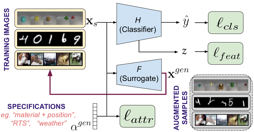
Figure 1: Overview of the problem setup and our attribute-guided adversarial training method.

We begin by defining the classifier parameterized by a set of neural network weights, $\theta$, as ${H}_{\theta}:\mathcal{X}_{s}\mapsto\mathcal{Y}$, where $\mathcal{X}_{s}$ denotes the space of the observed image data (or source) and $\mathcal{Y}$ denotes the label space for the task of interest.

Robustness to natural perturbations

Our goal is to train an $H_{\theta}$ that is robust to natural perturbations, which are typically larger in magnitude than the imperceptible $\ell_{p}$-bounded pixel-space perturbations, considered in the literature.

We consider a broad range of natural semantics-preserving perturbations that will not affect the predictions for the task under consideration – (a) Object-level shifts, where attributes of the object are manipulated so as to considerably change the appearance of the object, without changing the task label; such as changing the shape or size of an object in a color classification task. (b) Geometric transformations, where the test image may be scaled, rotated, and shifted in arbitrary ways; and (c) Common image corruptions, which may occur in the real world like fog, image compression artifacts, blurs, and other forms of noise.

Most of these perturbations do not naturally fall within small $\ell_{p}$-norm ball deviations ($|\mathbf{x}-\tilde{\mathbf{x}}|_{p}\leq\epsilon$), for which most existing robustness methods are designed, and are bound to fail when the classifier encounters such data in the wild. However, making $\epsilon$ arbitrarily large in robustness formulations does not work in practice, since the image quality degrades significantly. Hence, we propose a new framework to design models that are robust to such natural perturbations.

4 Attribute Guided Adversarial Training

Let us denote an image by $\mathbf{x}_{\alpha}$ parameterized by a set of attributes $\alpha$ related to image formation (lighting, viewing angle, position) as well as abstract semantic information (color, shape, size, etc.). Manipulating images with new combinations of attributes that are not seen in the training set, requires access to the underlying physical generative processes, which is unrealistic. We do not assume direct access to such deterministic mechanisms.

Our goal is to train classifiers robust to natural perturbations along attributes in $\alpha$ that are specified a priori. Inspired by recent developments in robust optimization and adversarial training (Madry et al. 2018), we consider the following worst-case problem around $N$ attributes of the training data:

$$\min_{\theta\in\Theta}\sum_{i=1}^{N}\max_{|\hat{\alpha}_{i}-\alpha_{i}|\leq\epsilon}\ell(\theta;(\mathbf{x}_{\hat{\alpha}_{i}},y_{i})),$$ (1)

where $\ell(\cdot)$ is the cross-entropy loss.

The solution to worst-case optimization in Equation 1 guarantees good performance against test data that is distance $\epsilon$ away from the training data in the attribute space. In other words, we expect the model learned using (1) to be robust against $\epsilon$-bounded natural perturbations. Interestingly, as we will empirically show later, models learnt using (1) perform better than existing pixel-level techniques even on $\ell_{p}$-bounded imperceptible perturbations.

Although the structure of the attribute-guided adversarial training problem may look similar to standard adversarial training, we explain next why solving Eq (1) is significantly more challenging and requires us to make several algorithmic innovations. Note that (1) solves a min-max optimization problem, with the inner maximization generating natural perturbations by maximizing the classification loss over attribute space, and the outer minimization finding model parameters by minimizing the loss on natural perturbations of the training data generated from the inner maximization. The success of this method crucially relies on solving the inner optimization problem. Motivated by the standard adversarial training, one might be temped to approximately solve the re-parameterized inner optimization problem

$$\underset{|{\delta}|_{p}\leq\epsilon}{\max}l(\theta;(\mathbf{x}_{{\alpha}_{i}+{\delta}},y_{i})),$$ (2)

and generate the natural perturbations $\mathbf{x}_{\hat{\alpha}_{i}}^{*}$ using projected gradient descent (PGD) as:

$${\delta_{i}}^{*}:=\mathcal{P}_{\epsilon}(\delta_{i}-\lambda\nabla_{\delta}l(\theta;(\mathbf{x}_{{\alpha}_{i}+{\delta}},y_{i}))),$$ (3)

where $\lambda$ is the gradient step and $\mathcal{P}_{\epsilon}$ is projection on $l_{p}$ ball of radius $\epsilon$. However, there are two fundamental issues with this approach making it infeasible in practice: first, we cannot compute gradients as we do not have access to the attribute space; and second, we do not have access to the true generative mechanism conditioned on the attributes.

4.1 Proposed Approach

Surrogate Functions

We propose to use differentiable surrogate functions parameterized by attributes to overcome the limitation described above. In other words, we have $\mathbf{x}_{\alpha+\delta}\approx F_{\delta}(\mathbf{x}_{\alpha})$, where $F_{\delta}$ is differentiable. Typically, exact perturbations $\mathbf{x}_{\alpha+\delta}=F_{\delta}(\mathbf{x}_{\alpha})$ can be performed for PGD attacks or other $\ell_{p}$ norm bounded attacks. However, in our case accessing the true generative process to manipulate images along $\alpha$ is not feasible. For example, we cannot rely on deterministic functions to manipulate semantic features in the image like size, shape or texture of an object. As a result, we resort to using approximate image manipulators in the form of surrogate functions which act as proxies to the true generative process. Depending on the type of attributes against which we wish to train for robustness, the surrogate function can take different forms:

• generative editing models for semantic perturbation that is learned from the training data itself,

• analytical functions for geometric transformations in the form of spatial transformers (STNs), or

• an analytical approximation (or tractable upper bound) of the natural perturbation space.

For example, if we want a classifier robust to unknown affine transforms then $F$ is the spatial transformer layer parameterized by $\alpha$ which now represents $6$ parameters controlling rotation, scale, and shift of the image.

Note that we do not assume access to any additional data other than the clean training dataset $\mathcal{X}_{s}$, and specification of the class of functions against which robustness is desired. While such surrogate functions only approximate the natural perturbations, we show that they are sufficient for enabling us to make classifiers more robust to natural perturbations.

Iterative Training Procedure

Having access to attribute parameterized surrogate function, we aim to solve (1). Note, the success of the adversarial training is dependent on the quality of the generated perturbations. Thus, we aim to generate natural perturbations that have a larger coverage over the specified attribute space than the training samples images $\mathbf{x}_{s}$. Consider the classifier $H_{\theta}$ which outputs the predicted class $\hat{y}$ and intermediate features $z$, let the surrogate function ${F}$ be parameterized by the attribute vector $\alpha$. We propose an iterative training procedure called Attribute-Guided Adversarial Training (AGAT) detailed in Algorithm 1. Our algorithm has two objectives: to minimize the classification loss over input images and to maximize the divergence between the training samples and generated perturbations. Thus, the key idea here is to explore novel and hard images that only vary along the specified attributes. To achieve this, we impose a constraint that maximizes the distance between features of dataset images and perturbed images. Additionally, since we would also like to explore new regions in the attribute space, we impose a similar constraint on the attributes of perturbed images.

We express this constraint as the loss function given by:

$$\begin{split}\ell_{const}=\lambda_{1}\ell_{feat}+\lambda_{2}\ell_{attr},~{}~{}\lambda_{1},\lambda_{2}\in(0,1)\\ \text{where~{}~{} }\ell_{feat}=||\mathbf{z}-\mathbf{z^{gen}}||_{2}^{2},\text{~{}and~{}~{}}\ell_{attr}=||\alpha-\alpha^{gen}||_{2}^{2}\end{split}$$ (4)

To ensure that the generated images belong to the same class as the input image, we combine classification loss with respect to the ground truth label $\mathbf{y}$ with consistency regularization with respect to the predicted label $\mathbf{\hat{y}}$ of $\mathbf{x}$.

$$\ell_{cls}=\ell_{BCE}(\mathbf{y},\mathbf{y^{gen}})+\ell_{BCE}(\mathbf{\hat{y}},\mathbf{y^{gen}})$$ (5)

The overall loss function is computed as the Lagrangian:

$$\ell_{AGAT}=\ell_{cls}-\beta\cdot\ell_{const}$$ (6)

Intuitively, $\ell_{cls}$ encourages the augmented images to belong to the same class-label as the input image, while the constraint $\ell_{const}$ encourages the adversarial learning algorithm to perturb the image features as well as the attributes away from the input features and attributes.

Algorithm 1 Attribute-Guided Adversarial Training

  Input: Source dataset $\mathcal{D}_{S}=\{\mathbf{x}_{t},y_{t}\}_{i=t}^{T}$

  Output: learned weights $\theta$

1:  Initialize: $\theta\leftarrow\theta_{0}$, $\mathcal{D}^{aug}_{S}\leftarrow\mathcal{D}_{S}$

2:  for $n=1\dots N_{epochs}$ do

3:     if $n<N_{pre}$ then

4:        for $t=1:T$ do

5:           $\theta\leftarrow\theta-\eta\triangledown\ell_{cls}(\theta;(\mathbf{x}_{t},y_{t}))$

6:     else

7:        if $n~{}\text{mod }N_{aug}=0$ then

8:           for $t=1\ldots T_{aug}$ do

9:              sample ${(\mathbf{x}_{t},y_{t})}_{t=1}^{T_{aug}}$ from $\mathcal{D}_{S}$

10:              $z_{t},\hat{y}_{t}=H(\mathbf{x_{t}})$

11:              Initialize: $\alpha_{t}^{gen}$

12:              for $i=1\ldots M$ do

13:                 $z^{gen}_{t},\hat{y}^{gen}_{t}=H(\mathbf{x}_{t},\alpha_{t}^{gen})$

14:                 $\mathbf{x}_{t}^{gen}\leftarrow f(\mathbf{x}_{t},\alpha_{t}^{gen})$

15:                 $\alpha_{t}^{gen}\leftarrow\alpha_{t}^{gen}-\mu\triangledown(\cdot\ell_{cls}-\beta\cdot\ell_{cons})$

16:              $\mathcal{D}_{S}^{aug}\leftarrow\mathcal{D}_{S}^{aug}\cup\mathbf{x}_{t}^{gen}$

17:        else

18:           for $(\mathbf{x}_{t},y_{t})\in\mathcal{D}^{aug}_{S}$ do

19:              $\theta\leftarrow\theta-\eta\triangledown\ell(\theta;(\mathbf{x}_{t},y_{t}))$

We first pre-train the classifier only on the source samples $\mathbf{x}_{s}$ for $N_{pre}$ epochs. Then, we initiate our augmentation process. To generate new samples, we minimize Equation 6 and update the attribute vector for $M$ update steps as:

$$\alpha^{gen}\leftarrow\alpha^{gen}-\mu\triangledown\ell_{AGAT}.$$ (7)

Finally, synthetic images are generated using the surrogate function $\mathbf{x}^{gen}\leftarrow F(\mathbf{x},\alpha^{gen})$, and appended to the training data. This adversarial data augmentation is performed after every $N_{aug}$ epochs during which $T_{aug}$ images are generated. The total number of augmented samples is expressed as a percentage of the number of training samples so as to allow fair comparison across datasets and types of perturbations. The pseudocode for AGAT is shown in Algorithm 1.

The distinguishing factor for AGAT is that we perturb the attribute space and use surrogate functions to synthesize images, while previous adversarial augmentation protocols such as M-ADA (Qiao, Zhao, and Peng 2020) and GUD (Volpi et al. 2018) perturb only in the pixel-space, thus being restricted to $\ell_{p}$ perturbations. It is important to note that our method is agnostic to the choice of surrogate functions, which can take the form of additive noise, affine transformation in pixel-space, or conditional generative adversarial networks (Mirza and Osindero 2014) trained to transform an input image according to an input attribute vector.

5 Experiments

In this section, we introduce the three types of robustness specifications that we experiment with, along with details about the datasets, baselines, and metrics used for each.

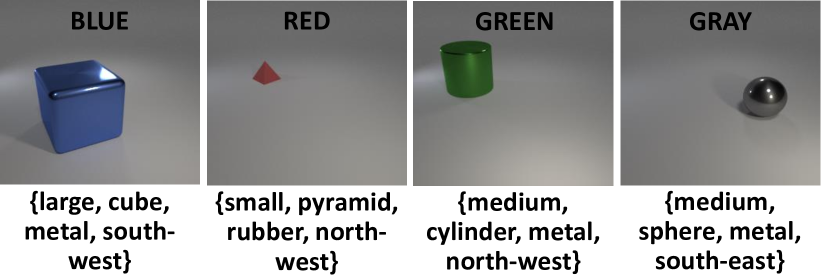
Figure 2: Examples of images from CLEVR-Singles and the color labels and (size, shape, material, position) attributes.

Attribute	Train	Test
Size and Position	(small, NW), (medium, NE), (large, SE)	(small, SE), (medium, NW), (large, SW)
Material and Position	(metal, NW), (rubber, NW), (metal, NE), (rubber, NE)	(rubber, SW), (metal, SW), (rubber, SE), (metal, SE)

Table 1: The train and test splits for our experiments with semantic object-level perturbations for CLEVR-Singles.

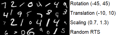
Figure 3: RTS-perturbed MNIST images.

5.1 Semantic Object-Level Perturbations

One class of real-world perturbations is when properties or attributes of images or objects in images change at test time. These changes do not affect the classification label, but significantly change the appearance of the image. For instance, consider the task of color classification in objects of varied shapes and textures. Here, red metallic spheres and red rubber cubes both belong to the class label “red”, however may appear very different in their shapes and textures. Thus, if only red metallic cubes are seen during training, conventional classifier predictions for test images consisting of red rubber cubes can fail to generalize. Thus, although the class label is invariant to such semantic factors, robustness to perturbations along these factors is desirable.

Dataset:

To study the problem of such object-level shifts along semantic factors of an image in a controlled fashion, we create a new benchmark called CLEVR-Singles by modifying the data generation process from CLEVR (Johnson et al. 2017). We create images of single objects having one of eight colors, and use color classification as our task in this paper. Each object has four variable attributes that do not affect the color class of the image; these are: shape (cube, sphere, pyramid, or cylinder), size (small, medium, or large), material (rubber or metal), and position (northwest, southwest, northeast, southeast). While the objects are generated at continuous $(X,Y,Z)$ world coordinates, we assign them a discrete position class for our experiments. Object-level perturbations can be made over these four attributes for our robustness experiments. In other words, it is known that one or more of {shape, size, material, position} of the image may change at test-time without knowing the magnitude or combinations of the change. We split the dataset based on a combination of attributes as shown in Table 1; for instance only certain combinations of size and position are observed in the training set, but robustness is expected from the color classifier on unknown combinations.

AttGAN as the Surrogate Function:

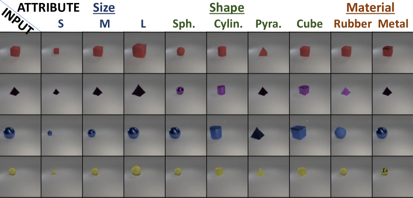
Figure 4: Images generated by AttGAN for the images in column 1, conditioned on attributes.

Conditional generative adversarial networks (cGANs) have been shown to perform exceptionally well on image-to-image translation in various domains (Isola et al. 2017; Zhang et al. 2017; Karras, Laine, and Aila 2019). AttGAN (He et al. 2019) is one such conditional GAN which is trained to manipulate attributes of input face images. Thus given an image and a vector of desired attributes, AttGAN can manipulate the face image along the desired attribute dimensions. We leverage this powerful image manipulation technique as our surrogate function $\mathbf{x}^{gen}=F_{GAN}(\mathbf{x},\alpha)$. Formally, we define the attribute vector to be a 13-dimensional binary hash-code with 1 and 0 indicating presence or absence of an attribute. For each experiment, we train the AttGAN on the training dataset outlined in Table 1 to generate 128x128 images, with a learning rate of $2\mathrm{e-}4$ for 100 epochs on a single 16GB GPU. Examples of images generated by AttGAN are shown in Figure 4, when manipulating certain attributes such as size, shape, and material of the object.

Baselines:

For the color classification task on CLEVR-Singles images, we compare against two pixel-level domain augmentation baselines: GUD (Volpi et al. 2018) which performs adversarial data augmentation to generate fictitious target domains, and M-ADA (Qiao, Zhao, and Peng 2020) which uses a meta-learning framework to generate multiple domains of samples. We also report the performance of a classifier directly without any adversarial training as a naive baseline. The same classifier architecture is used for each baseline for fair comparison. All models are trained for $15$ epochs including pre-training epochs $N_{pre}=5$, batch-size $64$, and $M=15$ update steps for adversarial augmentation. The number of augmented samples $T_{aug}$ is $30\%$ of the original source data, and augmentation interval $N_{aug}$ is fixed at 2 epochs. For our model the coefficients in Equations 4, and 5 are: $\lambda_{1}=0.5,\lambda_{2}=0.5,\beta=0.25$. The learning rates $\eta,\mu$ for the classifier and adversarial augmentation are both 5e-5.

Results:

Method	Source	Size+Pos.	Mat.+Pos.
B	99.81	89.92	59.90
GUD (2018)	99.94	93.69	65.03
M-ADA (2020)	99.96	94.52	65.50
Ours	99.97	95.22	69.49

Table 2: Classification accuracy for color-classification on CLEVR-Singles. Source and target sets are split on size+position attribute for the third column, and Material+Position for the fourth column.

The test classification accuracies for different splits are reported in Table 2. We observe that our model is better than all baselines considered here, with a boost of $5$ percentage points in accuracy on the harder experiment along Material+Position.

Analysis:

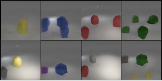
Figure 5: Visualization of the effect of weight $\beta$ of the constraint loss $\ell_{const}$ on the generated images. Row 2 has higher $\beta$ than Row 1. Illustration also shows that AttGAN is able to generate multiple objects (of same color for Row 1 and different colors for Row 2), though absent in training data.

In Figure 5, we show 8 different examples generated by AttGAN during adversarial training. We can see the effect of the coefficient $\beta$, from the constraint loss $\ell_{const}$ in eq (6), in exploring the attribute space. An appropriately chosen value for $\beta$ encourages useful perturbations without violating the class-label consistency cost $\ell_{cls}$ as seen in the top row of Figure 5. On the other hand, a higher $\beta$ would mean a higher weight for exploring the regions (or combinations) in attribute space not seen in training. In the bottom row we see that a high $\beta$ encourages novel attribute exploration at the cost of higher classification error as a result of generating objects with different colors within the same image. It is noteworthy that AttGAN is able to generate images with multiple objects, even when it trained on images with only a single object, thus demonstrating its suitability to explore novel attributes using the proposed AGAT training.

5.2 Geometric Transformations

Another common class of perturbations is geometric transformations, i.e. a composition of rotation, translation, and scaling of an image. These perturbations are common since cameras may capture a scene from different orientations, distances, and inclinations. It is well known that standard image classifiers are not robust to these common perturbations (Cohen and Welling 2014).

Dataset:

We address this problem in the digit classification setting, with the training images from MNIST (LeCun et al. 1998), and the test images that are perturbed along rotation-translation-scale (RTS), as shown in Figure 3. We use the standard RTS setup (Jaderberg et al. 2015) with angle of rotation in $(-45,45)^{\circ}$, translation in $(-10,10)$ pixels in both directions, and a scale factor in the range $(0.7,1.3)$.

Surrogate Function:

The attributes of interest, $\alpha$, consist of a $2\times 3$ affine matrix that controls rotation, translation, and scale. To perform affine transformations on the image with a perturbed $\alpha$, we use Spatial Transformer Networks (STN) (2015) which allow differentiable spatial manipulation of input images in a convolutional neural network, such as RTS and or general warping. The perturbed images are generated as: $\mathbf{x}^{gen}=F_{STN}(\mathbf{x}_{s},\alpha)$.

Baselines:

We compare the robustness performance to RTS perturbations with a naive baseline, denoted by (B), that is only trained on the standard MNIST dataset, and pixel-level perturbation methods MADA (Qiao, Zhao, and Peng 2020) and GUD (Volpi et al. 2018). Additionally, we also use the RTS perturbation sets generated by (Wong and Kolter 2020) (PS) and use them as augmented training samples. All models are trained for 12 epochs including pre-training epochs $N_{pre}=5$, with a batch-size $64$, and $M=10$ update steps for adversarial augmentation. The number of augmented samples $T_{aug}$ is $30\%$ of the original source data, and augmentation interval $N_{aug}$ is fixed at 10 epochs. Our model the coefficients in Equations 4, and 5 are: $\lambda_{1}=1,\lambda_{2}=1,\beta=5$. The learning rate $\eta$ for the classifier is $1\mathrm{e-}4$ and $\mu$ for the adversarial augmentation is $0.1$.

Results:

Method	R	T	S	RTS
B	84.44	27.67	95.76	21.91
GUD (2018)	86.08	29.09	97.89	23.10
MADA (2020)	87.37	29.25	98.32	22.68
PS (2020)	87.86	45.36	96.00	39.38
Ours ($T_{aug}\text{=}30\%$)	84.93	52.95	96.11	41.43

Table 3: Results on the MNIST-RTS robustness benchmark for rotation (R), translation (T), scaling (S), and random combination (RTS).

We report digit classification accuracies on the target test set containing only rotations (R), only translations (T), only skew (S), as well as a random combination of RTS. Our model performs well on all four metrics, and beats the perturbation sets (PS) even though their augmentation model has access to RTS perturbations during training. In particular, we observe a significant improvement compared with MADA and GUD, in the robustness on the translation experiment, which is the hardest task among the three.

Analysis

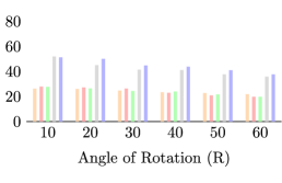
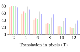
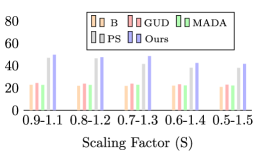
Figure 6: Comparison of random RTS accuracies when controlling each parameter to a max. value. Left: R, Center: T, Right: S

$\mathbf{N_{aug}}$	$\mathbf{T_{aug}}$	R	T	S	RTS
1	10	84.12	43.33	96.65	34.12
	30	83.80	54.17	95.89	40.46
	50	84.49	59.97	96.29	47.62
	70	84.35	62.76	96.24	51.13
2	10	84.97	47.21	96.41	36.84
	30	84.93	52.95	96.11	41.43
	50	86.35	61.07	95.76	47.59
	70	84.59	62.75	95.79	50.28

Table 4: The effect of augmentation interval ($N_{aug}$) at different percentages of augmented samples ($T_{aug}$).

Loss	$\mathbf{T_{aug}}$	R	T	S	RTS
GT	10	85.41	29.48	96.74	23.57
	30	84.82	48.46	96.75	37.80
	50	84.17	52.44	95.86	41.82
	70	84.07	55.14	95.70	44.20
GT + CR	10	84.97	47.21	96.41	36.84
	30	84.93	52.95	96.11	41.43
	50	86.35	61.07	95.76	47.59
	70	84.59	62.75	95.79	50.28

Table 5: The effect of classification loss function at different percentages of augmented samples. GT denotes the first term and CR is consistency regularization in Eq (5).

The pixel-level perturbation methods still perform reasonably well on rotation and scale experiments in Table 3 because in each case the rotations/translations/scale are randomly sampled, resulting in several test examples that are very close to the training examples (with no RTS). In order to resolve this further, we study the performance by controlling the magnitude of R, T, and S in the test set. Figure 3 shows the bar-plots when the range of rotation is varied from $(-10,10)$ to $(-60,60)$, translation from $(-2,2)$ to $(-12,12)$ pixels, and scaling factor from $(0.9,1.1)$ to $(0.5,1.5)$. It can be observed that at higher severity of perturbation, our model (in blue) significantly outperforms all baselines. The model trained with Perturbations Sets (2020) (in gray) is competitive at lower severities.

We also analyze the effect of the number of augmented samples ($T_{aug}$) expressed as a percentage of the size of the training data, while controlling for the augmentation interval $N_{aug}$. As expected, larger number of augmented samples improve robustness even higher than in table 3 (which fixes number of additional augmented examples at $30\%$ for all baselines). Larger augmentation intervals contribute positively at lower percentages of augmented samples.

Finally, we perform an ablation study with and without the consistency regularization defined in Eq (5) and show that the regularization indeed helps improve performance.

5.3 Common Image Corruptions

Image corruptions are another common class of perturbations. These can occur due to image digitization artifacts, weather, camera calibration, and other sources of noise.

Dataset

The CIFAR10 dataset (Krizhevsky 2009) contains $50k$ training images belonging to $10$ classes. Recently, CIFAR10-C (Hendrycks and Dietterich 2018) which contains image corruptions for CIFAR10 images, was proposed to benchmark robustness of image classifiers, with 4 major and 15 fine-grained categories of corruption: Weather (fog, snow, frost), Blur (zoom, defocus, glass, motion), Noise (shot, impulse, Gaussian), and Digital (JPEG, pixelation, elastic transform, brightness, contrast). There are five levels of severity of corruptions; we focus on the highest severity.

Surrogate Function:

We use a general surrogate function – a composition of additive Gaussian noise and Gaussian blur filter parameterized by $\mathbf{\alpha}=\{\alpha_{1},\alpha_{2}\}$:

$$\mathbf{x}^{gen}=\frac{1}{\sqrt{2\pi\alpha_{1}^{2}}}e^{-\frac{\mathbf{x}^{2}}{2\alpha_{1}^{2}}}+n\text{, ~{}where~{} }n\sim\mathcal{N}(0,\mathbf{\alpha}_{2}).$$ (8)

We evaluate the performance gains using this surrogate function with the proposed AGAT training on the challenging CIFAR-10-C dataset.

Baselines:

Test-Time Training (TTT) (Sun et al. 2020) is a recent approach in which a classifier is trained only on source data, but the test sample is utilized to update the classifier during inference. Adversarial Logit Pairing (ALP) (Kannan, Kurakin, and Goodfellow 2018), a technique for defending against adversarial attacks, and pixel-wise domain augmentation techniques MADA (Qiao, Zhao, and Peng 2020) and GUD (Volpi et al. 2018) are also considered as baselines. We use ResNet-26 (He et al. 2016) specially designed for CIFAR-10 (2015), with group normalization (Wu and He 2018) which is stable with different batch sizes. This acts as the naive classifier-only baseline (B). We also consider the classifier trained with an auxiliary self-supervised task of angle prediction (Gidaris, Singh, and Komodakis 2018) (B+SS). Our joint-training (JT) baseline is from TTT based on (Hendrycks and Dietterich 2018).

We compare three versions of our model: with additive noise only, with Gaussian filtering, and with a composition of Gaussian filter and noise. Our models are trained for 150 epochs including pre-training epochs $N_{pre}\mathrm{=}100$, batch-size 128, and $M\mathrm{=}15$ update steps for adversarial augmentation. The number of augmented samples is $30\%$ of the original source data, and augmentation interval $N_{aug}$ is fixed at 2 epochs. For our model the coefficients in Equations 4, and 5 are: $\lambda_{1}=0.5,\lambda_{2}=0.5,\beta=0.25$. The learning rates $\eta,\mu$ for the classifier and adversarial augmentation are both 5e-5.

Results

Method	Src.	W	B	N	D	Avg.
B	90.6	70.6	69.0	45.5	71.6	66.4
B+SS	91.1	70.6	68.5	48.7	69.7	67.0
GUD	-	71.7	59.2	30.5	64.7	58.3
MADA	-	75.6	63.8	54.2	65.1	65.6
JT	91.9	71.7	69.0	50.6	71.6	68.3
ALP	83.5	60.9	74.7	75.4	68.5	70.0
TTT	92.1	73.7	71.3	54.2	73.4	70.5
Ours (b. only)	91.3	78.4	75.1	49.3	75.4	70.0
Ours (n. only)	90.3	75.0	73.3	62.4	73.1	71.3
Ours	89.3	77.8	74.1	65.8	71.6	72.3

Table 6: Comparison of classification accuracies on CIFAR-10-C corruption categories (Weather, Blur, Noise, Digital). Our best scores are underlined; overall best are bold.

In Table 6 we show the classification accuracies on CIFAR10-C. It can be seen that our method consistently outperforms all baselines overall, and also on three of the four categories of corruptions (weather, blur, and digital). It is interesting to note that the ALP performance on the Noise category is distinctly greater than all previous methods, potentially because it is designed to defend against projected gradient descent adversarial attacks (Madry et al. 2017). ALP uses a similar loss function as Equation 5 to train the classifier, but still operates in pixel-space and does not perturb the attribute space. In Table 6 we also demonstrate that our models which uses only blur or only noise as surrogate are also better than previous state-of-the art. Note that the “noise only” model is in essence a pixel-level perturbation achieved by only perturbing along the variance parameter using AGAT training, and yet we see a significant boost in performance over all other pixel-level additive noise methods. Similarly, the “blur only” model also gives performance boosts on weather and digital categories, further indicating the general applicability of our AGAT training approach.

6 Conclusion

In this paper, we propose a new adversarial training strategy for robustness against large perturbations that are common in practical settings. Our adversarial training algorithm perturbs the attribute space to synthesize new images instead of pixel-level perturbations which are common to the robustness literature. The new CLEVR-Singles dataset that we have created can be used in future work for studying robustness to semantic shifts. We extensively evaluate AGAT training on three benchmarks and achieve state-of-the-art performance. We empirically show that AGAT is applicable to a three types of naturally occurring perturbations, and can be used with different classes of surrogate functions. AGAT can potentially be applied to a broad range of robustness problems not limited to classification.

Broader Impact

The concept of robustness is critical when it comes to deploying machine learning systems in practical settings where input signals may undergo perturbations due to weather (such as fog, smog, rain), digital corruptions in transmission, or changes in camera inclinations causing geometric transformations or artifacts such as defocusing, or motion blur. Our method for developing robust classifiers is broadly applicable if such classes of perturbations are known a priori.

Robustness research is also crucial for avoiding or removing unintended biases that may percolate from the training data into the classification model. Recent studies (Bolukbasi et al. 2016; Zhao et al. 2017; Hendricks et al. 2018) have shown that models trained on biased data can in fact amplify this bias when performing inference on test samples. We believe that work in the lines of AGAT could be potentially used for mitigating social biases due to biased training data, such as gender or racial biases.

Appendix

This appendix contains further details about the creation of the CLEVR-Singles dataset, additional sample images generated by AGAT, model details, and fine-grained results on the CIFAR-10-C benchmark.

Appendix A CLEVR-Singles Dataset Creation

The CLEVR-Singles dataset has been created to allow a diagnostic setup with discrete and controllable set of attributes for our robustness experiments for semantic object-level perturbations. In this section we delineate the dataset creation process and provide more examples from the dataset.

We use Blender (Blender Online Community 2018) to render images in CLEVR-Singles. Every scene contains a single object, have a randomly chosen size, shape, material, position, and color. Our code for rendering these images is a modification of the data creation process for the CLEVR dataset (Johnson et al. 2017). The choices for each property of the object are shown in Table 7.

Property	Choices
Color	gray, red, blue, green, brown, purple, cyan, yellow
Size	large (1.2), medium (0.9), small (0.6)
Shape	Cube, Sphere, Cylinder, Pyramid
Material	Rubber, Metal
Position	NW, NE, SW, SE
Rotation	$\theta\in[-180,180]$

Table 7: List of properties that can be assigned to an object to render the images in CLEVR-Singles.

Size refers to the height or diameter of the shapes which are symmetric along $x$ and $y$ axes. In terms of 3D coordinates, the objects are placed at the position $(X,Y,Z)$ such that:

$$X\in[-3,3],Y\in[-3,3],Z=0.5*size.$$

For our experiments, we define position to be one of the four quadrants of the $xy$ plane and denote these by NW, NE, SW, SE, which allows us to easily split the dataset for robustness experiments.

The positions of the lighting and camera and are slightly jittered to introduce variation. The objects are rotated at a random angle while placing. We generate images of size $256\times 256$ using a tile size of $128$ for rendering. The CLEVR-Singles dataset contains $50000$ images for training, $10000$ for validation, and $10000$ test samples. Each image takes approximately 5 seconds to render using a single GPU, and can also be rendered on CPU at 8 seconds per image. Along with the images, scene graphs are also generated which contain labels for each attribute, color, and other properties.

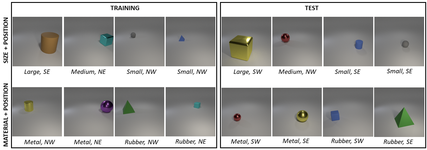
Figure 7: Sample images from the training and test splits for robustness experiments on the CLEVR-Singles dataset. The first row shows the train-test split on the attributes size+position, and the second row for material+position.

For our experimental setup for robustness experiments, we split the dataset into training and test splits according to specific attributes in Table 8.

Attribute	Train	Test
Size and Position	(small, NW), (medium, NE), (large, SE)	(small, SE), (medium, NW), (large, SW)
Material and Position	(metal, NW), (rubber, NW), (metal, NE), (rubber, NE)	(rubber, SW), (metal, SW), (rubber, SE), (metal, SE)

Table 8: The train and test splits for our experiments with semantic object-level perturbations for CLEVR-Singles.

Illustrative examples are shown in Figure 7 with the first row showing samples from training and test splits for size+position, and the second row for material+position. The data-generation code and train-test splits for robustness experiments will be made publicly available upon publication.

Appendix B AGAT-Generated Images

We provide additional samples generated by attribute-guided adversarial training algorithm (AGAT) for each of our experiments.

Semantic Object-Level Perturbations:

Figure 9 shows the images generated by AttGAN (He et al. 2019) during AGAT. It can be seen that AttGAN is able to explore various sizes, materials during the augmentation, as well generate novel scenes with multiple objects which are not present in the training dataset.

Geometric Transformations:

Figure 8 shows the images generated by STN (Jaderberg et al. 2015) during AGAT training. It can be seen that rotations, translations, skew, and combinations of these are generated.

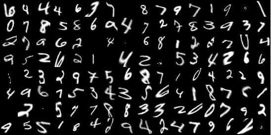
Figure 8: Examples of images generated by AGAT for MNIST. AGAT is able to explore the attribute space and generate images with different rotation, translations, and skews.

Common Image Corruptions:

Figure 10 shows the images during AGAT training on the CIFAR-10 dataset using additive Gaussian noise and blur as the surrogate function.

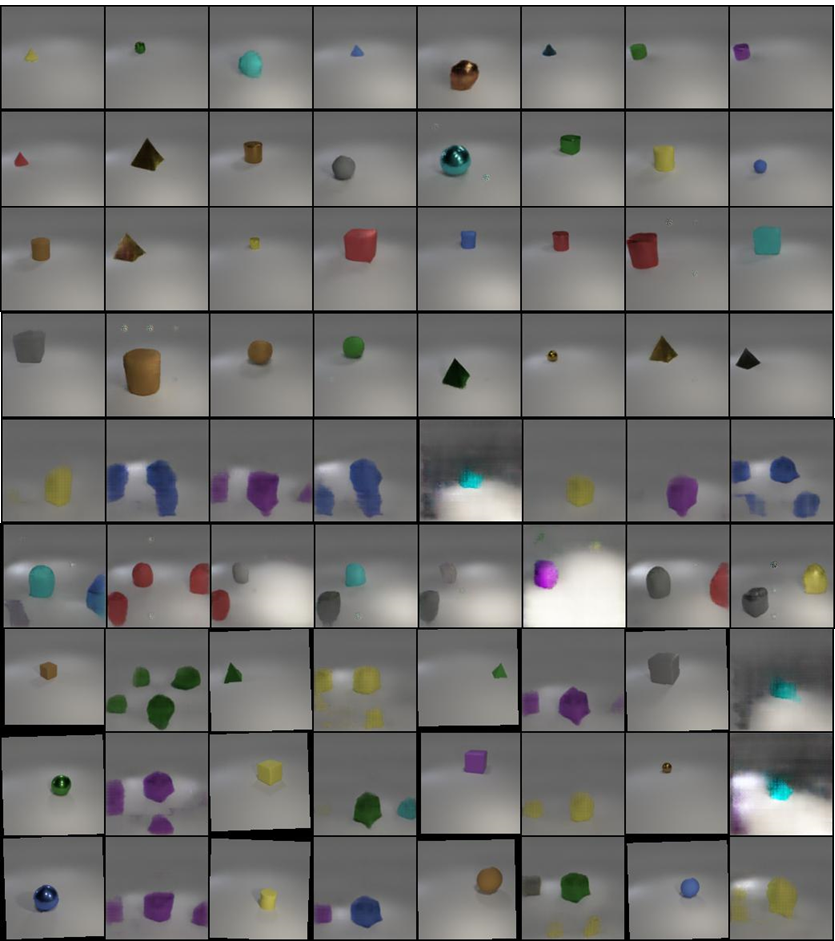
Figure 9: Examples of images generated by AGAT for the CLEVR-Singles dataset. The AttGAN generator is able to explore the attribute space and generate images with different attributes, as well as novel scenes such as those containing multiple objects.

Method	SRC	Fog	Snow	Frst	Zoom	Defo	Glas	Motn	Shot	Impl	Gaus	JPEG	Pixl	Elas	Brit	Cont	Avg $\pm$ Std
B	90.6	73.1	74.5	63.3	73.6	74.9	49.8	77.6	49.1	42.6	44.9	71.3	54.9	73.4	87.2	71.2	66.4 $\pm$ 13.2
B+SS	91.1	71.9	74.4	65.6	73.7	76.3	48.3	75.7	52.8	43.9	49.5	70.2	44.2	72.6	86.5	75.0	67.0 $\pm$ 13.3
GUD	-	68.3	76.8	70.0	62.9	56.4	53.5	63.9	36.9	22.3	32.4	74.2	53.3	74.6	89.9	31.6	58.3 $\pm$ 18.9
MADA	-	69.4	80.6	76.7	68.0	61.2	61.6	64.2	60.6	45.2	56.9	77.1	52.3	75.6	90.8	29.7	65.6 $\pm$ 14.7
JT	91.9	72.5	75	67.5	73.6	75.8	51.5	75.2	54.7	46.6	50.6	71.3	48.4	76	87.4	74.7	68.3 $\pm$ 12.3
ALP	83.5	35.2	74.8	72.8	76.9	75	74.4	72.6	77.1	71.7	77.3	81.1	79.8	77.0	78.3	26.4	70.0 $\pm$ 15.7
TTT	92.1	74.9	76.1	70.0	76.1	78.2	53.9	77.0	58.2	50.0	54.4	72.8	52.8	77.4	87.8	76.1	70.5 $\pm$ 11.4
Ours (blur only)	91.3	77.0	76.5	71.2	79.7	83.8	57.9	79.0	51.5	49.1	47.4	70.5	52.9	75.0	87.0	78.7	70.6 $\pm$ 13.1
Ours (noise only)	90.3	76.1	75.6	73.3	77.2	80.3	57.6	78.0	64.9	56.3	65.9	73.4	57.2	72.8	85.8	76.3	71.3 $\pm$ 8.7
Ours (both)	89.3	79.0	76.2	79.2	76.4	80.3	61.4	78.2	70.3	59.5	67.7	69.5	48.6	72.8	85.4	81.5	72.3$\pm$ 9.5

Table 9: Comparison of classification accuracies on CIFAR-10-C for each type of corruption. Underlined are our best scores, and bold are the overall best.

Appendix C Model Architectures

We use the same classifier for baselines as well as our model for fair comparison. For experiments on CLEVR-Singles, we use a color-classification neueral network with 4 convolutional layers with stride $2$ and kernel-size $3$, followed by 2 fully-connected layers. For experiments on MNIST, we use a classifier with two convolutional layers with kernel-size $5$ and stride $1$ and 3 fully-connected layers. For CIFAR-10-C experiments we use the classifier architecture used by (Sun et al. 2020) for fair comparison. The classifier is a ResNet (He et al. 2016) constructed specially for CIFAR-10 images and has 26 layers, group norm (Wu and He 2018) with 8 layers.

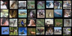
Figure 10: Examples of images generated by AGAT for the CIFAR-10 dataset. AGAT is able to explore the attribute space and generate images having varying degrees of noise and blur, which helps improve robustness on all 15 categories of corruptions as seen in Table 9.

Appendix D Additional CIFAR-10-C Results

In Table 9 we provide detailed comparison of our models with the baselines on the CIFAR-10-C benchmark for each of the 15 categories of corruptions. Our method shows consistent improvements across all 15 categories when compares with the classifier-only baselines (“B” and “B+SS”) as well as the current state-of-the-art model Test-Time Training (TTT) (Sun et al. 2020). M-ADA (Qiao, Zhao, and Peng 2020) is the best performing for “Snow” and “Brightness” images, but does not show consistent improvements on other categories. Similarly, ALP (Kannan, Kurakin, and Goodfellow 2018) is the best on all four noise categories, but suffers significantly on “Fog” ($35.2\%$) and “Contrast” ($26.4\%$) compared to all other baselines. Table 9 also shows the variances of each approach. Our approach (models using noise only, or both noise and blur) have a standard deviation lower than all other approaches.

References

- Blender Online Community (2018) Blender Online Community, A. 2018. Blender - a 3D modelling and rendering package. Blender Foundation, Stichting Blender Foundation, Amsterdam. URL http://www.blender.org.
- Bolukbasi et al. (2016) Bolukbasi, T.; Chang, K.-W.; Zou, J. Y.; Saligrama, V.; and Kalai, A. T. 2016. Man is to computer programmer as woman is to homemaker? debiasing word embeddings. In Advances in neural information processing systems, 4349–4357.
- Bulusu et al. (2020) Bulusu, S.; Kailkhura, B.; Li, B.; Varshney, P. K.; and Song, D. 2020. Anomalous Example Detection in Deep Learning: A Survey. IEEE Access 8: 132330–132347.
- Cohen and Welling (2014) Cohen, T. S.; and Welling, M. 2014. Transformation properties of learned visual representations. arXiv preprint arXiv:1412.7659 .
- Gidaris, Singh, and Komodakis (2018) Gidaris, S.; Singh, P.; and Komodakis, N. 2018. Unsupervised Representation Learning by Predicting Image Rotations. In International Conference on Learning Representations.
- Goodfellow, Shlens, and Szegedy (2014) Goodfellow, I. J.; Shlens, J.; and Szegedy, C. 2014. Explaining and harnessing adversarial examples. arXiv preprint arXiv:1412.6572 .
- He et al. (2016) He, K.; Zhang, X.; Ren, S.; and Sun, J. 2016. Deep residual learning for image recognition. In Proceedings of the IEEE conference on computer vision and pattern recognition, 770–778.
- He et al. (2019) He, Z.; Zuo, W.; Kan, M.; Shan, S.; and Chen, X. 2019. Attgan: Facial attribute editing by only changing what you want. IEEE Transactions on Image Processing 28(11): 5464–5478.
- Hendricks et al. (2018) Hendricks, L. A.; Burns, K.; Saenko, K.; Darrell, T.; and Rohrbach, A. 2018. Women also snowboard: Overcoming bias in captioning models. In European Conference on Computer Vision, 793–811. Springer.
- Hendrycks and Dietterich (2018) Hendrycks, D.; and Dietterich, T. 2018. Benchmarking Neural Network Robustness to Common Corruptions and Perturbations. In International Conference on Learning Representations.
- Isola et al. (2017) Isola, P.; Zhu, J.-Y.; Zhou, T.; and Efros, A. A. 2017. Image-to-image translation with conditional adversarial networks. In Proceedings of the IEEE conference on computer vision and pattern recognition, 1125–1134.
- Jaderberg et al. (2015) Jaderberg, M.; Simonyan, K.; Zisserman, A.; et al. 2015. Spatial transformer networks. In Advances in neural information processing systems, 2017–2025.
- Johnson et al. (2017) Johnson, J.; Hariharan, B.; van der Maaten, L.; Fei-Fei, L.; Lawrence Zitnick, C.; and Girshick, R. 2017. Clevr: A diagnostic dataset for compositional language and elementary visual reasoning. In Proceedings of the IEEE Conference on Computer Vision and Pattern Recognition, 2901–2910.
- Joshi et al. (2019) Joshi, A.; Mukherjee, A.; Sarkar, S.; and Hegde, C. 2019. Semantic adversarial attacks: Parametric transformations that fool deep classifiers. In Proceedings of the IEEE International Conference on Computer Vision, 4773–4783.
- Kannan, Kurakin, and Goodfellow (2018) Kannan, H.; Kurakin, A.; and Goodfellow, I. 2018. Adversarial logit pairing. arXiv preprint arXiv:1803.06373 .
- Karras, Laine, and Aila (2019) Karras, T.; Laine, S.; and Aila, T. 2019. A style-based generator architecture for generative adversarial networks. In Proceedings of the IEEE conference on computer vision and pattern recognition, 4401–4410.
- Krizhevsky (2009) Krizhevsky, A. 2009. Learning Multiple Layers of Features from Tiny Images. Master’s thesis, University of Toronto .
- LeCun et al. (1998) LeCun, Y.; Bottou, L.; Bengio, Y.; and Haffner, P. 1998. Gradient-based learning applied to document recognition. Proceedings of the IEEE 86(11): 2278–2324.
- Liu et al. (2018) Liu, H.-T. D.; Tao, M.; Li, C.-L.; Nowrouzezahrai, D.; and Jacobson, A. 2018. Beyond pixel norm-balls: Parametric adversaries using an analytically differentiable renderer. arXiv preprint arXiv:1808.02651 .
- Madry et al. (2017) Madry, A.; Makelov, A.; Schmidt, L.; Tsipras, D.; and Vladu, A. 2017. Towards deep learning models resistant to adversarial attacks. arXiv preprint arXiv:1706.06083 .
- Madry et al. (2018) Madry, A.; Makelov, A.; Schmidt, L.; Tsipras, D.; and Vladu, A. 2018. Towards Deep Learning Models Resistant to Adversarial Attacks. In International Conference on Learning Representations.
- Mirza and Osindero (2014) Mirza, M.; and Osindero, S. 2014. Conditional generative adversarial nets. arXiv preprint arXiv:1411.1784 .
- Qiao, Zhao, and Peng (2020) Qiao, F.; Zhao, L.; and Peng, X. 2020. Learning to learn single domain generalization. In Proceedings of the IEEE/CVF Conference on Computer Vision and Pattern Recognition, 12556–12565.
- Raghunathan, Steinhardt, and Liang (2018) Raghunathan, A.; Steinhardt, J.; and Liang, P. 2018. Certified Defenses against Adversarial Examples. In International Conference on Learning Representations.
- Recht et al. (2018) Recht, B.; Roelofs, R.; Schmidt, L.; and Shankar, V. 2018. Do cifar-10 classifiers generalize to cifar-10? arXiv preprint arXiv:1806.00451 .
- Russakovsky et al. (2015) Russakovsky, O.; Deng, J.; Su, H.; Krause, J.; Satheesh, S.; Ma, S.; Huang, Z.; Karpathy, A.; Khosla, A.; Bernstein, M.; et al. 2015. Imagenet large scale visual recognition challenge. International journal of computer vision 115(3).
- Sinha, Namkoong, and Duchi (2018) Sinha, A.; Namkoong, H.; and Duchi, J. 2018. Certifying Some Distributional Robustness with Principled Adversarial Training. In International Conference on Learning Representations.
- Sun et al. (2020) Sun, Y.; Wang, X.; Liu, Z.; Miller, J.; Efros, A. A.; and Hardt, M. 2020. Test-time training with self-supervision for generalization under distribution shifts. In International Conference on Machine Learning (ICML).
- Volpi et al. (2018) Volpi, R.; Namkoong, H.; Sener, O.; Duchi, J. C.; Murino, V.; and Savarese, S. 2018. Generalizing to unseen domains via adversarial data augmentation. In Advances in neural information processing systems, 5334–5344.
- Wong and Kolter (2020) Wong, E.; and Kolter, J. Z. 2020. Learning perturbation sets for robust machine learning. arXiv preprint arXiv:2007.08450 .
- Wu and He (2018) Wu, Y.; and He, K. 2018. Group normalization. In Proceedings of the European conference on computer vision (ECCV), 3–19.
- Xiao et al. (2020) Xiao, K.; Engstrom, L.; Ilyas, A.; and Madry, A. 2020. Noise or Signal: The Role of Image Backgrounds in Object Recognition. arXiv preprint arXiv:2006.09994 .
- Zhang et al. (2017) Zhang, H.; Xu, T.; Li, H.; Zhang, S.; Wang, X.; Huang, X.; and Metaxas, D. N. 2017. Stackgan: Text to photo-realistic image synthesis with stacked generative adversarial networks. In Proceedings of the IEEE international conference on computer vision, 5907–5915.
- Zhao et al. (2017) Zhao, J.; Wang, T.; Yatskar, M.; Ordonez, V.; and Chang, K.-W. 2017. Men Also Like Shopping: Reducing Gender Bias Amplification using Corpus-level Constraints. In Proceedings of the 2017 Conference on Empirical Methods in Natural Language Processing, 2979–2989.