Semi-Supervised Learning with Variational Bayesian Inference and Maximum Uncertainty Regularization

Abstract

We propose two generic methods for improving semi-supervised learning (SSL). The first integrates weight perturbation (WP) into existing “consistency regularization” (CR) based methods. We implement WP by leveraging variational Bayesian inference (VBI). The second method proposes a novel consistency loss called “maximum uncertainty regularization” (MUR). While most consistency losses act on perturbations in the vicinity of each data point, MUR actively searches for “virtual” points situated beyond this region that cause the most uncertain class predictions. This allows MUR to impose smoothness on a wider area in the input-output manifold. Our experiments show clear improvements in classification errors of various CR based methods when they are combined with VBI or MUR or both.

Introduction

Recent success in training deep neural networks is mainly attributed to the availability of large, labeled datasets. However, annotating large amounts of data is often expensive and time-consuming, and sometimes requires specialized expertise (e.g., healthcare). Under these circumstances, semi-supervised learning (SSL) has proven to be an effective means of mitigating the need for labels by leveraging unlabeled data to considerably improve performance. Among a wide range of approaches to SSL (van Engelen and Hoos 2019), “consistency regularization” (CR) based methods are currently state-of-the-art (Bachman, Alsharif, and Precup 2014; Sajjadi, Javanmardi, and Tasdizen 2016; Laine and Aila 2016; Tarvainen and Valpola 2017; Miyato et al. 2018; Verma et al. 2019; Xie et al. 2019; Berthelot et al. 2019b; Sohn et al. 2020). These methods encourage neighbor samples to share labels by enforcing consistent predictions for inputs under perturbations.

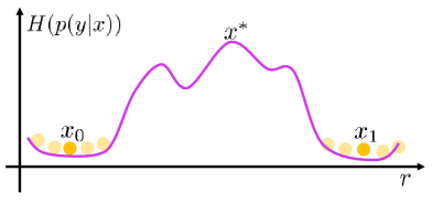
Figure 1: The most uncertain “virtual” point $x^{*}$ usually lies outside the vicinity of $x_{0}$ and is the most disruptive.

Although the perturbations can be created in either the input/feature space (data perturbation) or the weight space (weight perturbation), existing CR based methods focus exclusively on the former and leave the latter underexplored. Despite being related, weight perturbation (WP) is inherently different from data perturbation (DP) in the sense that WP directly reflects different views of the classifier $f$ on the original data distribution (e.g., $f_{w}(x)$ v.s. $f_{w^{\prime}}(x)$) while DP indirectly causes the classifier to adjust its view to adapt to different data distributions (e.g., $f_{w}(x)$ v.s. $f_{w}(x^{\prime})$). Therefore, we hypothesize that the two types of perturbations are complementary and could be combined to increase the classifier’s robustness. To implement WP, we treat the classifier’s weights $w$ as random variables and perform variational Bayesian inference (VBI) on $w$. This approach has several advantages. First, perturbations of $w$ can be generated easily via drawing samples from an explicit variational distribution $q_{\phi}(w|\mathcal{D})$. We also take advantage of the local reparameterization trick and variational dropout (VD) (Kingma, Salimans, and Welling 2015; Molchanov, Ashukha, and Vetrov 2017) to substantially reduce the sampling cost and variance of the gradients w.r.t. the weight samples, making VBI scalable for deep neural networks. Second, since VBI is a realization of the Minimum Description Length (MDL) framework (Hinton and von Cramp 1993; Honkela and Valpola 2004), a classifier trained under VBI, in principle, often generalize better than those trained in the standard way.

Standard DP methods (e.g., Gaussian noise, dropout) often generate perturbations in the vicinity of each data point and ignore those in the vacancy among data points, which means consistency losses equipped with standard DPs can only train locally smooth classifiers that do not generalize well in general. To overcome this limitation, we propose a novel consistency loss called “maximum uncertainty regularization” (MUR) of which the key component is finding for each real data point $x_{0}$ a neighbor “virtual” point $x^{*}$ that has the most uncertain class prediction given by the classifier $f$. During training, $f$ becomes increasingly confident about its predictions of the real data points and their neighborhood (otherwise, the training cannot converge). Thus, by choosing $x^{*}$ with the above properties, we can guarantee, with high probability, that i) $x^{*}$ is situated outside the vicinity of $x_{0}$, and ii) $x^{*}$ causes the biggest disruption to the classifier’s predictions (Fig. 1). This observation suggests that MUR enforces smoothness on a wider and rougher area in the input space than conventional consistency losses, hence, making the classifier generalize better. As MUR operates in the input space not the weight space, it is complementary to WP and in some cases, both can be used together.

In our experiments, we show that when strong data augmentation is not available, WP and MUR significantly boost the performance of existing CR based methods on various benchmark datasets.

Preliminaries

Consistency Regularization based Methods for Semi-supervised Learning

We briefly present two representative CR based methods namely $\Pi$-model (Laine and Aila 2016) and Mean Teacher (Tarvainen and Valpola 2017). Other methods are discussed in the related work.

In $\Pi$-model, a classifier $f$ has deterministic weights $\theta$ but contains random input/feature perturbation layers such as binary dropout (Srivastava et al. 2014) and/or additive Gaussian noise. Thus, if we pass an input sample $x$ through $f_{\theta}$ twice, we will get two different distributions $p(y|x,\theta)$ and $p(y|x^{\prime},\theta)$ where $x^{\prime}$ is a perturbation of $x$ in the input/feature space. The loss of $\Pi$-model is given by:

$$\mathcal{L}_{\Pi}(\theta)=\ \mathbb{E}_{(x_{l},y_{l})\sim\mathcal{D}_{l}}\left[-\log p(y_{l}|x_{l},\theta)\right]+$$

$$\lambda(t)\mathbb{E}_{x\sim\mathcal{D}}\left[\frac{1}{K}\sum_{k=1}^{K}\left(p(k|x,\theta)-p(k|x^{\prime},\theta_{\text{sg}})\right)^{2}\right]$$ (1)

$$=\ \mathcal{L}_{\text{xent,}l}(\theta)+\lambda(t)\mathcal{L}_{\Pi,\text{cons}}(\theta,\theta_{\text{sg}})$$ (2)

where $\mathcal{D}_{l}$, $\mathcal{D}_{u}$ denote the disjoint labeled and unlabeled training datasets; $\mathcal{D}=\mathcal{D}_{l}\cup\mathcal{D}_{u}$; $K$ is the number of classes; $\lambda(t)$ is a “ramp” function which depends on the training step $t$; $\theta_{\text{sg}}$ denotes $\theta$ with no gradient update; $\mathcal{L}_{\text{xent}}(\theta)$ is the cross-entropy loss on labeled samples and $\mathcal{L}_{\Pi,\text{cons}}(\theta)$ is the consistency loss on both labeled and unlabeled samples.

Mean Teacher (MT), on the other hand, introduces another network $f_{\bar{\theta}}$ called “mean teacher” whose weights $\bar{\theta}$ are the exponential moving averages (EMA) of $\theta$ across training steps: $\bar{\theta}_{t}=\alpha\bar{\theta}_{t-1}+(1-\alpha)\theta$ ($\alpha\in[0,1]$ is a momentum). Based on $f_{\bar{\theta}}$, MT defines a new consistency loss $\mathcal{L}_{\text{MT,cons}}(\theta,\bar{\theta})$ between the outputs of $f_{\theta}$ and $f_{\bar{\theta}}$, which leads to the final loss:

$$\mathcal{L}_{\text{MT}}(\theta)=\ \mathbb{E}_{(x_{l},y_{l})\sim\mathcal{D}_{l}}\left[-\log p(y_{l}|x_{l},\theta)\right]+$$

$$\lambda(t)\mathbb{E}_{x\sim\mathcal{D}}\left[\frac{1}{K}\sum_{k=1}^{K}\left(p(k|x,\theta)-p(k|x^{\prime},\bar{\theta})\right)^{2}\right]$$ (3)

$$=\ \mathcal{L}_{\text{xent,}l}(\theta)+\lambda(t)\mathcal{L}_{\text{MT},\text{cons}}(\theta,\bar{\theta})$$ (4)

Variational Bayesian Inference and Variational Dropout

In Bayesian learning, we assume there is a prior distribution of weights, denoted by $p(w)$. After observing the training dataset $\mathcal{D}$, we update our belief about $w$ as $p(w|\mathcal{D})=\frac{p(w)p(\mathcal{D}|w)}{p(\mathcal{D})}=\frac{p(w)p(\mathcal{D}|w)}{\int_{w}p(w)p(\mathcal{D}|w)}$. Since $p(w|\mathcal{D})$ is generally intractable to compute, we approximate $p(w|\mathcal{D})$ with a variational distribution $q_{\phi}(w)$:

$$\min_{\phi}D_{KL}\left(q_{\phi}(w)\|p(w|\mathcal{D})\right)$$

$$= \min_{\phi}\mathbb{E}_{w\sim q_{\phi}(w)}\left[\log\frac{q_{\phi}(w)}{p(w)p(\mathcal{D}|w)}\right]$$

$$= \min_{\phi}\mathbb{E}_{w\sim q_{\phi}(w)}\left[-\log p(\mathcal{D}|w)\right]+D_{KL}\left(q_{\phi}(w)\|p(w)\right)$$ (5)

For discriminative classification tasks with an i.i.d. assumption of data, Eq. 5 is equivalent to:

$$\min_{\phi}\ \mathbb{E}_{w\sim q_{\phi}(w)}\left[\mathbb{E}_{(x,y)\sim\mathcal{D}}\left[-\log p(y|x,w)\right]\right]+$$

$$\lambda D_{KL}\left(q_{\phi}(w)\|p(w)\right)$$ (6)

where $x\in\mathbb{R}^{M}$ and $y\in\{1,...,K\}$ denote an input sample and its corresponding label, respectively; $\lambda$ is a balancing coefficient, usually set to $\frac{1}{|\mathcal{D}|}$.

The loss function in Eq. 6 consists of two terms: the expected negative data log-likelihood w.r.t. $q_{\phi}(w)$ and the KLD between $q_{\phi}(w)$ and $p(w)$ which usually acts as a regularization term on the model complexity. In order to minimize this loss, we need to find a model that yields good classification results yet still being as simple as possible. In fact, Eq. 6 can also be viewed as the bits-back coding objective under the scope of the Minimum Description Length (MDL) principle (Graves 2011; Hinton and von Cramp 1993; Honkela and Valpola 2004).

Generally, we could assume $q_{\phi}(w)$ to be a factorized Gaussian distribution $q_{\phi}(w)=\mathcal{N}(w;\theta,\sigma^{2}\mathrm{I})$ and compute the gradient of the first term in Eq. 6 w.r.t. $\theta$ and $\sigma$ using the reparameterization trick (Kingma and Welling 2013; Rezende, Mohamed, and Wierstra 2014). However, this approach (Blundell et al. 2015) is computationally inefficient and has high variance since it requires sampling of multiple weight components for every data point. To handle this problem, Kingma et. al. (Kingma, Salimans, and Welling 2015) proposed the local reparameterization trick and variational dropout (VD). Details about these techniques are given in the appendix.

Our Approach

We describe how to integrate weight perturbation (WP) and maximum uncertainty regularization (MUR) into CR based methods. Since WP is realized via variational Bayesian inference (VBI), we will use VBI in place of WP henceforth. We consider a general class of CR based methods whose original objectives are of the form $\mathcal{L}_{\text{xent,}l}(\theta)+\lambda(t)\mathcal{L}_{\text{cons}}(\theta,\cdot)$, denoted as $\mathcal{M}$. Any method $M\in\mathcal{M}$ can be combined with VBI and MUR (denoted as $M$+VBI+MUR) by minimizing the following loss:

$$\mathcal{L}_{M\text{+VBI+MUR}}(\phi)=$$

$$\mathbb{E}_{w\sim q_{\phi}(w)}\left[\mathcal{L}_{\text{xent,}l}(w)\right]+\lambda_{1}(t)\mathbb{E}_{w\sim q_{\phi}(w)}\left[\mathcal{L}_{M,\text{cons}}\left(w,\cdot\right)\right]+$$

$$\lambda_{2}(t)D_{KL}\left(q_{\phi}(w)\|p(w)\right)+\lambda_{3}(t)\mathbb{E}_{w\sim q_{\phi}(w)}\left[\mathcal{L}_{\text{MUR}}(w)\right]$$ (7)

where $q_{\phi}(w)=\mathcal{N}\left(w;\theta,\sigma^{2}\mathrm{I}\right)$ is the variational distribution of the classifier’s weights $w$; $\mathcal{L}_{\text{MUR}}$ is the MUR loss defined below; $\lambda_{1}(t)$, $\lambda_{2}(t)$, $\lambda_{3}(t)$ are different “ramp” functions.

Since $\Pi$-model and Mean Teacher are specific instances of $\mathcal{M}$, we can easily derive the losses of $\Pi$+VBI+MUR and MT+VBI+MUR from Eq. 7 by replacing $\mathcal{L}_{M,\text{cons}}(w,\cdot)$ with $\mathcal{L}_{\Pi,\text{cons}}(w,\theta_{\text{sg}})$ (Eq. 2) and $\mathcal{L}_{\text{MT,cons}}(w,\bar{\theta})$ (Eq. 4), respectively. For other CR based methods $M^{\prime}$ having additional loss terms $\mathcal{L}^{\prime}(\theta)$ apart from $\mathcal{L}_{\text{xent},l}(\theta)$ and $\mathcal{L}_{\text{cons}}(\theta,\cdot)$, we can still construct the loss of $M^{\prime}$+VBI+MUR by simply adding $\mathbb{E}_{q_{\phi}(w)}\left[\mathcal{L}^{\prime}(w)\right]$ to the RHS of Eq. 7.

$M$+VBI+MUR has two special cases which are $M$+VBI and $M$+MUR. The loss of $M$+VBI ($\mathcal{L}_{M\text{+VBI}}$) is similar to $\mathcal{L}_{M\text{+VBI+MUR}}$ but with the last term on the RHS discarded (e.g., by setting $\lambda_{3}(t)=0\ \forall t$). On the other hand, by removing the third term as well as the expectation w.r.t. $q_{\phi}(w)$ in all the remaining terms on the RHS of Eq. 7, we obtain the loss of $M$+MUR ($\mathcal{L}_{M\text{+MUR}}$).

It is important to note that the second and the last terms on the RHS of Eq. 7 are novel and have never been used for SSL. While the second term shares some similarity with ensemble learning in which different views of a classifier are combined to obtain a robust prediction for a particular training example, the last term is more related to multi-view learning (Qiao et al. 2018) as different classifiers are applied to different views of data. However, compared to ensemble learning and multi-view learning, our approach is much more efficient since we can have almost infinite numbers of views without training multiple classifiers.

Weight Perturbation via Variational Bayesian Inference

In Eq. 7, we perturb the classifier’s weights $w$ by drawing random samples from $q_{\phi}(w)$. Minimizing $\mathcal{L}_{\text{xent,}l}(w)$, $\mathcal{L}_{M,\text{cons}}(w,\cdot)$, and $\mathcal{L}_{\text{MUR}}(w)$ makes the classifier robust against different weight perturbations while minimizing $D_{KL}\left(q_{\phi}(w)\|p(w)\right)$ prevents the classifier from being too complex. Both improve the classifier’s generalizability.

We can see that the first and the third terms on the RHS of Eq. 7 form a VBI objective similar to the one in Eq. 6 but with the negative log-likelihood computed on labeled data only. Due to the scarcity of labels in SSL, it seems reasonable to take into account of the unlabeled data to model $q_{\phi}(w)$ better by adding $\mathbb{E}_{w\sim q_{\phi}(w)}\left[\mathbb{E}_{x\sim\mathcal{D}}\left[-\log p(x|w)\right]\right]$ to Eq. 7. However, there are some difficulties: i) we need to create an additional model for $p(x)$ that shares weights with the default classifier, and ii) the impact of modeling both $p(x|w)$ and $p(y|x,w)$ using the same $w$ on the classifier’s generalizability is unclear. We observe empirically that the loss in Eq. 7 produces good results, thus, we leave modeling $p(x|w)$ for future work with a note that the work by Grathwohl et. al. (Grathwohl et al. 2019) may provide a good starting point. To implement VBI, we adopt the variational dropout (VD) technique from (Molchanov, Ashukha, and Vetrov 2017). Our justification for this is presented in the appendix.

Maximum Uncertainty Regularization

Some CR based methods enforce smoothness on the vicinity of training data points by using standard data perturbation (DP) techniques (e.g., Gaussian noise, dropout). However, there are points in the input-output manifold unreachable by standard DPs. These “virtual” points usually lie beyond the local area of real data points and prevent a smooth transition of the class prediction from a data point to another. We argue that if we can find such “virtual” points and force their class predictions to be similar to those of nearby data points, we will learn a smoother classifier that generalizes better. We do this by introducing a novel consistency loss called maximum uncertainty regularization (MUR) $\mathcal{L}_{\text{MUR}}$. In case the classifier’s weights $\theta$ are deterministic, $\mathcal{L}_{\text{MUR}}$ is given by:

$$\mathcal{L}_{\text{MUR}}(\theta)=\mathbb{E}_{x_{0}\sim\mathcal{D}}\left[\frac{1}{K}\sum_{k=1}^{K}\left(p(k|x^{*},\theta)-p(k|x_{0},\theta_{\text{sg}})\right)^{2}\right]$$ (8)

where $x^{*}$ is mathematically defined as follows:

$$x^{*}=\underset{x}{\text{argmax }}H(p(y|x))\ \ \ \text{s.t.}\ \ \ \left\|x-x_{0}\right\|_{2}\leq r$$ (9)

where $H(\cdot)$ is the Shannon entropy, $r\in\mathbb{R}^{+}$ is the largest distance between $x^{*}$ and $x_{0}$. In general, it is hard to compute $x^{*}$ exactly because the objective in Eq. 9 usually has many local optima. However, we can approximate $x^{*}$ by optimizing a linear approximation of $H(p(y|x))$ instead. In this case, the original optimization problem becomes convex minimization and it has a unique solution which is:

$$x^{*}\approx\tilde{x}^{*}=x_{0}+r\frac{g_{0}}{\left\|g_{0}\right\|_{2}}$$ (10)

where $g_{0}=\frac{\partial H(p(y|x))}{\partial x}\big{|}_{x=x_{0}}$ is the gradient of $H(p(y|x))$ at $x=x_{0}$. Its derivation is presented in the appendix.

Iterative approximations of $x^{*}$

Linearly approximating $H(p(y|x))$ may cause some information loss. We can avoid that by optimizing Eq. 9 directly via projected gradient ascent (details in the appendix). Alternatively, vanilla gradient ascent update based on the Lagrangian relaxation of Eq. 9 can be done via maximizing:

$$\mathcal{F}(x)=H(p(y|x))-\lambda^{*}(x)\left(\left\|x-x_{0}\right\|_{2}-r\right)$$ (11)

where $\lambda^{*}(x)=\frac{\left\|x-x_{0}\right\|_{2}\left\|g_{0}\right\|_{2}}{r}$. Insight on $\lambda^{*}(x)$ is given in the appendix.

Connection to Adversarial Learning

Adversarial learning (AL) (Szegedy et al. 2013) aims to build a system robust against various types of adversarial attacks. Madry et. al. (Madry et al. 2017) have shown that these methods attempt to solve the following saddle point problem:

$$\min_{\theta}\mathbb{E}_{(x,y)\sim\mathcal{D}}\left[\sup_{\epsilon\in\mathcal{S}}L\left(f_{\theta}\left(x+\epsilon\right),y\right)\right]$$ (12)

where $L$ is a loss function (e.g., the cross-entropy), $\mathcal{S}$ is the support set of the adversarial noise $\epsilon$. For example, in case of Fast Gradient Sign Method (Goodfellow, Shlens, and Szegedy 2014), $\mathcal{S}$ is defined as $\mathcal{S}=\left\{\epsilon:\left\|\epsilon\right\|_{\infty}\leq r\right\}$. Adversarial learning has also been shown by Sinha et. al. (Sinha, Namkoong, and Duchi 2017) to be closely related to (distributionally) robust optimization (Farnia and Tse 2016; Globerson and Roweis 2006) whose objective is given by:

$$\min_{\theta}\sup_{p\in\mathcal{P}(\mathcal{D})}\mathbb{E}_{(x,y)\sim p}\left[L\left(f_{\theta}(x),y\right)\right]$$ (13)

where $\mathcal{P}(\mathcal{D})$ is a class of distributions derived from the empirical data distribution $\mathcal{D}$.

At the high level, MUR (Eqs. 8, 9) is similar to AL (Eq. 12) as both consist of two optimization sub-problems: an inner maximization w.r.t. the data and an outer minimization w.r.t. the parameters. However, when looking closer, there are some differences between MUR and AL: In MUR, the two sub-problems optimize two distinct objectives (the consistency loss and the conditional entropy) while in AL, the two sub-problems share the same objective. Moreover, since MUR’s objectives do not use label information, MUR is applicable to SSL while AL is not.

Compared to virtual adversarial training (VAT) (Miyato et al. 2018), MUR is different in how $x^{*}$ is chosen. VAT defines $x^{*}$ to be a point in the local neighborhood of $x_{0}$ whose output $p(y|x^{*})$ is the most different from $p(y|x_{0})$. It means that $x^{*}$ can have very low $H(p(y|x^{*}))$ as long as its corresponding pseudo class is different from the (pseudo) class of $x_{0}$. MUR, by contrast, always looks for $x^{*}$ with the highest $H(p(y|x^{*}))$ regardless of the (pseudo) class of $x_{0}$. Inspired by VAT and MUR, we propose a new CR based method called maximum uncertainty training (MUT) with the loss function defined as:

$$\mathcal{L}_{\text{MUT}}(\theta)=\mathcal{L}_{\text{xent},l}(\theta)+\lambda(t)\mathcal{L}_{\text{MUR}}(\theta)$$

MUT can be seen as a special case of $\Pi$+MUR in which the coefficient of $\mathcal{L}_{\Pi\text{,cons}}(\theta,\theta_{\text{sg}})$ equals 0. We can also view it as a variant of $\Pi$-model (Eq. 2) with $\mathcal{L}_{\Pi\text{,cons}}(\theta,\theta_{\text{sg}})$ replaced by $\mathcal{L}_{\text{MUR}}(\theta)$. Note that for other CR based methods like MT or ICT, their original consistency losses cannot be replaced by $\mathcal{L}_{\text{MUR}}$ since these losses and $\mathcal{L}_{\text{MUR}}$ are inherently different. For example, in MT, $\mathcal{L}_{\text{MT,cons}}(\theta,\bar{\theta})$ involves both the student and teacher networks while $\mathcal{L}_{\text{MUR}}(\theta)$ only involves the student network.

Experiments

We now show that using VBI (or VD in particular) and MUR leads to significant improvements in performance and generalization of CR based methods that do not use strong data augmentation. For methods that use strong data augmentation (e.g., FixMatch (Sohn et al. 2020)), results are discussed in the appendix. We evaluate our approaches on three standard benchmark datasets: SVHN, CIFAR-10 and CIFAR-100. Details about the datasets, data preprocessing scheme, the classifier’s architecture and settings, and the training hyperparameters are all provided in the appendix.

Classification results on SVHN, CIFAR-10 and CIFAR-100

In Tables 1 and 2, we compare the classification errors of state-of-the-art CR based methods with/without using VD and MUR on SVHN, CIFAR-10, and CIFAR-100. Results of the baselines are taken from existing literature. We provide results from our own implementations of some baselines when necessary. Each setting of our models is run 3 times.

SVHN

When there are 500 and 1000 labeled samples, combining $\Pi$ with MUR reduces the error by about 1-2% compared to the plain one. In case VD is used instead of MUR, the error reduction is about 0.5-0.9%. It suggests that MUR is more helpful for $\Pi$ than VD. On the other hand, when the base model is MT, using VD leads to bigger improvements than using MUR. Interestingly, using both VD and MUR for MT boosts the performance even further. By contrast, using both VD and MUR for $\Pi$ leads to higher error with larger variance compared to using individual methods. We think the main cause is the inherent instability of $\Pi$ as this model does not use weight averaging for prediction like MT. Thus, too much randomness from both VD and MUR can be harmful for $\Pi$.

Model	CIFAR-10			CIFAR-100
	1000	2000	4000	10000
$\Pi$♡	31.65 $\pm$1.20	17.57$\pm$0.44	12.36$\pm$0.31	39.19$\pm$0.54
$\Pi$ + FSWA♢	17.23$\pm$0.34	12.61$\pm$0.18	10.07$\pm$0.27	34.25$\pm$0.16
TempEns + SNTG♣	18.14$\pm$0.52	13.64$\pm$0.32	10.93$\pm$0.14	-
VAT♠	-	-	10.55$\pm$0.05	-
MT♡	21.55$\pm$1.48	15.73$\pm$0.31	12.31$\pm$0.28	-
MT♢	18.78$\pm$0.31	14.43$\pm$0.20	11.41$\pm$0.27	35.96$\pm$0.77
MT + FSWA♢	15.58$\pm$0.12	11.02$\pm$0.23	9.05$\pm$0.21	33.62$\pm$0.54
MT	19.63$\pm$0.33	15.07$\pm$0.10	11.65$\pm$0.09	37.65$\pm$0.25
MT + VD	16.35$\pm$0.18	12.51$\pm$0.43	9.62$\pm$0.13	35.47$\pm$0.21
MT + MUR	17.96$\pm$0.32	12.23$\pm$0.21	10.16$\pm$0.04	35.93$\pm$0.32
MT + VD + MUR	15.47$\pm$0.13	10.57$\pm$0.28	8.54$\pm$0.20	35.24$\pm$0.06
ICT♠	15.48$\pm$0.78	9.26$\pm$0.09	7.92$\pm$0.02	-
ICT	14.15$\pm$0.16	11.56$\pm$0.07	9.18$\pm$0.03	35.67$\pm$0.07
ICT + VD	10.13$\pm$0.21	8.83$\pm$0.15	7.48$\pm$0.11	34.12$\pm$0.16
ICT + MUR	13.54$\pm$0.23	10.49$\pm$0.07	8.55$\pm$0.06	34.91$\pm$0.20
ICT + VD + MUR	10.37$\pm$0.25	8.79$\pm$0.16	7.55$\pm$0.14	33.21$\pm$0.24
Co-train (8 views)†	-	-	8.35$\pm$0.06	-

Table 1: Classification errors on CIFAR-10 and CIFAR-100. ^♡: (Tarvainen and Valpola 2017), ^♢: (Athiwaratkun et al. 2018), ^♣: (Luo et al. 2018), ^♠: (Verma et al. 2019), ^†: (Qiao et al. 2018). Our implementations are highlighted in purple.

When the number of labels is 250, our implementations of $\Pi$ and MT yield much poorer results than the original models. However, we note that the same problem can also be found in (Berthelot et al. 2019b) (Table 6) and (Sohn et al. 2020) (Table 2). Therefore, to ensure fair comparison, we only consider the results of our implementations. While using VD still improves the performances of $\Pi$ and MT, using MUR hurts the performances of these models. A possible reason is that with too few labeled examples, the classifier is unable to learn correct class-intrinsic features (unless strong data augmentation is given), hence, the gradient of $H(p(y|x))$ w.r.t. $x$ (Eq. 9) may point to wrong directions.

CIFAR-10/CIFAR-100

We observe the same pattern for MT on CIFAR-10 and CIFAR-100 as on SVHN: Using VD+MUR leads to much better results than using either VD or MUR. Specifically on CIFAR-10, VD+MUR decreases the errors of MT by about 3-4.5% while for VD and MUR, the amounts of error reduction are 2-2.7% and 1.5-2.8%, respectively. Compared to MT+FSWA (Athiwaratkun et al. 2018), our MT+VD+MUR achieves slightly better results on CIFAR-10 but perform worse on CIFAR-100. The reason could be that they use better settings for CIFAR-100 than ours, which is reflected in the lower error of their MT compared to our reimplemented MT. However, we want to note that FSWA only provides MT with advanced learning rate scheduling (Loshchilov and Hutter 2016) and postprocessing (Izmailov et al. 2018) but does not change the objective of MT like VD or MUR. It means one can easily combine MT+VD+MUR with FSWA to further improve the results.

In case of ICT, using VD leads to impressive decreases of error by 1.7-4% on CIFAR-10 and by 1.5% on CIFAR-100. Meanwhile, MUR only improves the results slightly, by about 0.6-1% on CIFAR-10 and by 0.7% on CIFAR-100. The performance of ICT+VD+MUR is also just comparable to that of ICT+VD. A possible reason is that because ICT enforces smoothness on points interpolated between pairs of random real data points which, to some extent, are similar to the “virtual” points in MUR. Thus, the regularization effect of ICT may overlap that of MUR.

Model	250	500	1000
$\Pi$♡	9.69$\pm$0.92	6.65$\pm$0.53	4.82$\pm$0.17
$\Pi$ + SNTG♢	5.07$\pm$0.25	4.52$\pm$0.30	3.82$\pm$0.25
$\Pi$	13.37$\pm$0.97	7.25$\pm$0.36	5.18$\pm$0.13
$\Pi$ + VD	12.98$\pm$0.84	6.38$\pm$0.42	4.65$\pm$0.23
$\Pi$ + MUR	15.04$\pm$0.75	5.43$\pm$0.27	4.15$\pm$0.10
$\Pi$ + VD + MUR	16.63$\pm$1.22	6.57$\pm$0.73	4.72$\pm$0.48
VAT♣	-	-	3.86$\pm$0.11
MT♡	4.53$\pm$0.50	4.18$\pm$0.27	3.95$\pm$0.19
MT + SNTG♢	4.29$\pm$0.43	3.99$\pm$0.24	3.86$\pm$0.27
MT	5.57$\pm$1.52	3.86$\pm$0.15	3.72$\pm$0.10
MT + VD	5.26$\pm$1.73	3.39$\pm$0.10	3.28$\pm$0.08
MT + MUR	6.45$\pm$1.29	3.66$\pm$0.07	3.48$\pm$0.04
MT + VD + MUR	6.82$\pm$2.01	3.21$\pm$0.13	3.16$\pm$0.07
ICT♣	4.78$\pm$0.68	4.23$\pm$0.15	3.89$\pm$0.04
Co-train (8 views)♠	-	-	3.29$\pm$0.03

Table 2: Classification errors on SVHN. ^♡: (Tarvainen and Valpola 2017), ^♢: (Luo et al. 2018), ^♣: (Verma et al. 2019), ^♠: (Qiao et al. 2018). Our implementations are highlighted in purple.

	Sensitivity
	MT	ICT
Default	0.21$\pm$0.26	0.22$\pm$0.44
+VD	0.19$\pm$0.30	0.20$\pm$0.46
+MUR	0.12$\pm$0.16	0.16$\pm$0.32
+VD+MUR	0.13$\pm$0.29	0.19$\pm$0.38

Table 3: Sensitivities of MT, ICT and their variants trained on CIFAR-10 with 1000 labels.

Effects of VBI and MUR on sensitivity

Besides accuracy, we should also examine sensitivity since this metric is closely related to generalization (Alain and Bengio 2014; Novak et al. 2018; Rifai et al. 2011). The sensitivity of a classifier $f$ w.r.t. small changes of a data point $x$ is measured as the Frobenius norm of the Jacobian matrix of $f$ w.r.t. $x$:

$$\text{Sensitivity}(x)=\left\|J(x)\right\|_{F}=\sqrt{\sum_{i,j}J_{i,j}^{2}(x)}$$

where $J_{i,j}(x)=\frac{\partial{f(x)}_{i}}{\partial x_{j}}=\frac{\partial p(y=i|x)}{\partial x_{j}}$. A low sensitivity value means that the local area surrounding $x$ is flat and $f$ is robust to small variations of $x$.

Compared to MT and ICT, the corresponding variants using VD and/or MUR achieve lower sensitivity on average (Table 3) and have more test data points with sensitivities close to 0 (Figs. 2, 3 in the appendix). These results empirically verify that VD and MUR actually make the classifier smoother.

Ablation Study

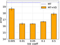
(a) classification error

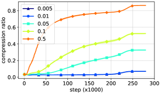
(b) sparsity curve

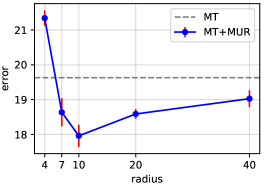
(c) classification error

Figure 2: (a), (b): Classification errors and weight sparsity curves of MT+VD w.r.t. different coefficients of the KLD of weights. (c): Classification errors of MT+MUR w.r.t. different values of the radius $r$. The dataset is CIFAR-10 with 1000 labels.

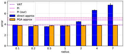
Figure 3: Classification errors of MUT w.r.t. different values of the radius $r$. For the PGA update of $x^{*}$, lr=0.3 and #steps=5. The dataset is SVHN with 1000 labels.

The coefficient of $D_{KL}\left(q_{\phi}(w)\|p(w)\right)$ in VBI

In Fig. 2a, we compare the errors of MT+VD w.r.t. different values of the coefficient of $D_{KL}\left(q_{\phi}(w)\|p(w)\right)$. Either too small or too large coefficients lead to inferior results since they correspond to too little or too much regularization on weights (Fig. 2b). However, even in the worst setting, MT+VD still outperforms MT. This again demonstrates the clear advantage of VBI in improving the robustness of models.

The radius $r$ in MUR

We now examine how the radius $r$ (Eq. 9) affects performance. If $r$ is too small, it is hard to find an adequate virtual point $x^{*}$ that the classifier $f$ is uncertain about. Moreover, as $x^{*}$ is very close to $x_{0}$, minimizing $\mathcal{L}_{\text{MUR}}$ causes $f$ to focus too much on ensuring the local flatness around $x_{0}$ instead of smoothing the area between $x_{0}$ and other data points, exacerbating the problem. By contrast, if $r$ is too big, $x^{*}$ is very different from $x_{0}$ and forcing consistency between these points may be inappropriate. Fig. 2c shows the error of MT+MUR on CIFAR-10 with 1000 labels as a function of $r$ ($r\in\{4,7,10,20,40\}$), which reflects the intuition presented: MT+MUR performs poorly when $r$ is too small (4) and worse than MT. When $r$ is too big (20, 40), the results are also not good. The optimal value of $r$ is 10. To make sure that this result is reasonable, we visualize the virtual samples w.r.t. different values of $r$ in the appendix.

Iterative approximations of $x^{*}$ in MUR

We investigate the performance of MT+MUR when iterative approximations of $x^{*}$ are used instead of the direct (linear) approximation (Eq. 10). We try both projected gradient ascent (PGA) and vanilla gradient ascent (GA) updates with the learning rate $\alpha$ varying in $\{0.1,1.0,10.0\}$ and the number of steps $s$ varying in $\{2,5,8\}$. We report results of the GA update in Fig. 4. . Clearly, larger $\alpha$ and $s$ both lead to smaller gradient norms of (real) data points ($\left\|g_{0}\right\|_{2}$ in Eq. 10) (Fig. 4b) and causes the model to learn faster early in training. However, if $\alpha$ is too large (10.0), the model performance tends to degrade over time. If $\alpha$ is too small (0.1), the results are usually suboptimal when $s$ is small (2) and many update steps are required to achieve good results (8). The best setting of the GA update is $(\alpha,s)$=(0.1,8) at which the error is 17.21, smaller than the error in case the direct approximation is used (17.96). (Results of the PGA update are presented in the appendix)

How important is finding the most uncertain virtual points?

We define a “random regularization” loss $\mathcal{L}_{\text{RR}}$ which has the same formula as $\mathcal{L}_{\text{MUR}}$ in Eq. 8 except that it acts on a random virtural points $\hat{x}^{*}$ instead of the most uncertain virtual point $x^{*}$. $\hat{x}^{*}$ is computed as follows:

$$\hat{x}^{*}=x_{0}+r\times\frac{u}{\left\|u\right\|_{2}}$$

where $u$ is a random vector/tensor whose elements are drawn independently from a standard Gaussian distribution $\mathcal{N}(0,1)$. Choosing $u$ like this ensures that $\hat{x}^{*}$ is sampled uniformly on the sphere of radius $r$ centered at $x_{0}$ (Muller 1959).

We compare MT+MUR (with the direct approximation of $x^{*}$) against MT combined with $\mathcal{L}_{\text{RR}}$ (denoted as MT+RR) w.r.t. different values of $r$ and show the results in Fig. 4c. The advantage of finding the most uncertain virtual points is clear when $r$ is not too big (e.g., 7 or 10). However, when $r$ becomes bigger and bigger (e.g., 20 or 40), this advantage disappears and MT+MUR performs similarly to MT+RR. We think the main reason is that when $r$ is big, the direct approximation of $x^{*}$ (Eq. 10) is no longer correct, making $x^{*}$ look more like a random point.

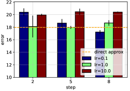
(a) classification error

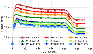
(b) $\left\|g_{0}\right\|_{2}$

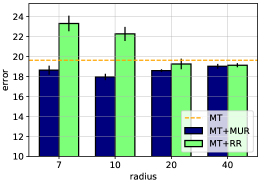
(c) classification error

Figure 4: (a), (b): Classification errors and gradient norm curves of MT+MUR with the GA update of $x^{*}$ w.r.t. different learning rates and numbers of steps. (c): Classification errors of MT+RR and MT+MUR w.r.t. different values of the radius $r$. The dataset is CIFAR-10 with 1000 labels.

Maximum Uncertainty Training (MUT)

It is important to know how well MUT performs compared to VAT and $\Pi$-model. To this end, we train MUT using the same settings for training $\Pi$-model on the SVHN dataset. The classification errors of MUT w.r.t. different values of the radius $r$ are shown in Fig. 3. At $r=0.5$, MUT with the direct approximation of $x^{*}$ (blue bars in Fig. 3) achieves the best error of 3.58$\pm$0.08 which is smaller the reported errors of VAT (Miyato et al. 2018) (3.86$\pm$0.11) and $\Pi$-model (Laine and Aila 2016) (4.82$\pm$0.17), and the error of our own implemented $\Pi$-model (5.18$\pm$0.13 in Table 2). However, the results become worse as $r$ increases. We believe the reason is that without the local smoothness term $\mathcal{L}_{\Pi\text{,cons}}(\theta,\theta_{\text{sg}})$ in MUT, the true most uncertain point $x^{*}$ usually lies closely to the real data point $x_{0}$ while the direct approximation $\tilde{x}^{*}=x_{0}+r\frac{g_{0}}{\left\|g_{0}\right\|_{2}}$ is always $r$ away from $x_{0}$. Therefore, if $r$ is not small enough, $\tilde{x}^{*}$ is no longer a correct approximation of $x^{*}$, which eliminates the smoothing effect of $\mathcal{L}_{\text{MUR}}$. Luckily, we can relax the distance constraint of $\tilde{x}^{*}$ by using the projected gradient ascent (PGA) update instead. To this end, the distance between $\tilde{x}^{*}$ and $x_{0}$ can be smaller than $r$, which gives us more freedom in choosing large $r$. This can be seen from Fig. 3 as the performance of MUT with the PGA approximation of $x^{*}$ is almost unaffected by $r$.

Related Work

Semi-supervised learning (SSL) is a long-established research area with diverse approaches (Chapelle, Scholkopf, and Zien 2006). Within the scope of this paper, we mainly focus on “consistency regularization” (CR) based methods. Details about other methods can be found in (van Engelen and Hoos 2019) and (Ouali, Hudelot, and Tami 2020). CR based methods aim at learning a smooth classifier by forcing it to give similar predictions for different perturbed inputs. There are many ways to define data perturbation but usually, the more distinct the two perturbations are, the smoother the classifier is. Standard methods such as Ladder Network (Rasmus et al. 2015), $\Pi$-model (Laine and Aila 2016) and Mean Teacher (Tarvainen and Valpola 2017) perturb data by applying small additive Gaussian noise and binary dropout to the input and hidden activations. VAT (Miyato et al. 2018) and VAdD (Park et al. 2018) use adversarial noise and adversarial dropout for perturbation, respectively. Both can be viewed as performing selective smoothing because they only flatten the input-output manifold along the direction that gives the largest variance in class prediction.

Data augmentation is another perturbation technique which is more effective than general noise injection in specific domains because it exploits the intrinsic domain structures (Xie et al. 2019). For example, augmenting image data with different color filters and affine transformations encourages the classifier to be insensitive to changes in color and shape (Cubuk et al. 2020). In case of text, using thesaurus (Zhang, Zhao, and LeCun 2015; Mueller and Thyagarajan 2016) and back translation (Sennrich, Haddow, and Birch 2016; Edunov et al. 2018) for augmentation makes the classifier robust to different paraphrases. These generalization capabilities cannot be obtained with general noise injections. However, data augmentation also comes with several limitations such as domain dependence and requirement for external knowledge not available in the training data.

Apart from data augmentation, standard CR based methods can also be improved by using additional smoothness-inducing objectives. For example, SNTG (Luo et al. 2018) introduces a new loss that forces every two data points with similar pseudo labels (up to a certain confidence level) to be close in the low-dimensional feature space. ICT (Verma et al. 2019) is a variant of MT which leverages MixUp (Zhang et al. 2017) to encourage linearity of the classifier. Holistic methods like MixMatch (Berthelot et al. 2019b), ReMixMatch (Berthelot et al. 2019a) and FixMatch (Sohn et al. 2020) combine different advanced techniques in SSL such as strong data augmentation (Cubuk et al. 2020), MixUp (Zhang et al. 2017), entropy minimization (Grandvalet and Bengio 2005) and pseudo labeling (Lee 2013) into a unified framework that performs well yet uses very few labeled data.

Conclusion

We have presented VBI and MUR - two general methods for improving SSL. We have demonstrated that combining existing CR based methods with VBI and MUR significantly reduces errors of these methods on various benchmark datasets. In the future, we would like to incorporate the likelihood of unlabeled data into VBI to learn a better posterior distribution of classifier’s weights. We also want to apply MUR to other machine learning problems that demand robustness and generalization.

Appendix A Appendix

Datasets

SVHN and CIFAR-10 have 10 output classes while CIFAR-100 has 100 output classes. All the datasets contain $32\times 32$ RGB images as input. Other details such as the numbers of training and testing samples for each dataset are provided in Table 5. Following previous works (Athiwaratkun et al. 2018; Laine and Aila 2016; Tarvainen and Valpola 2017), we preprocessed SVHN by normalizing the input images to zero mean and unit variance. For CIFAR-10 and CIFAR-100, we applied ZCA whitening to the input images. After the preprocessing step, we perturbed images with additive Gaussian noise, random translation, and random horizontal flip. Details of these transformations are given in Table 4.

Dataset	image size	#classes	#train	#test
SVHN	32$\times$32	10	73,257	26,032
CIFAR-10	32$\times$32	10	50,000	10,000
CIFAR-100	32$\times$32	100	50,000	10,000

Figure 5: Statistics about the datasets used in this paper.

Model Architecture

Following previous works (Athiwaratkun et al. 2018; Laine and Aila 2016; Tarvainen and Valpola 2017; Verma et al. 2019), we use a 13-layer CNN architecture (ConvNet-13) which is shown in Table 4. Batch Norm (Ioffe and Szegedy 2015) (momentum$=$0.999, epsilon$=$1e-8) and Leaky ReLU ($\alpha$$=$0.1) are applied to every convolutional layer of the ConvNet-13.

For models using variational dropout (VD), we simply replace the weight $w$ of every convolutional/fully-connected layer of the ConvNet-13 with two trainable parameters $\theta$ and $\log\sigma^{2}$. We also remove all dropout layers since they are unnecessary. Other settings are kept unchanged.

Layer	Hyperparameters
Input	32$\times$32 RGB image
Translationa	Random $\{\Delta x,\Delta y\}\sim[-4,4]$
Horizontal flipb	Random $p=0.5$
Gaussian noise	$\sigma=0.15$
Convolutional	128 filters, $3\times 3$, same padding
Convolutional	128 filters, $3\times 3$, same padding
Convolutional	128 filters, $3\times 3$, same padding
Max pooling	$2\times 2$
Dropout	$p=0.5$
Convolutional	256 filters, $3\times 3$, same padding
Convolutional	256 filters, $3\times 3$, same padding
Convolutional	256 filters, $3\times 3$, same padding
Max pooling	$2\times 2$
Dropout	$p=0.5$
Convolutional	512 filters, $3\times 3$, valid padding
Convolutional	256 filters, $1\times 1$, valid padding
Convolutional	128 filters, $1\times 1$, valid padding
Avg. pooling	$6\times 6$ $\rightarrow$ $1\times 1$ pixels
Fully connected	softmax, $128$ $\rightarrow$ $10$

Table 4: Architecture of the 13-layer CNN used in our paper, similar to those used in (Laine and Aila 2016; Tarvainen and Valpola 2017). The above settings are for CIFAR-10/CIFAR-100. For SVHN, two small changes are made ^a: $\{\Delta x,\Delta y\}\sim[-2,2]$ and ^b: no horizontal flip.

Training Settings

Here, we provide details about the settings we use for training our models. Unless otherwise specified, in all cases, when we say “ramp up to $a$”, it means increasing the value from 0 to $a$ during the first $t_{\text{ru}}$ training steps ($t_{\text{ru}}$ is a predefined ramp-up length) using a sigmoid-shaped function $e^{-5(1-x)^{2}}$ where $x\in[0,1]$. On the other hand, when we say “ramp down from $a$”, it means decreasing the value from $a$ to 0 during the last $t_{\text{rd}}$ training steps using another sigmoid-shaped function $1\text{\textminus}e^{-12.5x^{2}}$ where $x\in[0,1]$. The ramp-up and ramp-down functions are taken from (Tarvainen and Valpola 2017).

CIFAR-10 and CIFAR-100

We apply VD/MUR to MT (Tarvainen and Valpola 2017) and ICT (Verma et al. 2019) in the experiments on CIFAR-10/CIFAR-100. For both MT and ICT, the teacher updating momentum is fixed at 0.99. We use a Nesterov momentum optimizer with the momentum set to 0.9, the L2 weight decay coefficient set to 0.0001, and the learning rate ramped up to and ramped down from 0.1. The coefficient of the default consistency loss ($\lambda_{1}(t)$ in Eq. 7, main text) is ramped up to 10. In case VD is used, the coefficient of the KL divergence of weights ($\lambda_{2}(t)$ in Eq. 7, main text) is ramped up to 0.05. In case MUR is used, the coefficient of the MUR loss ($\lambda_{3}(t)$ in Eq. 7, main text) is ramped up to 4, the radius $r$ is set to 10 if the dataset is CIFAR-10 and 20 if the dataset is CIFAR-100. The total number of training steps is 280k. The ramp-up and ramp-down lengths are 10k and 80k steps, respectively. Each batch contains 100 samples with 25 labeled and 75 unlabeled.

SVHN

We apply VD/MUR to MT (Tarvainen and Valpola 2017) and $\Pi$-model (Laine and Aila 2016) in the experiments on SVHN. For MT, the teacher updating momentum is ramped up from 0.99 to 0.999 using a step function as in (Tarvainen and Valpola 2017). We train both models using a Nesterov momentum optimizer with the momentum fixed at 0.9. For MT, the L2 weight decay coefficient is set to 0.0002, the learning rate is ramped up to and ramped down from 0.03, $\lambda_{1}(t)$, $\lambda_{2}(t)$, and $\lambda_{3}(t)$ are ramped up to 12, 0.05, and 2, respectively. On the other hand, for $\Pi$-model, the L2 weight decay coefficient is set to 0.0001, the learning rate is ramped up to and ramped down from 0.01, $\lambda_{1}(t)$, $\lambda_{2}(t)$, and $\lambda_{3}(t)$ are ramped up to 10, 0.05, and 4, respectively. In case MUR is used, the radius $r$ is set to 10 for both models. The total number of training steps is 280k and the ramp-up length is 40k for both models. The ramp-down length is 0 for MT and 80k for $\Pi$-model. The batch size is 100 with 25 labeled and 75 unlabeled for both models.

Background on the Local Reparameterization Trick and Variational Dropout

The local reparameterization trick (Kingma, Salimans, and Welling 2015) is based on an observation that if $w\in\mathbb{R}^{M\times N}$ is a factorized Gaussian random variable with $w_{ij}\sim\mathcal{N}(w_{ij};\theta_{ij},\sigma_{ij}^{2})$ ($1\leq i\leq M$, $1\leq j\leq N$) then $z=w^{\top}x$ ($x\in\mathbb{R}^{M}$, $z\in\mathbb{R}^{N}$) is also a factorized Gaussian random variable with $z_{j}\sim\mathcal{N}(z_{i};\nu_{j},\omega_{j}^{2})$ and $\nu_{j}$, $\omega_{j}^{2}$ are given by:

$$\nu_{j}=\sum_{i=1}^{M}\theta_{ij}x_{i}\ \ \ \text{and}\ \ \ \omega_{j}^{2}=\sum_{i=1}^{M}\sigma_{ij}^{2}x_{i}^{2}$$

This trick allows us to convert weight ($w$) sampling into activation ($z$) sampling which is much faster and provides more stable gradient estimates. Using this trick, Kingma et. al. (Kingma, Salimans, and Welling 2015) further showed that VBI with a factorized Gaussian $q_{\phi}(w)$ was related to Gaussian dropout (Wang and Manning 2013) and derived a new generalization of Gaussian dropout called variational dropout (VD). To see the intuition behind this, we start from the original formula of Gaussian dropout which is given by:

$$z=\theta^{\top}(x\odot\xi)$$ (14)

where $\theta\sim\mathbb{R}^{M\times N}$ is a deterministic weight matrix; $\xi\in\mathbb{R}^{M}$ is a noise vector whose $\xi_{i}$ are sampled independently from $\mathcal{N}(\xi_{i};1,\alpha_{i})$. Inspired by the local reparameterization trick, we can write Eq. 14 as $z=w^{\top}x$ where $w\in\mathbb{R}^{M\times N}$ is a random weight matrix obtained by perturbing $\theta$ with the multiplicative noise $\xi$. We can easily show that $w_{ij}$ has a Gaussian distribution $\mathcal{N}(w;\theta_{ij},\alpha_{i}\theta_{ij}^{2})$. In VBI, this distribution corresponds to the variational posterior distribution $q_{\phi_{ij}}(w_{ij})$ of an individual weight $w_{ij}$, hence, Eq. 14 is referred to as variational dropout. The main difference between Gaussian dropout and variational dropout is that in Gaussian dropout, the dropout rate $\alpha$ is fixed while in variational dropout, $\alpha$ can be learned to adapt to the data via optimizing the ELBO w.r.t. $w$ (Eq. 6, main text).

The dropout rate $\alpha$ can also be used to compute the model’s sparsity. Based on a theoretical result showing that Gaussian dropout with $\alpha=\frac{p}{1-p}$ is equivalent to binary dropout with the dropout rate $p$ (Srivastava et al. 2014), we remove a weight component $w_{ij}$ (by setting its value to 0) if $\log\alpha_{ij}\leq 3$ as this corresponds to $p_{ij}\geq 0.95$.

Why is VD chosen in this work?

In order to train a large scale Bayesian neural network (BNN) with the loss in Eq. 7, main text, it is important to choose a VBI method that supports efficient sampling of the random weights $w$. We choose VD because it satisfies the above requirement and is flexible enough to be applied to different network architectures. However, we note that our proposed method is not limited to VD, and any VBI method more advanced than VD can be used as a replacement. We discuss some possible alternatives below, real implementations will be left for future work.

One promising alternative to train large scale BNNs is sampling-free VI (Haußmann, Hamprecht, and Kandemir 2020; Hernández-Lobato and Adams 2015; Wu et al. 2018) which leverages moment propagation to derive an analytical expression for the reconstruction term of the ELBO. To the best of our knowledge, the most recent advance along this line of works is Deterministic Variational Inference (DVI) (Wu et al. 2018). However, this method only supports networks with Heaviside or ReLU activation functions, and in case of classification, it can only approximate the reconstruction term (Appdx. B4 in (Wu et al. 2018)).

Another interesting approach is leveraging natural gradient with adaptive weight noise (Zhang et al. 2018; Khan et al. 2018) to learn the variational distribution of weights. This approach has several advantages: i) it can be easily integrated into existing optimizers such as Adam, and ii) it supports the weight prior with different structures. However, it is not clear how the natural gradient can be computed for our model.

In VBI, the form of the prior distribution $p(w)$ is also important as it affects how well the weights can be compressed (Louizos, Ullrich, and Welling 2017; Louizos, Welling, and Kingma 2017; Neklyudov et al. 2017) and how well $q_{\phi}(w)$ can match the true posterior. However, choosing a good prior is not the main focus of this paper so we simply choose $p(w)$ to be the log-uniform prior, which is the default prior for VD.

Derivation of the direct approximation of $x^{*}$ in Eq. 10, main text

Recall that in Eq. 9, main text, $x^{*}$ is defined as follows:

$$x^{*}=\underset{x}{\text{argmax }}H(p(y|x))\ \ \ \text{s.t.}\ \ \ \left\|x-x_{0}\right\|_{2}\leq r$$ (15)

The above objective may have multiple local optima (w.r.t. $x$). To simplify the problem, we replace $f(x)=H(p(y|x))$ with its linear approximation derived from the first-order Taylor expansion:

$$f(x)\approx f(x_{0})+{f^{\prime}(x_{0})}^{\top}(x-x_{0})$$ (16)

This approximation is usually a lower bound of $H(p(y|x))$ (see the next section for an explanation). Thus, instead of solving the optimization problem in Eq. 15, we solve the following problem:

$$x^{*}\approx\underset{x}{\text{argmax }}f(x_{0})+{f^{\prime}(x_{0})}^{\top}(x-x_{0})\ \ \ \text{s.t.}\ \ \ \left\|x-x_{0}\right\|_{2}\leq r$$ (17)

With this approximation, the optimization problem in Eq. 17 becomes a convex minimization problem w.r.t. $x$, which means a solution, if exists, is unique. Using the method of Lagrange multipliers, we can rewrite Eq. 17 as follows:

$$\max_{x,\lambda}\mathcal{O}(x,\lambda)\triangleq\ f(x_{0})+{f^{\prime}(x_{0})}^{\top}(x-x_{0})-$$

$$\lambda\left(\left\|x-x_{0}\right\|_{2}-r\right)\ \ \ \text{s.t.}\ \ \ \lambda>0$$ (18)

By setting the derivation of $\mathcal{O}(x,\lambda)$ w.r.t. $x_{i}$ (the $i$-th component of $x$) $\forall i\in\{1,...,D\}$ to $0$, we have:

$$\frac{\partial\mathcal{O}}{\partial x_{i}}={f^{\prime}(x_{0})}_{i}-\lambda\frac{x_{i}-x_{0,i}}{\left\|x-x_{0}\right\|_{2}}=0$$

$$\Leftrightarrow x_{i}-x_{0,i}=\frac{{f^{\prime}(x_{0})}_{i}\left\|x-x_{0}\right\|_{2}}{\lambda}=\frac{g_{0,i}\left\|x-x_{0}\right\|_{2}}{\lambda}$$ (19)

where $g_{0,i}={f^{\prime}(x_{0})}_{i}$. Similarly, by setting the derivation of $\mathcal{O}(x,\lambda)$ w.r.t. $\lambda$ to 0, we have:

$$\frac{\partial\mathcal{O}}{\partial\lambda}=\left\|x-x_{0}\right\|_{2}-r=0$$

$$\Leftrightarrow \left\|x-x_{0}\right\|_{2}=r$$

$$\Leftrightarrow \sqrt{\sum_{i=1}^{D}\left(x_{i}-x_{0,i}\right)^{2}}=r$$ (20)

Substituting $x_{i}-x_{0,i}$ from Eq. 19 into Eq. 20, we have:

$$\frac{\left\|x-x_{0}\right\|_{2}}{\lambda}\sqrt{\sum_{i=1}^{D}g_{0,i}^{2}}=r$$

$$\Leftrightarrow \lambda=\frac{\left\|x-x_{0}\right\|_{2}\left\|g_{0}\right\|_{2}}{r}$$ (21)

We can see that $\lambda>0$ $\forall x\neq x_{0}$. Applying it to Eq. 19, we have:

$$x_{i}-x_{0,i} =\frac{g_{0,i}\left\|x-x_{0}\right\|_{2}r}{\left\|x-x_{0}\right\|_{2}\left\|g_{0}\right\|_{2}}$$

$$=r\frac{g_{0,i}}{\left\|g_{0}\right\|_{2}}$$

which means $x=x_{0}+r\frac{g_{0}}{\left\|g_{0}\right\|_{2}}$.

Lower bound property of the linear approximation of $H(p(y|x))$

The second-order Taylor expansion of $f(x)=H(p(y|x))$ is given by:

$$f(x)\approx f(x_{0})+{f^{\prime}(x_{0})}^{\top}(x-x_{0})+\frac{1}{2}{(x-x_{0})}^{\top}\mathcal{H}(x_{0})(x-x_{0})$$

where $\mathcal{H}(x_{0})$ denotes the Hessian matrix of $H(p(y|x))$ at $x_{0}$. During training, $H(p(y|x_{0}))$ is usually close to 0 as the model becomes more certain about the label of $x_{0}$ (or we can encourage that by penalizing $H(p(y|x_{0}))$ explicitly (Grandvalet and Bengio 2005)). Thus, $x_{0}$ tends to be a local minimum of $H(p(y|x))$ and $\mathcal{H}(x_{0})$ is likely to be positive semi-definite. This suggests that $f(x)$ is usually greater than $f(x_{0})+{f^{\prime}(x_{0})}^{\top}(x-x_{0})$ in the neighborhood of $x_{0}$.

Projected gradient ascent for the original constrained optimization problem in Eq. 9, main text

A common way to solve the constrained optimization problem in Eq. 9, main text in an iterative manner is using projected gradient ascent. The approximation of $x^{*}$ at step $t+1$ ($0\leq t\leq T$) is given by:

$$\tilde{x}_{t+1} =x_{t}+\alpha\frac{\partial H(p(y|x_{t}))}{\partial x_{t}}$$ (22)

$$x_{t+1} =\underset{x,\left\|x-x_{0}\right\|_{2}\leq r}{\text{argmin }}\frac{1}{2}\left\|x-\tilde{x}_{t+1}\right\|_{2}^{2}$$ (23)

where $\alpha\in\mathbb{R}^{+}$ is the learning rate. Note that the projection step (Eq. 23) is a convex minimization problem. It achieves the minimum at $\tilde{x}_{t+1}$ if $\left\|\tilde{x}_{t+1}-x_{0}\right\|_{2}\leq r$ and at $x_{0}+r\frac{\tilde{x}_{t+1}-x_{0}}{\left\|\tilde{x}_{t+1}-x_{0}\right\|_{2}}$ if $\left\|\tilde{x}_{t+1}-x_{0}\right\|_{2}>r$. Thus, $x_{t+1}$ in Eq. 23 can be rewritten as follows:

$$x_{t+1}=\begin{cases}\tilde{x}_{t+1}&\text{if}\ \left\|\tilde{x}_{t+1}-x_{0}\right\|_{2}\leq r\\ x_{0}+r\frac{\tilde{x}_{t+1}-x_{0}}{\left\|\tilde{x}_{t+1}-x_{0}\right\|_{2}}&\text{otherwise}\end{cases}$$

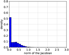
(a) MT

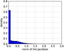
(b) MT+VD

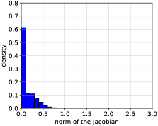
(c) MT+MUR

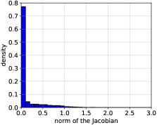
(d) MT+VD+MUR

Figure 6: Sensitivity histograms of MT and its variants trained on CIFAR-10 with 1000 labels.

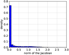
(a) ICT

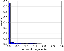
(b) ICT+VD

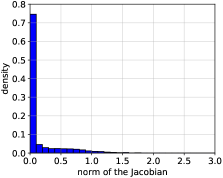
(c) ICT+MUR

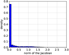
(d) ICT+VD+MUR

Figure 7: Sensitivity histograms of ICT and its variants trained on CIFAR-10 with 1000 labels.

Gradient ascent for the Lagrangian relaxation problem in Eq. 11, main text

The Lagrangian relaxation of the constrained optimization problem in Eq. 9, main text is given by:

$$\max_{x,\lambda}\mathcal{F}(x,\lambda)\triangleq f(x)-\lambda\left(\left\|x-x_{0}\right\|_{2}-r\right)\ \ \ \text{s.t.}\ \ \ \lambda>0$$ (24)

where $f(x)=H(p(y|x))$.

One can think of Eq. 24 as a two-step optimization procedure: First, we maximize $\mathcal{F}(x,\lambda)$ w.r.t. $\lambda$ to find the optimal $\lambda^{*}$ as a function of $x$. Then, we maximize $\mathcal{F}(x,\lambda^{*})$ w.r.t. $x$ using $\lambda^{*}$ obtained in the previous step.

However, in the first step, we maximize the approximate of $\mathcal{F}(x,\lambda)$ given in Eq. 18 instead of $\mathcal{F}(x,\lambda)$. This yields $\lambda^{*}(x)$ with similar formula to the one in Eq. 21:

$$\lambda^{*}(x)=\frac{\left\|x-x_{0}\right\|_{2}\left\|g_{0}\right\|_{2}}{r}$$ (25)

In the second step, we solve the following optimization problem:

$$x^{*}= \underset{x}{\text{argmax }}\mathcal{F}(x)\triangleq f(x)-\frac{\left\|x-x_{0}\right\|_{2}\left\|g_{0}\right\|_{2}}{r}\left(\left\|x-x_{0}\right\|_{2}-r\right)$$

$x^{*}$ can be updated iteratively using vanilla gradient ascent:

$$x_{t+1}=x_{t}+\alpha\frac{\partial\mathcal{F}(x)}{\partial x}$$

with $\frac{\partial\mathcal{F}(x)}{\partial x}$ computed as follows:

$$\frac{\partial\mathcal{F}(x)}{\partial x}=f^{\prime}(x)-\frac{\left\|g_{0}\right\|_{2}(x-x_{0})}{r}\left(2-\frac{r}{\left\|x-x_{0}\right\|_{2}}\right)$$

Sensitivity histograms of MT, ICT and their variants

The sensitivity histograms of MT, ICT and their variants are shown in Figs. 6, 7. It is clear that using VD and MUR significantly reduce the classifier’s sensitivity.

Visualization of virtual samples

To have a better understanding of how virtual samples w.r.t. different radiuses look like, we show their images in Fig. 8 after normalizing the pixel values to [0, 1]. Since the minimum/maximum pixel values of ZCA whitened CIFAR-10 images are around -30/30, normalization scales the noise intensity by a factor of 1/60. This is the reason why we cannot see much difference between the virtual samples at $r=10$ and the input samples.

Figure 8: Visualization of virtual samples generated by MT+MUR w.r.t. different radiuses. The model is trained on ZCA whitened CIFAR-10 images.

To improve visualization, we generate virtual samples for unwhitened images. The perturbed images are clipped in [0, 1] and are shown in Fig. 9. It is clear that when $r$ is small (4, 7), the perturbed images look quite similar to the input images. By contrast, when $r$ is big (20, 40), most of the information is lost and the perturb images look very noisy. A reasonable value of $r$ is 10.

Figure 9: Visualization of virtual samples generated by MT+MUR w.r.t. different radiuses. The model is trained on ZCA whitened CIFAR-10 images.

However, since our models are trained on ZCA whitened images, the visualization in Fig. 9 may not be correct. We address this issue by training a MT+MUR on unwhitened images. From Fig. 10, we see that only object features critical for class prediction are perturbed. Other less important features like background usually remain unchanged. It suggests that MT+MUR correctly find examples with maximum uncertainty based on its learned class-intrinsic features.

Figure 10: Visualization of virtual samples generated by MT+MUR w.r.t. different radiuses. The model is trained on unwhitened CIFAR-10 images.

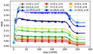
(a) MUR

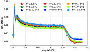
(b) consistency loss

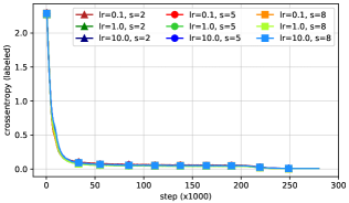
(c) cross-entropy loss

Figure 11: Loss curves of MT+MUR with the vanilla gradient ascent update of $x^{*}$ w.r.t. different learning rates and numbers of steps. The dataset is CIFAR-10 with 1000 labels.

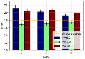
(a) classification error

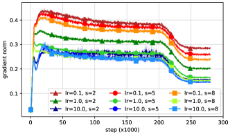
(b) $\left\|g_{0}\right\|$

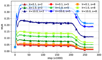
(c) MUR

Figure 12: Results of MT+MUR with the projected gradient ascent update of $x^{*}$ w.r.t. different learning rates and numbers of steps. The dataset is CIFAR-10 with 1000 labels.

More results of MT+MUR with iterative approximations of $x^{*}$

Fig. 11 shows the loss curves of MT+MUR with the vanilla gradient ascent (GA) update of $x^{*}$. While the MUR loss is affected by different settings of the learning rate $\alpha$ and the number of steps $s$, the consistency and cross-entropy losses remain almost unchanged. In addition, larger $\alpha$ and larger $s$ both lead to larger MUR losses since they encourage the model to find $x^{*}$ farther from $x_{0}$.

MT+MUR with the projected gradient ascent (PGA) update

Results of MT+MUR with the projected gradient ascent (PGA) update of $x^{*}$ are shown in Fig. 12. Overall, the dynamics of the PGA update is very similar to that of the GA update.

We also provide a direct comparison of the classification error between GA and PGA for every setting of $(\alpha,s)$ in Fig. 13. We see that when $\alpha=0.1$, GA performs better than PGA but when $\alpha=1.0$, PGA is better. The best result given by PGA is 16.81$\pm$0.31 at $\alpha=1.0$ and $s=2$.

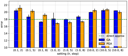
Figure 13: Comparison between the GA and PGA updates of $x^{*}$ on different settings of (learning rate, number of steps).

Combining VBI and MUR with FixMatch

Figure 14: Virtual samples generated by FM+MUR. The model is trained on strongly-augmented CIFAR-10 images.

FixMatch (FM) (Sohn et al. 2020) is currently one of the state-of-the-art CR based methods that use strong data augmentation (Cubuk et al. 2019, 2020). Its loss function is given by:

$$\mathcal{L}_{\text{FM}}(\theta)=\ \mathbb{E}_{(x_{l},y_{l})\sim\mathcal{D}_{l}}\left[-\log p(y_{l}|x_{l},\theta)\right]+$$

$$\lambda\mathbb{E}_{x_{u}\sim\mathcal{D}_{u}}\left[-1_{p(\tilde{y}|x_{u},\theta)>\tau}\log p(\tilde{y}|\mathcal{A}(x_{u}),\theta)\right]$$ (26)

where $\mathcal{A}(x_{u})$ denotes the strongly-augmented version of $x_{u}$; $\tilde{y}$ is the pseudo label of $x_{u}$ which satisfies that $\tilde{y}=\underset{k}{\text{argmax }}p(k|x_{u})$; $\tau$ is a confidence threshold.

Since the loss function of FixMatch in Eq. 26 also has the form $\mathcal{L}_{\text{xent,}l}(\theta)+\lambda(t)\mathcal{L}_{\text{cons}}(\theta,\cdot)$, we can integrate VBI and MUR into this model. The loss function of FM+VBI is:

$$\mathcal{L}_{\text{FM+VBI}}(\phi)=$$

$$\mathbb{E}_{w\sim q_{\phi}(w)}\left[\mathbb{E}_{(x_{l},y_{l})\sim\mathcal{D}_{l}}\left[-\log p(y_{l}|x_{l},w)\right]\right]+$$

$$\lambda_{1}\mathbb{E}_{w\sim q_{\phi}(w)}\left[\mathbb{E}_{x_{u}\sim\mathcal{D}_{u}}\left[-1_{p(\tilde{y}|x_{u},\theta)>\tau}\log p(\tilde{y}|\mathcal{A}(x_{u}),w)\right]\right]+$$

$$\lambda_{2}D_{KL}(q_{\phi}(w)\|p(w))$$

with a note that in the indicator function, we use the mean network $f_{\theta}$ to compute $p(\tilde{y}|x_{u},\theta)$.

And the loss function of FM+MUR is:

$$\mathcal{L}_{\text{FM+MUR}}(\phi)=\ \mathbb{E}_{(x_{l},y_{l})\sim\mathcal{D}_{l}}\left[-\log p(y_{l}|x_{l},w)\right]+$$

$$\lambda\mathbb{E}_{x_{u}\sim\mathcal{D}_{u}}\left[-1_{p(\tilde{y}|x_{u},\theta)>\tau}\log p(\tilde{y}|\mathcal{A}^{*}(x_{u}),w)\right]$$

where $\mathcal{A^{*}}(x_{u})$ is the MUR virtual point of $\mathcal{A}(x_{u})$ found by optimizing the following objective:

$$\mathcal{A}^{*}(x_{u})=\underset{x}{\text{argmax }}H(p(y|x))\ \ \ \text{s.t.}\ \ \ \|x-\mathcal{A}(x_{u})\|\leq r$$ (27)

In our experiments, we observed that FM+VD gives the same results as FM, which suggests that weight perturbation has almost no contribution on generalization when strong data augmentation is available. FM+MUR, however, is much worse than FM. For example, on CIFAR-10 with 250 labels, FM achieves an average error of 5.07 while FM+MUR can only achieve an average error of 13.45. We guess the problem is that the class predictions for strongly-augmented data is much more inconsistent and inaccurate compared to the class predictions for normal data. Thus, the MUR optimization problem in Eq. 27 is often ill-posed and may not return desirable results. We can check that by visualizing the virtual samples for strongly-augmented data in Fig. 14.

References

- Alain and Bengio (2014) Alain, G.; and Bengio, Y. 2014. What regularized auto-encoders learn from the data-generating distribution. The Journal of Machine Learning Research 15(1): 3563–3593.
- Athiwaratkun et al. (2018) Athiwaratkun, B.; Finzi, M.; Izmailov, P.; and Wilson, A. G. 2018. There are many consistent explanations of unlabeled data: Why you should average. arXiv preprint arXiv:1806.05594 .
- Bachman, Alsharif, and Precup (2014) Bachman, P.; Alsharif, O.; and Precup, D. 2014. Learning with pseudo-ensembles. In Advances in Neural Information Processing Systems, 3365–3373.
- Berthelot et al. (2019a) Berthelot, D.; Carlini, N.; Cubuk, E. D.; Kurakin, A.; Sohn, K.; Zhang, H.; and Raffel, C. 2019a. ReMixMatch: Semi-Supervised Learning with Distribution Alignment and Augmentation Anchoring. arXiv preprint arXiv:1911.09785 .
- Berthelot et al. (2019b) Berthelot, D.; Carlini, N.; Goodfellow, I.; Papernot, N.; Oliver, A.; and Raffel, C. A. 2019b. Mixmatch: A holistic approach to semi-supervised learning. In Advances in Neural Information Processing Systems, 5050–5060.
- Blundell et al. (2015) Blundell, C.; Cornebise, J.; Kavukcuoglu, K.; and Wierstra, D. 2015. Weight uncertainty in neural networks. In Proceedings of the 32nd International Conference on International Conference on Machine Learning-Volume 37, 1613–1622.
- Chapelle, Scholkopf, and Zien (2006) Chapelle, O.; Scholkopf, B.; and Zien, A. 2006. Semi-Supervised Learning. MIT Press.
- Cubuk et al. (2019) Cubuk, E. D.; Zoph, B.; Mane, D.; Vasudevan, V.; and Le, Q. V. 2019. Autoaugment: Learning augmentation strategies from data. In Proceedings of the IEEE conference on computer vision and pattern recognition, 113–123.
- Cubuk et al. (2020) Cubuk, E. D.; Zoph, B.; Shlens, J.; and Le, Q. V. 2020. Randaugment: Practical automated data augmentation with a reduced search space. In Proceedings of the IEEE/CVF Conference on Computer Vision and Pattern Recognition Workshops, 702–703.
- Edunov et al. (2018) Edunov, S.; Ott, M.; Auli, M.; and Grangier, D. 2018. Understanding Back-Translation at Scale. In Proceedings of the 2018 Conference on Empirical Methods in Natural Language Processing, 489–500.
- Farnia and Tse (2016) Farnia, F.; and Tse, D. 2016. A minimax approach to supervised learning. In Advances in Neural Information Processing Systems, 4240–4248.
- Globerson and Roweis (2006) Globerson, A.; and Roweis, S. 2006. Nightmare at test time: robust learning by feature deletion. In Proceedings of the 23rd international conference on Machine learning, 353–360.
- Goodfellow, Shlens, and Szegedy (2014) Goodfellow, I. J.; Shlens, J.; and Szegedy, C. 2014. Explaining and harnessing adversarial examples. arXiv preprint arXiv:1412.6572 .
- Grandvalet and Bengio (2005) Grandvalet, Y.; and Bengio, Y. 2005. Semi-supervised Learning by Entropy Minimization. In Advances in neural information processing systems, 529–536.
- Grathwohl et al. (2019) Grathwohl, W.; Wang, K.-C.; Jacobsen, J.-H.; Duvenaud, D.; Norouzi, M.; and Swersky, K. 2019. Your Classifier is Secretly an Energy Based Model and You Should Treat it Like One. arXiv preprint arXiv:1912.03263 .
- Graves (2011) Graves, A. 2011. Practical variational inference for neural networks. In Advances in neural information processing systems, 2348–2356.
- Haußmann, Hamprecht, and Kandemir (2020) Haußmann, M.; Hamprecht, F. A.; and Kandemir, M. 2020. Sampling-Free Variational Inference of Bayesian Neural Networks by Variance Backpropagation. In Uncertainty in Artificial Intelligence, 563–573. PMLR.
- Hernández-Lobato and Adams (2015) Hernández-Lobato, J. M.; and Adams, R. 2015. Probabilistic backpropagation for scalable learning of bayesian neural networks. In International Conference on Machine Learning, 1861–1869.
- Hinton and von Cramp (1993) Hinton, G.; and von Cramp, D. 1993. Keeping neural networks simple by minimising the description length of weights. In Proceedings of COLT-93, 5–13.
- Hochreiter and Schmidhuber (1997) Hochreiter, S.; and Schmidhuber, J. 1997. Flat minima. Neural Computation 9(1): 1–42.
- Honkela and Valpola (2004) Honkela, A.; and Valpola, H. 2004. Variational learning and bits-back coding: an information-theoretic view to Bayesian learning. IEEE transactions on Neural Networks 15(4): 800–810.
- Ioffe and Szegedy (2015) Ioffe, S.; and Szegedy, C. 2015. Batch normalization: Accelerating deep network training by reducing internal covariate shift. arXiv preprint arXiv:1502.03167 .
- Izmailov et al. (2018) Izmailov, P.; Podoprikhin, D.; Garipov, T.; Vetrov, D.; and Wilson, A. G. 2018. Averaging weights leads to wider optima and better generalization. arXiv preprint arXiv:1803.05407 .
- Khan et al. (2018) Khan, M. E.; Nielsen, D.; Tangkaratt, V.; Lin, W.; Gal, Y.; and Srivastava, A. 2018. Fast and scalable bayesian deep learning by weight-perturbation in adam. arXiv preprint arXiv:1806.04854 .
- Kingma, Salimans, and Welling (2015) Kingma, D. P.; Salimans, T.; and Welling, M. 2015. Variational dropout and the local reparameterization trick. In Advances in neural information processing systems, 2575–2583.
- Kingma and Welling (2013) Kingma, D. P.; and Welling, M. 2013. Auto-encoding Variational Bayes. arXiv preprint arXiv:1312.6114 .
- Laine and Aila (2016) Laine, S.; and Aila, T. 2016. Temporal ensembling for semi-supervised learning. arXiv preprint arXiv:1610.02242 .
- Lee (2013) Lee, D.-H. 2013. Pseudo-label: The simple and efficient semi-supervised learning method for deep neural networks. In Workshop on challenges in representation learning, ICML, volume 3, 2.
- Loshchilov and Hutter (2016) Loshchilov, I.; and Hutter, F. 2016. SGDR: Stochastic gradient descent with warm restarts. arXiv preprint arXiv:1608.03983 .
- Louizos, Ullrich, and Welling (2017) Louizos, C.; Ullrich, K.; and Welling, M. 2017. Bayesian compression for deep learning. In Advances in neural information processing systems, 3288–3298.
- Louizos, Welling, and Kingma (2017) Louizos, C.; Welling, M.; and Kingma, D. P. 2017. Learning Sparse Neural Networks through Regularization. arXiv preprint arXiv:1712.01312 .
- Luo et al. (2018) Luo, Y.; Zhu, J.; Li, M.; Ren, Y.; and Zhang, B. 2018. Smooth Neighbors on Teacher Graphs for Semi-Supervised Learning. In 2018 IEEE/CVF Conference on Computer Vision and Pattern Recognition, 8896–8905. IEEE.
- Madry et al. (2017) Madry, A.; Makelov, A.; Schmidt, L.; Tsipras, D.; and Vladu, A. 2017. Towards deep learning models resistant to adversarial attacks. arXiv preprint arXiv:1706.06083 .
- Miyato et al. (2018) Miyato, T.; Maeda, S.-i.; Koyama, M.; and Ishii, S. 2018. Virtual adversarial training: a regularization method for supervised and semi-supervised learning. IEEE transactions on pattern analysis and machine intelligence 41(8): 1979–1993.
- Molchanov, Ashukha, and Vetrov (2017) Molchanov, D.; Ashukha, A.; and Vetrov, D. 2017. Variational dropout sparsifies deep neural networks. In Proceedings of the 34th International Conference on Machine Learning-Volume 70, 2498–2507. JMLR. org.
- Mueller and Thyagarajan (2016) Mueller, J.; and Thyagarajan, A. 2016. Siamese recurrent architectures for learning sentence similarity. In Proceedings of the Thirtieth AAAI Conference on Artificial Intelligence, 2786–2792.
- Muller (1959) Muller, M. E. 1959. A note on a method for generating points uniformly on n-dimensional spheres. Communications of the ACM 2(4): 19–20.
- Neklyudov et al. (2017) Neklyudov, K.; Molchanov, D.; Ashukha, A.; and Vetrov, D. P. 2017. Structured bayesian pruning via log-normal multiplicative noise. In Advances in Neural Information Processing Systems, 6775–6784.
- Novak et al. (2018) Novak, R.; Bahri, Y.; Abolafia, D. A.; Pennington, J.; and Sohl-Dickstein, J. 2018. Sensitivity and generalization in neural networks: an empirical study. arXiv preprint arXiv:1802.08760 .
- Ouali, Hudelot, and Tami (2020) Ouali, Y.; Hudelot, C.; and Tami, M. 2020. An Overview of Deep Semi-Supervised Learning. arXiv preprint arXiv:2006.05278 .
- Park et al. (2018) Park, S.; Park, J.; Shin, S.-J.; and Moon, I.-C. 2018. Adversarial dropout for supervised and semi-supervised learning. In Thirty-Second AAAI Conference on Artificial Intelligence.
- Qiao et al. (2018) Qiao, S.; Shen, W.; Zhang, Z.; Wang, B.; and Yuille, A. 2018. Deep co-training for semi-supervised image recognition. In Proceedings of the european conference on computer vision (eccv), 135–152.
- Rasmus et al. (2015) Rasmus, A.; Berglund, M.; Honkala, M.; Valpola, H.; and Raiko, T. 2015. Semi-supervised learning with ladder networks. In Advances in neural information processing systems, 3546–3554.
- Rezende, Mohamed, and Wierstra (2014) Rezende, D. J.; Mohamed, S.; and Wierstra, D. 2014. Stochastic Backpropagation and Approximate Inference in Deep Generative Models. arXiv preprint arXiv:1401.4082 .
- Rifai et al. (2011) Rifai, S.; Vincent, P.; Muller, X.; Glorot, X.; and Bengio, Y. 2011. Contractive Auto-Encoders: Explicit Invariance During Feature Extraction. In Proceedings of the 28th International Conference on International Conference on Machine Learning, 833–840. Omnipress.
- Sajjadi, Javanmardi, and Tasdizen (2016) Sajjadi, M.; Javanmardi, M.; and Tasdizen, T. 2016. Regularization with stochastic transformations and perturbations for deep semi-supervised learning. In Advances in Neural Information Processing Systems, 1163–1171.
- Sennrich, Haddow, and Birch (2016) Sennrich, R.; Haddow, B.; and Birch, A. 2016. Improving Neural Machine Translation Models with Monolingual Data. In Proceedings of the 54th Annual Meeting of the Association for Computational Linguistics (Volume 1: Long Papers), 86–96.
- Sinha, Namkoong, and Duchi (2017) Sinha, A.; Namkoong, H.; and Duchi, J. 2017. Certifying some distributional robustness with principled adversarial training. arXiv preprint arXiv:1710.10571 .
- Sohn et al. (2020) Sohn, K.; Berthelot, D.; Li, C.-L.; Zhang, Z.; Carlini, N.; Cubuk, E. D.; Kurakin, A.; Zhang, H.; and Raffel, C. 2020. Fixmatch: Simplifying semi-supervised learning with consistency and confidence. arXiv preprint arXiv:2001.07685 .
- Srivastava et al. (2014) Srivastava, N.; Hinton, G.; Krizhevsky, A.; Sutskever, I.; and Salakhutdinov, R. 2014. Dropout: a simple way to prevent neural networks from overfitting. The journal of machine learning research 15(1): 1929–1958.
- Szegedy et al. (2013) Szegedy, C.; Zaremba, W.; Sutskever, I.; Bruna, J.; Erhan, D.; Goodfellow, I.; and Fergus, R. 2013. Intriguing properties of neural networks. arXiv preprint arXiv:1312.6199 .
- Tarvainen and Valpola (2017) Tarvainen, A.; and Valpola, H. 2017. Mean teachers are better role models: Weight-averaged consistency targets improve semi-supervised deep learning results. In Advances in Neural Information Processing Systems, 1195–1204.
- van Engelen and Hoos (2019) van Engelen, J. E.; and Hoos, H. H. 2019. A survey on semi-supervised learning. Machine Learning 1–68.
- Verma et al. (2019) Verma, V.; Lamb, A.; Kannala, J.; Bengio, Y.; and Lopez-Paz, D. 2019. Interpolation consistency training for semi-supervised learning. arXiv preprint arXiv:1903.03825 .
- Wang and Manning (2013) Wang, S.; and Manning, C. 2013. Fast dropout training. In international conference on machine learning, 118–126.
- Wu et al. (2018) Wu, A.; Nowozin, S.; Meeds, E.; Turner, R. E.; Hernández-Lobato, J. M.; and Gaunt, A. L. 2018. Deterministic variational inference for robust bayesian neural networks. arXiv preprint arXiv:1810.03958 .
- Xie et al. (2019) Xie, Q.; Dai, Z.; Hovy, E.; Luong, M.-T.; and Le, Q. V. 2019. Unsupervised data augmentation for consistency training .
- Zhang et al. (2018) Zhang, G.; Sun, S.; Duvenaud, D.; and Grosse, R. 2018. Noisy natural gradient as variational inference. In International Conference on Machine Learning, 5852–5861.
- Zhang et al. (2017) Zhang, H.; Cisse, M.; Dauphin, Y. N.; and Lopez-Paz, D. 2017. mixup: Beyond empirical risk minimization. arXiv preprint arXiv:1710.09412 .
- Zhang, Zhao, and LeCun (2015) Zhang, X.; Zhao, J.; and LeCun, Y. 2015. Character-level convolutional networks for text classification. In Advances in neural information processing systems, 649–657.