Gaia Early Data Release 3: Structure and properties of the Magellanic Clouds

Abstract

Context. This work is part of the Gaia Data Processing and Analysis Consortium (DPAC) papers published with the Gaia Early Data Release 3 (EDR3). It is one of the demonstration papers aiming to highlight the improvements and quality of the newly published data by applying them to a scientific case.

Aims. We use the Gaia  EDR3 data to study the structure and kinematics of the Magellanic Clouds. The large distance to the Clouds is a challenge for the Gaia astrometry. The Clouds lie at the very limits of the usability of the Gaia data, which makes the Clouds an excellent case study for evaluating the quality and properties of the Gaia data.

Methods. The basis of our work are two samples selected to provide a representation as clean as possible of the stars of the Large Magellanic Cloud (LMC) and the Small Magellanic Cloud (SMC). The selection used criteria based on position, parallax, and proper motions to remove foreground contamination from the Milky Way, and allowed the separation of the stars of both Clouds. From these two samples we defined a series of subsamples based on cuts in the colour-magnitude diagram; these subsamples were used to select stars in a common evolutionary phase and can also be used as approximate proxies of a selection by age.

Results. We compared the Gaia Data Release 2 (DR2) and Gaia  EDR3 performances in the study of the Magellanic Clouds and show the clear improvements in precision and accuracy in the new release. We also show that the systematics still present in the data make the determination of the 3D geometry of the LMC a difficult endeavour; this is at the very limit of the usefulness of the Gaia  EDR3 astrometry, but it may become feasible with the use of additional external data.

We derive radial and tangential velocity maps and global profiles for the LMC for the several subsamples we defined. To our knowledge, this is the first time that the two planar components of the ordered and random motions are derived for multiple stellar evolutionary phases in a galactic disc outside the Milky Way, showing the differences between younger and older phases. We also analyse the spatial structure and motions in the central region, the bar, and the disc, providing new insights into features and kinematics.

Finally, we show that the Gaia  EDR3 data allows clearly resolving the Magellanic Bridge, and we trace the density and velocity flow of the stars from the SMC towards the LMC not only globally, but also separately for young and evolved populations. This allows us to confirm an evolved population in the Bridge that is slightly shift from the younger population. Additionally, we were able to study the outskirts of both Magellanic Clouds, in which we detected some well-known features and indications of new ones.

1 Introduction

This paper takes advantage and highlights the improvements from Gaia Data Release 2 (DR2) to Gaia Early Data Release 3 (EDR3) in the context of astrometry, photometry, and completeness in the Magellanic Cloud sky area. A previous Gaia  DR2 science-demonstration paper on dwarf galaxies Gaia Collaboration et al. (2018) only scratched the surface of what Gaia can tell us about these objects; it only considered their basic parameters, and barely used the photometry. Here we demonstrate how much more Gaia  EDR3 shows us compared to Gaia  DR2 , thus demonstrating the value added by this new data release. A summary of the contents and survey properties of the Gaia  EDR3 release can be found in Gaia collaboration, Brown et al. (2020), and a general description of the Gaia mission can be found in Gaia Collaboration et al. (2016). Specifically, as described in Gaia collaboration, Brown et al. (2020), we use:

• A reduction of a factor 2 in the proper motion uncertainty.

• A new transit cross-match that provides a significant improvement in crowded areas and increases completeness.

• 33 months of data significantly reduce the Gaia scanning-law effects observed in Gaia  DR2 when means and medians of parallaxes and proper motions are computed

• New photometry, with reduced systematic effects, that is less affected by crowding effects in the centre of the clouds (see Fig. 9). This helps us to unveil different stellar populations in the area of the Magellanic Clouds.

In Sect. 3 we provide an analysis of the improvements since Gaia  DR2 in Gaia  EDR3. In Sect. 2 we define the samples we use throughout the paper. We start by selecting objects in a radius around the centre of each cloud, and then we filter the objects using parallax, proper motions, and $G$ magnitude. The result is two clean samples, one for the Large Magellanic Cloud (LMC) and one for the Small Magellanic Cloud (SMC). They constitute the baseline for our work. By selecting objects based on their position in the $(G,G_{\rm BP}-G_{\rm RP})$ diagram, we then further split these samples into a set of evolutionary phase subsamples that can be used as a proxy for age selection.

In Sect. 3 we compare Gaia  DR2 and Gaia  EDR3 using the LMC and SMC samples. We compare the parallax and proper motion fields and show that the systematics and noise are significantly reduced. We also show that the photometry has improved by comparing the excess flux.

In Sect. 4 we use the Gaia  EDR3 astrometry to resolve the 3D structure of the LMC by modelling it as a disc. We determine its parameters using a Bayesian approach. We show that the Gaia  EDR3 level of parallax systematics (essentially the zero-point variations), combined with the parallax uncertainties for a distant object such as the LMC, place this determination at the very limit of feasibility. We do not reach a satisfactory result, but we conclude that it might be possible with Gaia  EDR3 combined with external data, and certainly with future releases, in which the systematics and uncertainties will be reduced.

In Sect. 5 we study the kinematics of the LMC in detail. We analyse the general kinematic trends and consider the velocity profiles across the disc in detail, focusing on the separation of the rotation velocities as a function of the evolutionary stage.

In Sect. 6 we study the outskirts of the two Magellanic Clouds, and we specifically focus on one of its more prominent features: the Magellanic Bridge, a structure joining the Magellanic Clouds that formed as a result of tidal forces that stripped gas and stars from the SMC towards the LMC. We show that using Gaia  EDR3 data, the Bridge becomes apparent without the need of sophisticated statistical treatment, and we can determine its velocity field and study it for different stellar populations.

In Sect. 7 we study the structure and kinematics of the spiral arms of the LMC using samples of different evolutionary phases, so that we can compare its outline as it becomes visible through different types of objects. We also study the streaming motions in the arms and produce radial velocity profiles for the different evolutionary phases. In the appendices we finally compile a variety of additional material based on Gaia  EDR3 data.

2 Sample selection

We describe here the samples that we used in this paper. The selection was made in three steps that we describe below. First, we applied a spatial selection (radius around a predefined centre) to generate two base samples (LMC and SMC) in order to select objects in the general direction of the two clouds. Second, for each one of these samples, we introduced an additional selection to retain objects whose proper motions are compatible with the mean motion of each cloud. This second selection ensured that most of the contamination from foreground (Milky Way) objects was removed. Finally, we defined a set of eight subsets for each cloud based on the position in the colour-magnitude diagram (CMD) with the aim to produce groups of objects in similar evolutionary phases as a proxy of ages (see the discussion in Sect. 2.3). We did not apply the correction to $G$ magnitudes for sources with 6p solutions that was suggested in Section 7.2 of Gaia collaboration, Brown et al. (2020). The correction is small enough (around 0.01 mag) to not have relevant effects for the methods applied in this paper, and we verified that it only very marginally affects the composition of our samples (0.04% or less of the sample size).

2.1 Spatial selection

2.1.1 LMC

The base sample for the LMC was obtained using a selection with a 20^∘ radius around a centre defined as $(\alpha,\delta)=(81.28^{\circ},-69.78^{\circ})$ van der Marel (2001) and a limiting $G$ magnitude of $20.5$. This selection can be reproduced using the following ADQL query in the Gaia archive:

SELECT * FROM user_edr3int4.gaia_source as g
WHERE 1=CONTAINS(POINT(’ICRS’,g.ra,g.dec),
                 CIRCLE(’ICRS’,81.28,-69.78,20))
AND g.parallax IS NOT NULL
AND g.phot_g_mean_mag < 20.5

The resulting sample contains $27,231,400$ objects. The large selection radius causes the selection to include part of the SMC, as is shown in Fig. 1. The purpose of such a large selection area was to ensure the inclusion of the outer parts of the LMC and the regions where the LMC-SMC bridge is located.

2.1.2 SMC

The base sample for the SMC was obtained using a selection with an 11^∘ radius around a centre defined as $(\alpha,\delta)=(12.80^{\circ},-73.15^{\circ})$ Cioni et al. (2000a) and a limiting $G$ magnitude of $20.5$. This selection can be reproduced using the following ADQL query in the Gaia archive:

SELECT * FROM user_edr3int4.gaia_source as g
WHERE 1=CONTAINS(POINT(’ICRS’,g.ra,g.dec),
                 CIRCLE(’ICRS’,12.80,-73.15,11))
AND g.parallax IS NOT NULL
AND g.phot_g_mean_mag < 20.5

The resulting sample contains $4,709,622$ objects.

2.2 Proper motion selection

Starting from the base samples described above, we followed the procedure described in Gaia Collaboration et al. (2018) to remove foreground (Milky Way) contamination of objects based on proper motion selection. For the proper motions to be relatively easy to interpret in terms of internal velocities, we defined an orthographic projection, $\{\alpha,\delta,\mu_{\alpha^{*}},\mu_{\delta}\}\rightarrow\{x,y,\mu_{x},\mu_{y}\}$ (see Eqn. 2 from Gaia Collaboration et al. (2018) and also Sect. 3). To determine the proper motions of the LMC and SMC and build the filters that lead to the clean samples of both clouds, we then used the following procedure. First, we computed a robust estimate of the proper motions of the clouds by:

1. We retained objects with $\sqrt{x^{2}+y^{2}}<\sin{r_{\text{sel}}}$, where $r_{\text{sel}}$ is $5$ deg for the LMC and $1.5$ deg for the SMC.

2. We minimised the foreground contamination by selecting stars with $\varpi/\sigma_{\varpi}<5$. This parallax cut excludes solutions that are not compatible with being distant enough to be part of the LMC or SMC, and therefore possible foreground contamination from Milky Way stars. This filter was kept for the final clean samples, as described below.

3. We also introduced a magnitude limit $G<19$. This limit aims to remove the less precise astrometry from the estimation of proper motions, and was relaxed to build the final clean samples, as described below.

4. We then computed median values for $\mu_{x}$ and $\mu_{y}$ with the above selection $(\mu_{x,\mathrm{med}},\mu_{y,\mathrm{med}})$. These values are our reference for the typical LMC and SMC proper motions in the orthographic plane. Using these values, we determined the covariance matrix of the proper motion distribution ($\Sigma_{\mu_{x},\mu_{y}}$).

5. We retained only stars with proper motions within $\@vec{\mu}^{\prime T}\Sigma^{-1}\@vec{\mu}^{\prime}<9.21$, where $\@vec{\mu^{\prime}}=(\mu_{x}-\mu_{x,\mathrm{med}},\mu_{y}-\mu_{y,\mathrm{med}})$. This corresponds to a $99\%$ confidence region. For simplicity, we did not take the covariance matrix of individual stars into account. The aim was simply to remove clear foreground objects, and we considered the given formulation just an approximation, but sufficient for this purpose.

6. We determined the median parallax of this sample, $\varpi_{\mathrm{med}}$, and for each star in our full sample, we determined the proper motion conditional on $\varpi_{\mathrm{med}}$ being the true parallax of the star, taking the relevant uncertainties $\sigma$ and correlations $\rho$ into account. for example, $\hat{\mu}_{\alpha*}=\mu_{\alpha*}-(\varpi-\overline{\varpi})\rho_{\mu_{\alpha}*\varpi}\sigma_{\mu_{\alpha}*}/\sigma_{\varpi}$.

7. We computed new $\mu_{x},\mu_{y}$ from $\hat{\mu}_{\alpha*},\hat{\mu}_{\delta}$. We used these to repeat steps 1-4 to derive a final estimate of $\mu_{x,\mathrm{med}},\mu_{y,\mathrm{med}}$ , and $\Sigma_{\mu_{x},\mu_{y}}$.

Using these results, we applied the following two conditions to the base samples defined in the previous section:

1. We retained only stars with proper motions within $\@vec{\mu}^{\prime T}\,\Sigma_{\mu_{x},\mu_{y}}^{-1}\,\@vec{\mu}^{\prime}<9.21$.

2. As before, we selected only stars with $\varpi/\sigma_{\varpi}<5$ to minimise any remaining foreground contamination, but now we set a fainter magnitude limit, $G<20.5$.

The resulting clean sample for the LMC contains a total of $11,156,431$ objects, and the sample for the SMC contains $1,728,303$ objects; their distribution in the sky is depicted in Fig. 1 and the mean astrometry is presented in Table 1. The mean parallaxes of both objects are negative, while the expected values would be $\varpi_{LMC}\simeq\frac{1}{49.5kpc}=0.0202\text{mas}$ (Pietrzyński et al., 2019) and $\varpi_{SMC}\simeq\frac{1}{62.8kpc}=0.0159\text{mas}$ (Cioni et al., 2000b). This is due to the zero-point offset in the Gaia parallaxes that was discussed in Gaia collaboration, Lindegren et al. (2020b); using the values in this paper, the (rough) estimates of the LMC ($-0.0242\text{mas}$) and SMC ($-0.0185\text{mas}$) zero-points are in line with a global value of $-0.020\text{mas}$, as discussed in Sec. 4.2 of Gaia collaboration, Lindegren et al. (2020b).

	$\overline{\varpi}$	$\sigma_{\varpi}$	$\overline{\mu_{\alpha}*}$	$\sigma_{\mu_{\alpha}*}$	$\overline{\mu_{\delta}}$	$\sigma_{\mu_{\delta}}$
LMC	-0.0040	0.3346	1.7608	0.4472	0.3038	0.6375
Young 1	-0.0049	0.0729	1.7005	0.2700	0.2073	0.4733
Young 2	0.0058	0.1154	1.7376	0.3260	0.2083	0.5067
Young 3	-0.0095	0.4245	1.7491	0.4814	0.2859	0.6586
RGB	-0.0010	0.3239	1.7690	0.4372	0.3255	0.6344
AGB	-0.0164	0.0414	1.8387	0.2686	0.3217	0.4486
RRL	-0.0046	0.3201	1.7698	0.4818	0.2947	0.6742
BL	0.0047	0.1341	1.7103	0.3996	0.2852	0.6260
RC	-0.0050	0.2314	1.7719	0.4167	0.3093	0.6113
SMC	-0.0026	0.3273	0.7321	0.3728	-1.2256	0.2992
Young 1	-0.0099	0.0995	0.7754	0.2495	-1.2560	0.1195
Young 2	0.0036	0.1585	0.7708	0.2981	-1.2555	0.1951
Young 3	-0.0012	0.4382	0.7721	0.4224	-1.2336	0.3472
RGB	-0.0034	0.3244	0.7106	0.3593	-1.2183	0.2883
AGB	-0.0145	0.0545	0.7267	0.2247	-1.2432	0.1222
RRL	-0.0028	0.4196	0.7372	0.4368	-1.2214	0.3637
BL	-0.0080	0.1401	0.7647	0.2907	-1.2416	0.2070
RC	-0.0050	0.2576	0.7130	0.3572	-1.2196	0.2890

Table 1: Mean astrometry of the LMC and SMC clean (after spatial and proper motion selection) samples and the evolutionary phase subsamples extracted from them. Parallax is in mas and proper motions in $\text{mas}\,\text{yr}^{-1}$. As discussed in the text, the negative mean parallaxes arise because zero-point parallax corrections were not applied.

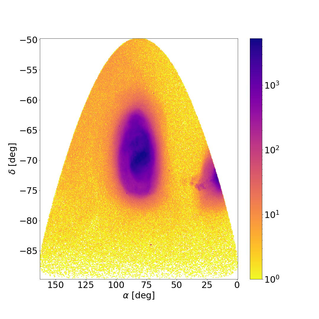
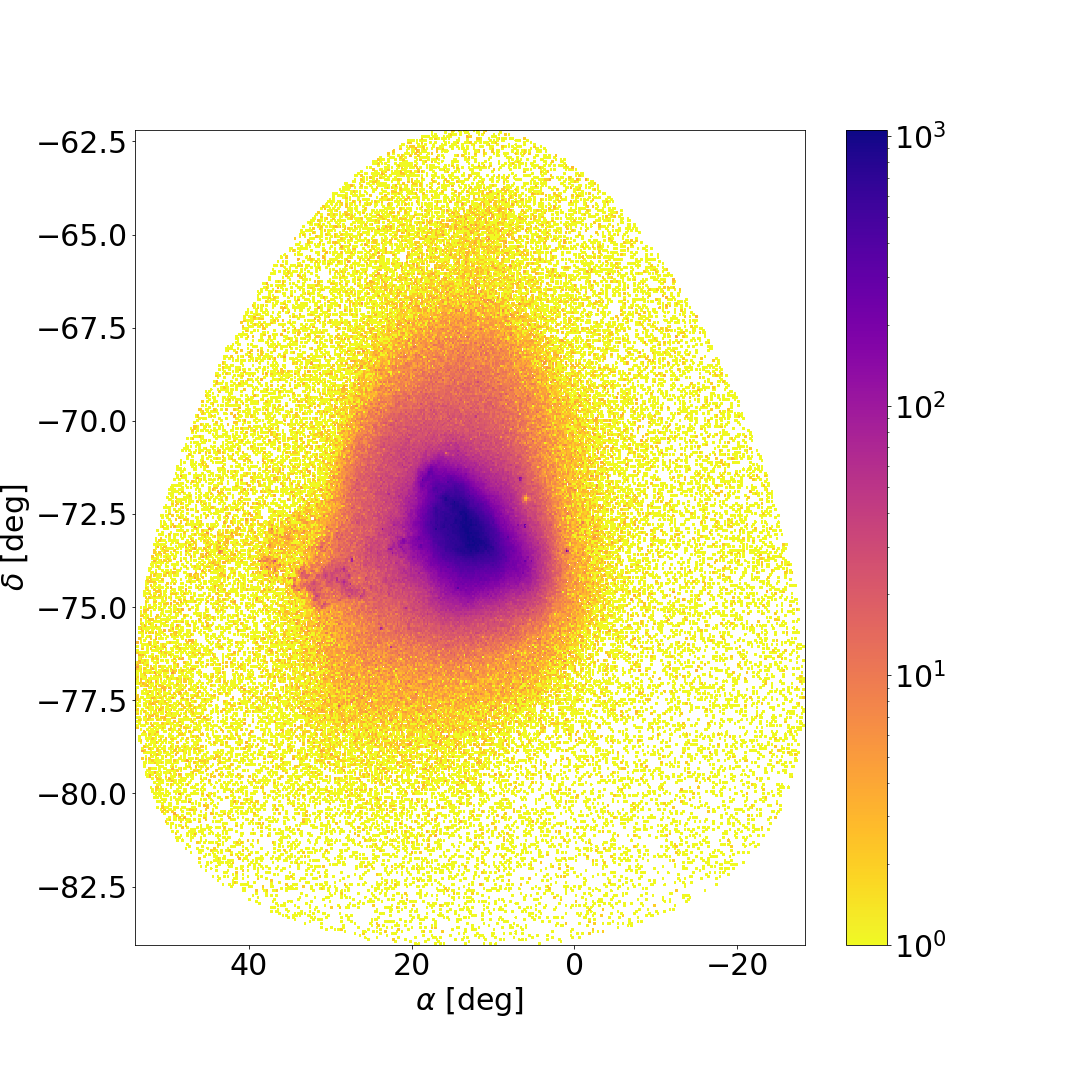
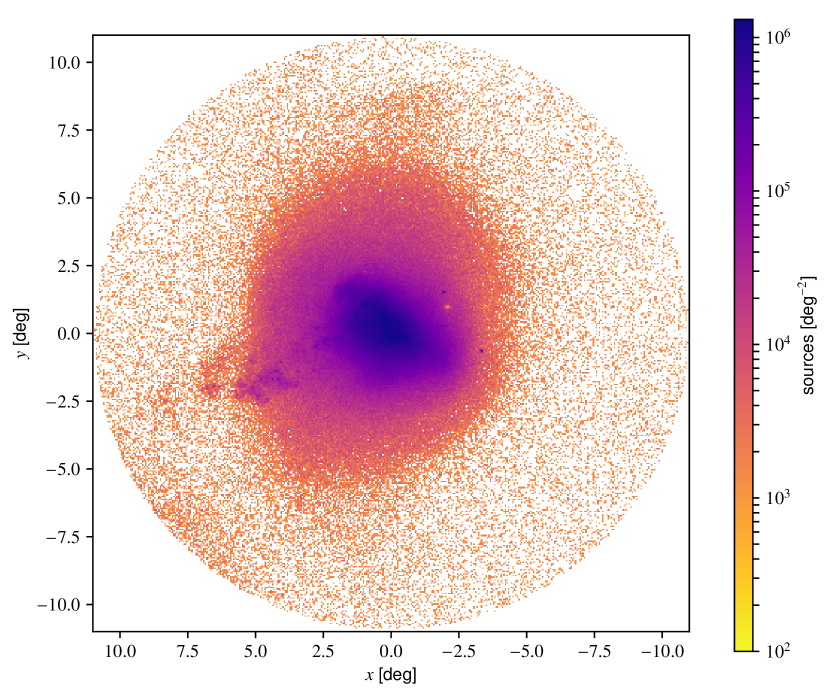
Figure 1: Sky density plots for the LMC (left) and SMC (right) clean samples (after spatial and proper motion selection). Top row: Plots in equatorial coordinates. Bottom row: Orthographic projection (as used in Sect. 3)

2.3 Evolutionary phase subsamples

The two samples obtained following the procedure outlined in the two previous sections constitute our basic selection of objects for the LMC and SMC, our clean samples for the stars of the clouds. These were used for analysis of the LMC and SMC as a whole. A selection of basic statistics and maps using these samples ispresented in Appendix A.

Several cases required a definition of subsamples that were adequate for the study of different substructures of the clouds (disc, halo, etc.), however. Ideally, we would like to select these subsamples by age, but this would require either generating our own age estimates or a cross-match with external catalogues, which is beyond the scope of a Gaia  EDR3 demonstration paper such as this. Instead, we used a different approach, using a selection of samples based on the CMD of the clouds. We defined cut-outs in the shape of polygonal regions in the $(G,G_{BP}-G_{RP})$ diagram to select the following target evolutionary phases:

Young 1:

very young main sequence (ages $<50$ Myr)

Young 2:

young main sequence ($\leavevmode\nobreak\ 50<$ age $<\leavevmode\nobreak\ 400$ Myr)

Young 3:

intermediate-age main-sequence population (mixed ages reaching up $1-2$ Gyr)

RGB:

red giant branch

AGB:

asymptotic giant branch (including long-period variables)

RRL:

RR-Lyrae region of the diagram

BL:

blue loop (including classical Cepheids)

RC:

red clump

The defined areas are shown in Fig. 2. There are unassigned areas in the CMD diagrams: this is on purpose because these unassigned areas are too mixed, affected by blended stars, or too contaminated by foreground (Milky Way) stars. The areas are exclusive, that is, they do not overlap.

This rather raw selection is not even corrected for reddening, but to some extent, it can be used as an age-selected proxy. Based on a simulation using a constant star formation rate, the age-metallicity relation by Harris & Zaritsky (2009), and PARSEC1.2 models, the estimated age distribution of the resulting subsamples is shown in Fig. 3. The figure shows that the resulting subsamples indeed have different age distributions that suffice for the purposes of this demonstration paper. For the sake of brevity, we refer to these subsamples as “evolutionary phases”.

2.3.1 LMC evolutionary phases

The polygons in the CMD diagram defining the LMC subsamples are as follows, and they are represented in Fig. 2 (left panel):

Young 1:

[0.18, 16.0], [-0.3, 10.0], [-1.0, 10.0], [-1.0, 16.0], [0.18, 16.0]

Young 2: [-1.0, 16.0

, [0.18, 16.0], [0.34, 18.0], [-1.0, 18.0], [-1.0, 16.0]

Young 3:

[-0.40, 20.5], [-0.6, 19.0], [-0.6, 18.0], [0.34, 18.0], [0.40, 18.9], [0.45, 19.5], [0.70, 20.5], [-0.40, 20.5]

RGB:

[0.80, 20.5], [0.90, 19.5], [1.60, 19.8], [1.60, 19.0], [1.05, 18.41], [1.30, 16.56], [1.60, 15.3], [2.40, 15.97], [1.95, 17.75], [1.85, 19.0], [2.00, 20.5], [0.80, 20.5]

AGB:

[1.6, 15.3], [1.92, 13.9], [3.5, 15.0], [3.5, 16.9], [1.6, 15.3]

RRL:

[0.45, 19.5], [0.40, 18.9], [0.90, 18.9], [0.90, 19.5], [0.45, 19.5]

BL:

[0.90, 18.25], [0.1, 15.00], [-0.30, 10.0], [2.85, 10.0], [1.30, 16.56], [1.05, 18.41], [0.90, 18.25]

RC:

[0.90, 19.5], [0.90, 18.25], [1.60, 19.0], [1.60, 19.8], [0.90, 19.5]

The number of objects per subsample is listed in Table 2. The sky distribution of the stars in the samples is shown in Fig. 27.

Total objects LMC	11,156,431
Young 1	23,869
Young 2	233,216
Young 3	3,514,579
RGB	2,642,458
AGB	34,076
RRL	221,100
BL	261,929
RC	3,730,351

Table 2: Object counts of LMC evolutionary phases

2.3.2 SMC evolutionary phases

The polygons in the CMD diagram defining the SMC subsamples are as follows, and they are represented in Fig. 2 (right panel):

Young 1:

[-1.00, 16.50], [-1.00, 10.00], [-0.30, 10.00], [-0.15, 15.25], [ 0.00, 16.50], [-1.00, 16.50]

Young 2:

[-1.00, 18.50], [-1.00, 16.50], [ 0.00, 16.50], [ 0.24, 18.50], [-1.00, 18.50]

Young 3:

[-0.50, 20.50], [-0.65, 20.00], [-0.65, 18.50], [ 0.24, 18.50], [ 0.312, 19.10], [ 0.312, 20.00], [ 0.50, 20.50], [-0.50, 20.50]

RGB:

[0.65, 20.50], [0.80, 20.00], [0.80, 19.50], [1.60, 19.80], [1.60, 19.60], [1.00, 18.50], [1.50, 15.843], [2.00, 16.00], [1.60, 18.50], [1.60, 20.50], [0.65, 20.50]

AGB:

[1.50, 15.843], [1.75, 14.516], [3.50, 15.00], [3.50, 16.471], [1.50, 15.843]

RRL:

[ 0.312, 20.00], [ 0.312, 19.10], [ 0.80 , 19.10], [ 0.80 , 20.00], [ 0.312, 20.00]

BL:

[0.40, 18.15], [-0.15, 15.25], [-0.3, 10.00], [2.60, 10.00], [1.00, 18.50], [0.80, 18.50], [0.40, 18.15]

RC:

[0.80, 19.50], [0.80, 18.50], [1.00, 18.50], [1.60, 19.60], [1.60, 19.80], [0.80, 19.50]

The number of objects per subsample is listed in Table 3. The sky distribution of the stars in the samples is shown in Fig. 28.

Total objects SMC	1,728,303
Young 1	7,166
Young 2	83,417
Young 3	379,234
RGB	448,948
AGB	5,887
RRL	40,421
BL	86,212
RC	634,569

Table 3: Object counts of SMC evolutionary phases

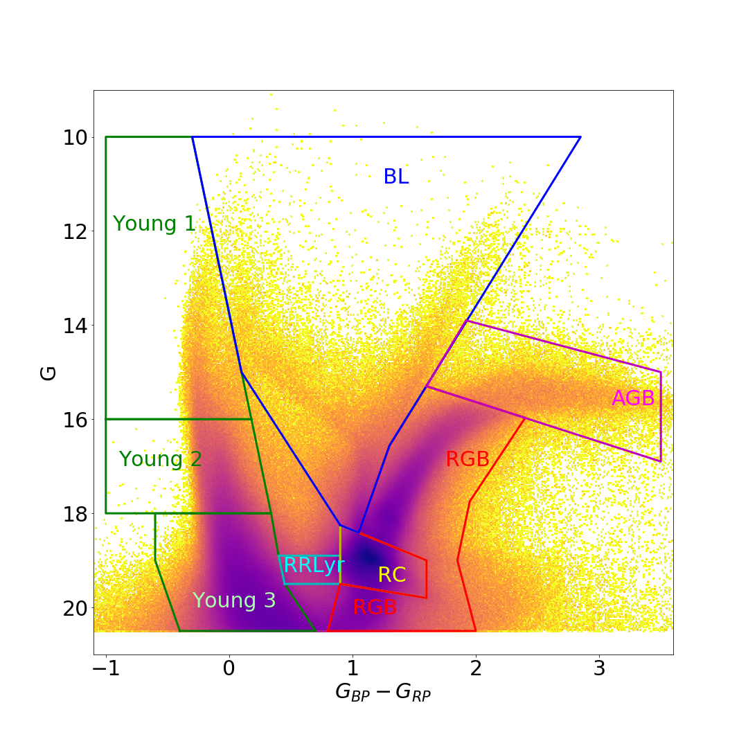
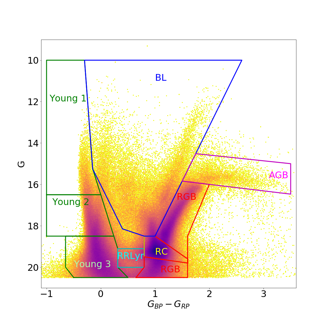
Figure 2: Areas (as defined by the polygons given in the text) of the CMD for the LMC (left) and SMC (right) evolutionary phases. The colours are not corrected for reddening for the selection.

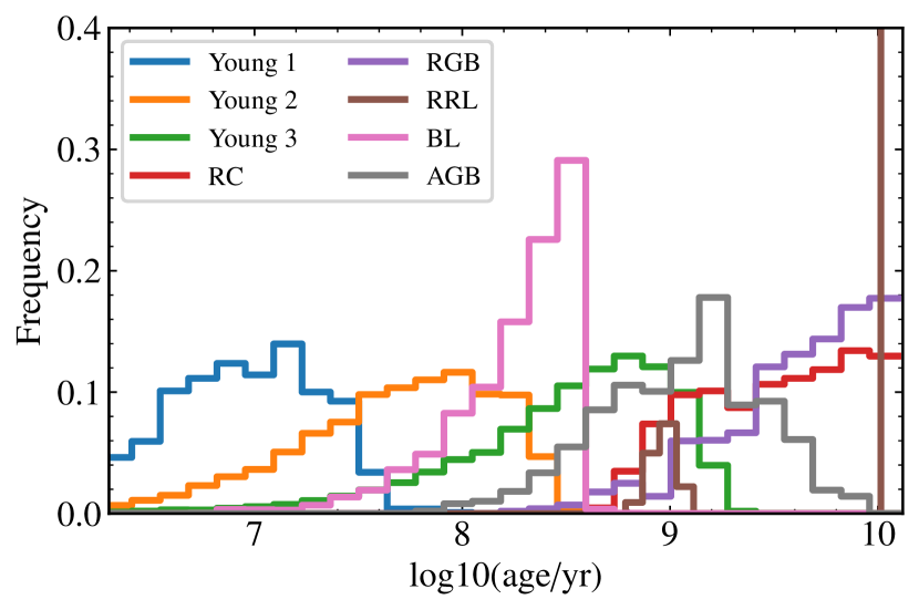
Figure 3: Estimated age distribution of the selected evolutionary phase. Based on a simulation using a constant star formation rate, the age-metallicity relation by Harris & Zaritsky (2009), and PARSEC1.2 models

3 Comparison with DR2 results

In this section we show the improvement in astrometry and photometry of sources in the Magellanic clouds in Gaia  EDR3 compared to Gaia  DR2 . The selection of sources from Gaia  DR2 for the comparison was made in the same way as for our main clean samples (as described in Sect. 2).

One of the scientific demonstration papers released with Gaia  DR2 , Gaia Collaboration et al. (2018) studied the LMC and SMC, in addition to the kinematics of globular clusters and dwarf galaxies around the Milky Way. Following this study, and to ensure that the quoted (and plotted) proper motions are relatively easy to interpret in terms of internal velocities, it is particularly helpful to define an orthographic projection of the usual celestial coordinates and proper motions,

$$\begin{aligned} x&=\cos\delta\sin(\alpha-\alpha_{C})\\ y&=\sin\delta\cos\delta_{C}-\cos\delta\sin\delta_{C}\cos(\alpha-\alpha_{C})\end{aligned},$$ (1)

where $\alpha_{C}$ and $\delta_{C}$ are the reference centres of the respective clouds (see Sect. 2.1).

The corresponding proper motions $\@vec{\mu_{xy}}=(\mu_{x},\mu_{y})$ and uncertainties in the form of a covariance matrix $\@tens{C_{\mu_{xy}}}$ can be found from $\@vec{\mu_{\alpha*\delta}}=(\mu_{\alpha*},\mu_{\delta})$, and their uncertainty covariance matrix $\@tens{C_{\mu_{\alpha*\delta}}}$ by the conversions

$$\begin{aligned} \@vec{\mu_{xy}}=&\@tens{M}\,\@vec{\mu^{T}_{\alpha*,\delta}}\\ \@tens{C_{\mu_{xy}}}=&\@tens{M}\,\@tens{C_{\mu_{\alpha*,\delta}}}\,\@tens{M}^{T}\end{aligned},$$ (2)

where

$$\@tens{M}=\begin{bmatrix}\cos(\alpha-\alpha_{C})&-\sin\delta\sin(\alpha-\alpha_{C})\\ \sin\delta_{C}\sin(\alpha-\alpha_{C})&\cos\delta\cos\delta_{C}+\sin\delta\sin\delta_{C}\cos(\alpha-\alpha_{C})\end{bmatrix}.$$ (3)

We note that at ($\alpha_{C},\delta_{C}$), we have $\mu_{x}=\mu_{\alpha*}$, $\mu_{y}=\mu_{\delta}$. We use these coordinates throughout.

In Figures 4 to 7 we show the parallax and proper motion fields of the area around each of the cloud centres, as shown in the filtered Gaia  DR2 and Gaia  EDR3 data. We use a Voronoi binning scheme (Cappellari & Copin, 2003), which produces bins with approximately 1000 stars each. The bins are therefore irregularly shaped and become large far from the centre of the clouds. Each bin is coloured according to the error-weighted mean of the indicated quantity. In each case, the dark lines are density contours.

These figures show that the Gaia  EDR3 data are a clear improvement to Gaia  DR2 data: the sawtooth variation that was seen in parallax and proper motion is significantly reduced. The outer bins of both the LMC and SMC still show a net positive parallax, which indicates that for these bins, foreground contamination that passes our proper motion and parallax filter makes a small but non-negligible contribution.

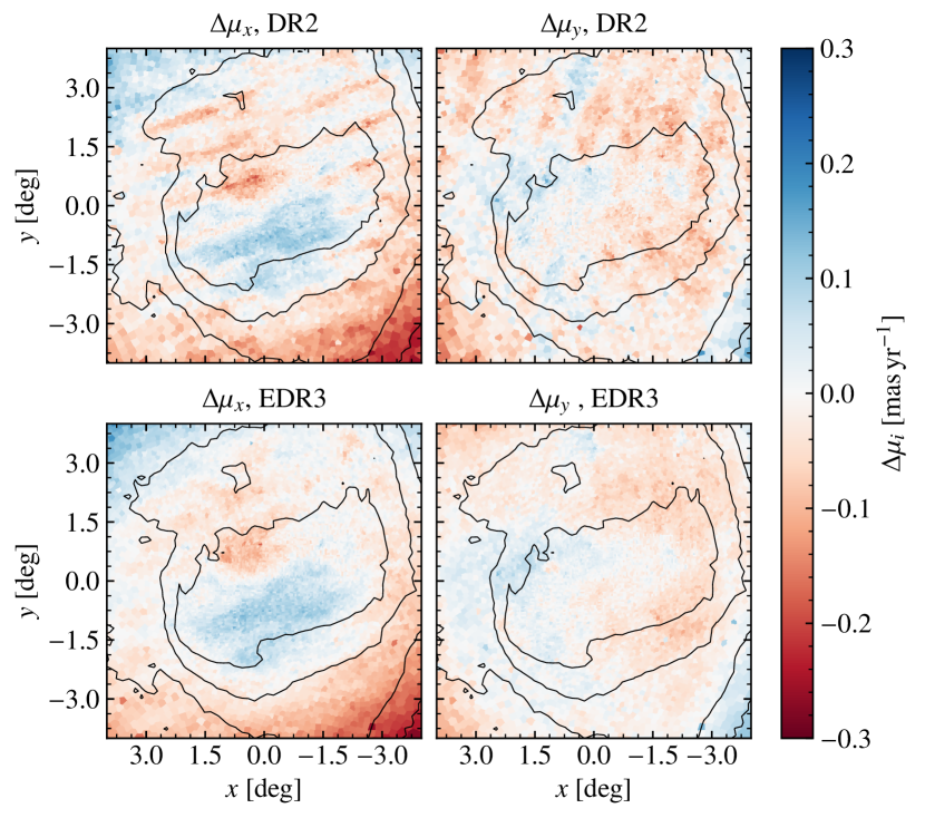
Figure 6: Comparison of the residual proper motion fields of the LMC after a first-order approximation of the field was subtracted to emphasise the systematic errors in Gaia  DR2 (upper panels) and Gaia  EDR3 (lower panels).

In Figures 6 and 7 we show the proper motions that remain when we subtracted a linear gradient from each, so we show in each case

$$\Delta\mu_{i}=\mu_{i}-\left(\mu_{i,0}+\left.\frac{\partial\mu_{i}}{\partial x}\right|_{0}x+\left.\frac{\partial\mu_{i}}{\partial y}\right|_{0}y\right),$$ (4)

where the central values, $\mu_{i,0}$, and partial derivatives ${\partial\mu_{i}}/{\partial x}$ and ${\partial\mu_{i}}/{\partial y}$ were evaluated as a linear fit to the values within a radius of $3^{\circ}$ around the centre. The values found using Gaia  EDR3 are shown in Table 4. This allows us to show the sawtooth pattern in proper motions more clearly. The patterns are again significantly reduced in Gaia  EDR3. The faint indications of a streaming motion along the bar that were pointed out in Gaia  DR2 stand out much more clearly in Gaia  EDR3, and we investigate them further in Section 7.

	$\mu_{x}$	$\mu_{y}$	$\frac{\partial\mu_{x}}{\partial x}$	$\frac{\partial\mu_{x}}{\partial y}$	$\frac{\partial\mu_{y}}{\partial x}$	$\frac{\partial\mu_{y}}{\partial y}$
LMC	1.871	0.391	-1.561	-4.136	4.481	-0.217
SMC	0.686	-1.237	1.899	0.288	-1.488	0.213

Table 4: Linear fit to the proper motions in the $x,y$ directions using Gaia  EDR3. Proper motions are in $\mathrm{mas}\,\mathrm{yr}^{-1}$, and $x,y$ positions in radians.

As explained in Gaia Collaboration et al. (2018, eq. 3), we can use the simple linear gradients to estimate the inclination, orientation and angular velocity of the disc under the assumptions that this angular velocity $\omega$ is constant, which is valid for a linearly rising rotation curve, and that the average motion is purely azimuthal in a flat disc. We define the inclination $i$ to be the angle between the line-of-sight direction to the cloud centre and the rotation axis of the disc, and orientation $\Omega$ is the position angle of the receding node, measured from $\@vec{y}$ towards $\@vec{x}$, that is, from north towards east. Here and elsewhere, we assume that the distances to the LMC and SMC are $D_{LMC}=49.5\,{\rm kpc}$ (Pietrzyński et al., 2019) and $D_{SMC}=62.8\,{\rm kpc}$ (Cioni et al., 2000b), respectively.

The line-of-sight velocity of the disc can either be derived from these gradients, or (as we do here) assumed given the known line-of-sight velocity of the LMC (van der Marel et al., 2002, $262.2\pm 3.4\,\rm{km}\,\rm{s}^{-1}$) or SMC (Harris & Zaritsky, 2006, $145.6\pm 0.6\,\rm{km}\,\rm{s}^{-1}$). The values we find for $i$, $\Omega,$ and $\omega$ are $34.538^{\circ},298.121^{\circ},4.732\;\mathrm{mas}\,\mathrm{yr}^{-1}$ and $78.763^{\circ},8.955^{\circ},0.854\;\mathrm{mas}\,\mathrm{yr}^{-1}$ for the LMC and SMC, respectively. This is broadly consistent with the values found for Gaia  DR2 . The LMC values are consistent with those found by the more detailed investigation in Sect. 5.

In Fig. 8 we use the technique of line-integral convolution (Cabral & Leedom, 1993) to better illustrate the proper motion field of the Magellanic Clouds. The direction of the lines illustrates the vector field of the proper motions, while their brightness illustrates the density (more precisely, we set the alpha parameter in matplotlib to be proportional to the $1/4$ power of the star count). The ordered rotation of the LMC is very clear from this image, while the SMC is more jumbled.

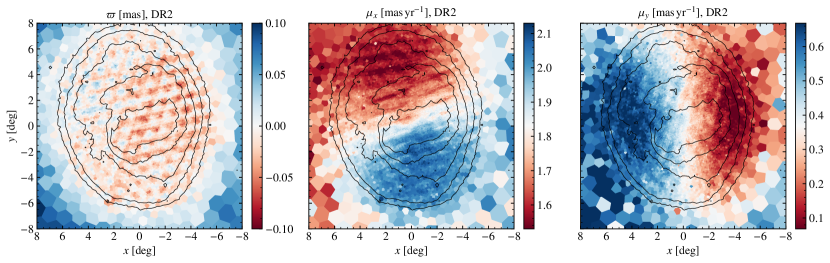
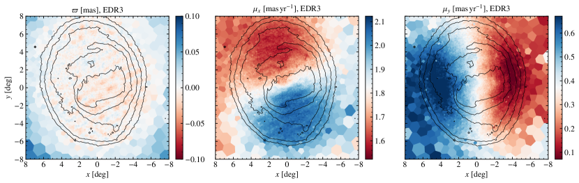
Figure 4: Comparison of the parallaxes (left) and proper motions in the $x$ and $y$ directions (middle and right, respectively) of LMC sources in Gaia  DR2 (upper panels) and Gaia  EDR3 (lower panels).

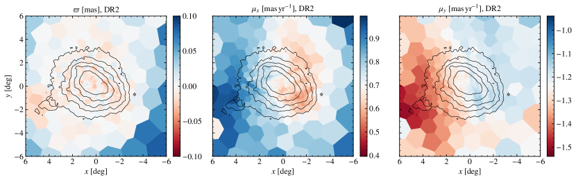
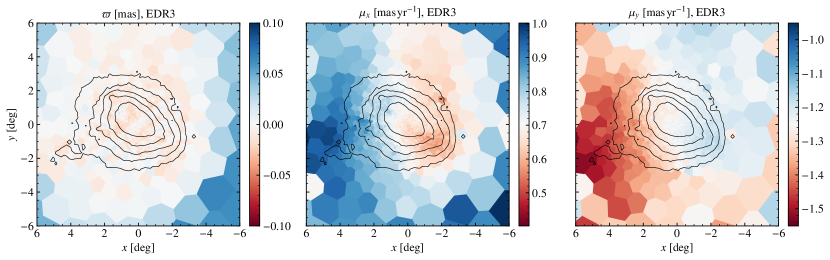
Figure 5: Same as in Fig. 4, but for the SMC.

Finally, to complete this section, we compare the quality of the photometry in the LMC and SMC areas. Extracting $G_{\rm BP}$ and $G_{\rm RP}$ photometry from prism spectra is challenging in the dense, central parts of the Magellanic Clouds. A simple diagnostic for the consistency of the photometry for a source is the photometric excess factor (included in the archive), which is defined as the ratio of the flux of the prism spectra ($G_{\rm BP}$ and $G_{\rm RP}$) and the $G$ flux. Because the two spectra overlap slightly and have a higher response in the red, this ratio typically lies in the range 1.1–1.4 for isolated point sources, with higher values for the redder sources. Fig. 24 shows that the centres of the clouds are not very red, and Fig. 9 shows that the mean excess factor increases in these centres, but with abnormally high values in Gaia  DR2 (left panel) and typical values in Gaia  EDR3 (right panel). In Gaia  EDR3 the background estimation has changed significantly as compared to Gaia  DR2 (Gaia collaboration, Riello et al., 2020), while crowding is still left uncorrected for. We conclude that the photometry in Gaia  DR2  was strongly affected by background issues in the central areas, and that this problem has greatly diminished in Gaia  EDR3, where traces of crowding are still visible. The $G$ flux has only changed slightly between the two releases, that is, by a few hundredths of a magnitude, while $G_{\rm BP}$ and $G_{\rm RP}$ have been revised by a few tenths of a magnitude. It is therefore a fair assumption that the improved excess factor is driven by the improvement of $G_{\rm BP}$ and $G_{\rm RP}$ photometry in Gaia  EDR3.

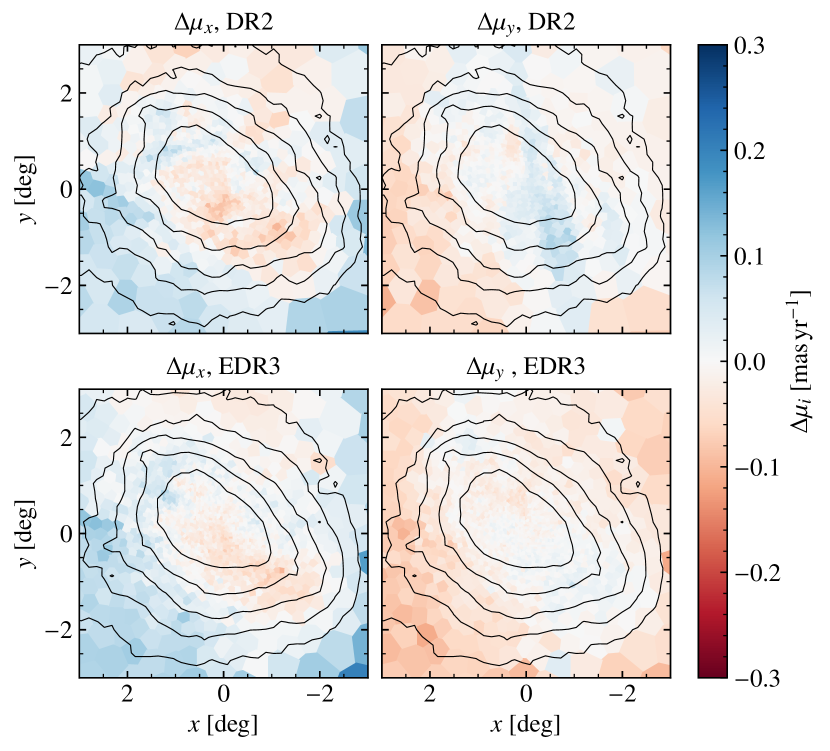
Figure 7: Same as in Fig. 6, but for the SMC.

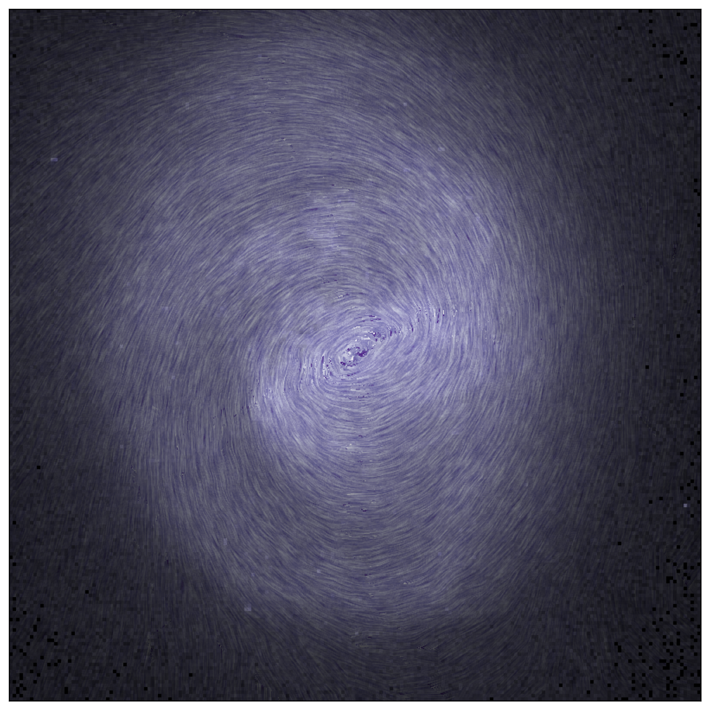
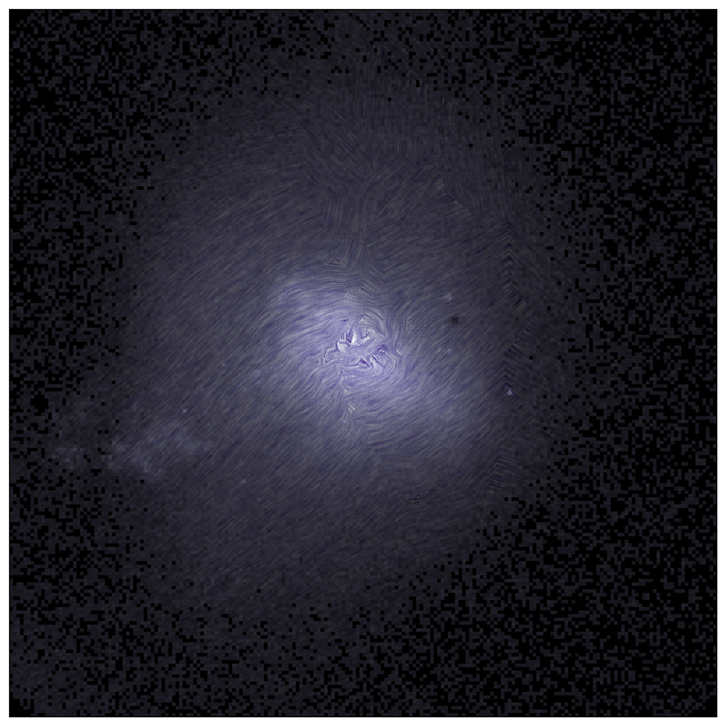
Figure 8: Illustration of the proper motion field of the LMC (left) and SMC (right) using line-integral convolution. We set the alpha parameter (opacity) of the coloured lines according to the density, with the densest regions being the most opaque.

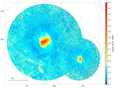
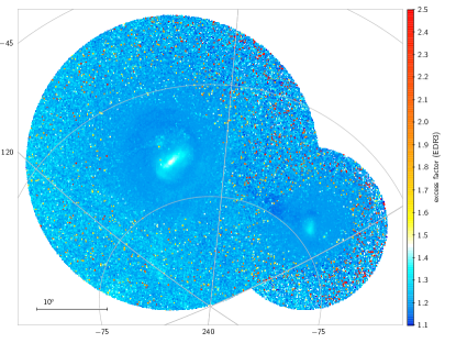
Figure 9: Photometric excess factor, i.e. the sum of fluxes in the $G_{\rm BP}$ and $G_{\rm RP}$ bands over the $G$ flux. Left: for Gaia  DR2 , and right: for Gaia  EDR3.

4 Spatial structure of the Large Magellanic Cloud

In this section we summarise our attempts to infer the spatial distribution of sources in the LMC using a simplified model without separating the various stellar populations that constitute the galaxy. This is an oversimplification (see e.g. El Youssoufi et al., 2019, for a recent summary of the complexity of the problem when the different populations are taken into account), aimed only at exemplifying the use of the Gaia astrometry for this type of studies.

Despite the significant improvement of the Gaia  EDR3 astrometry with respect to Gaia  DR2 , systematic problems remain, as described in Gaia collaboration, Lindegren et al. (2020a) and exemplified in the spatial distribution of median parallaxes shown in Fig. 4. In order to infer the parameters of the LMC spatial distribution, we therefore modelled the observed parallaxes as affected by a zero-point offset.

We assumed, for the sake of illustrating the magnitude of these zero-point offsets, that the sources selected as candidate members of the LMC have a mean parallax of 0.02 mas, corresponding to a distance of 50 kpc from the Sun (Pietrzyński et al., 2019). The central 90% interval around the median (binned) Gaia  EDR3 parallaxes shown in Fig. 4 extends from -0.075 to 0.05 mas. We can therefore estimate the range of zero-point offsets as (-0.095,0.03). This means that the zero-point offsets are of the same order of magnitude, but larger than the expected value of the mean parallax of the LMC. Variations in parallaxes around the mean value due to the spatial distribution of the LMC sources (e.g. due to its depth or inclination angle) are expected to be much smaller. In addition, these systematics occur in combination with the usual random uncertainties associated with the individual measurements that propagate to yield the catalogue parallax uncertainty of each source. In the case of the data set used here, these parallax uncertainties have a median value of 0.17 mas. Estimating the zero-point offsets therefore is a critical element of the modelling effort we describe in this section and plays a central role in the inference of the parameters of the spatial structure of the LMC.

Unfortunately, we did not succeed in our aim of inferring geometric properties of the LMC from the Gaia  EDR3 astrometric measurements. We tried several degrees of model complexity and two approaches to the inference problem: Markov chain Monte Carlo posterior sampling (MCMC) (Robert & Casella, 2013), and approximate Bayesian computation (ABC) (Beaumont et al., 2002; Marjoram et al., 2003), always in the context of the Bayesian approach to inference. In the MCMC posterior sampling we used the parallaxes of the individual LMC sources to compute the full likelihood, while in the ABC approach, we binned the data in a certain number of constant-size right ascension and declination bins and employed a distance metric to compare simulations and observations in order to avoid computing the full likelihood.

Both approaches used the same probabilistic generative model for the distribution of the Gaia  EDR3 parallax measurements. This model assumes that the LMC sources are spatially distributed as an elliptic double -exponential disc (similarly as in Eq. (1) of Mancini et al. (2004), but with the vertical distances from the disc mid-plane modelled by a central Laplace prior) and generates as many (proper to the disc) location coordinates as there are sources in the Gaia  EDR3 sample. The model applies a number of geometrical transformations (see e.g. Weinberg & Nikolaev 2001) to generate a set of true parallaxes that are unaffected by the measurement uncertainties and/or zero-point offsets. Our generative model has nine global parameters: the disc scale length $R_{0}$, the disc scale height $h_{0}$, the disc ellipticity parameter $\epsilon$, the disc minor-axis position angle $\theta_{\mathsf{ma}}$ , and the LMC line of nodes position angle $\theta_{\mathsf{LON}}$ (both angles measured with respect to the west direction), the inclination angle $i$ of the LMC plane with respect to the plane of the sky, and the spherical coordinates $\left(\alpha_{0},\delta_{0},D_{LMC}\right)$ of the centre of the LMC disc.

To simulate observed parallaxes, we took the Gaia  EDR3 parallax uncertainties (the variance error component) and the parallax zero-point offset patterns (the systematic error component) observed in the Gaia  EDR3 data into account. We modelled the latter as part of the inference process by means of a linear combination of Gaussian radial basis functions (RBFs) using the observed patterns and a canonical distance to the LMC as initial guess. Finally, each parallax measurement was simulated using a Gaussian distribution centred at the sum of the true simulated parallax and the offset generated using the RBF model.

In addition to modelling the parallax zero-point offsets using the RBF parametrisation as part of the inference process, we also tried to correct individual source parallaxes using an early version of the fit proposed in Gaia collaboration, Lindegren et al. (2020a) as a function of the apparent magnitude and colour. Unfortunately, the correction is not useful for our purposes. The mentioned correction (from Gaia collaboration, Lindegren et al., 2020a) is obtained by a combination of information from quasars, physical stellar pairs, and LMC sources. However, it is not able to reproduce the local variations of the parallax zero-point in the LMC field because its only dependence on positions is of the form of the sinus of the ecliptic latitude, which is almost constant in the LMC area. Additionally, the correction assumes that all the LMC stars are at the same distance embedding its internal 3D structure, which is what we aimed to determine.

In what follows we describe our attempt of using the probabilistic generative model to perform the parameter inference using the MCMC algorithm. We attempted to evaluate the full likelihood for several of the populations defined in Sect. 2. The inference process was based on a hierarchical Bayesian model and an MCMC no-U-turn posterior sampler (NUTS) (Hoffman & Gelman, 2014). In this approach the true parallax of individual LMC sources was used to compute the likelihood. This implies the inclusion of one additional parameter per source (its true distance). The computational demands were so high that we were forced to distribute the likelihood computations in a TensorFlow (Abadi et al., 2016) Probability (Dillon et al., 2017) framework in the Mare Nostrum supercomputer at the Barcelona Supercomputing Centre. Unfortunately, the maturity level of the TensorFlow libraries involved was not sufficient and we did not achieve the required performance accelerations. Then, our main problem was that we were unable to scale our models to the size of the Gaia  EDR3 sample using the MCMC NUTS algorithm.

Because of the scalability issues found when using the MCMC, we decided to try with a sequential Monte Carlo approximate Bayesian computation algorithm (SMC-ABC), which is further described in Jennings & Madigan (2017) and section 5 of Mor et al. (2018). The theoretical basis for these algorithms can be found in Marin et al. (2011) , Beaumont et al. (2008), and Sisson & Fan (2010).

The choice of the summary statistics is crucial for the performance of the SMC-ABC algorithm. For the purposes of the present work, we defined the summary statistics as the median parallax of the stars in the LMC sample, distributed in a grid of 50$\times$50 bins in right ascension (from $50\deg$ to $120\deg$) and declination ($-50\deg$ to $-80\deg$). The stellar sample used for this inference was the combination of the following subsamples: Young 1, Young 2, Young 3, RGB, AGB, RRL, BL, and RC.

With the SMC-ACB technique we attempted to infer up to seven parameters of the structure of the LMC: the distance to the centre $D_{LMC}$, the inclination angle $i$, the position angle of the line of nodes $\theta_{\mathsf{LON}}$, the position angle of the disc minor axis $\theta_{\mathsf{ma}}$, the ellipticity factor $\epsilon,$ and the position in the sky of the LMC centre $\left(\alpha_{0},\delta_{0}\right)$. To infer these structural parameters, we chose Gaussian priors centred on the standard values found in the literature; the prior in distance is the most restrictive. Furthermore, we simultaneously inferred the model parameters of the parallax zero-point variations (i.e. the coefficients of the RBF linear model described above) using 50 basis functions. Additionally, we fixed the scale height and the radial scale length of the disc at $1.6$ and $0.35$ kpc, respectively.

From the SMC-ABC attempt, our conclusion is that the local parallax zero -point of the LMC in Gaia  EDR3 distorts most of the signal of the 3D structure of the LMC (in the astrometry), and that there is not enough information in our summary statistics to simultaneously infer the local parallax zero-point variations and the 3D structure of the LMC. However, it may be possible if the former is constrained with additional external restrictions and/or finding an optimal way to add the information from the density distribution of the stars in the LMC area.

5 Kinematics of the Large Magellanic Cloud

In this section we use the Gaia  EDR3 data to study the kinematics of the Magellanic Clouds. The analysis is focused on the LMC because it has a clear disc structure that can be meaningfully modelled and understood; the SMC has a more complex, irregular structure that would require a more extensive and deep analysis, which is beyond the scope of this demonstration paper.

In the Sect. 5.1 we describe the method and tools we used in our analysis, and in Sect. 5.2 we present an analysis of the general kinematic trends and a detailed look at the velocity profiles in the disc, focusing on the segregation of the rotation velocities as a function of the evolutionary stage.

5.1 Method and tools

Gaia Collaboration et al. (2018) presented formulae relating the in-plane velocities of stars to their observed proper motions under the assumption that the stars all move in a flat disc. Here we summarise the key results and equations.

Defining:

• $a=\tan i\cos\Omega$

• $b=-\tan i\sin\Omega$

• $(l_{x},l_{y})=(\sin\Omega,\cos\Omega)$

• $(m_{x},m_{y},m_{z})=(-\cos i\cos\Omega,\cos i\sin\Omega,\sin i)$

Gaia Collaboration et al. (2018) show that Cartesian coordinates can be defined in the plane of the disc $\xi,\eta,$ where

$$\begin{aligned} \xi&=\frac{l_{x}x+l_{y}y}{z+ax+by}\\[3.0pt] \eta&=\frac{(m_{x}-am_{z})x+(m_{y}-bm_{z})y}{z+ax+by}\end{aligned},$$ (5)

and derive simultaneous equations relating the velocities $\dot{\xi},\dot{\eta}$ to $\mu_{x},\mu_{y}$ for a given disc inclination, orientation, and bulk velocity of the galaxy can derived. The bulk velocity of the galaxy is expressed as $(\mu_{x,0},\mu_{y,0},\mu_{z,0})$, where $\mu_{x,0}$ and $\mu_{y,0}$ are the associated proper motions in the $x$ and $y$ directions at the centre of the disc, and $\mu_{z,0}=v_{z,0}/D_{LMC}$, the associated line-of-sight velocity, expressed on the same scale as the proper motions by dividing by $D_{LMC}$. We derive

$$(l_{x}- x(l_{x}x+l_{y}y))\dot{\xi}+(m_{x}-x(m_{x}x+m_{y}y+m_{z}z))\dot{\eta}$$ (6)

$$=-\mu_{x,0}+x(\mu_{x,0}x+\mu_{y,0}y+\mu_{z,0}z)+\frac{\mu_{x}}{ax+by+\sqrt{1-x^{2}-y^{2}}}$$

$$(l_{y}- y(l_{x}x+l_{y}y))\dot{\xi}+(m_{y}-y(m_{x}x+m_{y}y+m_{z}z))\dot{\eta}$$

$$=-v_{y}+y(\mu_{x,0}x+\mu_{y,0}y+\mu_{z,0}z)+\frac{\mu_{y}}{ax+by+\sqrt{1-x^{2}-y^{2}}}.$$

Furthermore, we can gain much more physical insight by converting these Cartesian coordinates $\xi,\eta,\dot{\xi},and\dot{\eta}$ into polar coordinates $R,\phi,v_{R},\text{and }v_{\phi}$.

Our strategy in this paper therefore was to fit the proper motion of the filtered LMC population as a flat rotating disc with average $v_{R}=0$ and $v_{\phi}=v_{\phi}(R)$. Our model has ten parameters, some of which can be kept fixed (based on the other knowledge of the Magellanic Clouds):

• Rotational centre of the disc on sky, parametrised as $(\alpha_{0},\delta_{0})$

• Bulk velocity in the $x$ direction, which we parametrise as $\mu_{x,0}$, the associated proper motion at the centre of the disc.

• Bulk velocity in the $y$ direction, which we parametrise as $\mu_{y,0}$, the associated proper motion at the centre of the disc.

• Bulk velocity in the $z$ direction, which we parametrise as $\mu_{z,0}=v_{z,0}/D_{LMC}$.

• Inclination, $i$.

• Orientation, $\Omega$.

• Three parameters ($v_{0}$, $r_{0}$ and $\alpha$) are used to describe the rotation curve,

  $$v_{\phi,M}(R)=v_{0}\left(1+\left({r_{0}\over R}\right)^{\alpha}\right)^{-1/\alpha}$$

To analyse the data, we considered bins of $0.08^{\circ}$ by $0.08^{\circ}$ in $x,y$ in the range $-8^{\circ}<x<8^{\circ}$, $-8^{\circ}<y<8^{\circ}$. For each bin with centre $x_{i},y_{i}$, we derived a maximum likelihood estimate of the typical proper motion, that is, for the $i$th bin, $\@vec{\mu_{i}}=(\mu_{x,i},\mu_{y,i}$), and dispersion matrix

$$\@tens{\Sigma}_{i}=\begin{bmatrix}\sigma_{x,i}^{2}&\rho_{\sigma xy,i}\sigma_{x,i}\sigma_{y,i}\\ \rho_{\sigma xy,i}\sigma_{x,i}\sigma_{y,i}&\sigma_{y,i}^{2}\end{bmatrix}$$ (7)

by maximising

$$\begin{aligned} \mathcal{L}_{i}=\prod_{j=1}^{N_{i}}&\frac{1}{2\pi\sqrt{|\@tens{\Sigma}+\@tens{C}_{\mu_{xy},j}|}}\\ &\;\times\exp\left(-\frac{1}{2}(\@vec{\mu}_{j}-\@vec{\mu_{i}})^{T}(\@tens{\Sigma}_{i}+\@tens{C}_{\mu_{xy},j})^{-1}(\@vec{\mu}_{j}-\@vec{\mu_{i}})\right)\end{aligned},$$ (8)

where the product is over all $N_{i}$ sources in our sample in the $i$th bin, $\@vec{\mu}_{j}$ is the quoted proper motion of the source $(\mu_{x,j},\mu_{y,j})$, and $\@tens{C_{\mu_{xy},j}}$ is the covariance matrix associated with the uncertainties as derived in Section 3.

We estimated the uncertainty of $\@vec{\mu_{i}}$ by bootstrap resampling within each pixel. This gave us an estimate of the error covariance matrix in proper motion for the bin, $\@tens{C_{\mu_{xy},i}}$. As a simple way of taking systematic errors in proper motion into account, we added a systematic uncertainty of 0.01 $\mathrm{mas}\,\mathrm{yr}^{-1}$ for each component of proper motion, isotropically. This is smaller than the statistical uncertainty in most bins outside the inner $\sim$$3^{\circ}$. We chose this value because it is of the same order as the spatially dependent systematic errors found by Gaia collaboration, Lindegren et al. (2020a). Binning the data allowed us to make this correction for systematic uncertainty and reduced the computational difficulty of fitting the model.

The parameters $\mu_{x,0},\mu_{y,0},\mu_{z,0},i,$ and $\Omega$ give a conversion between the $(x_{i},y_{i},\mu_{x,i},\mu_{y,i})$ values for each pixel and the corresponding positions and velocities in the frame of the LMC, $(R_{i},\phi_{i},v_{R,i},\text{and }v_{\phi,i})$ thorugh Eq. (6). We also converted the corresponding uncertainty matrix in proper motion into one for $v_{R,i},v_{\phi,i}$ (for these values of $\mu_{x,0},\mu_{y,0},\mu_{z,0},i,$ and $\Omega$), which we refer to as $\@tens{C_{(v_{R},v_{\phi}),i}}$. The statistic that we then calculate is chi-square-like,

$$\chi^{2}=\sum_{i=1}^{N_{bins}}\@vec{(\Delta v_{i})}^{T}\@tens{C_{(v_{R},v_{\phi}),i}}\@vec{(\Delta v_{i})}$$ (9)

with $\@vec{(\Delta v_{i})}=\left(v_{R,i},v_{\phi,i}-v_{\phi,M}(R_{i})\right)$.

We note that the statistical uncertainties on the values we quote are very small. They are $\sim$$0.2\,\mu\mathrm{as}\,\mathrm{yr}^{-1}$ on $\mu_{x,0}$ and $\mu_{y,0}$, and less than $0.5$ % on the derived quantities such as $\mu_{z,0}$ or $i$. We emphasise therefore that systematic errors, particularly those due to our simple model, are the dominant uncertainty. The difference between values in table 5 can be seen as a gauge of these systematic errors.

Our main analysis takes the centre of rotation $(\alpha_{0},\delta_{0})$ as fixed at the photometric centre $\alpha_{C},\delta_{C}$ (Sect. 2), and $\mu_{z,0}=1.115\mathrm{mas}\,\mathrm{yr}^{-1}$ taking the value from spectroscopy (Sect. 3). The parameters of this model, found by minimising $\chi^{2}$, are given in Table 5 (along with those from the other models we considered).

Model	$\alpha_{0}$	$\delta_{0}$	$\mu_{x,0}$	$\mu_{y,0}$	$\mu_{z,0}$	$i$	$\Omega$	$v_{0}$	$r_{0}$	$\alpha_{RC}$
	(deg)	(deg)	($\mathrm{mas}\,\mathrm{yr}^{-1}$)	($\mathrm{mas}\,\mathrm{yr}^{-1}$)	($\mathrm{mas}\,\mathrm{yr}^{-1}$)	(deg)	(deg)	(km s-1)	(kpc)
Main	$[81.28]$	$[-69.78]$	$1.858$	$0.385$	$[1.115]$	$34.08$	$309.92$	$75.9$	$2.94$	$5.306$
$\mu_{z,0}$ free	$[81.28]$	$[-69.78]$	$1.858$	$0.385$	$1.179$	$34.95$	$310.93$	$76.5$	$2.96$	$5.237$
Centre free	$81.07$	$-69.41$	$1.847$	$0.371$	$[1.115]$	$33.28$	$310.97$	$74.2$	$2.89$	$6.160$
Centre free, $r_{\rm min}=1^{\circ}$	$81.14$	$-69.42$	$1.847$	$0.374$	$[1.115]$	$33.21$	$311.26$	$74.0$	$2.96$	$7.110$
Centre free, $r_{\rm min}=2^{\circ}$	$81.34$	$-69.48$	$1.845$	$0.383$	$[1.115]$	$33.24$	$312.74$	$73.5$	$3.21$	$13.529$
Centre free, $r_{\rm min}=3^{\circ}$	$81.59$	$-69.55$	$1.844$	$0.394$	$[1.115]$	$33.31$	$313.35$	$72.1$	$0.20$	$4.901$

Table 5: Parameters of the kinematic model fit to our data. Values in square brackets are held fixed for that model.

We also considered the case where we did not fix $\mu_{z,0}$, but left it as a free parameter. We find a value of $1.179\mathrm{mas}\,\mathrm{yr}^{-1}$, corresponding to a line-of-sight velocity of $288$km s^-1, which is a difference of about 7 % from the value known from spectroscopy. The difference in inclination and orientation is around $1.5^{\circ}$ in each case, and the bulk motion in $x$ and $y$ is almost unchanged. The ability of measuring $\mu_{z,0}$ from the proper motions alone comes from the perspective contraction of the LMC as it moves away from the Sun, but we cannot expect this model-dependent result to provide a more accurate measure than from a spectroscopic study.

Finally, we considered the question of the rotational centre of the LMC. The easiest way to do this within our analysis is to allow the centre of the $x,y$ coordinate system to shift, and then recalculate the binned values $x_{i},y_{i},\mu_{x,i},\text{and }\mu_{y,i}$ and uncertainties in the new coordinate system (in practice, we converted the binned values into equatorial coordinates, and then converted into the new coordinate system, rather than rebinning each time). The rotational centre of the LMC has been a matter of debate, most notably with the photometric centre and the centre of rotation for the Hi gas lying at different positions. The photometric centre was found to be ($81^{\circ}.28,-69^{\circ}.78$) by van der Marel (2001), who also found that the centre of the outer isopleths (corrected for viewing angle) was at $(82^{\circ}.25,-69^{\circ}.50)$. The kinematic centre of the Hi gas disc has been found to be $(79^{\circ}.40,-69^{\circ}.03)$ by Kim et al. (1998) or $(78^{\circ}.13,-69^{\circ}.00)$ by Luks & Rohlfs (1992). Using Hubble Space Telescope (HST) proper motions in the LMC, van der Marel & Kallivayalil (2014) found a rotational centre ($78^{\circ}.76\pm 0^{\circ}.52,-69^{\circ}.19\pm 0.25^{\circ}$) that lies close to the centre of rotation for the Hi gas, but pointed out that this was inconsistent with the rotational centre derived from studies of the line-of-sight velocity distribution in carbon stars (van der Marel et al., 2002, e.g. $81^{\circ}.91\pm 0^{\circ}.98,-69^{\circ}.87\pm 0^{\circ}.41$). More recently, Wan et al. (2020) used Gaia  DR2 proper motions, along with SkyMapper photometry (Wolf et al., 2018) to find dynamic centres for carbon stars, RGB stars, and young stars – $(80^{\circ}.90\pm 0^{\circ}.29,-68^{\circ}.74\pm 0^{\circ}.12)$, $(81^{\circ}.23\pm 0^{\circ}.04,-69^{\circ}.00\pm 0^{\circ}.02),$ and $(80^{\circ}.98\pm 0^{\circ}.07,-69^{\circ}.69\pm 0^{\circ}.02),$ respectively.

We derive a centre of $(81^{\circ}.01,-69^{\circ}.38)$ when this was left as a free parameter, which is somewhat closer to the photometric centre than to the Hi centre. The inner regions of the galaxy do not provide much information in the proper motion field to find the centre because to first order, a linearly rising rotation curve produces a linearly varying proper motion field, so that the position of the centre is degenerate with the bulk velocity. The centre of the LMC does, however, have a significant non-circular motion, which is not captured by our model, and large statistical weight in our calculations (because of the high density of stars). We therefore investigated whether cutting data from the inner few degrees of the LMC changed our results. We did this by cutting data from our analysis with $x^{2}+y^{2}<r^{2}_{\rm min}$ (taking $x$ and $y$ from our original coordinate system, so that the data were the same for any centre considered), and re-deriving the parameters. The results are again listed in Table 5. The rotational centre moves slightly closer to the photometric centre as we cut larger areas from the centre of our dataset, suggesting that this result is robust against some of the incompleteness of our kinematic model. We tested whether changing the centre of our cut region affects the results (e.g. cutting data centred on the rotational centre of the Hi gas instead), and the differences are very small.

In Figure 10 we show the different proposed centres of rotation on a stellar density map of the centre of the LMC. The centres derived from Gaia  EDR3 are closer to those from photometric studies than to those from the rotation of H i gas or from proper motions measured by the HST. The change in centre also naturally produces a change in derived bulk velocity, inclination, and orientation of the disc. The bulk velocity changes by $\sim$$0.02\,\mathrm{mas}\,\mathrm{yr}^{-1}$, which at the distance of the LMC corresponds to a velocity difference of $5$km s^-1. The inclination and orientation only change by about $1^{\circ}$. We show plots of $v_{\phi}$ and $v_{R}$ for our main model, and our model with the centre left as a free parameter (considering all data), in Fig. 11. As expected, the differences are relatively minor, although the outer parts the north-south asymmetry of the $v_{\phi}$ field is clearly reduced when the centre is left as a free parameter. The strong east-west asymmetry in $v_{R}$ near the centre is also reduced (but because the minimum in $v_{\phi}$ also appears to be offset from the centre, we are cautious about giving too much weight to this fact).

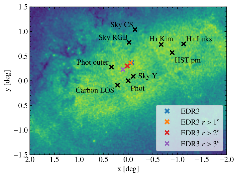
Figure 10: Positions of the centre of the LMC as found by different studies (as described in the text, SkyMapper estimates are referred to as ‘Sky’ in the figure) superimposed on an image coloured according to the total density in star counts in the inner few degrees of the LMC. The centres found in this study lie closer to the photometric centre than to the centre of H i rotation.

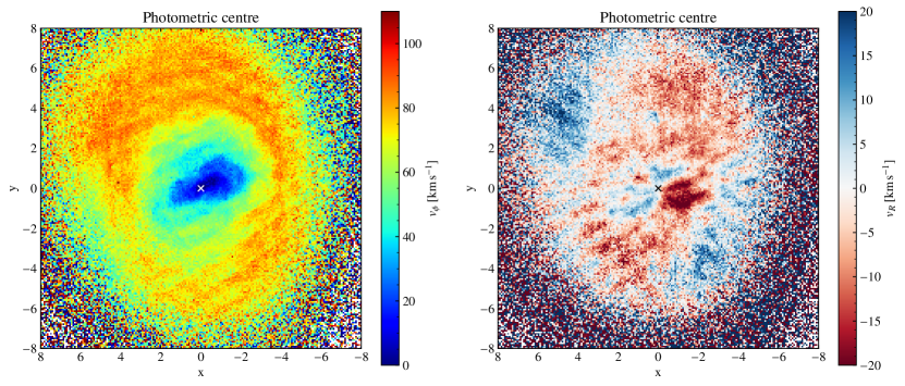
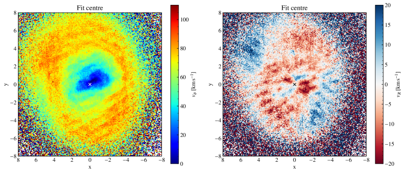
Figure 11: Plots of $v_{\phi}$ and $v_{R}$ for our main model (top) and for our model with the centre left as a free parameter (bottom).

5.2 Kinematics analysis

After we robustly constrained the main parameters with the simple rotation model, we built maps of the azimuthal and radial velocities and velocity dispersions for each of the stellar evolutionary phases of the LMC, as well as for a sample combining all phases. This latter sample is referred to as the combined sample in this section and in Sect. 7. These maps were thus derived at fixed and constant parameters with radius, as given by the main model of Sect. 5.1 ($i=34\degr$, $\Omega=310\degr$, $\alpha_{0}=81.28\degr$, $\delta_{0}=-69.78\degr$, $\mu_{x,0}=1.858\,\rm mas\,yr^{-1}$, $\mu_{y,0}=0.385\,\rm mas\,yr^{-1}$ , and $\mu_{z,0}=1.104\,\rm mas\,yr^{-1}$).

The angular resolution of the maps can be chosen to be as high as possible. In practice, the maps were made of $400\times 400$ squared pixels of 0.04° size, which is sufficiently resolved for the simple analysis of the kinematics proposed here, and it avoids more significant statistical noise inherent to higher resolutions. At the assumed distance to the LMC, it corresponds to a linear scale of 35 pc, which is equivalent to that of observations made at 0.7″  resolution (i.e. the typical seeing at e.g. the ESO Very Large Telescope) of galaxies located at the periphery of the local 10 Mpc volume. At this resolution, the maximum number of stars per pixel is 599, 288, 265, 239, 136, 105, 54, 52, and 13 for the combined, Young 3, RC, RGB, Young 2, BL, RRL, Young 1, and AGB samples, respectively. Despite the low surface density of the AGB, we were able to infer useful quantities, and we found that on average, AGB star kinematics compare well with other evolutionary phases. The maximum likelihood of Eq. (8) then yields the tangential and radial components of the velocity and velocity dispersion for each pixel.

5.2.1 General trends

Appendix B presents the $v_{\phi}$, $v_{R}$, $\sigma_{\phi}$ , and $\sigma_{R}$  maps for the eight stellar LMC subsamples, as well as those of the combined sample. These maps are the first of their kind ever obtained for an extragalactic disc, and the first maps that cover the integrality of the stellar kinematics for a galactic disc. To keep the description short in view of such a large quantity of kinematic data for a single galaxy, we present here example maps for two evolutionary phases only. We selected an evolved phase (RC stars) and a less evolved phase (Young 2 stars), which are both assumed to trace the kinematics of older and younger stellar ages.

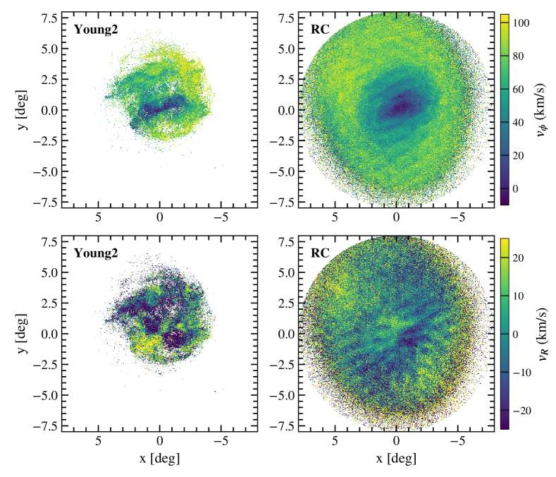
Figure 12: Example of velocity maps for the LMC. The left and right columns show young and evolved evolutionary phases (Young 2 and RC, respectively, see Sect. 2.3). The upper and bottom rows show $v_{\phi}$ and $v_{R}$, respectively. The linear velocity scales shown by colour bars are the same for the two stellar evolutionary phases and were chosen to show the structure inside the velocity fields more clearly.

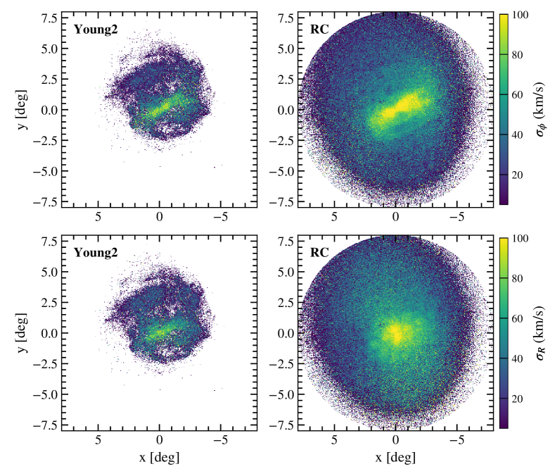
Figure 13: Same as in Fig. 12, but for the velocity dispersion.

The $v_{\phi}$ and $v_{R}$ maps of the two phases are shown in Fig. 12 and their corresponding velocity dispersion maps in Fig. 13. They all exhibit the noisy sawtooth patterns visible in the Gaia proper motion fields (Sect. 3), as well as variations occurring at larger angular scales that may likely reflect the perturbed kinematics in the spiral arms and the bar (see also Sect. 7).

Such maps present the diversity and similarity in kinematics of the various stellar evolutionary phases. For instance, the younger phase presents higher tangential motions than the older phase (e.g. 45 versus 27 km s^-1 at $R=1$ kpc, or 88 versus 77 km s^-1 at $R=4$ kpc, on average), which is a beautiful signature of the asymmetric drift, while both of them present lower velocities in a region that is apparently aligned with the stellar bar, with tens of pixels sometimes at negative values (e.g. down to $\sim-25$ km s^-1). It needs to be investigated further whether these negative values reveal counter-rotation in the bar or artificial features resulting from incorrect assumptions in this perturbed region of the disc, that is, that the stars only orbit in the $z=0$ mid-plane and with $v_{z}=0$.

The radial velocity map shows similar trends, with stronger motions for the young phase than for the RC sample. Overall, the radial motion is mostly negative for $R\lesssim 5$ kpc, indicating inwards bulk motions towards the centre of the LMC, although this picture strongly depends on the location in the disc. Alternating negative and positive velocity patterns as a function of the azimuthal position, apparently centred on the assumed photocentre at $x=y=0$, are indeed visible in the bar and spiral arms. Similarly to the rotation velocity, the velocity streaming of $v_{R}$ appears to be weaker for the older stars than for the less evolved stars.

The radial and tangential velocity dispersion maps are also rich in information. Globally, the radial dispersion dominates the tangential dispersion in both samples, and the difference between the components increases with radius. There is an extended pattern of large random motions aligned with the bar in both kinematic tracers, but also a dominant feature in $\sigma_{R}$ that is perpendicular to the bar (only for the RC sample). In this inner region of the bar, $\sigma_{R}$ is also observed to be larger where $\sigma_{\phi}$ is lower for RC stars, which indicates a variation in the velocity anisotropy as a function of the azimuthal position in the bar region. As for the comparison of the samples, random motions of the RC sample are always larger than those for the young stars (e.g. 105 versus 80 km s^-1 in the innermost pixels, or 45 versus 20 km s^-1 at $R=3$ kpc, on average), as expected for more evolved stars that lie in a thicker disc component than younger stars.

5.2.2 Velocity profiles

The 36 velocity profiles are shown in Appendix B. The profiles are the median values of all pixels from the maps located in radial bins of 200 pc width. This angular sampling suffices to identify variations of slope and amplitude in curves in the evolutionary phases. Radial bins with fewer than 5 pixels were discarded. The associated errors were derived from bootstrap resamplings of the velocity distributions and velocity dispersion at a given radial bin, at the 16th and 84th percentiles.

Figure 14 summarises the segregation of $v_{\phi}$ as a function of the evolutionary stage. The more evolved the stellar population, the shallower the rotation curve at low radius, and the lower the amplitude; this is an expected result from the asymmetric drift. Taking Young 1 as a reference sample with the highest values, we find that on average, the amplitude of the rotation curve of Young 2 stars is smaller by 0.6 km s^-1  (thus similar within the errors), and that of the BL, Young 3, AGB, RGB, RC, and RRL samples by 6, 10, 13, 17, 18, and 22 km s^-1 , respectively. The amplitude of the combined sample lags by 15 km s^-1, as it is indeed dominated by the more numerous evolved stars. The BL curve is always above the Young 3 curve, and the AGB curve is above the Young 3 curve as well, but only beyond $R\sim 3$ kpc. Younger phases tend to have flatter rotation curves than more evolved stars. Finally, the curves of younger stars show wiggles, which are likely caused by the perturbed kinematics from the bar and spiral perturbations. The effects from the sawtooth pattern in the proper motion fields are averaged when the curves are derived, and should contribute little to the observed wiggles.

Figure 14 compares our rotation curves with a $v_{\phi}$ profile of carbon stars, as obtained by Wan et al. (2020) from modelling the Gaia  DR2  astrometry. The curves of the more evolved stars from our samples agree well with their curve for $R<6$ kpc. Beyond this radius, the scatter is large in the kinematics of the carbon stars, and the curves disagree. The difference is likely caused by more significant noise in Gaia  DR2  astrometry than in Gaia  EDR3.

Comparisons with stellar rotation curves derived from line-of-sight velocities and HST astrometry as published in van der Marel & Kallivayalil (2014) are also shown in Fig. 14. The HST rotation curve of mixed stellar populations shown as magenta squared symbols agrees well with the Gaia curves within the quoted errors and scatter, but it has three outliers (one above 80 km s^-1 is not shown). The rotation velocity of old stars shown as red diamonds is systematically lower than that of our curves, while those of the young stars shown as blue circles are in fair agreement with the kinematics of the less evolved population, despite the discrepant point at $R=2.2$ kpc. The large difference with the line-of-sight velocities of the older stars is not understood because the orientation parameters quoted in van der Marel & Kallivayalil (2014) do not differ strongly from those adopted here.

The $v_{R}$ profiles (right panel of Fig. 14) mainly show dips with minima located at $R=2.5-3$ kpc, near the end of the bar, except for the least evolved stars. The Young 1 and Young 2 samples indeed exhibit stronger average inwards motion at lower radius (down to $v_{R}\sim-15$ km s^-1, $R\sim 1.5$ kpc). The radial motion of Young 2 stars also strongly decreases beyond $R=3$ kpc. Figure 14 also shows large discrepancies between the curves of the more evolved stars with the $v_{R}$ profile of carbon stars derived by Wan et al. (2020). Most of their radial velocities are $>10$ km s^-1, and show radial motions that significantly increase as a function of radius.

Appendix B also shows the variation in the slope and amplitude of the velocity dispersion profiles as a function of the evolutionary phase. For example, the youngest phase Young 1 presents almost flat profiles, with low amplitudes ($<30$ km s^-1), whereas the random motions of more evolved stars are steeper, and with larger amplitudes in the centre (up to 100 km s^-1). Again choosing Young 1 as a reference sample, we measure that on average, $\sigma_{R}$ of the AGB, Young 2, BL, RGB, RRL, Young 3, and RC samples is larger by 5, 21, 24, 37, 40, 40, and 52 km s^-1 , respectively. The amplitude of the combined sample is larger by 44 km s^-1. Similar mean differences are observed with the tangential component of the velocity dispersion.

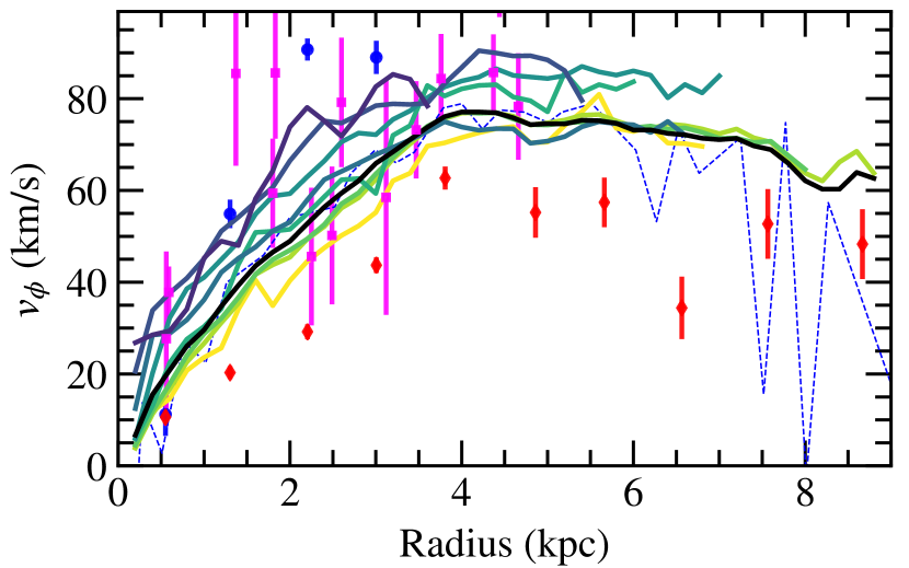
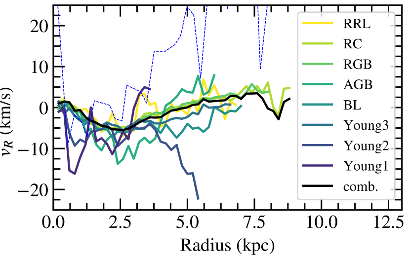
Figure 14: Stellar velocity curves of the LMC. The left and right panels show the rotation curves and radial motions, respectively. Coloured lines are for the eight evolutionary phases and the combined sample, as given by the legend. In the left panel, blue circles, red diamonds and magenta squares are the rotation velocities for the samples of younger and older stars from line-of-sight spectroscopic and HST astrometric measurements published in van der Marel & Kallivayalil (2014). The dashed blue lines are the tangential and radial velocity profiles derived by Wan et al. (2020) from Gaia  DR2  astrometry.

6 Magellanic Bridge and the outskirts of the Magellanic Clouds

One of the most prominent features in the outskirts of two interacting galaxies is the formation of a bridge between them due to tidal forces that strip gas and stars from the least to the most massive galaxy (Toomre & Toomre, 1972). The relative position of the Milky Way with respect to the Magellanic Clouds places us in the privileged position of witnessing the close encounter between the LMC and the SMC, and of studying the Magellanic Bridge.

The stellar characterisation of the structure and kinematics of the Magellanic Bridge has been pursued for a long time, with simulations (e.g. Besla et al., 2012; Diaz & Bekki, 2012) and observations (e.g. Irwin et al., 1985; Harris, 2007; Bagheri et al., 2013; Noël et al., 2013; Carrera et al., 2017). In addition to this expected tidally induced feature, other structures such as plumes, shells or stellar streams can be found in the outskirts of the Magellanic Clouds (e.g. Deason et al., 2017; Mackey et al., 2018; Martínez-Delgado et al., 2019; Navarrete et al., 2019). In this section we show the quality of Gaia  EDR3 in highlighting the Magellanic Bridge and its kinematics, and we show several equally interesting features in the outskirts of the Magellanic Clouds.

The Magellanic Bridge was first detected as an overdensity in HI gas by Hindman et al. (1963). More recently, several studies have tried to follow the connection between the LMC and SMC using samples of stars in different evolutionary phases. Because tidal forces have similar effects on stars and gas, the Bridge would be traced by both a young stellar population with a strong correlation with the HI distribution, and an old population made of stars stripped into the Bridge by the tidal interaction. This is supported by dynamical simulations (e.g. Guglielmo et al., 2014). The stellar Magellanic Bridge was first traced by a population of young stars (Irwin et al., 1985) showing in situ star formation and a strong correlation between the location of the stars and that of HI overdensities (e.g. Skowron et al., 2014). Casetti-Dinescu et al. (2012) selected young OB-type stars in a wide area between the Clouds to study the structure and kinematics of the Bridge using GALEX, 2MASS, and the Southern Proper Motion 4 catalogue. Jacyszyn-Dobrzeniecka et al. (2020b) used Cepheids from the OGLE Collection of Variable Stars to characterise the Magellanic Bridge with young stars, while Bagheri et al. (2013) and Noël et al. (2013) used RGB stars to search for an old counterpart. Spectroscopic confirmation of stripped stars at the SMC side of the Bridge was obtained by Carrera et al. (2017). Very recently, Grady et al. (2020) assembled a catalogue of red giants from Gaia  DR2 from which the authors obtained photometric metallicities using machine-learning methods. Based on the metallicity structure in the Magellanic Bridge, the authors concluded that it is composed of a mixed stellar population of LMC and SMC debris.

In this section we explore the Gaia capabilities of detecting and characterising the Magellanic Bridge using the evolutionary phase samples described in Sect. 2. Because the Magellanic Bridge encompasses the region in which the MC overlap, we have to adopt a modification of the selection described in Sect. 2. This modification takes into consideration that LMC (SMC) stars may extend farther than 20 (11) degrees and overlap with each other spatially and in proper motion. Our query is identical to the one described in Sect. 2, but we queried by HEALpix (NSIDE=8) pixels that have a separation to their centres smaller than 35 (15) degrees from the LMC (SMC) centre. The proper motion selection described in Sect. 2 was performed, but we did not adopt any separation from either of the clouds as a membership criteria. This produced a sample that allowed for overlap in space and velocity and also provided a larger sky-coverage that is useful to explore stellar structures in the outskirts of both clouds. The total number of stars and the number in each stellar phase subsample agrees well with what we reported in Sect. 2, but because we allowed stars to mix in PM and on sky, we obtained numbers that are generally larger by ¡ 1% than in Sect. 2.

To study the Bridge, we defined two populations, one representative of the young population, and the other the RC population in both clouds. The young population was defined as the combination of Young 1_LMC, Young 2_LMC, Young 1_SMC, and Young 2_SMC, that is, inner-joined with the combination of the PM-selected LMC and SMC populations. It contains $167,643$ sources. The RC population is defined in the same way, but using the RC subsamples. It contains $1,806,102$ sources.

In the left panel of Fig. 15 we show a density plot of the Young stellar population in the Bridge region; the connection between the two galaxies is obvious without applying any statistical technique. The morphology of the young Magellanic Bridge is represented by an arched elongated connection between the Magellanic Clouds. In the right panel of Fig. 15 we show the density plot of the RC sample in the Bridge region. The Magellanic Bridge in the RC sample is not so clear, as expected from a more evolved and kinematically hot population, although it has been traced in RC stars by Carrera et al. (2017) at the near side of the SMC using the MAGIC spectroscopic survey. In this case, it is of key importance to remove the Milky Way foreground contamination of RC stars. This exploration has been performed by Zivick et al. (2019) using Gaia  DR2 data and HST proper motions. Belokurov & Erkal (2019) used astrometry and broad-band photometry from Gaia  DR2 , and Schmidt et al. (2020) used data from the VISTA survey of the Magellanic Clouds (Cioni et al., 2011) and Gaia  DR2 to perform a kinematic study of the region around the MC and of the Bridge region.

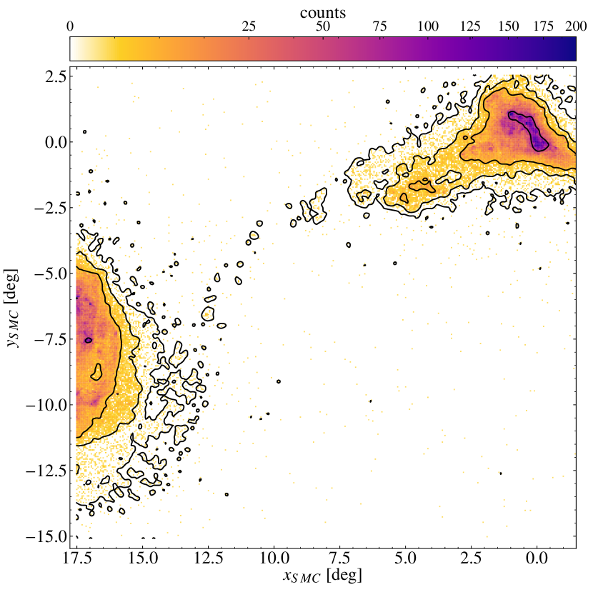
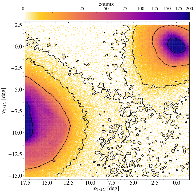
Figure 15: Sky density plot for the Bridge region using the Young1 and Young2 evolutionary phases (left panel) and the RC evolutionary phase (right panel). The bin size is $0.06$ deg in $x$ and $y$. The colour bar is in log scale and the black contours are at the levels $0.1$, $1$, $5,$ and $70$ (young evolutionary phases) and $0.25$, $1.5$, $15,$ and $165$ (RC sample).

In Fig. 16 we specifically use the proper motions included in Gaia  EDR3 to study the kinematic interaction between the Magellanic Clouds. We checked the dynamical attraction of the LMC on the SMC by plotting the vector field of the proper motion of the sources.We separately show the Young 1-2 (left panel) and the RC evolutionary phases (right panel). In contrast to the density plot (see Fig. 15), we clearly observe, using both evolutionaryphases, a coherent motion of stars from the SMC towards the LMC. For young stars the flow moves as we would expect, from the SMC to the LMC along the Bridge (depicted in the background density plot). We emphasise that the excellent quality of the Gaia  EDR3 proper motions allows tracing the interaction between the Magellanic Clouds using a rather simple strategy to separate stars into different phases of evolution.

The high quality of the Gaia  EDR3 proper motions allows confirming a flow of RC stars from the SMC towards the LMC. As mentioned above, the track of an old bridge between the LMC and SMC has recently been pursued using different tracers and strategies. In this demonstration paper we considered only the RC population, which is characteristic of an intermediate to old population, and we did not use a typical $>10$ Gyr old population such as that of the RR Lyrae stars. Recent works have specifically targeted the RR Lyrae stars in the bridge region of the MC (e.g. Belokurov et al., 2017; Clementini et al., 2019; Jacyszyn-Dobrzeniecka et al., 2020a). Based on their selection strategy, Belokurov et al. (2017) claimed an old RR Lyrae bridge for Gaia  DR1 RR Lyraes. The Gaia  DR2 bona fide RR Lyraes and those from the Gaia  EDR3 sample (see Sect. 2) both show a smooth halo-like density distribution (Clementini et al., 2019), however. The Gaia  DR2 accompanying paper was confirmed by Jacyszyn-Dobrzeniecka et al. (2020a) using the extended OGLE catalogue. Evans et al. (2018) stated in a Gaia  DR2 accompanying paper that a suboptimal computation affected the mean magnitude standard deviation given in Gaia  DR1 and Gaia  DR2 (and revised in Gaia  DR3 (Gaia collaboration, Riello et al., 2020)), which may have affected the selection strategy of Belokurov et al. (2017) with only candidate RR Lyrae stars. We show here that a flow of RC stars (see Fig. 16) confirms a bridge composed of an evolved population, and it would have a similar trajectory to that of Belokurov et al. (2017). It is beyond the scope of this paper, however, to make a quantitative comparison.

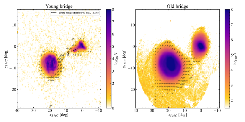
Figure 16: Vector field of the proper motions in the Magellanic Clouds using the Young 1 + Young 2 (left panel) and RC (right panel) samples. The coordinates are centred on the SMC. In the background, to guide the eye of the reader, we show the density in logarithmic scale. The dashed line in the left panel shows the location of the young bridge from Belokurov et al. (2017). The velocity vector field is only shown for bins with more than 10 (200) stars in the Young 1 + Young 2 (RC) sample.

In addition to the Bridge, de Vaucouleurs & Freeman (1972a) showed a wealth of substructure in the outskirts of the Magellanic Clouds in the 1970s. More recently, new shells, plumes, and streams have been detected using different surveys or photometric techniques (e.g. Pieres et al., 2017; Belokurov & Erkal, 2019; Martínez-Delgado et al., 2019). To search for substructures around the Clouds, we adopted a more restrictive selection using the RGB and RC subsamples. First, we corrected for foreground extinction using Schlegel et al. (1998) (with the correction from Schlafly & Finkbeiner (2011)), and we adopted a (Cardelli et al., 1989) extinction curve with $R_{V}=3.1$. This correction is accurate in the outskirts of the Clouds because there is little internal extinction from the LMC and SMC themselves. Second, we built a tighter colour-magnitude selection polygon based on the extinction-corrected RC and RGB samples; in this case, we are stricter in the colour range allowed for these two evolutionary phases as in the RC and RGB samples described in Sect. 2. Additionally, we applied a magnitude cut of G $<$ 19 and selected only stars with a parallax smaller than 0.15. This led to a sample of stars that is less strongly affected by Milky Way foreground, thus allowing us to explore faint substructures in the outskirts; we call this selection LMCout.

In Fig. 17 we show a star count map of the Magellanic Cloud region to highlight the substructure found using Gaia  EDR3. We also annotate a few notable features and show the measured total dispersion and velocity vector map (velocities and dispersion were computed using LMC-centred coordinates). The northern tidal arm (NTA) reported initially by Mackey et al. (2016) is visible in the figure, and this structure is also visible as a velocity low-dispersion feature, with velocities consistent with the LMC main body. A southern tidal arm (STA) (Belokurov & Erkal, 2019) is also evident, which shows indications of being dynamically cold, like the NTA, and the velocities are consistent with those of the LMC. The STA appears to be connected with the SMC through a narrow elongation east of the SMC. The SMC northern overdensity (Pieres et al., 2017) is also evident, and a spatially thinner structure is also seen to be connected to it. In addition to these known substructures, we find a faint overdensity east of the LMC that is visible in the velocity field and density map. We also see a similar structure, but more conspicuous, on the western side of the LMC, close to $y_{LMC}=0$. We note, however, that the features observed near $y_{LMC}=0$ coincide with a region of elevated number of Gaia transits. The eastern feature is also prominent in near-infrared maps from the VISTA Hemisphere Survey (El Youssoufi et al.,submitted).

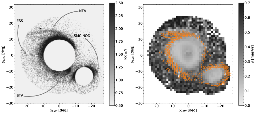
Figure 17: Number count map for the LMCout sample (left): the names of the most notable substructures are given and, for a better visualisation, the inner parts of the LMC and SMC were omitted. Total velocity dispersion map (right): the velocity vector field is shown as orange arrows.

7 Spiral arms in the Large Magellanic Cloud

The LMC is a prototype of barred Magellanic spiral galaxies that are characterised by an off-centre bar and one prominent spiral arm. The dynamical interactions between the LMC and the SMC (e.g. Besla et al., 2016) are probably responsible for this and other spiral features associated with the galaxy (de Vaucouleurs & Freeman, 1972b). A comprehensive study of the morphology of the LMC based on near-infrared observations is given in El Youssoufi et al. (2019), where high spatial resolution maps (0.03 deg²) of stellar populations with different median ages show at least four distinct spiral features. These arms emerge predominantly from the ends of the bar, one in the east extending to the south, and three in the west, one of which extends north, one north-west (the most prominent arm), and the third extends south. The arms are well traced by stellar populations younger than a few million years, while old stellar populations instead show external features that may be associated with a ring-like structure (e.g. Choi et al., 2018). The long-term stability of the prominent spiral arm was studied by Ruiz-Lara et al. (2020) using deep optical photometry to derive the star formation history throughout the galaxy. This structure could have formed a few million years ago at the time when the Magellanic Stream and the Leading Arm formed as well from a close encounter between the LMC and the SMC. The authors concluded that the distribution of HI gas and the coherent star formation at the location of the arm support this scenario. In this section we show that the spiral structure of the LMC can be highlighted and studied with the Gaia  EDR3 data.

7.1 Basic properties as a function of evolutionary phase

We discuss here the appearance of the spiral arms of the LMC using the evolutionary phase samples as proxies for age-selected samples (see Sect. 2.3). In Fig. 18 we show the maps obtained in the LMC for these samples. The maps were constructed considering a region $20\times 20$ deg² around the galaxy, applying a Gaussian smoothing and sampling with $400\times 400$ pixels, each with a dimension of $3\arcmin\times 3\arcmin$. Each map was normalised to the total number of objects. The figure shows that the main structures of the LMC, that is, the bar and the spiral arms, are clearly outlined by BL stars, objects with ages in the range of 50-350 Myr. We therefore chose this population as a reference for the comparison of the spiral structure(s) in other stellar populations of different ages.

Because the differential maps of the BL with respect to Young 1 and Young 2 were similar, we merged these two evolutionary phases into a single sample. We refer to this merged sample as the young population of stars with age $<400$ Myr, which is shown in the middle top panel of Fig. 18. Similar considerations applied to the RC, RGB, and RRL populations, all older than 1 Gyr, and we refer to these merged evolved populations as the old population. The relative differential map is shown in the lower panel of Fig. 18. Finally, the differential map with respect to the Young 3 population (MS stars with ages $<1-1.5$ Gyr) is shown in the middle panels of the same figure.

The analysis of the top panel in Fig. 18 reveals that the young population is more concentrated around the bar and an inner northern arm, showing a clumpy structure. The residual map with respect to the BL shows that this latter population has an excess of stars along the bar, in the spiral feature at the end of the bar, and in an outer north-east arm (referred to as the eastern arm hereafter).

The comparison of BL and Young 3 populations shows that the two populations are distributed in a very similar way, even though the BL still displays an excess along the bar, especially in the eastern region, where it shows a concentration superior to any other population in the LMC ($\Delta{\rm RA},\Delta{\rm DEC}\sim-3\degr,-1\degr$). The older populations of the LMC have a homogeneous distribution; the star density decreases smoothly from the centre to the outskirts of the LMC. The lower density along the bar is caused by the Gaia incompleteness in this crowded region. The difference with the BL population again shows an excess of stars along the bar and the above-mentioned clump in the eastern bar, but these features might in part be justified by the incompleteness of old populations in the more central region of the bar. In contrast, the excess of BL stars in the inner and outer arms appears to be genuine.

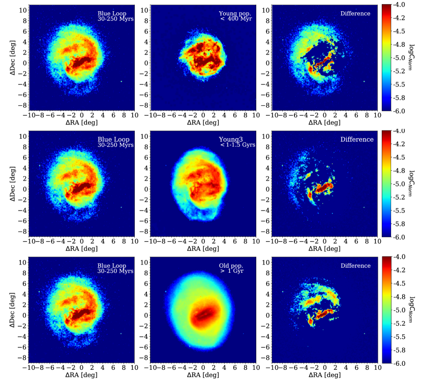
Figure 18: Differential density maps for different stellar populations in the LMC. The left column shows the density map in the BL evolutionary phase. The middle panels from top to bottom display the density maps of the young phase, i.e. stars with age $<$ 400 Myr, Young 3 phase, i.e. main- sequence stars with age $1-1.5$ Gyr, and old phase, i.e. stars with age $>$ 1 Gyr. The right column depicts the normalised difference between the left and middle panel maps, shown with a logarithmic stretch.

7.2 Strength and phase of the density perturbations

To be more quantitative on the effect of the bar and spiral structure on the stellar density, we performed discrete fast Fourier transforms (FFTs) of density maps of the BL and the combined samples. For this purpose, we again used $400\times 400$ pixels maps, but at 0.04° sampling, as in Sect. 5.2. This allowed us to estimate the properties of any asymmetries in the density maps.

Because the apparent dominant modes of perturbations are the bar (second-order perturbation), the inner spiral structure starting at the end of the bar, and the eastern outer arm (first-order perturbation), we present results up to the second-order harmonics, although the discrete FFTs yield as many orders as existing pixels in a vector. Therefore the analytic form equivalent to the discrete FFT applied to a density map is $\Sigma(R,\phi)=\sum_{k}\Sigma_{k}(R)\cos k(\phi-\phi_{k}(R))$, where $k$ is an integer, $\phi$ the azimuthal angle in the plane of the LMC with the reference $\phi=0$ chosen aligned to the photometric major axis of the disc ($\Omega_{\rm phot}$), $\Sigma_{0}$ the axisymmetric surface density, and $\Sigma_{k}$ and $\phi_{k}$ are the amplitude and phase of the $k$-th asymmetry.

We measured $\Omega_{\rm phot}$ by isophotal ellipse fitting to the stellar surface density map of the combined sample. To avoid confusion with Sect. 5, which gives radii in a kinematic frame oriented along the kinematic position angle of $\Omega=310\degr$, we refer to $R_{\rm phot}$ as the galactocentric radius measured in the photometric frame, which is aligned on $\Omega_{\rm phot}$. With this, we find the bar semi-major axis at a position angle of $\sim 105\degr$, and define the one for the disc as that of the average value in the radial range $R_{\rm phot}=3.5-7.5$ kpc, which is $\Omega_{\rm phot}\sim 10\degr$. The photometric major axis therefore differs by $\sim 60\degr$ from the kinematic major axis. A similar discrepancy has been reported in van der Marel et al. (2002).

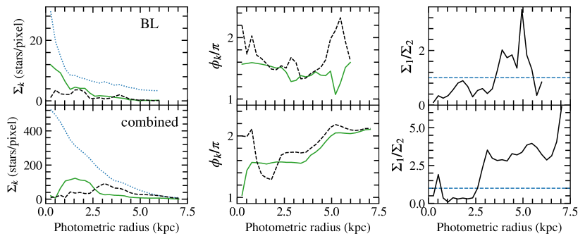
Figure 19: Results of the Fourier transform of stellar density maps of the LMC for the BL and the combined samples (upper and bottom panels, respectively). The left and middle panels show the amplitude and phases of the first- and second-order asymmetries (dashed black and solid green lines, respectively). The axisymmetric density is shown as a dotted blue line. The right panel shows the $k=1$ perturbation over the bisymmetry strength ratio. The galactocentric radius is given here in the photometric frame, with $\Omega_{\rm phot}=10\degr$ as the reference photometric position angle.

Fig. 19 shows the results of the Fourier transforms. We restrict the analysis to $R_{\rm phot}\leq 7.5$ kpc. The axisymmetric density profile of BL stars is more centrally peaked than that of the whole sample. At the peak of $\Sigma_{1}$ and $\Sigma_{2}$, the strengths of the lopsided outer spiral arm ($k=1$) and bisymmetry ($k=2$) reach 60% and 40% the amplitude of the axisymmetric mode for the combined sample, and 48% and 40% for the BL stars. At $R_{\rm phot}>5.5$ kpc, the strength of the lopsided spiral is similar to the axisymmetric value. The lopsidedness and bisymmetry perturbations are therefore not negligible in the LMC.

Both samples show that the dominant perturbation at low radius is the bisymmetric mode ($R_{\rm phot}<3.5$ kpc for BL stars, $R_{\rm phot}<2.5$ kpc for the combined stars), while the lopsided mode dominates at larger radii. In the inner kpc, the $\Sigma_{2}$ profile of the whole sample presents a dearth of stars that is lacking in the density map of younger stars. This is caused by the incompleteness of Gaia in this crowded region of the LMC disc. This dearth of stars also affects the inner profile of $\phi_{2}$ for all stars as a central phase dip.

The orientation of the inner $k=2$ perturbation does not change much in the inner disc, with a bar oriented with a phase angle of $1.6\pi$ rad (modulo $\pi$) for both samples. The $k=2$ spiral structure of BL stars has a phase angle of $1.4\pi$ rad ($R_{\rm phot}>3$ kpc), while that for the combined sample smoothly increases to $\sim 2.1\pi$ rad for $R_{\rm phot}=3.5-5.2$ kpc, then remains constant out to the last radius. The phase angles of the lopsided mode continuously vary as a function of radius, and the two stellar samples present different shapes of $\phi_{1}$. The similar shape of $\phi_{1}$ and $\phi_{2}$ at $R_{\rm phot}>2.5$ kpc for the combined sample of stars is remarkable, and the amplitudes only differ by less than 0.2$\pi$. The outer spiral structure in the LMC combined sample is thus made of two modes that are tightly coupled.

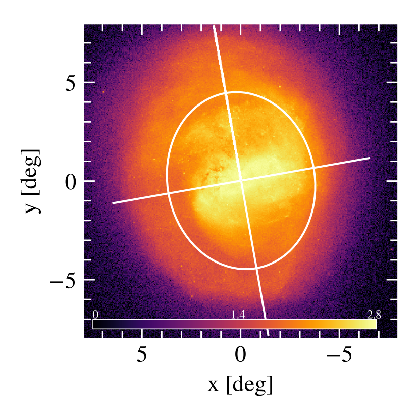
Figure 20: Stellar density map of the combined sample of the LMC. The lopsided eastern spiral arm is located beyond $R_{\rm phot}=3.8$ kpc (shown as an ellipse). The perpendicular axes show the orientation of the photometric major and minor axes (Sect. 7.2). The density scale shown by the colour bar is logarithmic; the values indicate the star count in pixels.

7.3 Across and along streaming motions in the eastern spiral arm

The LMC velocity fields have been shown to exhibit variations stemming from the juxtaposition of an observational sawtooth-like pattern inherent to Gaia, and others likely caused by intrinsic perturbations of the gravitational potential of the LMC (Sect. 5.2). Here we illustrate in a simple way the variation of $v_{\phi}$ and $v_{R}$ along and across the dominant outer $k=1$ spiral arm to the east in the combined sample.

To isolate the effects of the outer arm better, we only considered the region where the inner $k=2$ mode becomes negligible, that is, all pixels located at $R_{\rm phot}>3.8$ kpc (Fig. 20). We built azimuth-radius diagrams of the stellar density and tangential and radial velocities by calculating average star counts, $v_{\phi}$ and $v_{R}$  in bins of 5° size in azimuthal angle, and 63 pc in radius (Fig. 21). The horizontal variation is thus a good proxy of the streaming of $v_{\phi}$ and $v_{R}$ along the eastern spiral arm, while the vertical axis is a good proxy for the velocity variation across the spiral arm.

The density of the spiral arm is strongly asymmetric as a function of azimuthal angle, caused by its lopsided nature. The uppermost isocontour of density (mean star count of $\sim 20$ stars) approximately delineates the maximum radial extent of the spiral arm, which extends to $R_{\rm phot}\sim 7$ kpc along the photometric major axis ($\phi=0\degr$) to $R_{\rm phot}\sim 5.4$ kpc ($\phi=240\degr$). The highest densities around $\phi=300\degr$ at lower radii correspond to regions of the LMC that are part of the inner spiral structure, thus not strictly belonging to the outer lopsided eastern arm.

Along the horizontal axis, $v_{\phi}$ is maximum in higher density regions and minimum in lower density regions. When we consider pixels below the outermost contour, the azimuthal streaming in the arm is relatively constant ($60\lesssim v_{\phi}\lesssim 90$ km s^-1). An exception to this occurs at $R\sim 6$ kpc owing to the lower values of $v_{\phi}$ around $\phi=100\degr$. As the pixels above the uppermost contour likely probe stars beyond the spiral arm, the difference in colours between pixels below (redder) or above (bluer, $v_{\phi}<60$ km s^-1) the uppermost contour clearly shows the effect of the arm on $v_{\phi}$ in the azimuthal direction. The radial velocity also varies significantly with azimuth. It is stronger in higher density regions around $\phi=50\degr$ and $\phi=200\degr$ ($v_{R}>-10$ km s^-1) and in lower density regions for $100<\phi<180\degr$ , but with inward motions ($v_{R}<-10$ km s^-1). The noise in $v_{R}$ is higher outside the arm at large radii.

Along the vertical axis, $v_{\phi}$ is observed to decline with radius across the spiral arm, and the decrease is not complete at the same rate for different azimuthal angles. This implies a wide diversity of shapes and amplitudes in the LMC rotation curve as a function of azimuth. We have observed this trend in the $v_{\phi}$ map of Sect. 5.2. The radial velocity also varies across the spiral arm, but there appears to be no clear rule, unlike for $v_{\phi}$. For example, the peak of $v_{R}$ at $\phi=50\degr$ occurs at $R_{\rm phot}=5.5-6$ kpc, thus beyond the location of the density peak ($R_{\rm phot}\lesssim 4.5$ kpc). However, at an angle of for instance $\phi=200\degr$, the opposite is observed, with larger $v_{R}$ for higher density regions of this azimuthal angle ($R_{\rm phot}\lesssim 4.5$ kpc).

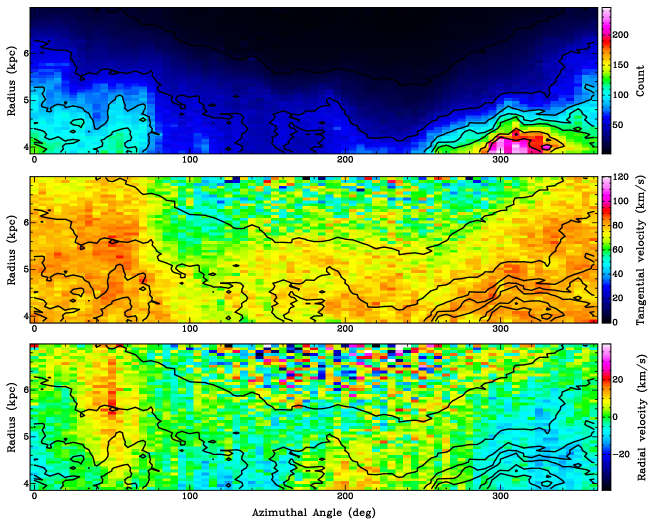
Figure 21: Streaming motions across and along the eastern spiral arm of the LMC. The azimuth-radius diagrams show the stellar density (top panel), the tangential velocity (middle panel), and radial velocity (bottom panel). Contours represent the stellar density shown in the upper panel.

8 Conclusions

Using the new Gaia  EDR3 data, we studied the structure and kinematics of the Magellanic Clouds with a new basis. The increased completeness and precision of the new release have allowed us to improve upon previous results using Gaia  DR2 , although (by design, because this is just a demonstration paper) we have certainly barely scratched the potential of the new data for the study of the Clouds.

In Sect. 3 we compared the Gaia  DR2 and Gaia  EDR3 data in the region of the LMC and SMC, showing the improvement in the astrometry and photometry from one release to the other. Not only the precision has increased, but the systematic effects are significantly reduced. The reduced crowding effects in the photometry are particularly relevant for the central regions of the Clouds.

We have explored the use of the astrometric data for the determination of the 3D structure of the LMC. Our attempts to use Bayesian modelling to reconstruct the geometry of the system have shown that despite the significant improvements in Gaia  EDR3, the systematic effects still present on the parallaxes (the regional zero-points discussed in Gaia collaboration, Lindegren et al. (2020a)) distort most of the signal of the 3D structure of the LMC (in the astrometry), and that there is not enough information in the summary statistics used by our approximate Bayesian method to simultaneously infer the local parallax zero-point variations and the geometry of the LMC. However, we do not rule out that it may be possible to determine this geometry by adding additional external restrictions and/or finding an optimal way to include additional information of the density distribution of the stars in the LMC area.

Our kinematic modelling of the proper motions has allowed us to derive radial and tangential velocity maps and global profiles for the LMC. This is the first time to our knowledge that the two planar components of the ordered and random motions are derived for multiple stellar evolutionary phases in a galactic disc outside the Milky Way. We show that younger stellar phases rotate faster than older ones. This is a clear effect of the asymmetric drift on the stellar kinematics. We have also been able to find the rotational centre of the stars in the LMC and showed that is significantly offset from the rotational centre of the H i gas.

On the other hand, we showed that the radial velocity is mostly negative in the inner 5 kpc, and inward radial motions are stronger in the bar region for younger stars. This velocity varies strongly as a function position with respect to the bar, and therefore to some extent reflects streaming motions along the bar. We observed asymmetric radial and tangential motions in the disc, such as those across and along the large-scale outer spiral arm of the LMC, in which the tangential velocity is larger in higher stellar density regions of the arm, and lower at lower density. There appears to be no clear rule in the streaming of the radial motion as a function of the position in the arm, however.

We showed that the radial and tangential random motions decrease from the disc centre out to the outskirts, but not at the same rate in the evolutionary phases. Older stars lie in a dynamically hotter disc than younger stars. While we have found higher velocity dispersions aligned with the bar in all stellar phases for both components, we also found evidence that only the radial component of more evolved stars exhibits a central feature of higher amplitude, which is oriented perpendicular to the bar.

Our analysis of the stellar density maps has shown more concentrated and clumpier distributions for younger stars in the bar and inner spiral structure(s) than older disc stars. Analysis of Fourier harmonics of density maps also revealed that the inner disc is perturbed predominantly by bisymmetries, the bar and spiral arms, while the outer disc is perturbed by a dominant lopsided spiral arm. The peak strengths of these perturbations can be as high as 40% to 60% of the axisymmetric amplitude in the inner region, and higher in the disc outskirts for the lopsidedness.

Finally, we carried out a specific study of the Magellanic Bridge. Using two different evolutionary phases (the young and RC samples), we were able to trace the density and velocity flow of the stars from the SMC towards the LMC following the Bridge. We showed that it apparently wraps around the LMC, connecting with the young southern arm-like structure of the galaxy. The quality of the Gaia  EDR3 proper motions also allowed us to confirm the bridge in the RC evolutionary phase, at a position slightly shifted from that of the young evolutionary phase. Additionally, we were able to study the outskirts of both Magellanic Clouds and detected some well-known features, such as the north and south tidal arms of the LMC and the northern overdensity of the SMC. Our data also suggests a faint overdensity east of the LMC, which has only recently been reported with the help of near-infrared maps (El Youssoufi, private communication).

Appendix A Sky plots of the samples used

This appendix provides some additional figures complementary to the main text, collected here to avoid cluttering the main body and facilitate reading of the paper.

First, in Fig. 22 we illustrate the joint sky distribution of our two (LMC and SMC) basic clean samples. The selection radius for both clouds is clearly visible. Following this map, the next figures show the distribution of the mean $G$ magnitude (Fig. 23), mean $G_{\rm BP}-G_{\rm RP}$ (Fig. 24), the variation of this mean between Gaia  DR2 and Gaia  EDR3 (Fig. 25), and the mean parallax (Fig. 26).

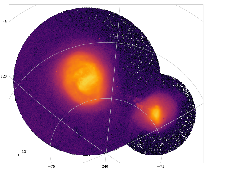
Figure 22: Source density in the two circular areas with a radius of 20° and 11°, centred on the LMC and SMC. Only the 12.4M sources selected as potential members are included, and the criteria are therefore slightly different for the two circles.

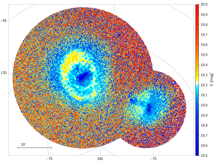
Figure 23: Mean $G$ magnitude in the LMC and SMC.

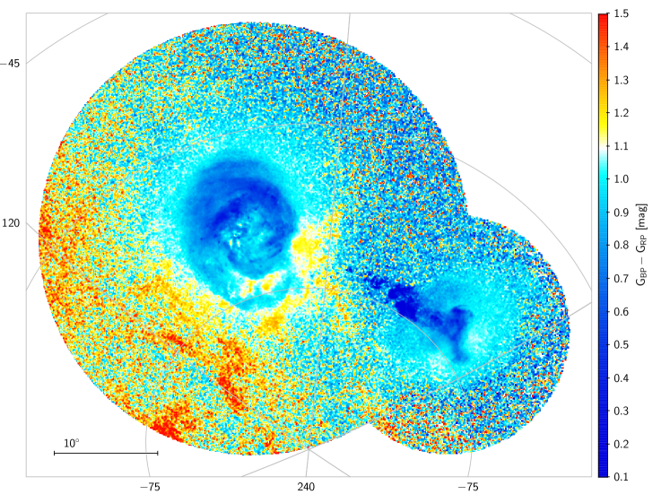
Figure 24: Mean colour, $G_{\rm BP}-G_{\rm RP}$ in the LMC and SMC.

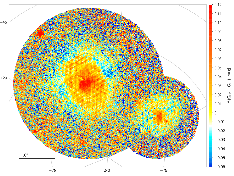
Figure 25: Mean change in colour, $G_{\rm BP}-G_{\rm RP}$, in Gaia  DR2  and Gaia  EDR3 for sources in the LMC and SMC. Positive values mean that the sources are now redder.

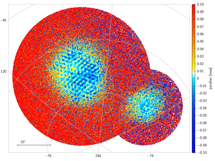
Figure 26: Mean parallax for sources in the LMC and SMC. No corrections have been applied to the parallaxes.

Next, we provide plots of the sky distribution for each one of our evolutionary phase samples; the plots show that each sample traces different structures of the clouds. Fig. 27 contains the plots for the LMC and Fig. 28 those for the SMC.

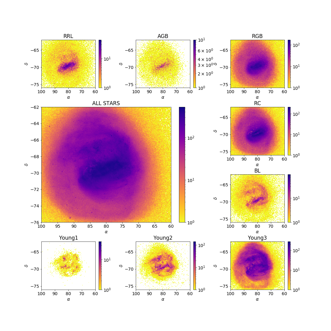
Figure 27: Sky density plots for the complete LMC clean sample and the different evolutionary phase subsamples.

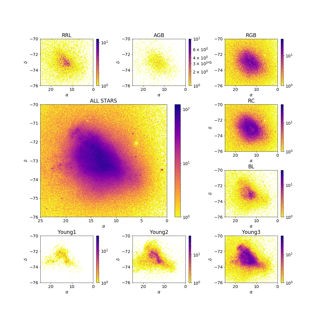
Figure 28: Sky density plots for the complete SMC clean sample and the different evolutionary phase subsamples.

Appendix B LMC velocity maps and profiles

We include here several figures that complement the analysis of the kinematics of the LMC presented in Sect. 5. Figures 29 to 32 present the velocity maps of the LMC (azimuthal and radial velocities, mean values, and dispersion) for the eight evolutionary phases and the combined sample of stars. Finally, Fig. 33 presents the velocity profiles of the LMC (as a function of the distance to its centre) traced using the different populations defined by our evolutionary phases.

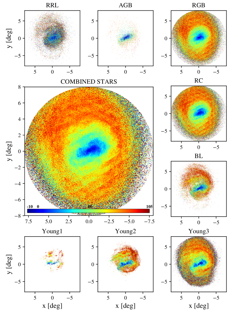
Figure 29: Azimuthal velocity maps $v_{\phi}$ of the LMC for the combined sample (main panel) and the various evolutionary phases. The linear velocity scale shown by the colour bar in the main panel is the same in all subpanels and has been chosen to highlight velocity patterns better.

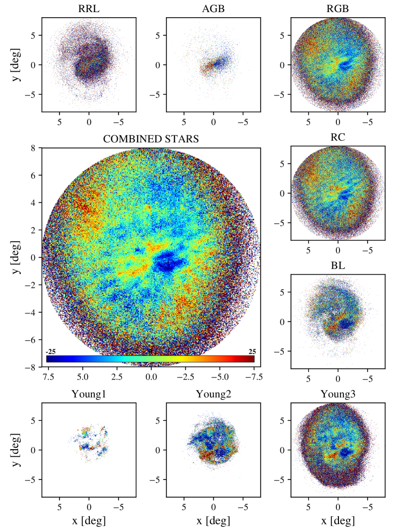
Figure 30: Radial velocity maps $v_{R}$ of the LMC for the combined sample (main panel) and the various evolutionary phases. The linear velocity scale shown by the colour bar in the main panel is the same in all subpanels and has been chosen to highlight velocity patterns better.

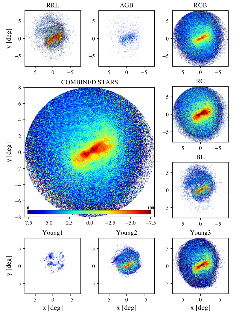
Figure 31: Azimuthal velocity dispersion maps $\sigma_{\phi}$ of the LMC for the combined sample (main panel) and the various evolutionary phases. The linear velocity scale shown by the colour bar in the main panel is the same in all subpanels and has been chosen to highlight velocity patterns better.

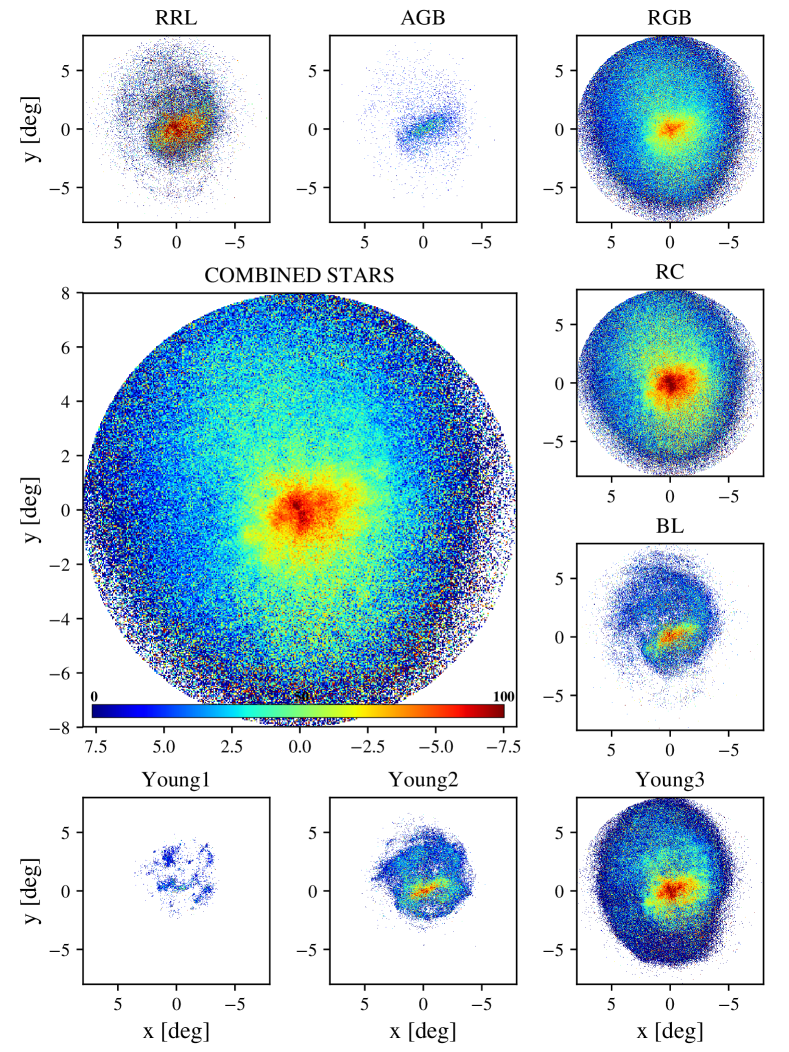
Figure 32: Radial velocity dispersion maps $\sigma_{R}$ of the LMC for the combined sample (main panel) and the various evolutionary phases. The linear velocity scale shown by the colour bar in the main panel is the same in all subpanels and has been chosen to highlight velocity patterns better.

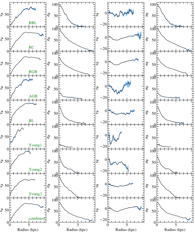
Figure 33: Velocity profiles of the LMC. Rotation curve ($v_{\phi}$), tangential velocity dispersion ($\sigma_{\phi}$), radial velocity ($v_{R}$), and radial velocity dispersion ($\sigma_{R}$) from left to right for each stellar evolutionary phase (from top to bottom). Velocities are in km s^-1. The bottom row is the result for the combined sample. The blue shaded areas correspond to the uncertainties.