QCD evolution of the gluon Sivers function in heavy flavor dijet production at the Electron-Ion Collider

Abstract

Using Soft-Collinear Effective Theory, we develop the transverse-momentum-dependent factorization formalism for heavy flavor dijet production in polarized-proton-electron collisions. We consider heavy flavor mass corrections in the collinear-soft and jet functions, as well as the associated evolution equations. Using this formalism, we generate a prediction for the gluon Sivers asymmetry for charm and bottom dijet production at the future Electron-Ion Collider. Furthermore, we compare theoretical predictions with and without the inclusion of finite quark masses. We find that the heavy flavor mass effects can give sizable corrections to the predicted asymmetry.

1 Introduction

In recent years, one of the most important forefronts of hadron physics has been the exploration of the three-dimensional (3D) partonic structure of nucleons in momentum space. Such 3D information is encoded in the so-called transverse-momentum-dependent parton distribution functions (TMD PDFs), which can further inform us about the confined motion of partons in the nucleon, as well as the correlation between their spins, momenta, and the spin of the nucleon Accardi:2012qut . Thanks to semi-inclusive deep inelastic scattering (SIDIS), a great deal of progress has been made in probing and extracting the TMD PDFs of quarks–however, information regarding those of gluons is still largely unknown experimentally. Exploring and measuring gluon TMD PDFs is one of the primary goals for the future Electron Ion Collider (EIC).

Among the gluon TMD PDFs, the so-called gluon Sivers function is regarded as one of the “golden measurements” at the future EIC Accardi:2012qut . The gluon Sivers function encapsulates the quantum correlation between the gluon’s transverse momentum inside the proton and the spin of the proton, thus providing 3D imaging of the gluon’s motion. Quite a few processes have been proposed to probe the gluon Sivers function at the EIC, including heavy quark pair production Boer:2016fqd , heavy quarkonium production Yuan:2008vn ; Mukherjee:2016qxa ; Rajesh:2018qks ; Bacchetta:2018ivt ; Boer:2020bbd , and quarkonium-jet production DAlesio:2019qpk , as well as back-to-back dihadron and dijet production Boer:2011fh . The feasibility of measuring the gluon Sivers function in the above scenarios has been studied in Zheng:2018ssm , where the authors use the PYTHIA event generator Sjostrand:2006za and the reweighting method of Airapetian:2010ac to investigate the spin asymmetry. They conclude that dijet production is the most promising channel for probing gluon Sivers effects, where the selection of a sufficiently small-$x$ value suppresses the contribution of the quark channel and the corresponding quark Sivers function. In this paper, we discuss spin asymmetry in the process of heavy flavor (HF) dijet production, where the contribution of the quark Sivers function is further suppressed compared to that of the light flavor dijet case.

An intriguing feature common to both quark and gluon Sivers functions is that they depend non-trivially on the processes in which they are probed. A well-known example of the process-dependence of the quark Sivers function is its sign change between SIDIS and Drell-Yan processes Brodsky:2002cx ; Collins:2002kn ; Boer:2003cm . Similarly, it has been demonstrated that the gluon Sivers function for the process of back-to-back diphoton production in $p+p$ collisions, $p^{\uparrow}p\to\gamma\gamma X$, carries a sign opposite to that of dijet production in $e+p$ collisions, $ep^{\uparrow}\rightarrow e^{\prime}jjX$: $f_{1T,g}^{\perp\left[ep^{\uparrow}\rightarrow e^{\prime}jjX\right]}\left(x,k_{T}\right)=-f_{1T,g}^{\perp\left[p^{\uparrow}p\rightarrow\gamma\gamma X\right]}\left(x,k_{T}\right)$ Boer:2016fqd . In Buffing:2013kca , it was demonstrated that the gluon Sivers function in any process can be expressed in terms of two “universal” functions with calculable color coefficients for each partonic subprocess. We briefly discuss such a process-dependence for HF dijet production below. For a comprehensive review on gluon TMD PDFs, see Boer:2015vso ; Arbuzov:2020cqg .

So far, studies of the gluon Sivers function at the EIC are mostly performed within the leading-order (LO) parton model, without considering the impact of QCD evolution. The effects of resummation for back-to-back light flavor dijet production in the unpolarized DIS process have been investigated in Banfi:2008qs , where the authors apply the $p_{T}$-weighted recombination scheme Ellis:1993tq in defining the jet axis to avoid the theoretical complexity arising from non-global logarithm (NGL) resummation Dasgupta:2001sh . A similar idea is used to study single inclusive jet production in the Breit frame at the EIC in Gutierrez-Reyes:2018qez ; Gutierrez-Reyes:2019vbx . Recently, following the same Soft-Collinear Effective Theory (SCET) framework utilized in Buffing:2018ggv ; Liu:2018trl ; Liu:2020dct ; Chien:2019gyf ; Kang:2020xez , the TMD factorization formula for light flavor dijet production at the EIC has been derived delCastillo:2020omr , where the azimuthal-angle-dependent soft function, describing the interaction between two final-state jets through the exchange of low-energy gluons, is analytically calculated at one-loop order. For HF jet production in the kinematic region of comparable jet and heavy quark masses, a new effective theory framework is needed. In this work, we provide such a framework and derive the TMD factorization formula.

The remainder of this paper is organized as follows. In Sec. 2, we detail the factorization framework required to carry out resummation in the back-to-back region where the transverse momentum imbalance of the HF dijet is small. In Sec. 3, we present numerical results for charm and bottom dijet production in both unpolarized and transversely-polarized-proton-electron scattering. We summarize our findings and give an outlook for future investigations in Sec. 4.

2 Factorization and resummation formula

In this section, we start with the kinematics for HF dijet production in $e+p$ collisions. We then provide the TMD factorization formalism with explicit expressions for all the relevant factorized ingredients.

\begin{overpic}[width=455.3023pt]{fig.pdf} \end{overpic}

Figure 1: HF dijet production in electron-proton collisions, as stated in Eq. (1).

2.1 Kinematics

As shown in Fig. 1, we consider HF dijet production in the polarized-proton-electron scattering process

$$e(\ell)+N(P,\bm{S}_{T})\to e(\ell^{\prime})+J_{\mathcal{Q}}(p_{J})+J_{\bar{\mathcal{Q}}}(p_{\accentset{\rule{2.79996pt}{0.8pt}}{J}})+X\,,$$ (1)

where $\bm{S}_{T}$ is the transverse spin of the polarized proton with momentum $P$ and $\ell$ ($\ell^{\prime}$) is the momentum of the incoming (outgoing) electron. At LO, HF dijets are produced via the $\gamma^{*}g\to\mathcal{Q}\bar{\mathcal{Q}}$ process. The HF quark $\mathcal{Q}$ and antiquark $\bar{\mathcal{Q}}$ initiate the observed HF jets $J_{\mathcal{Q}}$ and $J_{\bar{\mathcal{Q}}}$ with momentum $p_{J}$ and $p_{\accentset{\rule{2.79996pt}{0.8pt}}{J}}$, respectively. In this paper, we choose to work in the Breit frame so that both the virtual photon (with momentum $q=\ell-\ell^{\prime}$) and the beam proton scatter along the $z$-axis. For convenience, we define the following variables commonly used in DIS,

$$Q^{2}=-q^{2}\,,\quad x_{B}=\frac{Q^{2}}{2P\cdot q}\,,\quad y=\frac{P\cdot q}{P\cdot\ell}\,.$$ (2)

We may further note that $Q^{2}=x_{B}\,y\,S_{\ell P}$, where $S_{\ell P}=(\ell+P)^{2}$ denotes the electron-proton center-of-mass energy. In a fashion analogous to SIDIS, we also define the kinematic variable $z=P\cdot p_{J}/P\cdot q$, which gives the momentum fraction of the photon carried by the jet $J_{\mathcal{Q}}$. At LO, the four-momenta of the incoming and outgoing particles are expressed as

$$q^{\mu}=\frac{Q}{2}(n^{\mu}-\bar{n}^{\mu})\,,\quad P^{\mu}=\frac{Q}{x_{B}}\frac{\bar{n}^{\mu}}{2}\,,$$

$$\ell^{\mu}=\frac{Q}{y}\frac{n^{\mu}}{2}+Q\frac{1-y}{y}\frac{\bar{n}^{\mu}}{2}+\ell_{t}^{\mu}\,,\quad\ell^{\prime\mu}=Q\frac{1-y}{y}\frac{n^{\mu}}{2}+\frac{Q}{y}\frac{\bar{n}^{\mu}}{2}+\ell_{t}^{\mu}\,,$$

$$p_{J}^{\mu}=zQ\frac{n^{\mu}}{2}+\frac{p_{T}^{2}}{zQ}\frac{\bar{n}^{\mu}}{2}+p_{t}^{\mu}\,,\quad p_{\accentset{\rule{2.79996pt}{0.8pt}}{J}}^{\mu}=(1-z)Q\frac{n^{\mu}}{2}+\frac{p_{T}^{2}}{(1-z)Q}\frac{\bar{n}^{\mu}}{2}-p_{t}^{\mu}\,,$$ (3)

where we have introduced two light-like vectors, $n^{\mu}=(1,0,0,1)$ and $\bar{n}^{\mu}=(1,0,0,-1)$, and define $p_{t}^{\mu}$ such that $p_{t}^{\mu}{p_{t}}_{\mu}=-p_{T}^{2}$ with $\bm{p}_{T}=p_{T}(\cos\phi_{J},\sin\phi_{J})$. We denote transverse momenta relative to the photon-proton beam by the subscript $T$, while that relative to the jet direction is given the subscript $\perp$. Here, we assume $p_{T}^{2}\gg m_{\mathcal{Q}}^{2}$ and take $p_{J}^{2}=p_{\accentset{\rule{2.79996pt}{0.8pt}}{J}}^{2}=0$. This allows us to derive the factorized cross section in the following section. Lastly, the parton-level Mandelstam variables can be defined as

$$\hat{s}\equiv(p_{g}+q)^{2}=(p_{J}+p_{\accentset{\rule{2.79996pt}{0.8pt}}{J}})^{2}=\frac{p_{T}^{2}}{z(1-z)}\,,$$ (4)

$$\hat{t}\equiv(p_{g}-p_{J})^{2}=(q-p_{\accentset{\rule{2.79996pt}{0.8pt}}{J}})^{2}=-\frac{Q^{2}x\,z}{x_{B}}\,,$$ (5)

$$\hat{u}\equiv(p_{g}-p_{\accentset{\rule{2.79996pt}{0.8pt}}{J}})^{2}=(q-p_{J})^{2}=-\frac{Q^{2}x\,(1-z)}{x_{B}}\,,$$ (6)

where $x$ is the momentum fraction of the proton carried by the gluon, and is given by

$$x=\frac{x_{B}D}{Q^{2}z(1-z)},\quad\text{ with }\quad D=Q^{2}z(1-z)+p_{T}^{2}\,.$$ (7)

2.2 Factorization formula

In the Breit frame, we define the dijet imbalance as $\bm{q}_{T}=\bm{p}_{JT}+{\bm{p}}_{\accentset{\rule{2.79996pt}{0.8pt}}{J}T}$. For this paper, we examine the back-to-back configuration where $q_{T}\ll{p}_{\accentset{\rule{2.79996pt}{0.8pt}}{J}T}\sim p_{JT}\equiv p_{T}$. Furthermore, we work in the kinematic regime where $m_{\mathcal{Q}}\lesssim p_{T}R\ll p_{T}$, with $R$ denoting the jet radius. Overall, in the region with the scale hierarchy as $q_{T}R\ll q_{T}\lesssim m_{Q}\lesssim p_{T}R\ll p_{T}$, the factorized expression for the proton-spin-independent cross section is given by

$$\frac{d\sigma^{UU}}{dQ^{2}dyd^{2}\bm{p}_{T}dy_{J}d^{2}\bm{q}_{T}}= H(Q,y,p_{T},y_{J},\mu)\int d^{2}\lambda_{T}\,d^{2}k_{T}\,d^{2}l_{\mathcal{Q}T}\,d^{2}l_{\bar{\mathcal{Q}}T}S(\bm{\lambda}_{T},\mu,\nu)$$ (8)

$$\times\delta^{(2)}(\bm{\lambda}_{T}+\bm{k}_{T}+\bm{l}_{\mathcal{Q}T}+\bm{l}_{\bar{\mathcal{Q}}T}-\bm{q}_{T})\,f_{g/N}\left(x,k_{T},\mu,\zeta/\nu^{2}\right)\,$$

$$\times J_{\mathcal{Q}}(p_{T}R,m_{\mathcal{Q}},\mu)\,S_{\mathcal{Q}}^{c}(\bm{l}_{\mathcal{Q}T},R,m_{\mathcal{Q}},\mu)\,J_{\bar{\mathcal{Q}}}(p_{T}R,m_{\mathcal{Q}},\mu)\,S_{\bar{\mathcal{Q}}}^{c}(\bm{l}_{\bar{\mathcal{Q}}T},R,m_{\mathcal{Q}},\mu)\,.$$

Above, $y_{J}$ is the rapidity of the HF jet $J_{\mathcal{Q}}$ and is related to the kinematic variable $z$ through the relation $z=e^{y_{J}}p_{T}/Q$. In the factorization formula Eq. (8), $S$ denotes the soft function while $f_{g/N}$ is the unpolarized gluon TMD PDF. Their perturbative one-loop expressions can be found in Sec. 2.4. In the third line of Eq. (8), $J_{\mathcal{Q}}$ and $S_{\mathcal{Q}}^{c}$ are the massive quark jet and collinear-soft functions, which differ from the corresponding functions utilized in light jet production Buffing:2018ggv ; Liu:2018trl ; Liu:2020dct ; Chien:2019gyf ; Kang:2020xez . In Secs. 2.5 and 2.6, we present their explicit calculations at next-to-leading order (NLO). The variables $\bm{k}_{T}$, $\bm{\lambda}_{T}$, and $\bm{l}_{T}$ label the transverse momenta associated with the collinear, soft, and collinear-soft modes. Finally, $\mu$ and $\nu$ are the factorization and rapidity scales, respectively, while $\zeta$ is the Collins-Soper parameter Collins:2011zzd ; Ebert:2019okf . In the derivation of the above factorization formula we apply the narrow jet approximation with $R\ll 1$. However, as shown in Jager:2004jh ; Mukherjee:2012uz ; Dasgupta:2016bnd ; Liu:2018ktv this approximation works well even for fat jets with radius $R\sim\mathcal{O}(1)$, and the power corrections of $\mathcal{O}(R^{2n})$ with $n>0$ can be obtained from the perturbative matching calculation.

Fourier transforming to $b$-space, the factorized cross section becomes

$$\frac{d\sigma^{UU}}{dQ^{2}dyd^{2}\bm{p}_{T}dy_{J}d^{2}\bm{q}_{T}}= H(Q,y,p_{T},y_{J},\mu)\int\frac{d^{2}b}{(2\pi)^{2}}e^{i\bm{b}\cdot\bm{q}_{T}}S(\bm{b},\mu,\nu)\,f_{g/N}\left(x,b,\mu,\zeta/\nu^{2}\right)\,$$

$$\times J_{\mathcal{Q}}(p_{T}R,m_{\mathcal{Q}},\mu)\,S_{\mathcal{Q}}^{c}(\bm{b},R,m_{\mathcal{Q}},\mu)\,J_{\bar{\mathcal{Q}}}(p_{T}R,m_{\mathcal{Q}},\mu)\,S_{\bar{\mathcal{Q}}}^{c}(\bm{b},R,m_{\mathcal{Q}},\mu)\,,$$ (9)

where soft function $S$ and the gluon TMD PDF $f_{g/N}$ both depend on the rapidity scale $\nu$. However, the soft function can be written as

$$S(\bm{b},\mu,\nu)=\sqrt{S_{n\bar{n}}(b,\mu,\nu)}S(\bm{b},\mu)\,,$$ (10)

where $S_{n\bar{n}}(b,\mu,\nu)$ is the soft function for Higgs production in $p+p$ collisions Chiu:2012ir ; Echevarria:2015uaa , and the function $S(\bm{b},\mu)$ on the right-hand side no longer depends on the rapidity scale $\nu$. Upon making this replacement, the factorized expression for the cross section can be written in terms of the properly-defined TMD gluon distribution Collins:2011zzd by noting that

$$f_{g/N}\left(x,b,\mu,\zeta/\nu^{2}\right)S(\bm{b},\mu,\nu)=f_{g/N}^{\rm TMD}(x,b,\mu,\zeta)S(\bm{b},\mu)\,.$$ (11)

Here, $f_{g/N}^{\rm TMD}(x,b,\mu,\zeta)$ on the right-hand side is defined as

$$f_{g/N}^{\rm TMD}(x,b,\mu,\zeta)=f_{g/N}\left(x,b,\mu,\zeta/\nu^{2}\right)\sqrt{S_{n\bar{n}}(b,\mu,\nu)}\,.$$ (12)

This is the properly-defined gluon TMD PDF probed in Higgs production in $p+p$ collisions Echevarria:2015uaa and is thus the counterpart of the quark TMD PDF as probed in Drell-Yan lepton pair production. Finally, Eq. (2.2) can be expressed in the following form

$$\frac{d\sigma^{UU}}{dQ^{2}dyd^{2}\bm{p}_{T}dy_{J}d^{2}\bm{q}_{T}}= \,H(Q,y,p_{T},y_{J},\mu)\int\frac{d^{2}b}{(2\pi)^{2}}e^{i\bm{b}\cdot\bm{q}_{T}}S(\bm{b},\mu)\,f_{g/N}^{\rm TMD}(x,b,\mu,\zeta)\,$$ (13)

$$\times J_{\mathcal{Q}}(p_{T}R,m_{\mathcal{Q}},\mu)\,S_{\mathcal{Q}}^{c}(\bm{b},R,m_{\mathcal{Q}},\mu)\,J_{\bar{\mathcal{Q}}}(p_{T}R,m_{\mathcal{Q}},\mu)\,S_{\bar{\mathcal{Q}}}^{c}(\bm{b},R,m_{\mathcal{Q}},\mu)\,.$$

In the following sections we calculate the one-loop expressions for all the above functions. An important physical requirement is that the factorized cross section must be independent of the scale $\mu$–we verify this factorization-scale-independence in Sec. 2.7.

Next, if one considers the scattering of an electron with a transversely-polarized proton with spin $\bm{S}_{T}$, Eq. (8) can be generalized. In this case, the spin-dependent cross section is given by the sum

$$d\sigma(\bm{S}_{T})=d\sigma^{UU}+d\sigma^{UT}(\bm{S}_{T})\,,$$ (14)

where $d\sigma^{UT}$ depends on the gluon Sivers function. The full expressions for the leading twist gluon distributions are given in Mulders:2000sh . Using these results, we can obtain the expression for the polarized cross section by simply replacing the unpolarized gluon TMD PDF in Eq. (8) with the gluon Sivers function, namely

$$f_{g/N}\left(x,k_{T},\mu,\zeta/\nu^{2}\right)\rightarrow\frac{1}{M}\epsilon_{\alpha\beta}\,S^{\alpha}_{T}\,k^{\beta}_{T}\,f_{1T,g/N}^{\perp,f}\left(x,k_{T},\mu,\zeta/\nu^{2}\right).$$ (15)

Here, it is important to note that there exist both $f$- and $d$-type gluon Sivers functions, which are associated with different color configurations in the three-gluon correlator, i.e., involving the antisymmetric $f^{abc}$ and symmetric $d^{abc}$ structure constants of $SU(3)$, respectively. For details, see for instance Buffing:2013kca ; Bomhof:2007xt . In Eq. (15), we have denoted the gluon Sivers function with the superscript $f$, which is used to indicate that it is $f$-type. We note that at LO, this process is only sensitive to the $f$-type function. Further details on this matter are provided in Sec. 2.3. After making this substitution, the factorized cross section then reads

$$\frac{d\sigma^{UT}(\bm{S}_{T})}{dQ^{2}dyd^{2}\bm{p}_{T}dy_{J}d^{2}\bm{q}_{T}}= H^{\rm Sivers}(Q,y,p_{T},y_{J},\mu)\int d^{2}\lambda_{T}\,d^{2}k_{T}\,d^{2}l_{\mathcal{Q}T}\,d^{2}l_{\bar{\mathcal{Q}}T}S(\bm{\lambda}_{T},\mu,\nu)$$ (16)

$$\times\delta^{(2)}(\bm{\lambda}_{T}+\bm{k}_{T}+\bm{l}_{\mathcal{Q}T}+\bm{l}_{\bar{\mathcal{Q}}T}-\bm{q}_{T})\,\frac{1}{M}\epsilon_{\alpha\beta}\,S^{\alpha}_{T}\,k^{\beta}_{T}\,f_{1T,g/N}^{\perp,f}\left(x,k_{T},\mu,\zeta/\nu^{2}\right)\,$$

$$\times J_{\mathcal{Q}}(p_{T}R,m_{\mathcal{Q}},\mu)\,S_{\mathcal{Q}}^{c}(\bm{l}_{\mathcal{Q}T},R,m_{\mathcal{Q}},\mu)\,J_{\bar{\mathcal{Q}}}(p_{T}R,m_{\mathcal{Q}},\mu)\,S_{\bar{\mathcal{Q}}}^{c}(\bm{l}_{\bar{\mathcal{Q}}T},R,m_{\mathcal{Q}},\mu)\,,$$

where $H^{\rm Sivers}$ denotes the hard function for the polarized process, and this expression can once again be written as a Fourier transform by defining

$$\frac{ib^{\beta}}{2}f_{1T,g/N}^{\perp,f}(x,b,\mu,\zeta/\nu^{2})=\int d^{2}k_{T}e^{-i\bm{b}\cdot\bm{k}_{T}}\frac{k^{\beta}_{T}}{M}f_{1T,g/N}^{\perp,f}(x,k_{T},\mu,\zeta/\nu^{2})\,.$$ (17)

Finally, the factorization formula for the polarized differential cross section becomes

$$\frac{d\sigma^{UT}(\bm{S}_{T})}{dQ^{2}dyd^{2}\bm{p}_{T}dy_{J}d^{2}\bm{q}_{T}}= H^{\textrm{Sivers}}(Q,y,p_{T},y_{J},\mu)\int\frac{d^{2}b}{(2\pi)^{2}}e^{i\bm{b}\cdot\bm{q}_{T}}S(\bm{b},\mu)\,$$ (18)

$$\times\frac{i}{2}(\epsilon_{\alpha\beta}\,S_{T}^{\alpha}\,b^{\beta})f_{1T,g/N}^{\perp,f}(x,b,\mu,\zeta)\,$$

$$\times J_{\mathcal{Q}}(p_{T}R,m_{\mathcal{Q}},\mu)\,S_{\mathcal{Q}}^{c}(\bm{b},R,m_{\mathcal{Q}},\mu)\,J_{\bar{\mathcal{Q}}}(p_{T}R,m_{\mathcal{Q}},\mu)\,S_{\bar{\mathcal{Q}}}^{c}(\bm{b},R,m_{\mathcal{Q}},\mu)\,.$$

Here, we have applied the redefinition Eq. (10) to obtain the rapidity-scale-independent gluon Sivers function

$$f_{1T,g/N}^{\perp,f}(x,b,\mu,\zeta)\equiv f_{1T,g/N}^{\perp,f}(x,b,\mu,\zeta/\nu^{2})\sqrt{S_{n\bar{n}}(b,\mu,\nu)}\,.$$ (19)

2.3 Hard function

In the unpolarized process, the LO hard function is determined by the tree-level cross section for dijet production in DIS, which is expressed as Korner:1988bp ; Mirkes:1997ru

$$H(Q,y,p_{T},y_{J},\mu)= \frac{\alpha_{\rm em}^{2}\alpha_{s}Q_{f}^{2}C_{F}C_{A}}{4\pi Q^{2}y^{2}S_{\ell P}}\Big{\{}\left[1+(1-y)^{2}\right]H^{U,U+L}-y^{2}\,H^{U,L}$$ (20)

$$\hskip 133.72786pt-(2-y)\sqrt{1-y}\,H^{U,I}+2(1-y)\,H^{U,T}\Big{\}}\,,$$

where $\alpha_{\rm em}$ is the fine structure constant and $Q_{f}$ denotes the fractional charge of the HF quark. On the right-hand side, the first superscript $U$ indicates that the incoming gluon is unpolarized, while the second superscripts $\{U+L,L,I,T\}$ correspond to the different helicity states of the off-shell photon. Explicitly, the functions $H^{U,i}$ are expressed as

$$H^{U,I}=\cos(\phi_{J})H_{\cos(\phi_{J})}^{U,I},\quad H^{U,T}=\cos(2\phi_{J})H_{\cos(2\phi_{J})}^{U,T},$$

$$H_{\cos(\phi_{J})}^{U,I}=\frac{2z(1-2z)p_{T}Q}{D^{2}}\left(-1+\frac{2p_{T}^{2}}{D}\right),\quad H_{\cos(2\phi_{J})}^{U,T}=\frac{2z\,p_{T}^{2}}{D^{2}}\left(1-\frac{p_{T}^{2}}{D}\right),$$

$$H^{U,U+L}=\frac{1}{D}\left(\frac{1}{2-2z}-z\right)+\frac{2zp_{T}^{2}}{D^{2}}-\frac{zp_{T}^{2}}{D^{3}}\left(2p_{T}^{2}+Q^{2}(1-2z)^{2}\right),$$

$$H^{U,L}=\frac{4zp_{T}^{2}}{D^{2}}\left(1-\frac{p_{T}^{2}}{D}\right)\,.$$ (21)

One immediately sees that the functions $H^{U,I}$ and $H^{U,T}$ vanish upon integrating out the azimuthal angle $\phi_{J}$ of the jet. As such, these contributions do not play a role in our numerical calculations.

The expression for the hard anomalous dimension can be obtained from the calculation of the $3$-jet process $\gamma^{*}\to q\bar{q}g$ at lepton collisions Giele:1991vf ; Arnold:1988dp . The hard anomalous dimension can also be read from the general structures in Catani:1998bh ; Becher:2009cu and is given as

$$\Gamma^{h}(\alpha_{s}) =C_{A}\gamma^{\rm cusp}(\alpha_{s})\ln\left(\frac{\hat{u}\,\hat{t}}{\hat{s}\,\mu^{2}}\right)-2C_{F}\gamma^{\rm cusp}(\alpha_{s})\ln\left(\frac{\mu^{2}}{\hat{s}}\right)+4\gamma^{q}(\alpha_{s})+2\gamma^{g}(\alpha_{s})\,,$$ (22)

where $\gamma^{\rm cusp}$ is the cusp anomalous dimension, while $\gamma^{q}$ and $\gamma^{g}$ represent the single logarithmic anomalous dimensions for the quark and gluon, respectively. With this anomalous dimension, one can then perform resummation by solving the following renormalization group (RG) equation for the hard function

$$\frac{d}{d\ln\mu}\ln H(\mu)=\Gamma^{h}(\alpha_{s})\,,$$ (23)

where, for brevity, we maintain only the scale $\mu$-dependence in the hard function. We note that in order to perform the evolution at next-to-leading logarithmic (NLL) accuracy, the cusp anomalous dimension is needed at two-loop order and the single logarithmic anomalous dimensions are needed at one-loop order. The values of these expressions are

$$\gamma^{\rm cusp}_{0}=4\,,\quad\gamma_{1}^{\rm cusp}=\left(\frac{268}{9}-\frac{4\pi^{2}}{3}\right)C_{A}-\frac{40}{9}C_{F}n_{f}\,,$$

$$\gamma_{0}^{q}=-3C_{F}\,,\quad\gamma_{0}^{g}=-\beta_{0},\quad\beta_{0}=\frac{11}{3}C_{A}-\frac{4}{3}T_{F}n_{f}\,,$$ (24)

where we have organized the perturbative expansion of each anomalous dimension as

$$\gamma(\alpha_{s})=\frac{\alpha_{s}}{4\pi}\gamma_{0}+\left(\frac{\alpha_{s}}{4\pi}\right)^{2}\gamma_{1}+\mathcal{O}(\alpha_{s}^{3})\,.$$ (25)

For the polarized process, we must consider the process-dependence of the corresponding gluon Sivers functions Buffing:2013kca . Such process-dependence can be computed via the attachment of an additional gluon originating from the gauge link in the definition of the Sivers function. This additional gluon is responsible for the soft pole that generates Sivers asymmetry. This method is widely used in computing the process-dependence of the quark Sivers function, see e.g. Qiu:2007ey , which gives the same results as shown in Buffing:2013kca ; Bomhof:2006ra . In Fig. 2, the soft poles are represented by red lines. We note that for both the polarized and unpolarized cases, the hard functions can be expressed as matrices in color space Kang:2020xez . For more complicated processes, the relationship between the polarized and unpolarized hard matrices is non-trivial. However, for the $\gamma^{*}q\rightarrow\mathcal{Q}\bar{\mathcal{Q}}$ process, the color space is one-dimensional and, therefore, the polarized hard function can be simply written as

$$H^{\rm{Sivers}}(Q,y,p_{T},y_{J},\mu)=\left(C_{1}+C_{2}\right)\,h(Q,y,p_{T},y_{J},\mu)\,.$$ (26)

Here, $C_{1}$ and $C_{2}$ are the color factors for the polarized hard process associated with the attachment of the additional gluon to the HF quark and anti-quark Yuan:2008vn ; Kang:2008qh ; DAlesio:2020eqo , respectively. The function $h(Q,y,p_{T},y_{J},\mu)$ is the kinematic part of the hard function. For the unpolarized case, the hard function can be written as

$$H(Q,y,p_{T},y_{J},\mu)=C_{u}\,h(Q,y,p_{T},y_{J},\mu)\,,$$ (27)

where factor $C_{u}$ is the color factor associated with the unpolarized hard process. We find that at LO for this process, the attachment of this additional gluon originating from the gauge link in the definition of the Sivers function produces color configurations which are proportional to $(-if^{abc})$. This analysis indicates that while there are both $d$- and $f$-type gluon Sivers functions Buffing:2013kca , this process at LO is only sensitive to the $f$-type gluon Sivers function. In addition to this, while the term $(-if^{abc})$ in Fig. 2 appears in the hard function, this term should be absorbed into the definition of the gluon Sivers function as it originates from the Wilson line in the adjoint representation. Similarly, the term $\delta^{ac}$ in that figure should be absorbed into the definition of the unpolarized TMD PDF. For this process, we find that $\left(C_{1}+C_{2}\right)=C_{u}$. As a result, the polarized and unpolarized hard functions are equal and the hard anomalous dimension is unchanged for the polarized case.

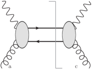
$=C_{u}\,\delta^{ac}\,h(Q,y,p_{T},y_{J},\mu)$

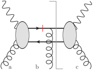
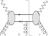
+ $=\left(C_{1}+C_{2}\right)\left(-if^{abc}\right)h(Q,y,p_{T},y_{J},\mu)$

Figure 2: Top: Unpolarized hard Feynman diagram for HF dijet production. Bottom: Polarized hard diagram for HF dijet production. The red lines in the polarized case indicate the location of a soft pole.

2.4 TMD PDFs and the global soft function

In order to regulate the rapidity divergences in the TMD PDFs and the global soft function, we use the $\eta$ regulator of Chiu:2012ir . The expression for the unsubtracted gluon TMD in this regularization scheme can be obtained from Kang:2017glf , and is given by

$$f_{g/g}^{\rm NLO}(x,b,\mu,\zeta/\nu^{2})=\delta(1-x)$$ (28)

$$\hskip 79.6678pt+\frac{\alpha_{s}}{4\pi}C_{A}\left[\frac{4}{\eta}\left(\frac{1}{\epsilon}+\ln\frac{\mu^{2}}{\mu_{b}^{2}}\right)+\frac{2}{\epsilon}\left(\ln\frac{\nu^{2}}{\left(n\cdot p_{g}\right)^{2}}+\frac{\beta_{0}}{C_{A}}\right)\right]\delta(1-x)$$

$$\hskip 79.6678pt-\frac{\alpha_{s}}{4\pi}\left[\frac{2}{\epsilon}+2\ln\frac{\mu^{2}}{\mu_{b}^{2}}\right]P_{gg}(x)$$

$$\hskip 79.6678pt+\frac{\alpha_{s}}{4\pi}C_{A}\left[\ln\frac{\mu^{2}}{\mu_{b}^{2}}\left(\ln\frac{\nu^{2}}{\left(n\cdot p_{g}\right)^{2}}+\frac{\beta_{0}}{C_{A}}\right)\delta(1-x)\right]\,,$$

$$f_{g/q}^{\rm NLO}(x,b,\mu,\zeta/\nu^{2})=-\frac{\alpha_{s}}{4\pi}\left[\frac{2}{\epsilon}+2\ln\frac{\mu^{2}}{\mu_{b}^{2}}\right]P_{gq}(x)+\frac{\alpha_{s}}{4\pi}C_{F}\left(2x\right)\,,$$ (29)

where we have set $\zeta=\left(n\cdot p_{g}\right)^{2}$ Ebert:2019okf , the scale $\mu_{b}$ is defined as $\mu_{b}=2e^{-\gamma_{E}}/b$, with $b$ being the magnitude of the two-dimensional vector transverse to the beam direction $\bm{b}=b\left(\cos\phi_{b},\sin\phi_{b}\right)$, and

$$P_{gg}(x)=2C_{A}\left[\frac{x}{(1-x)}_{+}+\frac{1-x}{x}+x(1-x)\right]+\frac{\beta_{0}}{2}\delta(1-x)\,,$$ (30)

$$P_{gq}(x)=C_{F}\frac{1+(1-x)^{2}}{x}\,,$$ (31)

are the collinear splitting kernels. The term in the third line of Eq. (28) and the analogous term in Eq. (29) contain the infrared divergences which are to be matched to the collinear PDF. The RG equations for the gluon TMD PDF are then

$$\frac{d}{d\ln\mu}\ln f_{g/N}(x,b,\mu,\zeta/\nu^{2})=\, \Gamma^{f_{g}}(\alpha_{s})\,,$$ (32)

$$\frac{d}{d\ln\nu}\ln f_{g/N}(x,b,\mu,\zeta/\nu^{2})=\, \gamma_{\nu}^{f_{g}}(\alpha_{s})\,.$$ (33)

Here the anomalous dimensions are given by

$$\Gamma^{f_{g}}(\alpha_{s})=C_{A}\gamma^{\textrm{cusp}}(\alpha_{s})\ln\frac{\nu^{2}}{(n\cdot p_{g})^{2}}-2\gamma^{f_{g}}(\alpha_{s})\,,\quad\gamma_{\nu}^{f_{g}}(\alpha_{s})=\frac{\alpha_{s}}{\pi}C_{A}\ln\frac{\mu^{2}}{\mu_{b}^{2}}+\mathcal{O}(\alpha_{s}^{2})\,,$$ (34)

with $\gamma^{f_{g}}_{0}=\gamma_{0}^{g}$, which is given in Eq. (2.3).

On the other hand, we define the soft function as

$$S^{\rm LO}(b,\mu,\nu) =1\,,$$ (35)

$$S^{\rm{NLO}}(\bm{b},\mu,\nu) =-\frac{C_{A}}{2}\,\mathcal{I}_{BJ}-\frac{C_{A}}{2}\,\mathcal{I}_{B\accentset{\rule{2.79996pt}{0.8pt}}{J}}+\left(\frac{C_{A}}{2}-C_{F}\right)\,\mathcal{I}_{J\accentset{\rule{2.79996pt}{0.8pt}}{J}}\,,$$ (36)

where the soft integrals $\mathcal{I}_{ij}$ are given by

$$\mathcal{I}_{ij}=\frac{\alpha_{s}\mu^{2\epsilon}\pi^{\epsilon}e^{\epsilon\gamma_{E}}}{\pi^{2}}\int d^{d}k\,\delta^{+}(k^{2})e^{-i\,k\cdot b}\frac{n_{i}\cdot n_{j}}{(n_{i}\cdot k)(n_{j}\cdot k)}\frac{\nu^{\eta}}{|k^{+}-k^{-}|^{\eta}}\,.$$ (37)

Here, $i$ and $j$ are either $B$, $J$, or $\accentset{\rule{2.79996pt}{0.8pt}}{J}$, where $B$ denotes the beam direction while $J$ and $\accentset{\rule{2.79996pt}{0.8pt}}{J}$ denote the directions of the jet initiated by the HF quark and anti-quark, respectively. The expressions for the $\phi_{b}$-dependent beam-jet soft function integrals are given in Buffing:2018ggv as

$$\mathcal{I}_{BJ}= \,\frac{\alpha_{s}}{4\pi}\Bigg{[}\frac{4}{\eta}\left(\frac{1}{\epsilon}+\ln\frac{\mu^{2}}{\mu_{b}^{2}}\right)-\frac{4}{\epsilon^{2}}-\frac{2}{\epsilon}\left(-2y_{J}-\ln\frac{\nu^{2}}{\mu^{2}}+2\ln\frac{2i\mu\,c_{bJ}}{\mu_{b}}\right)\Bigg{]}+\mathcal{I}_{BJ}^{\textrm{fin}},$$ (38)

$$\mathcal{I}_{B\accentset{\rule{2.79996pt}{0.8pt}}{J}}= \,\frac{\alpha_{s}}{4\pi}\Bigg{[}\frac{4}{\eta}\left(\frac{1}{\epsilon}+\ln\frac{\mu^{2}}{\mu_{b}^{2}}\right)-\frac{4}{\epsilon^{2}}-\frac{2}{\epsilon}\left(-2y_{\accentset{\rule{2.79996pt}{0.8pt}}{J}}-\ln\frac{\nu^{2}}{\mu^{2}}+2\ln\frac{-2i\mu\,c_{bJ}}{\mu_{b}}\right)\Bigg{]}+\mathcal{I}_{B\accentset{\rule{2.79996pt}{0.8pt}}{J}}^{\textrm{fin}},$$ (39)

with $c_{bJ}=\cos(\phi_{b}-\phi_{J})$ and where the rapidity of jets are

$$y_{J}=\ln\frac{zQ}{p_{T}},\qquad y_{\accentset{\rule{2.79996pt}{0.8pt}}{J}}=\ln\frac{(1-z)Q}{p_{T}}\,.$$ (40)

Here, the terms marked by “fin” in their superscripts denote the finite contributions of their respective functions. While the divergent pieces are required for the purposes of resummation, the finite pieces are only needed at NLO. Since we perform our analysis at NLL accuracy, these terms are not needed for this study. Recently in delCastillo:2020omr , the authors derive the following the jet-jet soft function integral which contains no rapidity divergence. This integral can be written as

$$\mathcal{I}_{J\accentset{\rule{2.79996pt}{0.8pt}}{J}}=\frac{\alpha_{s}}{4\pi}\left[-\frac{4}{\epsilon^{2}}+\frac{4}{\epsilon}\left(\ln\frac{\hat{s}}{p_{T}^{2}}-\ln\frac{\mu^{2}}{\mu_{b}^{2}}-\ln\left(4c_{bJ}^{2}\right)\right)\right]+\mathcal{I}_{J\accentset{\rule{2.79996pt}{0.8pt}}{J}}^{\textrm{fin}}\,.$$ (41)

From Eqs. (38), (39), and (41), we obtain the following expressions for the soft anomalous dimensions

$$\Gamma^{s}(\alpha_{s}) =2C_{F}\,\gamma^{\rm{cusp}}(\alpha_{s})\ln\frac{\mu^{2}}{\mu_{b}^{2}}-C_{A}\,\gamma^{\rm{cusp}}(\alpha_{s})\ln\frac{\nu^{2}}{\mu^{2}}+\gamma^{s}(\alpha_{s})\,,$$ (42)

$$\gamma_{\nu}^{s}(\alpha_{s}) =-\frac{\alpha_{s}}{\pi}C_{A}\ln\frac{\mu^{2}}{\mu_{b}^{2}}+\mathcal{O}(\alpha_{s}^{2})\,,$$ (43)

with the one-loop single logarithmic anomalous dimension

$$\gamma_{0}^{s}=8C_{F}\ln\left(4c_{bJ}^{2}\right)+4(C_{A}-2C_{F})\ln\frac{\hat{s}}{p_{T}^{2}}+4\,C_{A}\ln\frac{\hat{s}}{Q^{2}}\,.$$ (44)

As expected, we see that the one-loop rapidity anomalous dimensions of the TMD PDF and the soft function fulfill the condition

$$\gamma_{\nu,0}^{f_{g}}+\gamma_{\nu,0}^{s}=0\,.$$ (45)

Thus, the product of $f_{g/N}(x,b,\mu,\zeta/\nu^{2})$ and $S(\bm{b},\mu,\nu)$ is $\nu$-independent, and we can construct the properly-defined gluon TMD PDF as in Eq. (11).

Here we find that the soft function depends not only the magnitude but also the direction of the vector $\bm{b}$. As shown in Sec. 2.6 a similar structure also shows up in the collinear-soft function, and the $\phi_{b}$ dependence in the anomalous dimensions will cancel out between these two functions. However, after taking into account the evolution between the soft and collinear-soft function, one finds that the $\phi_{b}$ integral is divergent in some phase space region. In order to avoid such divergences we apply methods in Buffing:2018ggv ; Kang:2020xez where one first performs an averaging over the $\phi_{b}$ angle in both soft and collinear-soft function. We note that this method does not change the RG invariance as shown in Eqs. (73) and (74). In addition, as discussed in Chien:2019gyf no significant numerical effects between different methods are observed in the NLL resummation calculation.

The $\phi_{b}$-averaged soft function can be constructed from Eqs. (35) and (36) by replacing the soft integrals with

$$\bar{\mathcal{I}}_{BJ}=\frac{\alpha_{s}}{4\pi} \left[2\left(\frac{2}{\eta}+\ln\frac{\nu^{2}}{\mu^{2}}+2y_{J}\right)\left(\frac{1}{\epsilon}+\ln\frac{\mu^{2}}{\mu_{b}^{2}}\right)-\frac{4}{\epsilon^{2}}-\frac{2}{\epsilon}\ln\frac{\mu^{2}}{\mu_{b}^{2}}+\frac{\pi^{2}}{3}\right]\,,$$ (46)

$$\bar{\mathcal{I}}_{B\accentset{\rule{2.79996pt}{0.8pt}}{J}}=\frac{\alpha_{s}}{4\pi} \left[2\left(\frac{2}{\eta}+\ln\frac{\nu^{2}}{\mu^{2}}+2y_{\accentset{\rule{2.79996pt}{0.8pt}}{J}}\right)\left(\frac{1}{\epsilon}+\ln\frac{\mu^{2}}{\mu_{b}^{2}}\right)-\frac{4}{\epsilon^{2}}-\frac{2}{\epsilon}\ln\frac{\mu^{2}}{\mu_{b}^{2}}+\frac{\pi^{2}}{3}\right]\,,$$ (47)

$$\bar{\mathcal{I}}_{J\accentset{\rule{2.79996pt}{0.8pt}}{J}}=\frac{\alpha_{s}}{2\pi} \,\bigg{[}4\left(\frac{1}{\epsilon}+\ln\frac{\mu^{2}}{\mu_{b}^{2}}\right)\ln\big{(}2\cosh(\Delta y/2)\big{)}-\frac{2}{\epsilon^{2}}-\frac{2}{\epsilon}\ln\frac{\mu^{2}}{\mu_{b}^{2}}-\ln^{2}\frac{\mu^{2}}{\mu_{b}^{2}}+\Delta y^{2}$$

$$-4\ln^{2}\big{(}2\cosh(\Delta y/2)\big{)}+\frac{\pi^{2}}{6}\bigg{]}\,,$$ (48)

where we have placed a bar over these integrals in order to distinguish them from the $\phi_{b}$-dependent ones and have defined $\Delta y=y_{J}-y_{\accentset{\rule{2.79996pt}{0.8pt}}{J}}$. These results are the same as the soft function calculated in Hornig:2017pud . Therefore, the anomalous dimensions for the averaged case are

$$\bar{\Gamma}^{s}(\alpha_{s}) =2C_{F}\,\gamma^{\rm{cusp}}(\alpha_{s})\ln\frac{\mu^{2}}{\mu_{b}^{2}}-C_{A}\,\gamma^{\rm{cusp}}(\alpha_{s})\ln\frac{\nu^{2}}{\mu^{2}}+\bar{\gamma}^{s}(\alpha_{s})\,,$$ (49)

$$\bar{\gamma}_{\nu}^{s}(\alpha_{s}) =-\frac{\alpha_{s}}{\pi}C_{A}\ln\frac{\mu^{2}}{\mu_{b}^{2}}+\mathcal{O}(\alpha_{s}^{2})\,,$$ (50)

where the one-loop single logarithmic anomalous dimensions is

$$\bar{\gamma}_{0}^{s}=4(C_{A}-2C_{F})\ln\frac{\hat{s}}{p_{T}^{2}}+4C_{A}\ln\frac{\hat{s}}{Q^{2}}\,.$$ (51)

By comparing Eqs. (43) and (50), one can see the rapidity anomalous dimension is unchanged. Therefore in the $\phi_{b}$-averaged case, we can once again write the factorized expression in terms of the properly defined TMD PDFs.

2.5 Massive quark jet function

In this section, we discuss the calculation of the massive quark jet function at NLO. The massive quark jet function has been investigated in detail for various observables. For example, the factorization formula for the massive event shape distribution involves such a jet function, as the jet and heavy quark masses are of similar magnitude Fleming:2007qr ; Fleming:2007xt ; Lepenik:2019jjk ; Bris:2020uyb . The corresponding jet function has been calculated to two-loop order Hoang:2019fze . Furthermore, the semi-inclusive massive quark jet fragmentation function has been calculated at NLO and applied to inclusive jet production Dai:2018ywt ; Li:2018xuv . Recently, the one-loop expression for the so-called unmeasured massive quark jet function has been presented in Kim:2020dgu .

The global jet anomalous dimension can be obtained from the divergent terms of the unmeasured massive quark jet function. As shown in Fig. 3, the one-loop calculation involves two types of diagrams: $J_{\mathcal{Q}}^{\rm NLO,V}$ and $J_{\mathcal{Q}}^{\rm NLO,R}$, where $J_{\mathcal{Q}}^{\rm NLO,V}$ contains only single cut propagators and is thereby unconstrained by the jet algorithm. Explicitly, it is written as

$$J_{\mathcal{Q}}^{\rm NLO,V}=\frac{\alpha_{s}}{4\pi}C_{F}\left[\frac{2}{\epsilon^{2}}+\frac{1}{\epsilon}\left(1+2\ln\frac{\mu^{2}}{m_{\mathcal{Q}}^{2}}\right)+\left(1+\ln\frac{\mu^{2}}{m_{\mathcal{Q}}^{2}}\right)\ln\frac{\mu^{2}}{m_{\mathcal{Q}}^{2}}+4+\frac{\pi^{2}}{6}\right]\,,$$ (52)

where the heavy quark mass $m_{\mathcal{Q}}$ is the only physical scale involved. Since the real contribution $J_{\mathcal{Q}}^{\rm NLO,R}$ is constrained by the jet algorithm, it will depend on the jet scale $p_{T}R$ in addition to $m_{\mathcal{Q}}$. In this work, we define the HF quark four-momentum $q^{\mu}$ with $q^{2}=m_{\mathcal{Q}}^{2}$, which is known as the M-scheme Bris:2020uyb . We note that in the hierarchy of scales we are considering, the constraint of the anti-$k_{T}$ algorithm Cacciari:2008gp is independent of the HF quark mass $m_{\mathcal{Q}}$ and is in fact identical to that for massless partons Dai:2018ywt , namely

$$\Theta_{\operatorname{anti-}\!k_{T}}=\theta\left[\left(\frac{q^{-}\left(\omega_{J}-q^{-}\right)}{\omega_{J}}\right)^{2}\left(\frac{R}{2\,\mathrm{cosh}\,y_{J}}\right)^{2}-\bm{q}_{\perp}^{2}\right]\,,$$ (53)

where $q^{\mu}=(q^{+},q^{-},\bm{q}_{\perp})$ is the four-momentum of the HF quark and $\omega_{J}$ is the large component of the jet four-momentum. The jet scale $p_{T}R$ emerges in Eq. (53) upon noting $\omega_{J}=2\,p_{T}\,\mathrm{cosh}\,y_{J}$. In the phase space integral, we expand the integrated momentum $q$ along the jet direction with $q^{+}=(m_{\mathcal{Q}}^{2}+\bm{q}_{\perp}^{2})/q^{-}$ given by the power counting requirement $p_{T}R\sim m_{\mathcal{Q}}$. Explicitly, we have

$$J_{\mathcal{Q}}^{\rm NLO,R}(p_{T}R,m_{\mathcal{Q}}, \epsilon)=\frac{\alpha_{s}C_{F}e^{\epsilon\gamma_{E}}\mu^{2\epsilon}}{2\pi\Gamma(1-\epsilon)}\int\frac{dq^{-}}{\omega_{J}}\frac{d\bm{q}_{\perp}^{2}}{\bm{q}_{\perp}^{2\epsilon}}\Bigg{[}\frac{q^{-}}{\omega_{J}-q^{-}}\frac{2\bm{q}_{\perp}^{2}\omega_{J}^{4}}{[\bm{q}_{\perp}^{2}\omega_{J}^{2}+m_{\mathcal{Q}}^{2}(\omega_{J}-q^{-})^{2}]^{2}}$$

$$+(1-\epsilon)\frac{\omega_{J}(\omega_{J}-q^{-})}{\bm{q}_{\perp}^{2}\omega_{J}^{2}+m_{\mathcal{Q}}^{2}(\omega_{J}-q^{-})^{2}}\Bigg{]}\theta(\omega_{J}-q^{-})\Theta_{\operatorname{anti-}\!k_{T}}$$

$$=\frac{\alpha_{s}}{4\pi}C_{F}\left[-2\ln\left(\frac{m_{\mathcal{Q}}^{2}+p_{T}^{2}R^{2}}{m_{\mathcal{Q}}^{2}}\right)+2-\frac{2m_{\mathcal{Q}}^{2}}{m_{\mathcal{Q}}^{2}+p_{T}^{2}R^{2}}\right]\frac{1}{\epsilon}+J_{\mathcal{Q}}^{\mathrm{R,fin}}\,,$$ (54)

where only a single divergence is exhibited, as the heavy quark mass $m_{\mathcal{Q}}$ acts as a regulator of the overlapping soft and collinear regions of phase space. After combining the real and virtual contributions, the logarithmic dependence on the quark mass $m_{\mathcal{Q}}$ cancels out.

\begin{overpic}[width=368.57964pt]{jetfun} \color[rgb]{0,0,0}\put(310.0,20.0){$q$} \end{overpic}

Figure 3: Sample Feynman diagrams contributing to the massive quark jet function $J_{\mathcal{Q}}$ at one-loop order in perturbation theory. The virtual corrections $J_{\mathcal{Q}}^{\rm NLO,V}$ are displayed in the first two diagrams, where each contain only a single cut propagator. The remaining diagrams involving two cut propagators represent the real corrections $J_{\mathcal{Q}}^{\rm NLO,R}$.

The one-loop global jet renormalization constant then reads

$$Z^{J_{\mathcal{Q}}}=1+\frac{\alpha_{s}}{4\pi}C_{F}\left[\frac{2}{\epsilon^{2}}+\frac{1}{\epsilon}\left(2\ln\frac{\mu^{2}}{m_{\mathcal{Q}}^{2}+p_{T}^{2}R^{2}}+3-\frac{2m_{\mathcal{Q}}^{2}}{m_{\mathcal{Q}}^{2}+p_{T}^{2}R^{2}}\right)\right]\,,$$ (55)

where, again, we observe that the heavy quark mass $m_{\mathcal{Q}}$ only affects the single pole structure. We further note that as $m_{\mathcal{Q}}\to 0$, the massive quark jet renormalization constant reduces to that of the massless jet, $Z^{J_{\mathcal{Q}}}\to Z^{J_{q}}$. This gives us the following expression for the global jet anomalous dimension

$$\Gamma^{j_{\mathcal{Q}}}(\alpha_{s})=-C_{F}\gamma^{\rm cusp}(\alpha_{s})\ln\frac{m_{\mathcal{Q}}^{2}+p_{T}^{2}R^{2}}{\mu^{2}}+\gamma^{j_{\mathcal{Q}}}(\alpha_{s})\,,$$ (56)

with the one-loop single logarithmic anomalous dimension as

$$\gamma_{0}^{j_{\mathcal{Q}}}=2C_{F}\left(3-\frac{2m_{\mathcal{Q}}^{2}}{m_{\mathcal{Q}}^{2}+p_{T}^{2}R^{2}}\right)\,,$$ (57)

where the first term in the brackets is shared by the massless quark jet function and the second term constitutes the finite quark mass correction. Finally, the renormalized HF jet function is given by the following

$$J_{\mathcal{Q},{\rm NLO}}^{\mathrm{ren.}}(p_{T}R,m_{\mathcal{Q}},\mu)= \,\frac{\alpha_{s}}{4\pi}C_{F}\Bigg{[}\left(3-\frac{2m_{\mathcal{Q}}^{2}}{m_{\mathcal{Q}}^{2}+p_{T}^{2}R^{2}}\right)\ln\frac{\mu^{2}}{m_{\mathcal{Q}}^{2}+p_{T}^{2}R^{2}}$$ (58)

$$\hskip 71.13188pt+\ln^{2}\frac{\mu^{2}}{m_{\mathcal{Q}}^{2}+p_{T}^{2}R^{2}}+13-\frac{3\pi^{2}}{2}+\mathcal{F}(p_{T}R,m_{\mathcal{Q}})\Bigg{]}\,,$$

where the function $\mathcal{F}(p_{T}R,m_{\mathcal{Q}})$ can be expressed as

$$\mathcal{F}(p_{T}R,m_{\mathcal{Q}})= \,\pi^{2}-4\,\mathrm{Li}_{2}\left(-\frac{m_{\mathcal{Q}}^{2}}{p_{T}^{2}R^{2}}\right)+2\left(1-\ln\frac{m_{\mathcal{Q}}^{2}}{p_{T}^{2}R^{2}}\right)\ln\frac{m_{\mathcal{Q}}^{2}+p_{T}^{2}R^{2}}{p_{T}^{2}R^{2}}$$

$$-\frac{2m_{\mathcal{Q}}^{2}}{m_{\mathcal{Q}}^{2}+p_{T}^{2}R^{2}}\ln\frac{m_{\mathcal{Q}}^{2}}{p_{T}^{2}R^{2}}-\frac{m_{\mathcal{Q}}^{2}}{p_{T}^{2}R^{2}}\ln\frac{m_{\mathcal{Q}}^{2}+p_{T}^{2}R^{2}}{m_{\mathcal{Q}}^{2}}$$

$$-4\bigg{[}\frac{m_{\mathcal{Q}}}{p_{T}R}\left(1+\frac{m_{\mathcal{Q}}^{2}}{m_{\mathcal{Q}}^{2}+p_{T}^{2}R^{2}}\right)+\mathrm{Cot}^{-1}\left(\frac{m_{\mathcal{Q}}}{p_{T}R}\right)\bigg{]}\mathrm{Cot}^{-1}\left(\frac{m_{\mathcal{Q}}}{p_{T}R}\right)\,.$$ (59)

This expression for the HF jet function is equivalent to the semi-analytic form presented in Kim:2020dgu , and one can see that as $m_{\mathcal{Q}}\rightarrow 0$, we have $\mathcal{F}\rightarrow 0$ and, therefore, $J_{\mathcal{Q}}\rightarrow J_{q}$. Hence, the massive quark jet function behaves as expected in the massless limit.

2.6 Collinear-soft function

In this section, we calculate the one-loop perturbative expression for the collinear-soft function $S^{c}_{\mathcal{Q}}(\bm{b},R,m_{\mathcal{Q}},\mu)$. The corresponding Feynman diagrams are shown in Fig. 4, where the blue and black lines represent Wilson lines along $v_{J}^{\mu}$ and $\bar{n}_{J}^{\mu}$ directions, respectively. Here, the massive quark velocity $v_{J}^{\mu}$ is defined by

$$v_{J}^{\mu}=\frac{\omega_{J}}{m_{\mathcal{Q}}}\frac{n_{J}^{\mu}}{2}+\frac{m_{\mathcal{Q}}}{\omega_{J}}\frac{\bar{n}_{J}^{\mu}}{2}\,,\quad\quad{\rm with}~{}v_{J}^{2}=1\,.$$ (60)

Explicitly, the bare NLO collinear-soft function is given by

$$S_{\mathcal{Q},{\rm NLO}}^{c}(\bm{b},R,m_{\mathcal{Q}},\epsilon)=2C_{F}\,w_{\bar{n}_{J}v_{J}}-C_{F}\,w_{v_{J}v_{J}}\,,$$ (61)

where the collinear-soft integrals $w_{\alpha\beta}$ are defined in $b$-space as

$$w_{\alpha\beta}=\frac{\alpha_{s}\mu^{2\epsilon}\pi^{\epsilon}e^{\epsilon\gamma_{E}}}{2\pi^{2}}\int d^{d}k\,\delta^{+}(k^{2})e^{-i\,\bar{n}_{J}\cdot k\,n_{J}\cdot b/2}\frac{\alpha\cdot\beta}{\left(\alpha\cdot k\right)\left(\beta\cdot k\right)}\,\theta\left[\frac{n_{J}\cdot k}{\bar{n}_{J}\cdot k}-\left(\frac{R}{2\cosh y_{J}}\right)^{2}\right]\,.$$ (62)

Upon performing the $k$-integration, we obtain the following expressions for $w_{\alpha\beta}$

\begin{overpic}[width=325.215pt]{coft.eps} \color[rgb]{0,0,1}\put(10.0,74.0){$v_{J}^{\mu}$} \color[rgb]{0,0,0}\put(8.0,8.0){$\bar{n}_{J}^{\mu}$} \end{overpic}

Figure 4: One-loop Feynman diagrams of the collinear-soft function $S^{c}_{\mathcal{Q}}$. The blue and black lines indicate the Wilson lines along $v_{J}^{\mu}$ and $\bar{n}_{J}^{\mu}$ directions, respectively.

$$w_{\bar{n}_{J}v_{J}}= \frac{\alpha_{s}}{4\pi}\left[-\frac{1}{\epsilon^{2}}-\frac{1}{\epsilon}\left(\ln\frac{\mu^{2}}{\mu_{b}^{2}}+2\ln\frac{-2ic_{bJ}}{R}-\ln\frac{m_{\mathcal{Q}}^{2}+p_{T}^{2}R^{2}}{p_{T}^{2}R^{2}}\right)\right]+w_{\bar{n}_{J}v_{J}}^{\mathrm{fin}}\,,$$ (63)

$$w_{v_{J}v_{J}}= \frac{\alpha_{s}}{4\pi}\left[-\frac{1}{\epsilon}\left(\frac{2m_{\mathcal{Q}}^{2}}{m_{\mathcal{Q}}^{2}+p_{T}^{2}R^{2}}\right)\right]+w_{v_{J}v_{J}}^{\mathrm{fin}}\,.$$ (64)

We see that the finite quark mass corrections only enter into the single pole structure of the collinear-soft function. This is analogous to the observation made in Sec. 2.5 in analyzing the massive quark jet function, and can be understood through the same physical reasoning. The finite terms are given by

$$w_{\bar{n}_{J}v_{J}}^{\mathrm{fin}} =\frac{\alpha_{s}}{4\pi}\Biggl{[}2\left(\ln\frac{m_{\mathcal{Q}}^{2}+p_{T}^{2}R^{2}}{p_{T}^{2}R^{2}}-\ln\frac{-2i\,c_{bJ}}{R}\right)\ln\frac{-2i\,c_{bJ}}{R}$$ (65)

$$+\left(\ln\frac{m_{\mathcal{Q}}^{2}+p_{T}^{2}R^{2}}{p_{T}^{2}R^{2}}-2\ln\frac{-2i\,c_{bJ}}{R}-\frac{1}{2}\ln\frac{\mu^{2}}{\mu_{b}^{2}}\right)\ln\frac{\mu^{2}}{\mu_{b}^{2}}+\mathrm{Li}_{2}\left(-\frac{m_{\mathcal{Q}}^{2}}{p_{T}^{2}R^{2}}\right)-\frac{\pi^{2}}{4}\Biggr{]}\,,$$

$$w_{v_{J}v_{J}}^{\mathrm{fin}} =\frac{\alpha_{s}}{4\pi}\left[2\ln\frac{m_{\mathcal{Q}}^{2}+p_{T}^{2}R^{2}}{p_{T}^{2}R^{2}}-\frac{2m_{\mathcal{Q}}^{2}}{m_{\mathcal{Q}}^{2}+p_{T}^{2}R^{2}}\left(2\ln\frac{-2i\,c_{bJ}}{R}+\ln\frac{\mu^{2}}{\mu_{b}^{2}}\right)\right]\,.$$ (66)

Here, we note that $w_{\bar{n}_{J}v_{J}}$ reduces to the massless $w_{\bar{n}_{J}n_{J}}$ function Buffing:2018ggv ; Chien:2019gyf as $m_{\mathcal{Q}}\to 0$, while $w_{v_{J}v_{J}}$ vanishes. Given the expression for $S_{\mathcal{Q}}^{c}$, we can calculate the renormalization constant $Z^{S_{\mathcal{Q}}^{c}}$, which is given by

$$Z^{S_{\mathcal{Q}}^{c}} =1$$ (67)

$$+\frac{\alpha_{s}}{4\pi}C_{F}\left[-\frac{2}{\epsilon^{2}}-\frac{2}{\epsilon}\left(\ln\frac{\mu^{2}}{\mu_{b}^{2}}+2\ln\frac{-2ic_{bJ}}{R}-\frac{m_{\mathcal{Q}}^{2}}{m_{\mathcal{Q}}^{2}+p_{T}^{2}R^{2}}-\ln\frac{m_{\mathcal{Q}}^{2}+p_{T}^{2}R^{2}}{p_{T}^{2}R^{2}}\right)\right]\,.$$

This renormalization constant leads to the following formula for global collinear-soft anomalous dimension

$$\Gamma^{cs_{\mathcal{Q}}}(\alpha_{s})=C_{F}\gamma^{\rm cusp}(\alpha_{s})\ln\frac{R^{2}\mu_{b}^{2}}{\mu^{2}}+\gamma^{cs_{\mathcal{Q}}}(\alpha_{s})\,,$$ (68)

where the one-loop single logarithmic anomalous dimension is

$$\gamma_{0}^{cs_{\mathcal{Q}}}=-4C_{F}\left[2\ln\left(-2ic_{bJ}\right)-\frac{m_{\mathcal{Q}}^{2}}{m_{\mathcal{Q}}^{2}+p_{T}^{2}R^{2}}-\ln\frac{m_{\mathcal{Q}}^{2}+p_{T}^{2}R^{2}}{p_{T}^{2}R^{2}}\right]\,.$$ (69)

The anomalous dimension for the collinear-soft function associated with the anti-quark is given by

$$\Gamma^{cs_{\bar{\mathcal{Q}}}}(\alpha_{s})=\Gamma^{cs_{\mathcal{Q}}}(\alpha_{s})|_{\phi_{J}\rightarrow\phi_{J}+\pi}\,.$$ (70)

For phenomenological purposes, we utilize the $\phi_{b}$-averaged collinear-soft function, which can be obtained through Eq. (63) by making use of the following integrals

$$\int_{0}^{2\pi}\frac{d\phi_{b}}{2\pi}\ln\left(-2ic_{bJ}\right)=0\,,\qquad\int_{0}^{2\pi}\frac{d\phi_{b}}{2\pi}\ln^{2}\left(-2ic_{bJ}\right)=-\frac{\pi^{2}}{6}\,.$$ (71)

The resulting anomalous dimension for the $\phi_{b}$-averaged collinear-soft function is denoted by $\bar{\Gamma}^{cs_{\mathcal{Q}}}$ with

$$\bar{\gamma}_{0}^{cs_{\mathcal{Q}}}=4C_{F}\left(\frac{m_{\mathcal{Q}}^{2}}{m_{\mathcal{Q}}^{2}+p_{T}^{2}R^{2}}+\ln\frac{m_{\mathcal{Q}}^{2}+p_{T}^{2}R^{2}}{p_{T}^{2}R^{2}}\right)\,.$$ (72)

Upon integrating over $\phi_{b}$, we find that $\bar{\Gamma}^{cs_{\bar{\mathcal{Q}}}}(\alpha_{s})=\bar{\Gamma}^{cs_{\mathcal{Q}}}(\alpha_{s})$ and, therefore, the two averaged collinear-soft functions $\bar{S}_{\mathcal{Q}}^{c}$ and $\bar{S}_{\bar{\mathcal{Q}}}^{c}$ behave identically under QCD evolution.

2.7 Renormalization group consistency

Armed with the anomalous dimensions of each component, we are now positioned to demonstrate the RG consistency of our factorization framework.

Inspection of Eqs. (56) and (68) reveals that all mass corrections cancel exactly in the sum $\Gamma^{j_{\mathcal{Q}}}+\Gamma^{cs_{\mathcal{Q}}}$, making the RG consistency of our formalism identical to the massless case. A similar observation is made in Kim:2020dgu . This general physical behavior has also been observed in the context of inclusive HF jet production Dai:2018ywt , where the authors offer the intuitive argument that as the heavy quark mass $m_{\mathcal{Q}}$ constitutes IR information, it thus does not affect the UV behavior of the semi-inclusive jet function. In the present context, we see that the UV evolution behavior of the product of the jet and collinear-soft functions is insensitive to the IR scale introduced by the heavy quark mass. However, in Sec. 2.8, we will see how the heavy quark mass enters non-trivially and crucially into the evaluation of the differential cross section.

Therefore, upon combining Eqs. (22), (34), (42), (55) and (68), the RG consistency of our formalism is established:

$$\Gamma^{h}+\Gamma^{s}+\Gamma^{f_{g}}+2\Gamma^{j_{\mathcal{Q}}}+\Gamma^{cs_{\mathcal{Q}}}+\Gamma^{cs_{\bar{\mathcal{Q}}}}=0\,.$$ (73)

Furthermore, we note that this consistency is preserved under the operation of $\phi_{b}$-averaging

$$\Gamma^{h}+\bar{\Gamma}^{s}+\Gamma^{f_{g}}+2\Gamma^{j_{\mathcal{Q}}}+\bar{\Gamma}^{cs_{\mathcal{Q}}}+\bar{\Gamma}^{cs_{\bar{\mathcal{Q}}}}=0\,.$$ (74)

2.8 Resummation formula

Utilizing our EFT framework, all-order resummation is achieved through RG evolution. The resulting all-order expression for the HF dijet production cross section is given at NLL by

$$\frac{d\sigma^{UU}}{dQ^{2}dyd^{2}\bm{q}_{T}dy_{J}d^{2}\bm{p}_{T}}=H(Q,y,p_{T},y_{J},\mu_{h})\int_{0}^{\infty}\frac{bdb}{2\pi}J_{0}(b\,q_{T})f_{g/N}(x,\mu_{b*})$$

$$\hskip 18.06749pt\times\exp\left[-\int_{\mu_{b*}}^{\mu_{h}}\frac{d\mu}{\mu}\Gamma^{h}\left(\alpha_{s}\right)-2\int_{\mu_{b*}}^{\mu_{j}}\frac{d\mu}{\mu}\Gamma^{j_{\mathcal{Q}}}\left(\alpha_{s}\right)-\int_{\mu_{b_{*}}}^{\mu_{cs}}\frac{d\mu}{\mu}\left(\bar{\Gamma}^{cs_{\mathcal{Q}}}\left(\alpha_{s}\right)+\bar{\Gamma}^{cs_{\bar{\mathcal{Q}}}}\left(\alpha_{s}\right)\right)\right]$$

$$\hskip 18.06749pt\times\exp\left[-S_{\rm NP}(b,Q_{0},n\cdot p_{g})\right]\,,$$ (75)

where $J_{0}$ is the zeroth order Bessel function of the first kind. In this expression, $\mu_{h}$, $\mu_{j}$, and $\mu_{cs}$ are the hard, jet, and collinear-soft scales, respectively. We have also performed the usual operator product expansion (OPE) of the unpolarized gluon TMD PDF $f_{g/N}(x,b,\mu,\zeta)$ in terms of the collinear gluon PDF $f_{g/N}(x,\mu)$ at the initial scales $\zeta_{i}=\mu_{i}^{2}=\mu_{b*}^{2}$, and have kept the coefficient at LO to be consistent with NLL accuracy. The matching coefficient at higher-orders can be found in e.g. Echevarria:2015uaa ; Catani:2011kr ; Gehrmann:2014yya ; Luebbert:2016itl ; Echevarria:2016scs ; Luo:2019bmw ; Ebert:2020yqt . The function $S_{\rm NP}$ parameterizes the contribution from non-perturbative power corrections which are enhanced for $q_{T}\sim\Lambda_{\rm QCD}$. Explicitly, we apply the formula given in Su:2014wpa , which reads

$$S_{\mathrm{NP}}\left(b,Q_{0},n\cdot p_{g}\right)=g_{1}b^{2}+\frac{g_{2}}{2}\frac{C_{A}}{C_{F}}\ln\frac{n\cdot p_{g}}{Q_{0}}\ln\frac{b}{b_{*}}\,.$$ (76)

We assign the following values to the parameters: $g_{1}=0.106\,\mathrm{GeV}^{2}$, $g_{2}=0.84$ and $Q_{0}^{2}=2.4\,\mathrm{GeV}^{2}$, and use the standard $b_{*}$-prescription Collins:1984kg

$$b_{*}=\frac{b}{\sqrt{1+b^{2}/b_{\rm max}^{2}}},\quad\qquad{\rm with}~{}~{}b_{\rm max}=1.5{\rm~{}GeV}^{-1}$$ (77)

in order to regularize the Landau singularity as $b\to\infty$.

Moreover, the spin-dependent cross section is expressed as

$$\frac{d\sigma^{UT}(\bm{S}_{T})}{dQ^{2}dyd^{2}\bm{q}_{T}dy_{J}d^{2}\bm{p}_{T}}=\sin(\phi_{q}-\phi_{s})\,H(Q,y,p_{T},y_{J},\mu_{h})\,\int_{0}^{\infty}\frac{b^{2}db}{4\pi}J_{1}(b\,q_{T})f_{1T,g/N}^{\perp,f}(x,\mu_{b*})$$

$$\hskip 18.06749pt\times\exp\left[-\int_{\mu_{b*}}^{\mu_{h}}\frac{d\mu}{\mu}\Gamma^{h}\left(\alpha_{s}\right)-2\int_{\mu_{b*}}^{\mu_{j}}\frac{d\mu}{\mu}\Gamma^{j_{\mathcal{Q}}}\left(\alpha_{s}\right)-\int_{\mu_{b_{*}}}^{\mu_{cs}}\frac{d\mu}{\mu}\left(\bar{\Gamma}^{cs_{\mathcal{Q}}}\left(\alpha_{s}\right)+\bar{\Gamma}^{cs_{\bar{\mathcal{Q}}}}\left(\alpha_{s}\right)\right)\right]$$

$$\hskip 18.06749pt\times\exp\left[-S^{\perp}_{\rm NP}(b,Q_{0},n\cdot p_{g})\right]\,.$$ (78)

Here, we have expected a similar OPE for the gluon Sivers function $f_{1T,g/N}^{\perp}(x,b,\mu,\zeta)$ at the initial scales $\zeta_{i}=\mu_{i}^{2}=\mu_{b*}^{2}$ and simply expressed the corresponding collinear function at LO as $f_{1T,g/N}^{\perp,f}(x,\mu_{b*})$ for simplicity. In principle, the corresponding collinear functions in the OPE expansion would be the twist-3 three-gluon correlation functions defined in Ji:1992eu ; Beppu:2010qn . To the best of our knowledge, detailed OPE calculations for the corresponding coefficient functions are not available in the literature. An expansion of the gluon Sivers function in terms of the collinear twist-3 quark-gluon-quark correlator, or the so-called Qiu-Sterman function Qiu:1991pp ; Qiu:1991wg , in transverse momentum space is performed in Yuan:2008vn . On the other hand, the coefficient functions for the expansion of the quark Sivers function in terms of the three-gluon correlation functions are provided in Dai:2014ala ; Scimemi:2019gge . The computation of the coefficient functions for expanding the gluon Sivers function in terms of the three-gluon correlation functions is essential for a full understanding of the QCD evolution of the gluon Sivers function. We leave this to future work.

Our knowledge about gluon Sivers functions, especially in the proper TMD factorization formalism, is rather limited. At the present moment, the only experimental constraint on the gluon Sivers function, in the TMD framework, comes from the SIDIS measurement of back-to-back hadron pairs off transversely-polarized deuterons and protons at COMPASS Adolph:2017pgv . However, as of yet, there has been no theoretical extraction of the gluon Sivers function from such data. On the other hand, an important theoretical constraint on the gluon Sivers function comes from the Burkardt sum rule Burkardt:2004ur . For the phenomenological purposes of the next section, we adopt the non-perturbative parameterization utilized by DAlesio:2015fwo ; Aschenauer:2015ndk  . Specifically, for the non-perturbative Sudakov, we take

$$S_{\mathrm{NP}}^{\perp}\left(b,Q_{0},n\cdot p_{g}\right)=g_{1}\rho\,b^{2}+\frac{g_{2}}{2}\frac{C_{A}}{C_{F}}\ln\frac{n\cdot p_{g}}{Q_{0}}\ln\frac{b}{b_{*}}\,,$$ (79)

where the $g_{2}$-dependent term is spin-independent and is, therefore, the same term occurring in Eq. (76), while the term $\propto g_{1}\rho$ can be connected to the Gaussian width in transverse momentum space Echevarria:2014xaa for the gluon Sivers function. For the collinear part of the gluon Sivers function, $f_{1T,g/p}^{\perp,f}(x,\mu)$ in Eq. (2.8), we take

$$f_{1T,g/N}^{\perp f}(x,\mu)=N_{g}\frac{4\rho\sqrt{2e\rho(1-\rho)g_{1}}}{M_{\rm proton}}x^{\alpha_{g}}(1-x)^{\beta_{g}}\frac{(\alpha_{g}+\beta_{g})^{\alpha_{g}+\beta_{g}}}{\alpha_{g}^{\alpha_{g}}\beta_{g}^{\beta_{g}}}f_{g/N}(x,\mu)\,,$$ (80)

with the parameters given by

$$N_{g}=0.65,\quad\alpha_{g}=2.8,\quad\beta_{g}=2.8,\quad\rho=0.5,\quad M_{\rm proton}=1\,{\rm GeV}\,,$$ (81)

and $f_{g/N}(x,\mu)$ denoting the unpolarized collinear gluon PDF. For $f_{g/N}(x,\mu)$, we use CT14nlo Dulat:2015mca –specifically, CT14nlo_NF3 (CT14nlo_NF4) for charm (bottom) jet-pair production with 3 (4) active parton flavors.

At this point, it is important to note that while the mass corrections in sum of the anomalous dimensions for the collinear-soft and massive jet functions cancel, the mass-dependence of $\Gamma^{j_{\mathcal{Q}}}$ contributes to the differential cross section. By examining Eqs. (2.8) and (2.8), we see that the mass corrections enter into the evolution between the scales $\mu_{j}$ and $\mu_{cs}$. We will see in the following section that this can significantly affect both the $q_{T}$-distributions and spin asymmetries for HF dijet production at the EIC.

3 Numerical results

In this section, we present numerical results for HF dijet production in unpolarized and transversely-polarized-proton-electron collisions at the future EIC. We set the energies of the electron and proton beam to be 20 GeV and 250 GeV, respectively. These beam-energy values yield a electron-proton center-of-mass energy of $\sqrt{S_{\ell P}}=141$ GeV. For the all-order resummation formulae in Eqs. (2.8) and (2.8), the renormalization scales for each function are chosen to be

$$\mu_{h}=\sqrt{Q^{2}+p_{T}^{2}},\quad\mu_{j}=p_{T}R,\quad\mu_{cs}=\mu_{b_{*}}R\,.$$ (82)

Here, note that the Landau singularity associated with the collinear-soft scale is also regularized by the $b_{*}$-prescription.

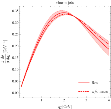
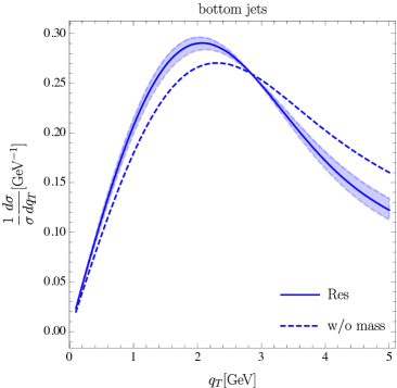
Figure 5: The normalized $q_{T}$-distribution for the unpolarized cross section of charm (left plot) and bottom (right plot) dijet production at the EIC. The solid curves are the results from using the resummation formula Eq. (2.8), while the dashed curves represent the resummation prediction using the evolution kernel without finite quark mass corrections. The red and blue bands indicate theoretical uncertainties from the variation of hard and jet scales as discussed in the text.

As given in the calculation of the jet function, we consider HF jets constructed using the anti-$k_{T}$ algorithm with radius $R=0.6$. The corresponding kinematic cuts for charm and bottom jets in the Breit frame are

$${\rm charm~{}jets:} ~{}~{}5\,{\rm GeV}<p_{T}<10\,{\rm GeV},\quad|y_{J}|<4.5\,,$$

$${\rm bottom~{}jets:} ~{}~{}10\,{\rm GeV}<p_{T}<15\,{\rm GeV},\quad|y_{J}|<4.5\,,$$ (83)

respectively. The charm and bottom quark masses are chosen as $m_{c}=1.5\,{\rm GeV}$ and $m_{b}=5\,{\rm GeV}$. The spin asymmetry from the gluon Sivers function is defined as

$$A_{UT}^{\sin(\phi_{q}-\phi_{s})}=2\frac{\int d\phi_{s}d\phi_{q}\sin(\phi_{q}-\phi_{s})\,d\sigma^{UT}(\bm{S}_{T})}{\int d\phi_{s}d\phi_{q}\,d\sigma^{UU}}\,.$$ (84)

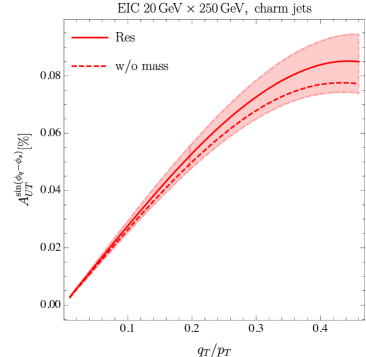
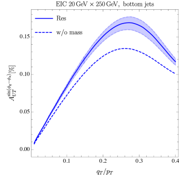
Figure 6: The Sivers spin asymmetry for charm (left plot) and bottom (right plot) dijet production at the EIC is plotted as a function of $q_{T}/p_{T}$. The solid curves are the results from using the resummation formula, while the dashed curves represent the resummation prediction using the evolution kernel without finite quark mass corrections. The red and blue bands indicate theoretical uncertainties from the variation of hard and jet scales.

In Fig. 5, we display the normalized unpolarized cross section, $1/\sigma\,d\sigma/dq_{T}$, as a function of the imbalance $q_{T}$. In Fig. 6, the Sivers spin asymmetry $A_{UT}^{\sin(\phi_{q}-\phi_{s})}$ is presented as a function of $q_{T}/p_{T}$ following Arratia:2020nxw , for both charm (left panel) and bottom (right panel) jets, respectively. For both plots, the solid curves are the results obtained using the resummation formula, while the dashed curves represent the resummation prediction using the evolution kernel without finite quark mass corrections. For both the unpolarized $q_{T}$ and $A_{UT}^{\sin(\phi_{q}-\phi_{s})}$ distributions, we find that the effects of the finite quark masses are modest for charm jets and quite sizable for bottom jets. This can be attributed to the sizes of the charm and bottom masses relative to their associated jet scales $p_{T}R$. As discussed in Secs. 2.5 and 2.6, we have that $J_{\mathcal{Q}}\rightarrow J_{q}$ and $S^{c}_{\mathcal{Q}}\rightarrow S^{c}_{q}$ as $m_{\mathcal{Q}}\rightarrow 0$, making them analytic functions of $m_{\mathcal{Q}}$ in the neighborhood of zero mass. Since Eqs. (2.8) and (2.8) carry their mass-dependence through the anomalous dimensions for the jet and collinear-soft functions, Eqs. (56) and (68), one sees that the massive versions of these functions are connected to the massless versions by the ratio $m_{\mathcal{Q}}/\left(p_{T}R\right)$–it is in fact this dimensionless parameter that controls the physical size of the mass corrections. With this in mind, one sees that Eq. (3) naturally positions bottom dijets further (in terms of the parameter $m_{\mathcal{Q}}/\left(p_{T}R\right)$) from light flavor jet-pairs than it does charm dijets. This relative positioning is then clearly displayed in Figs. 5 and 6.

In order to estimate the theoretical uncertainties, in both Figs. 5 and 6 we also show the uncertainties from scale variations, which are given by the red and blue bands. Here we vary the hard and jet scales by a factor of two around their default values as defined in (82), and the total uncertainty bands are obtained by the envelope of all the variations. Since the non-perturbative Sudakov factor in Eq. (79) is fitted at the canonical scale $\mu_{b_{*}}$, we do not include theory uncertainties from $\mu_{b_{*}}$ and $\mu_{cs}$ variations. We find that the scale uncertainty is compatible with the finite quark mass corrections in charm dijet process, while its impact on the bottom dijet process is smaller than the mass correction. Therefore in order to identify the finite quark mass effects in the charm dijet process it is essential to reduce the scale uncertainties. Our factorization and resummation formula provides a clear structure to improve the perturbative accuracy, which makes scale uncertainty further reduction possible. We leave the higher-order perturbative calculations in future work.

4 Conclusion

A major priority of the future EIC is to explore the gluon TMD PDFs. In this paper, we have investigated the use of back-to-back HF dijet production in transversely-polarized target DIS as a means of probing spin-dependent gluon TMD PDFs. We have calculated the expressions for the mass-dependent jet and collinear-soft functions at next-to-leading order. Using these expressions, as well as Soft-Collinear Effective Theory, we resum the large logarithms associated with these expressions at next-to-leading logarithmic accuracy. We then provide a factorization theorem for this process with QCD evolution in the kinematic region where heavy quark mass $m_{\mathcal{Q}}\lesssim p_{T}R\ll p_{T}$, with $p_{T}$ and $R$ being the transverse momentum and the radius of the jet, respectively. Furthermore, we generate a prediction for the Sivers asymmetry for charm and bottom dijets at the EIC, which can be used to probe the gluon Sivers function. We carefully study the effects of the HF masses by comparing our mass-dependent predicted asymmetry against the asymmetry in the massless limit. We find that, in the kinematic region we consider, the HF masses generate modest corrections to the predicted asymmetry for charm dijet production but sizable corrections for the bottom dijet process. Furthermore, we also consider the theoretical uncertainties from the scale variation. We find that the scale uncertainty can be compatible with the corrections from finite quark mass effects, especially for charm dijets production. In order to identify the mass effects and reduce the scale uncertainties one has to include higher-order corrections in the matching coefficients and the corresponding anomalous dimensions in Eqs. (2.8) and (2.8), and we leave the detailed perturbative calculations in future work.

References

- (1) A. Accardi et al., Electron Ion Collider: The Next QCD Frontier: Understanding the glue that binds us all, Eur. Phys. J. A 52 (2016) 268, [1212.1701].
- (2) D. Boer, P. J. Mulders, C. Pisano and J. Zhou, Asymmetries in Heavy Quark Pair and Dijet Production at an EIC, JHEP 08 (2016) 001, [1605.07934].
- (3) F. Yuan, Heavy Quarkonium Production in Single Transverse Polarized High Energy Scattering, Phys. Rev. D 78 (2008) 014024, [0801.4357].
- (4) A. Mukherjee and S. Rajesh, production in polarized and unpolarized ep collision and Sivers and asymmetries, Eur. Phys. J. C 77 (2017) 854, [1609.05596].
- (5) S. Rajesh, R. Kishore and A. Mukherjee, Sivers effect in Inelastic Photoproduction in Collision in Color Octet Model, Phys. Rev. D 98 (2018) 014007, [1802.10359].
- (6) A. Bacchetta, D. Boer, C. Pisano and P. Taels, Gluon TMDs and NRQCD matrix elements in production at an EIC, Eur. Phys. J. C 80 (2020) 72, [1809.02056].
- (7) D. Boer, U. D’Alesio, F. Murgia, C. Pisano and P. Taels, J/ meson production in SIDIS: matching high and low transverse momentum, JHEP 09 (2020) 040, [2004.06740].
- (8) U. D’Alesio, F. Murgia, C. Pisano and P. Taels, Azimuthal asymmetries in semi-inclusive production at an EIC, Phys. Rev. D 100 (2019) 094016, [1908.00446].
- (9) D. Boer et al., Gluons and the quark sea at high energies: Distributions, polarization, tomography, 1108.1713.
- (10) L. Zheng, E. Aschenauer, J. Lee, B.-W. Xiao and Z.-B. Yin, Accessing the gluon Sivers function at a future electron-ion collider, Phys. Rev. D 98 (2018) 034011, [1805.05290].
- (11) T. Sjostrand, S. Mrenna and P. Z. Skands, PYTHIA Physics and Manual, JHEP 05 (2006) 026, [hep-ph/0603175].
- (12) HERMES collaboration, A. Airapetian et al., Leading-Order Determination of the Gluon Polarization from high- Hadron Electroproduction, JHEP 08 (2010) 130, [1002.3921].
- (13) S. J. Brodsky, D. S. Hwang and I. Schmidt, Final state interactions and single spin asymmetries in semiinclusive deep inelastic scattering, Phys. Lett. B 530 (2002) 99–107, [hep-ph/0201296].
- (14) J. C. Collins, Leading twist single transverse-spin asymmetries: Drell-Yan and deep inelastic scattering, Phys. Lett. B 536 (2002) 43–48, [hep-ph/0204004].
- (15) D. Boer, P. Mulders and F. Pijlman, Universality of T odd effects in single spin and azimuthal asymmetries, Nucl. Phys. B 667 (2003) 201–241, [hep-ph/0303034].
- (16) M. Buffing, A. Mukherjee and P. Mulders, Generalized Universality of Definite Rank Gluon Transverse Momentum Dependent Correlators, Phys. Rev. D 88 (2013) 054027, [1306.5897].
- (17) D. Boer, C. Lorcé, C. Pisano and J. Zhou, The gluon Sivers distribution: status and future prospects, Adv. High Energy Phys. 2015 (2015) 371396, [1504.04332].
- (18) A. Arbuzov et al., On the physics potential to study the gluon content of proton and deuteron at NICA SPD, 2011.15005.
- (19) A. Banfi, M. Dasgupta and Y. Delenda, Azimuthal decorrelations between QCD jets at all orders, Phys. Lett. B 665 (2008) 86–91, [0804.3786].
- (20) S. D. Ellis and D. E. Soper, Successive combination jet algorithm for hadron collisions, Phys. Rev. D 48 (1993) 3160–3166, [hep-ph/9305266].
- (21) M. Dasgupta and G. P. Salam, Resummation of nonglobal QCD observables, Phys. Lett. B512 (2001) 323–330, [hep-ph/0104277].
- (22) D. Gutierrez-Reyes, I. Scimemi, W. J. Waalewijn and L. Zoppi, Transverse momentum dependent distributions with jets, Phys. Rev. Lett. 121 (2018) 162001, [1807.07573].
- (23) D. Gutierrez-Reyes, I. Scimemi, W. J. Waalewijn and L. Zoppi, Transverse momentum dependent distributions in and semi-inclusive deep-inelastic scattering using jets, JHEP 10 (2019) 031, [1904.04259].
- (24) M. G. A. Buffing, Z.-B. Kang, K. Lee and X. Liu, A transverse momentum dependent framework for back-to-back photon+jet production, 1812.07549.
- (25) X. Liu, F. Ringer, W. Vogelsang and F. Yuan, Lepton-jet Correlations in Deep Inelastic Scattering at the Electron-Ion Collider, Phys. Rev. Lett. 122 (2019) 192003, [1812.08077].
- (26) X. Liu, F. Ringer, W. Vogelsang and F. Yuan, Lepton-jet Correlation in Deep Inelastic Scattering, 2007.12866.
- (27) Y.-T. Chien, D. Y. Shao and B. Wu, Resummation of Boson-Jet Correlation at Hadron Colliders, JHEP 11 (2019) 025, [1905.01335].
- (28) Z.-B. Kang, K. Lee, D. Y. Shao and J. Terry, The Sivers Asymmetry in Hadronic Dijet Production, 2008.05470.
- (29) R. F. del Castillo, M. G. Echevarria, Y. Makris and I. Scimemi, TMD factorization for di-jet and heavy meson pair in DIS, 2008.07531.
- (30) J. Collins, Foundations of perturbative QCD, vol. 32. Cambridge University Press, 11, 2013.
- (31) M. A. Ebert, I. W. Stewart and Y. Zhao, Towards Quasi-Transverse Momentum Dependent PDFs Computable on the Lattice, JHEP 09 (2019) 037, [1901.03685].
- (32) B. Jager, M. Stratmann and W. Vogelsang, Single inclusive jet production in polarized collisions at , Phys. Rev. D 70 (2004) 034010, [hep-ph/0404057].
- (33) A. Mukherjee and W. Vogelsang, Jet production in (un)polarized pp collisions: dependence on jet algorithm, Phys. Rev. D 86 (2012) 094009, [1209.1785].
- (34) M. Dasgupta, F. A. Dreyer, G. P. Salam and G. Soyez, Inclusive jet spectrum for small-radius jets, JHEP 06 (2016) 057, [1602.01110].
- (35) X. Liu, S.-O. Moch and F. Ringer, Phenomenology of single-inclusive jet production with jet radius and threshold resummation, Phys. Rev. D 97 (2018) 056026, [1801.07284].
- (36) J.-Y. Chiu, A. Jain, D. Neill and I. Z. Rothstein, A Formalism for the Systematic Treatment of Rapidity Logarithms in Quantum Field Theory, JHEP 05 (2012) 084, [1202.0814].
- (37) M. G. Echevarria, T. Kasemets, P. J. Mulders and C. Pisano, QCD evolution of (un)polarized gluon TMDPDFs and the Higgs -distribution, JHEP 07 (2015) 158, [1502.05354].
- (38) P. Mulders and J. Rodrigues, Transverse momentum dependence in gluon distribution and fragmentation functions, Phys.Rev. D63 (2001) 094021, [hep-ph/0009343].
- (39) C. Bomhof and P. J. Mulders, Non-universality of transverse momentum dependent parton distribution functions, Nucl. Phys. B 795 (2008) 409–427, [0709.1390].
- (40) J. G. Korner, E. Mirkes and G. A. Schuler, QCD Jets at HERA. 1. Radiative Corrections to Electroweak Cross-sections and Jet Rates, Int. J. Mod. Phys. A4 (1989) 1781.
- (41) E. Mirkes and S. Willfahrt, Effects of jet azimuthal angular distributions on dijet production cross-sections in DIS, Phys. Lett. B 414 (1997) 205–209, [hep-ph/9708231].
- (42) W. Giele and E. Glover, Higher order corrections to jet cross-sections in annihilation, Phys. Rev. D 46 (1992) 1980–2010.
- (43) P. B. Arnold and M. H. Reno, The Complete Computation of High W and Z Production in 2nd Order QCD, Nucl. Phys. B319 (1989) 37–71.
- (44) S. Catani, The Singular behavior of QCD amplitudes at two loop order, Phys. Lett. B 427 (1998) 161–171, [hep-ph/9802439].
- (45) T. Becher and M. Neubert, Infrared singularities of scattering amplitudes in perturbative QCD, Phys. Rev. Lett. 102 (2009) 162001, [0901.0722].
- (46) J.-W. Qiu, W. Vogelsang and F. Yuan, Single Transverse-Spin Asymmetry in Hadronic Dijet Production, Phys. Rev. D 76 (2007) 074029, [0706.1196].
- (47) C. Bomhof and P. Mulders, Gluonic pole cross-sections and single spin asymmetries in hadron-hadron scattering, JHEP 02 (2007) 029, [hep-ph/0609206].
- (48) Z.-B. Kang and J.-W. Qiu, Single transverse-spin asymmetry for D-meson production in semi-inclusive deep inelastic scattering, Phys. Rev. D 78 (2008) 034005, [0806.1970].
- (49) U. D’Alesio, L. Maxia, F. Murgia, C. Pisano and S. Rajesh, Process dependence of the gluon Sivers function in within a TMD scheme in NRQCD, Phys. Rev. D 102 (2020) 094011, [2007.03353].
- (50) Z.-B. Kang, X. Liu, F. Ringer and H. Xing, The transverse momentum distribution of hadrons within jets, JHEP 11 (2017) 068, [1705.08443].
- (51) A. Hornig, D. Kang, Y. Makris and T. Mehen, Transverse Vetoes with Rapidity Cutoff in SCET, JHEP 12 (2017) 043, [1708.08467].
- (52) S. Fleming, A. H. Hoang, S. Mantry and I. W. Stewart, Jets from massive unstable particles: Top-mass determination, Phys. Rev. D 77 (2008) 074010, [hep-ph/0703207].
- (53) S. Fleming, A. H. Hoang, S. Mantry and I. W. Stewart, Top Jets in the Peak Region: Factorization Analysis with NLL Resummation, Phys. Rev. D 77 (2008) 114003, [0711.2079].
- (54) C. Lepenik and V. Mateu, NLO Massive Event-Shape Differential and Cumulative Distributions, JHEP 03 (2020) 024, [1912.08211].
- (55) A. Bris, V. Mateu and M. Preisser, Massive event-shape distributions at N2LL, JHEP 09 (2020) 132, [2006.06383].
- (56) A. H. Hoang, C. Lepenik and M. Stahlhofen, Two-Loop Massive Quark Jet Functions in SCET, JHEP 08 (2019) 112, [1904.12839].
- (57) L. Dai, C. Kim and A. K. Leibovich, Heavy Quark Jet Fragmentation, JHEP 09 (2018) 109, [1805.06014].
- (58) H. T. Li and I. Vitev, Inclusive heavy flavor jet production with semi-inclusive jet functions: from proton to heavy-ion collisions, JHEP 07 (2019) 148, [1811.07905].
- (59) C. Kim, Exclusive heavy quark dijet cross section, J. Korean Phys. Soc. 77 (2020) 469–476, [2008.02942].
- (60) M. Cacciari, G. P. Salam and G. Soyez, The anti- jet clustering algorithm, JHEP 04 (2008) 063, [0802.1189].
- (61) M. Balsiger, T. Becher and A. Ferroglia, Resummation of non-global logarithms in cross sections with massive particles, JHEP 09 (2020) 029, [2006.00014].
- (62) S. Catani and M. Grazzini, Higgs Boson Production at Hadron Colliders: Hard-Collinear Coefficients at the NNLO, Eur. Phys. J. C 72 (2012) 2013, [1106.4652].
- (63) T. Gehrmann, T. Luebbert and L. L. Yang, Calculation of the transverse parton distribution functions at next-to-next-to-leading order, JHEP 06 (2014) 155, [1403.6451].
- (64) T. Lübbert, J. Oredsson and M. Stahlhofen, Rapidity renormalized TMD soft and beam functions at two loops, JHEP 03 (2016) 168, [1602.01829].
- (65) M. G. Echevarria, I. Scimemi and A. Vladimirov, Unpolarized Transverse Momentum Dependent Parton Distribution and Fragmentation Functions at next-to-next-to-leading order, JHEP 09 (2016) 004, [1604.07869].
- (66) M.-X. Luo, T.-Z. Yang, H. X. Zhu and Y. J. Zhu, Transverse Parton Distribution and Fragmentation Functions at NNLO: the Gluon Case, JHEP 01 (2020) 040, [1909.13820].
- (67) M. A. Ebert, B. Mistlberger and G. Vita, Transverse momentum dependent PDFs at N3LO, 2006.05329.
- (68) P. Sun, J. Isaacson, C. P. Yuan and F. Yuan, Nonperturbative functions for SIDIS and Drell–Yan processes, Int. J. Mod. Phys. A 33 (2018) 1841006, [1406.3073].
- (69) J. C. Collins, D. E. Soper and G. F. Sterman, Transverse Momentum Distribution in Drell-Yan Pair and W and Z Boson Production, Nucl. Phys. B250 (1985) 199–224.
- (70) X.-D. Ji, Gluon correlations in the transversely polarized nucleon, Phys. Lett. B 289 (1992) 137–142.
- (71) H. Beppu, Y. Koike, K. Tanaka and S. Yoshida, Contribution of Twist-3 Multi-Gluon Correlation Functions to Single Spin Asymmetry in Semi-Inclusive Deep Inelastic Scattering, Phys. Rev. D 82 (2010) 054005, [1007.2034].
- (72) J.-w. Qiu and G. F. Sterman, Single transverse spin asymmetries, Phys. Rev. Lett. 67 (1991) 2264–2267.
- (73) J.-w. Qiu and G. F. Sterman, Single transverse spin asymmetries in direct photon production, Nucl. Phys. B 378 (1992) 52–78.
- (74) L.-Y. Dai, Z.-B. Kang, A. Prokudin and I. Vitev, Next-to-leading order transverse momentum-weighted Sivers asymmetry in semi-inclusive deep inelastic scattering: the role of the three-gluon correlator, Phys. Rev. D 92 (2015) 114024, [1409.5851].
- (75) I. Scimemi, A. Tarasov and A. Vladimirov, Collinear matching for Sivers function at next-to-leading order, JHEP 05 (2019) 125, [1901.04519].
- (76) COMPASS collaboration, C. Adolph et al., First measurement of the Sivers asymmetry for gluons using SIDIS data, Phys. Lett. B 772 (2017) 854–864, [1701.02453].
- (77) M. Burkardt, Sivers mechanism for gluons, Phys. Rev. D69 (2004) 091501, [hep-ph/0402014].
- (78) U. D’Alesio, F. Murgia and C. Pisano, Towards a first estimate of the gluon Sivers function from AN data in pp collisions at RHIC, JHEP 09 (2015) 119, [1506.03078].
- (79) E. Aschenauer, U. D’Alesio and F. Murgia, TMDs and SSAs in hadronic interactions, Eur. Phys. J. A 52 (2016) 156, [1512.05379].
- (80) U. D’Alesio, C. Flore, F. Murgia, C. Pisano and P. Taels, Unraveling the Gluon Sivers Function in Hadronic Collisions at RHIC, Phys. Rev. D 99 (2019) 036013, [1811.02970].
- (81) M. G. Echevarria, A. Idilbi, Z.-B. Kang and I. Vitev, QCD Evolution of the Sivers Asymmetry, Phys. Rev. D89 (2014) 074013, [1401.5078].
- (82) S. Dulat, T.-J. Hou, J. Gao, M. Guzzi, J. Huston, P. Nadolsky et al., New parton distribution functions from a global analysis of quantum chromodynamics, Phys. Rev. D 93 (2016) 033006, [1506.07443].
- (83) M. Arratia, Z.-B. Kang, A. Prokudin and F. Ringer, Jet-based measurements of Sivers and Collins asymmetries at the future electron-ion collider, Phys. Rev. D 102 (2020) 074015, [2007.07281].