Domain Adaptation with Incomplete Target Domains

Abstract

Domain adaptation, as a task of reducing the annotation cost in a target domain by exploiting the existing labeled data in an auxiliary source domain, has received a lot of attention in the research community. However, the standard domain adaptation has assumed perfectly observed data in both domains, while in real world applications the existence of missing data can be prevalent. In this paper, we tackle a more challenging domain adaptation scenario where one has an incomplete target domain with partially observed data. We propose an Incomplete Data Imputation based Adversarial Network (IDIAN) model to address this new domain adaptation challenge. In the proposed model, we design a data imputation module to fill the missing feature values based on the partial observations in the target domain, while aligning the two domains via deep adversarial adaption. We conduct experiments on both cross-domain benchmark tasks and a real world adaptation task with imperfect target domains. The experimental results demonstrate the effectiveness of the proposed method.

Introduction

Although deep learning models have achieved great success in many application domains (Krizhevsky, Sutskever, and Hinton 2012), their efficacy depends on the availability of large amounts of labeled training data. However, in practice it is often expensive or time-consuming to obtain labeled data. Domain adaptation tackles this key issue by exploiting a label-rich source domain to help learn a prediction model for a label-scarce target domain (Ben-David et al. 2007). The standard domain adaptation task assumes perfectly observed data in both the source and target domains, and centers the challenge of domain adaptation on bridging the cross-domain distribution gap. However, in real world applications the existence of missing data can be prevalent due to the difficulty of collecting complete data features. For example, in a service platform, a new user often chooses to fill minimal information during the registration process while skipping many optional entries. The incompleteness of such characteristic data can negatively impact the personalized recommendation or advertising strategies adopted by the service platforms. In such cases, the attempt of using active users’ data to help make predictions on new users’ preferences will not only form a domain adaptation problem but also entail an incomplete target domain with partially observed instances. Directly applying the standard domain adaptation methods in this scenario may fail to produce satisfactory results due to the ignorance of data incompleteness.

In this paper, we propose an adversarial domain adaptation model, named as Incomplete Data Imputation based Adversarial Network (IDIAN), to address the challenge of domain adaptation with incomplete target domains. The goal is to learn a good classifier in the target domain by effectively exploiting the fully observed and labeled data in the source domain. The model is designed to handle both homogeneous and heterogeneous cross-domain feature spaces in a semi-supervised setting. In this model, we represent each incomplete instance as a pair of an observed instance and a corresponding missing value indication mask, and use a data generator to fill the missing entries indicated by the mask based on the observed part. To ensure the suitability of the imputed missing data, we first use domain specific feature extractors to transform both the source domain data and the imputed target domain data into a unified feature space, and then deploy an inter-domain contrastive loss to push the cross-domain instance pairs that belong to the same class to have similar feature representations. To prevent spontaneous cross-domain feature affiliation and overfitting to the discriminative class labels, we introduce a domain specific decoder in each domain to regularize the feature extractors under autoencoder frameworks. Moreover, we introduce a domain discriminator to adversarially align the source and target domains in a further transformed common feature space, while the classifier can be trained in the same space. By simultaneously performing missing data imputation and bridging the cross-domain divergence gap, we expect the proposed model can provide an effective knowledge transfer from the source to the target domain and induce a good target domain classifier.

To test the proposed model, we conduct experiments on a number of cross-domain benchmark tasks by simulating the incomplete target domains. In addition, we also test our approach on a real-world ride-hailing service request prediction problem, which naturally has incomplete data in the target domain. The experimental results demonstrate the effectiveness of our proposed model by comparing with existing adversarial domain adaptation methods.

Related Work

Learning with Incomplete Data

Due to the difficulty of collecting entire feature set values in many application domains, learning with incomplete data has been a significant challenge in supervised classification model training. The work of (Little and Rubin 2014) provides a systematic study for data analysis problems with different data missing mechanisms. The naive approach of dealing with missing data is using only the partial observations; that is, one deletes all entries (or rows) with missing values before deploying the data for model training. Alternatively, the most common strategy is to attempt to impute the missing values.

Early imputation approaches use some general probabilistic methods to estimate or infer the values of the missing entries. For example, the work in (Dempster, Laird, and Rubin 1977) uses the Expectation-Maximum algorithm (EM) to handle latent variables and the work in (Honaker et al. 2011) uses multivariate normal likelihoods for learning with missing values. These methods however require prior knowledge of the underlying model structure. Alternatively, the sequential regression in (Raghunathan 2016) provides a variable-by-variable input technique for missing value imputation. The multivariate imputation by chained equations (MICE) in (Buuren and Groothuis-Oudshoorn 2010) provides a multi-category representation of the chain equation. Then linear regression was used for the value estimation of ordinal variables and multivariate logistic regression was used for categorical variables. These approaches however can suffer from computational problems when there are too many missing variable values.

Recently, deep learning approaches have been adopted for handling missing values. In particular, the generative adversarial networks (GAN) have been adapted as a common approach for missing value imputation. For example, the authors of (Yoon, Jordon, and Schaar 2018) proposed generative adversarial imputation nets (GAIN), which imputes the missing data with a generation network. The AmbientGAN method developed in (Bora, Price, and Dimakis 2018) trains a generative model directly from noisy or incomplete samples. The MisGAN in (Li, Jiang, and Marlin 2019) learns a mask distribution to model the missingness and uses the masks to generate complete data by filling the missing values with a constant value. Nevertheless, these methods focus on (semi-)supervised learning. In another work (Kirchmeyer et al. 2019) that has recently been brought into our attention, the authors propose to address homogeneous unsupervised domain adaptation with data imputation by learning a data generator after feature mapping in the source domain. In contrast, our proposed model addresses supervised domain adaptation with incomplete target domains, accommodating both homogeneous and heterogeneous cross-domain input feature spaces.

Generative Adversarial Networks

Generative adversarial networks (GANs) (Goodfellow et al. 2014) generate samples that are indistinguishable from the real data by playing a minimax game between a generator and a discriminator. DCGAN greatly improves the stability of GAN training by improving the architecture of the initial GAN and modifying the network parameters (Mandal, Puhan, and Verma 2018). CGAN generates better quality images by using additional label information and is able to control the appearance of the generated images to some extent (Mirza and Osindero 2014). Wasserstein GAN uses the Wasserstein distance to increase the standard GAN’s training stability (Arjovsky, Chintala, and Bottou 2017). As already reviewed above, the GAN based models have also been developed to address learning with incomplete data.

Domain Adaptation

Domain adaptation aims to exploit label-rich source domains to solve the problem of insufficient training data in a target domain (Ben-David et al. 2007). The research effort on domain adaptation has been mostly focused on bridging the cross-domain divergence. For example, Ghifary et al. proposed to use autoencoders in the target domain to obtain domain-invariant features (Ghifary et al. 2016). The work in (Sener et al. 2016) proposes using clustering techniques and pseudo-labels to obtain discriminative features. Taigman et al. proposed cross-domain image translation methods (Taigman, Polyak, and Wolf 2016).

The authors of (Ben-David et al. 2007) developed theoretical results on domain adaptation that suggest the expected prediction risk of a source classifier in the target domain is bounded by the divergence of the distributions. Motivated by the theoretical work, matching distributions of extracted features has been considered to be effective in realizing an accurate adaptation (Bousmalis et al. 2016; Purushotham et al. 2019; Li et al. 2018; Sun, Feng, and Saenko 2016). The representative method of distribution matching learns a domain adversarial neural network (DANN) by extracting features that deceive a domain discrimination classifier (Ganin et al. 2016). It extends the idea of generative adversarial networks into the domain adaptation setting by using the feature extraction network as a generator and using the domain classifier as a discriminator. The features that can maximumly confuse the discriminator are expected to effectively match the feature distributions across the source and target domains. The conditional domain adversarial network model (CDAN) further extends DANN by aligning the joint distribution of feature and category across domains (Long et al. 2018). In addition, some other methods have utilized the maximum mean discrepancy (MMD) criterion to measure the distribution divergence in high-dimensional space between different domains (Long et al. 2016, 2015), They train the model to simultaneously minimize both the MMD based cross-domain divergence and the prediction loss on the labeled training data. Nevertheless, all these domain adaptation methods assume fully observed data in both the source and target domains. In this paper, we address a novel domain adaptation setting where the target domain contains incomplete data.

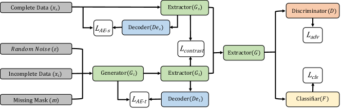
Figure 1: The overall structure of the proposed incomplete data imputation based adversarial network (IDIAN). It has the following components: (1) The incomplete data generator $G_{i}$ in the target domain. (2) The domain specific autoencoders in both domains, each of which is formed by a feature extractor and a decoder (($G_{s},De_{s}$) or ($G_{t},De_{t}$)). (3) The adversarial domain adapter, which is formed by a common feature extractor $G$, a domain discriminator $D$, and a classifier $F$.

Method

We consider the following domain adaptation setting. We have a source domain ${\it S}$ and a target domain ${\it T}$. The source domain has a large number ($n_{s}$) of labeled instances, $\mathcal{D}_{S}={\left\{(x_{i}^{s},y_{i}^{s})\right\}}_{i=1}^{n_{s}}$, where $x_{i}^{s}\in\mathcal{R}^{d_{s}}$ denotes the $i$-th instance and $y_{i}^{s}$ is a $\{0,1\}$-valued label indicator vector. In the target domain, we assume there are a very small number of labeled instances and all the other instances are unlabeled: $\mathcal{D}_{T}={\left\{(x_{i}^{t},m_{i}^{t},\cdot)\right\}}_{i=1}^{n_{t}}$, where $x_{i}^{t}\in\mathcal{R}^{d_{t}}$ denotes the $i$-th target instance, which is only partially observed and its entry observation status is encoded by a binary-valued mask vector $m_{i}^{t}\in\{0,1\}^{d_{t}}$. Without loss of generality, we assume the first $n_{l}$ instances are labeled, such that $\mathcal{D}_{T_{l}}={\left\{(x_{i}^{t},m_{i}^{t},y_{i}^{t})\right\}}_{i=1}^{n_{l}}$ and $\mathcal{D}_{T_{l}}\subseteq\mathcal{D}_{T}$. We further assume the class label spaces in the two domains are the same, while their input feature spaces can be either same ($\mathcal{R}^{d_{s}}=\mathcal{R}^{d_{t}}$) or different ($\mathcal{R}^{d_{s}}\not=\mathcal{R}^{d_{t}}$).

In this section, we present an incomplete data imputation based adversarial learning network (IDIAN) to address the challenging domain adaptation problem above. The proposed IDIAN model is illustrated in Figure 1. It has the following components: (1) The incomplete data generator $G_{i}$, which imputes the missing values in the target domain. (2) The domain specific autoencoders in both domains, each of which is formed by a feature extractor and a decoder (($G_{s},De_{s}$) or ($G_{t},De_{t}$)). They map the input data from both domains into a unified feature space by ensuring both information preservation via a reconstruction autoencoder loss ($L_{AE_{s}}$ or $L_{AE_{t}}$) and discriminative cross-domain alignment via an inter-domain contrastive loss ($L_{cont}$). (3) The adversarial domain adapter, which is formed by a common feature extractor $G$, a domain discriminator $D$, and a classifier $F$ after the cross-domain feature space unification. It performs adversarial cross-domain feature alignment to bridge the cross-domain divergence and induces a good classifier $F$. These components coordinate with each other under the proposed framework to facilitate the overall effective knowledge transfer and classifier training. Below we present these components and the overall learning objective in detail.

Incomplete Data Imputation

The existence of missing data in the target domain presents a significant challenge for domain adaptation. Simply ignoring the missing data or imputing the missing entries with non-informative zeros will unavoidably lead to information loss and degrade the adaptation performance. Meanwhile, one fundamental assumption of domain adaptation is that the source and target domains share the same prediction problem but present different data distributions or representation forms in the input feature space. This suggests that the suitable data imputation in the target domain should coherently support the common prediction model induction and the mitigation of the cross-domain divergence. In light of this understanding, we propose to simultaneously perform data imputation in the target domain, match the cross-domain data distributions and learn the classifier in an unified feature space under the end-to-end IDIAN learning framework. In particular, as shown in Figure 1, we introduce a generation network $G_{i}$ to perform data imputation within the IDIAN.

Typically different features (attributes) in the input space are not independent from each other but rather present correlations. Hence we propose to generate the missing values of each instance based on its observed entries. Specifically, our generator $G_{i}$ takes a triplet ($x^{t},m^{t},\varepsilon$) as input, where $x^{t}$ denotes the given partially observed instance in the target domain, $m^{t}$ is the corresponding mask vector with value 1 indicating an observed entry and value 0 indicating a missing entry, and $\varepsilon$ is a noise vector randomly sampled from a standard normal distribution. Then $G_{i}$ generates the imputed instance as follows:

$$G_{i}\left(x^{t},m^{t},\varepsilon\right)=x^{t}\odot m^{t}+\hat{G}_{i}\left(x^{t}\odot m^{t}+\varepsilon\odot\bar{m}^{t}\right)\odot\bar{m}^{t}$$ (1)

where $\bar{m}^{t}=1-m^{t}$ and “$\odot$” denotes the Hadamard product operation. Here the imputation network $\hat{G}$ fills the missing values of $x^{t}$, and the overall computation in Eq.(1) ensures the original observed features will not be modified.

Feature Space Unification with Discriminatively Aligned Autoencoders

The proposed IDIAN model allows heterogeneous cross-domain input feature spaces. Hence we introduce two domain specific feature extractors, $G_{s}$ and $G_{t}$, in the source and target domains respectively to transform the input features into a unified feature space. Moreover, to prevent information loss during the feature transformation we introduce two domain specific decoders, $De_{s}$ and $De_{t}$, to form autoencoders together with $G_{s}$ and $G_{t}$ in the source and target domains respectively. The principle of autoencoder learning lies in minimizing the reconstruction loss between the original input instances and their corresponding reconstructed versions which are obtained by feeding each instance through the feature extractor (encoder) and decoder. A small reconstruction error ensures the feature extractor to preserve essential information from the inputs. In the proposed model, we use the following reconstruction loss in the two domains:

$$L_{AE} =L_{AE_{s}}+L_{AE_{t}}$$ (2)

$$=\frac{1}{n_{s}}\sum\nolimits_{i=1}^{n_{s}}\left\|De_{s}\left(G_{s}\left(x_{i}^{s}\right)\right)-x_{i}^{s}\right\|^{2}+$$

$$\quad\frac{1}{n_{t}}\sum\nolimits_{i=1}^{n_{t}}\left\|De_{t}\left(G_{t}\left(\hat{x}_{i}^{t}\right)\right)-\hat{x}_{i}^{t}\right\|^{2}$$

where $\hat{x}_{i}^{t}$ denotes the imputed $i$-th instance in the target domain, such that $\hat{x}_{i}^{t}=G_{i}\left(x_{i}^{t},m_{i}^{t},\varepsilon\right)$.

Inter-Domain Contrastive Loss

As domain adaptation assumes a shared prediction problem in the unified feature representation space, we further propose to discriminatively align the extracted features of the instances from the two domains based on their corresponding labels, in order to ensure a unified feature space after the feature extraction. Specifically, we design the following inter-domain contrastive loss to promote the discriminative alignment of the instances across domains:

$$L_{cont}=\mathbb{E}_{(x_{i},x_{j})\sim\mathcal{D}_{S}\cup\mathcal{D}_{T_{l}}}L_{dis}\!\left(f_{i},f_{j},\delta\left(y_{i},y_{j}\right)\right)$$ (3)

where $\delta(y_{i},y_{j})$ is an identity indication function, which has value 1 when $y_{i}=y_{j}$ and has value 0 when $y_{i}\not=y_{j}$; $f_{i}$ and $f_{j}$ denote the extracted feature vectors for instances $x_{i}$ and $x_{j}$ respectively, such that

$$f_{i}=\left\{\begin{array}[]{ll}G_{s}(x_{i})&\mbox{if}\;x_{i}\in\mathcal{D}_{S},\\ G_{t}(G_{i}(x_{i},m_{i},\varepsilon))&\mbox{if}\;x_{i}\in\mathcal{D}_{T_{l}}.\\ \end{array}\right.$$ (6)

The contrastive distance function $L_{dis}$ is defined as:

$$L_{dis}=\left\{\begin{array}[]{ll}\left\|f_{i}-f_{j}\right\|^{2}&\mbox{if}\;\delta\left(y_{i},y_{j}\right)=1,\\ \max\left(0,\,\rho-\left\|f_{i}-f_{j}\right\|^{2}\right)&\mbox{if}\;\delta\left(y_{i},y_{j}\right)=0.\end{array}\right.$$ (7)

Here $\rho$ is a pre-defined margin value, which is used to control the distance margin between instances from different classes. This contrastive loss aims to reduce the intra-class distance and increase the inter-class distance over data from both the source and target domains in the unified feature space.

Adversarial Feature Alignment

The discriminatively aligned autoencoders above aim to induce a unified feature space. However, there might still be distribution divergence across domains. We therefore deploy an adversarial domain adaptation module to align the cross-domain feature distributions, while training a common classifier. As shown in Figure 1, the adversarial adaptation module consists of a feature extractor $G$, a domain discriminator $D$, and a classifier $F$. $D$ is a binary probabilistic classifier that assigns label 1 to the source domain and label 0 to the target domain. Following the principle of the adversarial training of neural networks, the module plays a minimax game between the feature extractor $G$ and the domain discriminator $D$ through the following adversarial loss:

$$L_{adv}= -\frac{1}{n_{s}}\sum\nolimits_{i=1}^{n_{s}}\log D\left(G(f_{i}^{s})\right)$$

$$-\frac{1}{n_{t}}\sum\nolimits_{j=1}^{n_{t}}\log\left(1-D\left(G(f_{i}^{t})\right)\right)$$ (8)

where $f_{i}^{s}=G_{s}(x_{i}^{s})$ and $f_{i}^{t}=G_{t}(G_{i}(x_{i}^{t},m_{i}^{t},\varepsilon))$. The domain discriminator $D$ will be trained to maximumly distinguish the two domains by minimizing this loss, while $G$ aims to produce suitable features to confuse $D$ by maximizing this adversarial loss and hence diminishing the cross-domain distribution gap. Meanwhile, we also train the classifier $F$ in the extracted feature space by minimizing the following cross-entropy classification loss on all the labeled instances:

$$L_{cls}= -\frac{1}{n_{l}}\sum\nolimits_{j=1}^{n_{l}}y_{j}^{t\top}\log F\left(G(f_{i}^{t})\right)$$

$$-\alpha\frac{1}{n_{s}}\sum\nolimits_{i=1}^{n_{s}}y_{i}^{s\top}\log F\left(G(f_{i}^{s})\right)$$ (9)

where $\alpha$ is a trade-off hyperparameter.

  Input: Training data $\mathcal{D}_{S}$ and $\mathcal{D}_{T}$; trade-off parameters $\alpha$, $\beta$, $\gamma$, and $\lambda$; constant margin $\rho$; epoch# $N_{e}$, batch size $n_{b}$

  Initialization: Randomly initialize the model parameters

  for  $k=1$ to $N_{e}$ do

     Randomly reshuffle $\mathcal{D}_{S}$ into a set of mini-batches $S_{B}=\{B_{1},B_{2},\cdots,B_{J}\}$ with batch size $n_{b}$

     for $j=1$ to $J$ do

        Randomly sample a batch $B_{l}^{t}$ from $\mathcal{D}_{T_{l}}$ with size $n_{b}$. Randomly sample a batch $B^{t}$ from $\mathcal{D}_{T}\setminus\mathcal{D}_{T_{l}}$ with size $n_{b}$. Set $B_{j}=B_{j}\cup B_{l}^{t}\cup B^{t}$

     end for

     for $B\in S_{B}$  do

        1. Generate imputed data for the incomplete target instances in $B$ using $G_{i}$ with Eq.(1)

        2. Compute the reconstruction loss $L_{AE}$ on imputed batch $B$ with Eq.(2)

        3. Compute the contrastive loss $L_{cont}$ on imputed batch $B$ with Eq.(3)

        4. Compute the adversarial loss $L_{adv}$ and the classification loss $L_{cls}$ with Eq.(8) and Eq.(9) respectively on imputed batch $B$

        5. Conduct gradient descent over parameters of each component network :

$$\Theta_{G_{i}},\Theta_{G_{s}},\Theta_{G_{t}}\overset{-}{\leftarrow}\; \eta\;\triangledown_{\Theta_{G_{i}},\Theta_{G_{s}},\Theta_{G_{t}}}\!L(\Theta)$$

$$\Theta_{De_{s}},\Theta_{De_{t}}\overset{-}{\leftarrow}\; \eta\;\triangledown_{\Theta_{De_{s}},\Theta_{De_{t}}}\!L_{AE}$$

$$\Theta_{G}\overset{-}{\leftarrow}\; \eta\;\triangledown_{\Theta_{G}}\!\left(L_{cls}\!+\!\gamma L_{cont}\!-\!\lambda L_{adv}\right)$$

$$\Theta_{D}\overset{+}{\leftarrow}\; \eta\;\triangledown_{\Theta_{D}}\left(\lambda L_{adv}\right)$$

$$\Theta_{F}\overset{-}{\leftarrow}\; \eta\;\triangledown_{\Theta_{F}}\left(L_{cls}\right)$$

     end for

  end for

Algorithm 1 Training algorithm for IDIAN

Overall Learning Problem

Finally, by integrating the autoencoders’ reconstruction loss, the contrastive loss, the adversarial loss, and the classification loss together, we have the following adversarial learning problem for the proposed IDIAN model:

$$\min_{G_{i}\!,G_{s}\!,G_{t}\!,G\!,F\!,De_{s}\!,De_{t}}\max_{D}\quad L(\Theta)$$ (10)

$$\mbox{where}\quad L(\Theta)=L_{cls}+\beta L_{AE}+\gamma L_{cont}-\lambda L_{adv}$$

where $\lambda$, $\beta$, $\gamma$ are trade-off parameters between different loss terms; $\Theta$ denotes the parameters for all the component networks (the whole model). The model is trained in an end-to-end fashion with stochastic gradient descent. The overall algorithm is illustrated in Algorithm 1.

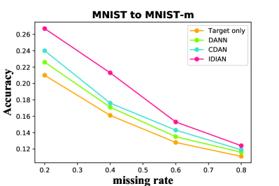
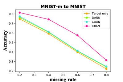
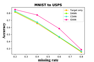
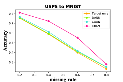
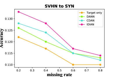
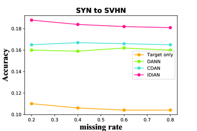
Figure 2: Test accuracy comparison of different domain adaptation methods with different data missing rates in the target domain. 10 instances per class in each target domain are used as the labeled data.

Table 1: Architecture details of IDIAN. ‘fc(x,y)’ denotes a fully connected layer with input size x and output size y. ‘relu’, ‘sigmoid’ and ‘softmax’ denote the activation functions. $d_{s}$ and $d_{t}$ denote the input feature dimension in the source and target domains respectively; $n_{c}$ denotes the number of classes.

	Architecture		Architecture
$G_{i}$	fc1($d_{t}$,512)-relu fc2(512,512)-relu fc3(512,512)-relu fc4(512,$d_{t}$)-sigmoid	$De_{s}$	fc1(1024,2048)-relu fc2(2048,$d_{s}$)
$G_{s}$	fc1($d_{s}$,2048)-relu fc2(2048,1024)	$De_{t}$	fc1(1024,2048)-relu fc2(2048,$d_{t}$)
$G_{t}$	fc1($d_{t}$,2048)-relu fc2(2048,1024)	$D$	fc1(256,512)-relu fc2(512,1)-sigmoid
$G$	fc1(1024,512)-relu fc2(512,256)	$F$	fc1(256,$n_{c}$)-softmax

Table 2: Comparison results over domain adaptation methods on the six constructed digit recognition domain adaptation tasks under the setting of 40% data missing rate and 10 labeled instances per class in the target domain.

Methods	MNIST$\to$ MNIST-M	MNIST-M$\to$ MNIST	MNIST$\to$ USPS	USPS$\to$ MNIST	SVHN$\to$ SYN	SYN$\to$ SVHN
Target only	0.161$\pm$0.003	0.592$\pm$0.007	0.656$\pm$0.005	0.589$\pm$0.005	0.117$\pm$0.002	0.106$\pm$0.002
DANN	0.171$\pm$0.006	0.607$\pm$0.006	0.669$\pm$0.004	0.594$\pm$0.007	0.120$\pm$0.003	0.159$\pm$0.006
CDAN	0.176$\pm$0.006	0.612$\pm$0.006	0.673$\pm$0.003	0.613$\pm$0.005	0.124$\pm$0.003	0.167$\pm$0.003
IDIAN	0.213$\pm$0.004	0.743$\pm$0.006	0.775$\pm$0.005	0.723$\pm$0.006	0.128$\pm$0.005	0.184$\pm$0.005

Table 3: Comparison results over domain adaptation methods on the six constructed digit recognition domain adaptation tasks under the setting of 40% data missing rate and 20 labeled instances per class in the target domain.

Methods	MNIST$\to$ MNIST-M	MNIST-M$\to$ MNIST	MNIST$\to$ USPS	USPS$\to$ MNIST	SVHN$\to$ SYN	SYN$\to$ SVHN
target only	0.172$\pm$0.003	0.691$\pm$0.004	0.750$\pm$0.003	0.689$\pm$0.004	0.130$\pm$0.004	0.113$\pm$0.002
DANN	0.177$\pm$0.009	0.710$\pm$0.007	0.753$\pm$0.017	0.706$\pm$0.003	0.135$\pm$0.008	0.192$\pm$0.018
CDAN	0.183$\pm$0.004	0.714$\pm$0.003	0.756$\pm$0.008	0.709$\pm$0.008	0.137$\pm$0.004	0.191$\pm$0.004
IDIAN	0.223$\pm$0.002	0.777$\pm$0.004	0.820$\pm$0.010	0.780$\pm$0.006	0.143$\pm$0.004	0.195$\pm$0.023

Table 4: Comparison results over domain adaptation methods on the real world ride-hailing dataset.

Methods	AUC	ACC	Recall	Precision	F1 score
Target only	0.564$\pm$0.006	0.564$\pm$0.006	0.568$\pm$0.006	0.563$\pm$0.006	0.566$\pm$0.009
DANN	0.580$\pm$0.002	0.580$\pm$0.002	0.588$\pm$0.005	0.578$\pm$0.006	0.584$\pm$0.008
CDAN	0.585$\pm$0.004	0.585$\pm$0.004	0.565$\pm$0.009	0.582$\pm$0.008	0.583$\pm$0.007
IDIAN	0.595$\pm$0.004	0.595$\pm$0.004	0.611$\pm$0.009	0.597$\pm$0.007	0.604$\pm$0.009

Table 5: The ablation study results on the task MNIST-M$\rightarrow$MNIST.

Methods	20% missing	40% missing	60% missing	80% missing
IDIAN w/o imputation	0.794$\pm$0.006	0.664$\pm$0.005	0.498$\pm$0.007	0.265$\pm$0.006
IDIAN w/o $L_{AE}$	0.790$\pm$0.006	0.640$\pm$0.008	0.453$\pm$0.005	0.264$\pm$0.003
IDIAN w/o $L_{contrast}$	0.802$\pm$0.005	0.731$\pm$0.006	0.561$\pm$0.007	0.296$\pm$0.007
IDIAN	0.814$\pm$0.005	0.743$\pm$0.006	0.575$\pm$0.006	0.312$\pm$0.005

Experiment

We conducted experiments on both benchmark digit recognition datasets for domain adaptation with simulated incomplete target domains and a real world domain adaptation problem with natural incomplete target domains for ride-hailing service request prediction. In this section, we present our experimental setting and results.

Experimental Settings

Digit Recognition Image Datasets

We used a set of commonly used domain adaptation tasks constructed on five types of digit recognition datasets. The five digital datasets are MNIST (LeCun et al. 1998), MNIST-M, Street View House Numbers (SVHN) (Netzer et al. 2011), Synthetic Numbers (SYN) (Moiseev et al. 2013) and USPS (Hull 1994). We contructed six common domain adaptation tasks by using these datasets as three pairs of domains: (1) MNIST $\leftrightarrow$ MNIST-M. MNIST-M is obtained from MNIST by blending digits from the original set over patches randomly extracted from color photos from BSDS500. We can have two domain adapation tasks by using each one as the source domain and the other one as the target domain. (2) SYN $\leftrightarrow$ SVHN. Synthetic numbers (SYN) consists of 500,000 synthesized images generated from Windows fonts. We put this synthesized digit image set together with real Street-View House Number dataset (SVHN) as adaptation domain pairs. Again, two domain adaptation tasks can be obtained by using one domain as the source domain and the other domain as the target domain, and then reversing the order. (3) MNIST $\leftrightarrow$ USPS. In the same manner as above, we also constructed two domain adaptation tasks between the USPS handwritten digit images and the MNIST set. We used an unsupervised Autoencoder model to extract features from raw images on each dataset, which we later used as the input data in our domain adaptation experiments. The encoder of the model consists of three convolutional layers, while the decoder is composed of three transpose convolutional layers. We resize each image to 32 x 32 x 3 as the input of the autoencoder, and the encoder maps each image into a 1024-dim feature vector.

As these standard domain adaptation tasks have fully observed data in both domains, we simultate the incomplete target domain by randomly setting part of the instance feature values as zeros in the target domain, indicating the missing status of the corresponding entries. We can create incomplete target domains with any feature missing rate between 0 and 1. Moreover, to further enhance the difference of the cross-domain features, we also randomly shifted the order of the feature channels in the target domains.

Ride-Hailing Service Request Adaptation Dataset

We collected a real world adaptation dataset with incomplete target domains from a ride-hailing service platform. The advertising needs on the ride-hailing service platform often requires the prediction of the service usage of new users given the historical service usage data of many active users. We treat this problem as a cross-domain binary classification problem over users, where the active users’ data form the source domain and the new users’ data form the target domain. As a new user’s information typically contains many missing entries, the target domain in this problem is naturally incomplete. We obtained a source domain with 400k instances of active users and a target domain with 400k instances of new users. Moreover, as the active users and the new users are collected in different time and manner, there is no record of the feature space correspondence between them though they do share many attributes. In the dataset, the feature dimension in the source domain is 2433 and in the target domain is 1302. Moreover, the feature missing rate in the target domain is very high, close to 89%.

Model Architecture

For the proposed IDIAN model, we used the multi-layer perceptrons for its components. Specifically, we used a four layer network for $G_{i}$. The feature extractors $\{G_{s},G_{t},G\}$, the decoders $\{De_{s},De_{t}\}$, and the discriminator $D$ are each composed of two fully connected layers respectively. The classifier $F$ is composed of one fully connected layer. The specific details are provided in Table 1.

Comparison Methods

This is the very first work that addresses the problem of domain adaptation with incomplete target domains. Moreover, our problem setting is very challenging such that the input feature spaces of the two domains can be different, Hence we compared our proposed IDIAN model with the following baseline and two adapted state-of-the-art adversarial domain adaptation methods: (1) Target only. This is a baseline method without domain adaptation, which trains a classification network with only the labeled data in the target domain. For fair comparison, we used the same architectures of feature extractor ($G_{t}$ and $G$) and classifier ($F$) as our proposed model. (2) DANN. This is an adversarial domain adaptation neural network developed in (Ganin et al. 2016). For fair comparison and also adapting DANN to handle different cross-domain feature spaces, we build DANN under the same framework as our proposed model by dropping $G_{i}$, $De_{s}$ and $De_{t}$, while only using the adversarial loss and classification loss as the optimization objective. (3) CDAN. This is a conditional adversarial domain adaptation network developed in (Long et al. 2018). It takes the instance’s class information as a joint input to the adversarial domain discriminator, aiming to address the multimodal structure of the feature alignment. Here, we build CDAN by adjusting the DANN above and providing the classifier’s label prediction results as input to the conditional adversarial domain discriminator.

Experiments on Image Datasets

For each of the six domain adaptation tasks constructed on the digital image datasets, we simulated the incomplete target domain in different situations by dropping out 20%/40%/60%/80% of the feature values respectively. We also conducted experiments by randomly selecting 10 or 20 labeled instances from each category as the labeled instances in the target domain and using the rest target data as unlabeled data.

In this set of experiments, we used a learning rate $\eta=0.01$ and set the batch size to 128. The trade off parameters of IDIAN (${\alpha,\beta,\gamma,\lambda}$) are set as (1,10,10,10). We set the epoch number $N_{e}$ as 20. We repeated each experiment five times, and recorded the mean accuracy and standard deviation values of the results on the test data of the target domain.

Results

Table 2 and Table 3 report the comparison results on the six domain adaptation tasks with a 40% feature missing rate in the target domain by using 10 and 20 instances from each class in the target domain as labeled instances respectively. We can see that in both tables, the Target only baseline produces the worst results across all domain adaptation tasks. With domain adaptation, both DANN and CDAN outperform Target only with notable margins, while CDAN produces even slightly better results than DANN. Nevertheless, the proposed IDIAN produced the best results among all the comparison methods across all the six tasks.

We also experimented with different feature missing rates in the target domain. The six sub-figures in Figure 2 present the comparison results on the six domain adaptation tasks respectively across multiple feature missing rates (20%, 40%, 60%, 80%) in the target domain. Again, we can see our proposed IDIAN consistently outperforms all the other methods across all scenarios. These results demonstrated the efficacy of our proposed model.

Experiments on Ride-Hailing Dataset

On this real world incomplete domain adaptation task, we used 50% of the target domain data for training and the remaining 50% for testing. On the training data, we randomly chose 1000 instances in the target domain as labeled instances ($n_{l}=1000$). All the data in the source domain are used as training data. We used a learning rate $\eta=0.01$ and set the batch size as 500. We set the trade off parameters (${\alpha,\beta,\gamma,\lambda}$) as (5,20,20,20) respectively, and set the epoch number as 50. We repeated the experiment five times, and recorded the mean and standard deviation values of the test results.

Results

For this binary classification task, we evaluated the test performance using five different measures: AUC, ACC (accuracy), recall, precision and F1 score. The comparison results are reported in Table 4. We can see that, similar to previous results, all the domain adaptation methods outperform the Target only baseline. This verified the efficacy of the domain adapation mechanism even in this much challenging real world learning scenario. Moreover, the proposed IDIAN further outperforms both DANN and CDAN in terms of all the five different measures. In terms of F1 score, IDIAN outperforms the baseline by 3.8%. The results validated the efficacy of our proposed model.

Ablation Study

To further analyze the proposed IDIAN model, we conducted an ablation study on the adaptation task from MNIST-M$\rightarrow$ MNIST with 10 labeled instances from each target class. Specifically, we compared the full IDIAN model with the following three variants: (1) IDIAN w/o imputation. This variant drops the incomplete data imputation component in IDIAN. (2) IDIAN w/o $L_{AE}$. This variant drops the decoders and the Autoencoder loss $L_{AE}$ in IDIAN. (3) IDIAN w/o $L_{cont}$. This variant drops the inter-domain contrastive loss $L_{cont}$ in IDIAN. The comparison results are reported in Table 5 We can see that the performance of all the variants are much inferior to the full IDIAN model. The results are consistent across settings with different target feature missing rates, which validated the essential contribution of the data imputation, autoencoder, and inter-domain contrastive loss for the proposed IDIAN model.

Conclusion

In this paper, we addressed a novel domain adaptation scenario where the data in the target domain are incomplete. We proposed an Incomplete Data Imputation based Adversarial Network (IDIAN) model to address this new domain adaptation challenge. The model is designed to handle both homogeneous and heterogeneous cross-domain feature spaces. It integrates data dependent feature imputation, autoencoder-based cross-domain feature space unification, and adversarial domain adaptation coherently into an end-to-end deep learning model. We conducted experiments on both cross-domain benchmark tasks with simulated incomplete target domains and a real-world adaptation problem on ride-hailing service request prediction with natural incomplete target domains. The experimental results demonstrated the effectiveness of the proposed model.

References

- Arjovsky, Chintala, and Bottou (2017) Arjovsky, M.; Chintala, S.; and Bottou, L. 2017. Wasserstein Generative Adversarial Networks. In International Conference on Machine Learning.
- Ben-David et al. (2007) Ben-David, S.; Blitzer, J.; Crammer, K.; and Pereira, F. 2007. Analysis of representations for domain adaptation. In Advances in neural information processing systems.
- Bora, Price, and Dimakis (2018) Bora, A.; Price, E.; and Dimakis, A. G. 2018. AmbientGAN: Generative models from lossy measurements. In International Conference on Learning Representations.
- Bousmalis et al. (2016) Bousmalis, K.; Trigeorgis, G.; Silberman, N.; Krishnan, D.; and Erhan, D. 2016. Domain separation networks. In Advances in neural information processing systems.
- Buuren and Groothuis-Oudshoorn (2010) Buuren, S. v.; and Groothuis-Oudshoorn, K. 2010. mice: Multivariate imputation by chained equations in R. Journal of statistical software 1–68.
- Dempster, Laird, and Rubin (1977) Dempster, A. P.; Laird, N. M.; and Rubin, D. B. 1977. Maximum likelihood from incomplete data via the EM algorithm. Journal of the Royal Statistical Society: Series B (Methodological) 39(1): 1–22.
- Ganin et al. (2016) Ganin, Y.; Ustinova, E.; Ajakan, H.; Germain, P.; Larochelle, H.; Laviolette, F.; Marchand, M.; and Lempitsky, V. 2016. Domain-adversarial training of neural networks. The Journal of Machine Learning Research 17(1): 2096–2030.
- Ghifary et al. (2016) Ghifary, M.; Kleijn, W. B.; Zhang, M.; Balduzzi, D.; and Li, W. 2016. Deep reconstruction-classification networks for unsupervised domain adaptation. In European Conference on Computer Vision.
- Goodfellow et al. (2014) Goodfellow, I.; Pouget-Abadie, J.; Mirza, M.; Xu, B.; Warde-Farley, D.; Ozair, S.; Courville, A.; and Bengio, Y. 2014. Generative adversarial nets. In Advances in neural information processing systems.
- Honaker et al. (2011) Honaker, J.; King, G.; Blackwell, M.; et al. 2011. Amelia II: A program for missing data. Journal of statistical software 45(7): 1–47.
- Hull (1994) Hull, J. J. 1994. A database for handwritten text recognition research. IEEE Transactions on pattern analysis and machine intelligence 16(5): 550–554.
- Kirchmeyer et al. (2019) Kirchmeyer, M.; Gallinari, P.; Rakotomamonjy, A.; and Mantrach, A. 2019. Unsupervised domain adaptation with imputation. Open review submission .
- Krizhevsky, Sutskever, and Hinton (2012) Krizhevsky, A.; Sutskever, I.; and Hinton, G. E. 2012. ImageNet classification with deep convolutional neural networks. In Advances in neural information processing systems.
- LeCun et al. (1998) LeCun, Y.; Bottou, L.; Bengio, Y.; and Haffner, P. 1998. Gradient-based learning applied to document recognition. Proceedings of the IEEE 86(11): 2278–2324.
- Li, Jiang, and Marlin (2019) Li, S. C.-X.; Jiang, B.; and Marlin, B. 2019. Misgan: Learning from incomplete data with generative adversarial networks. International Center for Investigative Reporting .
- Li et al. (2018) Li, Y.; Tian, X.; Gong, M.; Liu, Y.; Liu, T.; Zhang, K.; and Tao, D. 2018. Deep domain generalization via conditional invariant adversarial networks. In Proceedings of the European Conference on Computer Vision, 624–639.
- Little and Rubin (2014) Little, R. J. A.; and Rubin, D. B. 2014. Statistical Analysis with Missing Data, Second Edition.
- Long et al. (2015) Long, M.; Cao, Y.; Wang, J.; and Jordan, M. 2015. Learning Transferable Features with Deep Adaptation Networks. In International Conference on Machine Learning.
- Long et al. (2018) Long, M.; Cao, Z.; Wang, J.; and Jordan, M. I. 2018. Conditional adversarial domain adaptation. In Advances in Neural Information Processing Systems.
- Long et al. (2016) Long, M.; Zhu, H.; Wang, J.; and Jordan, M. I. 2016. Unsupervised domain adaptation with residual transfer networks. In Advances in neural information processing systems.
- Mandal, Puhan, and Verma (2018) Mandal, B.; Puhan, N. B.; and Verma, A. 2018. Deep convolutional generative adversarial network-based food recognition using partially labeled data. IEEE Sensors Letters 3(2): 1–4.
- Mirza and Osindero (2014) Mirza, M.; and Osindero, S. 2014. Conditional generative adversarial nets. arXiv preprint arXiv:1411.1784 .
- Moiseev et al. (2013) Moiseev, B.; Konev, A.; Chigorin, A.; and Konushin, A. 2013. Evaluation of traffic sign recognition methods trained on synthetically generated data. In International Conference on Advanced Concepts for Intelligent Vision Systems.
- Netzer et al. (2011) Netzer, Y.; Wang, T.; Coates, A.; Bissacco, A.; Wu, B.; and Ng, A. Y. 2011. Reading digits in natural images with unsupervised feature learning. In Advances in Neural Information Processing Systems.
- Purushotham et al. (2019) Purushotham, S.; Carvalho, W.; Nilanon, T.; and Yan, L. 2019. Variational Recurrent Adversarial Deep Domain Adaptation. International Center for Investigative Reporting .
- Raghunathan (2016) Raghunathan, T. 2016. Missing data analysis in practice. CRC press.
- Sener et al. (2016) Sener, O.; Song, H. O.; Saxena, A.; and Savarese, S. 2016. Learning transferrable representations for unsupervised domain adaptation. In Advances in Neural Information Processing Systems.
- Sun, Feng, and Saenko (2016) Sun, B.; Feng, J.; and Saenko, K. 2016. Return of frustratingly easy domain adaptation. In Thirtieth AAAI Conference on Artificial Intelligence.
- Taigman, Polyak, and Wolf (2016) Taigman, Y.; Polyak, A.; and Wolf, L. 2016. Unsupervised cross-domain image generation. arXiv preprint arXiv:1611.02200 .
- Yoon, Jordon, and Schaar (2018) Yoon, J.; Jordon, J.; and Schaar, M. 2018. GAIN: Missing Data Imputation using Generative Adversarial Nets. In International Conference on Machine Learning.