Search for long-lived particles using displaced jets in proton-proton collisions at $\sqrt{s}=13\TeV$

Abstract

An inclusive search is presented for long-lived particles using displaced jets. The search uses a data sample collected with the CMS detector at the CERN LHC in 2017 and 2018, from proton-proton collisions at a center-of-mass energy of 13. The results of this search are combined with those of a previous search using a data sample collected with the CMS detector in 2016, yielding a total integrated luminosity of 132. The analysis searches for the distinctive topology of displaced tracks and displaced vertices associated with a dijet system. For a simplified model, where pair-produced long-lived neutral particles decay into quark-antiquark pairs, pair production cross sections larger than 0.07fb are excluded at 95% confidence level () for long-lived particle masses larger than 500and mean proper decay lengths between 2 and 250. For a model where the standard model-like Higgs boson decays to two long-lived scalar particles that each decays to a quark-antiquark pair, branching fractions larger than 1% are excluded at 95% for mean proper decay lengths between 1and 340. A group of supersymmetric models with pair-produced long-lived gluinos or top squarks decaying into various final-state topologies containing displaced jets is also tested. Gluino masses up to 2500and top squark masses up to 1600are excluded at 95% for mean proper decay lengths between 3 and 300. The highest lower bounds on mass reach 2600for long-lived gluinos and 1800for long-lived top squarks. These are the most stringent limits to date on these models.

0.1 Introduction

The existence of long-lived particles (LLPs) that have macroscopic decay lengths is a common feature in both the standard model (SM) and beyond-the-SM (BSM) scenarios. There are numerous alternative BSM physics cases for the production of LLPs at the CERN LHC. Examples include, but are not limited to: split supersymmetry (SUSY) [ArkaniHamed:2004fb, Giudice:2004tc, Hewett:2004nw, ArkaniHamed:2004yi, Gambino:2005eh, Arvanitaki:2012ps, ArkaniHamed:2012gw], where the gluino decays are suppressed by heavy scalars; SUSY with weak $R$-parity violation (RPV) [Fayet:1974pd, Farrar:1978xj, Weinberg:1981wj, Hall:1983id, Barbier:2004ez], where the decays of the lightest supersymmetric particle are suppressed by small RPV couplings; SUSY with gauge-mediated SUSY breaking (GMSB) [GIUDICE1999419, Meade:2008wd, Buican:2008ws], where the decays of the next-to-lightest supersymmetric particle are suppressed by a large SUSY breaking scale; “stealth SUSY” [Fan:2011yu, Fan:2012jf]; “hidden valley” models [Strassler:2006im, Strassler:2006ri, Han:2007ae]; dark matter models [Kaplan:2009ag, Hall:2009bx, Kim:2013ivd, Cui:2014twa, Co:2015pka, Calibbi:2018fqf, Cui:2011ab, Cui:2012jh]; models with heavy neutral leptons that have small mixing parameters [Atre:2009rg, Drewes:2013gca, Deppisch:2015qwa, Cai:2017mow]; and models incorporating neutral naturalness [Chacko:2005pe, Cai:2008au, Craig:2014aea, Craig:2015pha, Curtin:2015fna, Alipour-fard:2018mre]. In the examples listed above, it is very common for the LLPs to further decay into final states containing jets, giving rise to displaced-jets signatures.

Given the large variety of the BSM scenarios that lead to displaced-jets signatures, it is important to make the displaced-jets search as model independent as possible. In this paper, we present an inclusive search for LLPs decaying into jets, with at least one LLP having a decay vertex within the tracker acceptance, but which is displaced from the production vertex by up to 550in the plane transverse to the beam direction. The search looks for a pair of jets known as dijets, where the jets are clustered from energy deposits in the calorimeters. For jets arising from the decay of an LLP, the associated tracks are usually displaced from the primary vertices (PVs), and the decay vertex can be reconstructed from the displaced tracks. The properties of the tracks and the decay vertex can provide discrimination power to distinguish long-lived signals from SM backgrounds. As mentioned above, a large number of models predict LLPs decaying into displaced jets. Our tests for some of these will be discussed in detail in Section 0.3.

Events used in this analysis were collected with the CMS detector [Chatrchyan:2008aa] at the LHC from proton-proton ($\Pp\Pp$) collisions at a center-of-mass energy of 13in 2017 and 2018, corresponding to an integrated luminosity of 95.9. The results are combined with those of a previous displaced-jets search using the events collected in 2016 [Sirunyan:2018vlw], yielding a total integrated luminosity of 132. For the models that were not studied in the 2016 displaced-jets search, additional simulated signal samples have been produced following the 2016 run condition of the CMS detector. These additional samples are then processed with the reconstruction and selection procedures described in Ref. [Sirunyan:2018vlw] to compute the additional signal yields and systematic uncertainties for the 2016 data that are used in the combination.

Compared to the 2016 displaced-jets search, a set of new techniques that significantly improves the sensitivity to long-lived signatures is implemented in this analysis. The new techniques include one additional dedicated trigger aimed at selecting events containing displaced jets to recover efficiencies for high-mass LLPs, an auxiliary nuclear interactions (NIs) veto map to improve background rejection, a dedicated variable based on the sum of signed impact parameters of the tracks assigned to the displaced vertex, and the use of machine learning techniques to improve signal-to-background discrimination. With these new techniques, compared to the 2016 search, we have reduced the background rate by approximately a factor of three, while significantly increasing the signal efficiencies for almost all signal points in different LLP models. Results of searches for similar LLP signatures with hadronic decays at $\sqrt{s}=13\TeV$ have also been reported by ATLAS [Aaboud:2017iio, Aaboud:2018aqj, Aaboud:2019opc, Aad:2020srt, Aad:2019xav] and CMS [Sirunyan:2017jdo, Sirunyan:2018pwn, Sirunyan:2019gut].

The paper is organized as follows. A brief description of the CMS detector is introduced in Section 0.2. The data and the simulated samples are described in Section 0.3. Section 0.4 details the event reconstruction and the preselection criteria. Section 0.5 describes the event selections and the background estimation methods. The systematic uncertainties are summarized in Section 0.6. The observation and the interpretation of the results are described in Section LABEL:sec:_results. The paper is summarized in Section LABEL:sec:_summary.

0.2 The CMS detector

The central feature of the CMS apparatus is a superconducting solenoid of 6m internal diameter, providing a magnetic field of 3.8T. Within the solenoid volume are a silicon pixel and strip tracker, a lead tungstate crystal electromagnetic calorimeter (ECAL), and a brass and scintillator hadron calorimeter (HCAL), each composed of a barrel and two endcap detectors. Muons are detected in gas-ionization chambers embedded in the steel flux-return yoke outside the solenoid.

The silicon tracker measures charged particles within the pseudorapidity range $\abs{\eta}<2.5$. During the LHC run in 2017 and 2018, the silicon tracker consisted of 1856 silicon pixel and 15 148 silicon strip detector modules, and it occupies a cylindrical volume around the interaction point with a length of 5.8m and a diameter of 2.6m. For nonisolated particles with $1<\pt<10\GeV$ and $\abs{\eta}<1.4$, the track resolutions are typically 1.5% in , and 25–75in the transverse impact parameter [Chatrchyan:2014fea].

In the region $\abs{\eta}<1.74$, the HCAL cells have widths of $\Delta\eta=0.087$ in pseudorapidity and $\Delta\phi=0.087$ in azimuth. In the $\eta$-$\phi$ plane, and for $\abs{\eta}<1.48$, the HCAL cells map on to $5{\times}5$ arrays of ECAL crystals to form calorimeter towers projecting radially outward from the nominal interaction point. For $\abs{\eta}>1.74$, the coverage of the towers increases progressively to a maximum of 0.174 in $\Delta\eta$ and $\Delta\phi$. Within each tower, the energy deposits in ECAL and HCAL cells are summed to define the calorimeter tower energies, and are subsequently used to provide the energies and directions of hadronic jets.

Events of interest are selected using a two-tiered trigger system [Khachatryan:2016bia]. The first level, composed of custom hardware processors, uses information from the calorimeters and muon detectors to select events at a rate of around 100kHz within a time interval of less than 4. The second level, known as the high-level trigger (HLT), consists of a farm of processors running a version of the full event reconstruction software optimized for fast processing, and reduces the event rate to around 1kHz before data storage.

A more detailed description of the CMS detector, together with a definition of the coordinate system used and the relevant kinematic variables, can be found in Ref. [Chatrchyan:2008aa].

0.3 Datasets and simulated samples

Data were collected with two dedicated triggers aimed at selecting events containing displaced jets. At the HLT, jets are reconstructed from the energy deposits in the calorimeter towers, clustered using the anti-algorithm [Cacciari:2008gp, Cacciari:2011ma] with a distance parameter of 0.4. In this process, the contribution from each calorimeter tower is assigned a momentum, the magnitude and the direction of which are given by the energy measured in the tower and the coordinates of the tower. The raw jet energy is obtained from the sum of the tower energies, and the raw jet momentum from the vector sum of the tower momenta, which results in a nonzero jet mass. The raw jet energies are then corrected [Khachatryan:2016kdb] to establish a uniform relative response of the calorimeter in $\eta$ and a calibrated absolute response in transverse momentum .

Identification of the PV is a prerequisite for the selection of displaced jets at the HLT. Events may contain multiple PVs, corresponding to multiple $\Pp\Pp$ collisions occurring in the same bunch crossing. The candidate vertex with the largest value of summed physics-object $\pt^{2}$ is taken to be the primary $\Pp\Pp$ interaction vertex. The physics objects are the jets, clustered using the jet finding algorithm [Cacciari:2008gp, Cacciari:2011ma] with the tracks assigned to candidate vertices as inputs, and the associated missing transverse momentum, taken as the negative vector sum of the of those jets. More details are given in Section 9.4.1 of Ref. [CMS-TDR-15-02].

The first trigger, referred to as the “displaced” trigger, requires $\HT>430\GeV$, where is the scalar sum of the jet for all jets that have $\pt>40\GeV$ and $\abs{\eta}<2.5$ in the event. The trigger also requires the presence of at least two jets, with the following requirements satisfied for each jet:

• $\pt>40\GeV$ and $\abs{\eta}<2.0$;

• at most two associated prompt tracks with $\pt>1\GeV$, where prompt tracks are those having a transverse impact parameter ($\mathrm{IP_{2D}}$) with respect to the leading PV smaller than 1.0; and

• at least one associated displaced track with $\pt>1\GeV$, where a displaced track is a track having an $\mathrm{IP_{2D}}$ larger than 0.5and an impact parameter significance ($\mathrm{Sig[IP_{2D}]}$) larger than 5.0. The significance is defined as the ratio between the impact parameter and its uncertainty.

The second trigger, referred to as the “inclusive” trigger, requires $\HT>650\GeV$ and the presence of at least two jets, each of them satisfying:

• $\pt>60\GeV$ and $\abs{\eta}<2.0$; and

• at most two associated prompt tracks with $\pt>1\GeV$.

The displaced trigger is more efficient for low-mass LLPs, while the inclusive trigger is designed to recover the trigger efficiency for high-mass LLPs with small (${\lesssim}3\mm$) or large (${\gtrsim}300\mm$) mean proper decay lengths ($c\tau_{0}$).

The background sources in this search include NIs between outgoing particles and detector material, long-lived SM hadrons, and misreconstructed displaced vertices formed by accidentally crossing tracks. The background events mainly arise from SM events containing jets produced through the strong interaction, referred to as quantum chromodynamics (QCD) multijet events. The QCD multijet Monte Carlo (MC) sample is simulated at leading order with  2.4.2 [Alwall:2014hca]. Parton showering and hadronization are simulated with  8.226 [Sjostrand:2014zea]. The matching of jets from the matrix element calculations and parton shower jets is achieved using the MLM algorithm [Alwall:2007fs]. The parameters for the underlying event modeling are set to be the CP5 tune [Sirunyan:2019dfx]. The set of parton distribution functions (PDFs) used for the production is the NNPDF3.1 NNLO PDF set [Ball:2017nwa]. The QCD multijet MC sample is mainly used to inspire the analysis strategy and to estimate systematic uncertainties, while the background estimation for this search is purely determined from data.

Feynman diagrams for the benchmark models studied in this paper are summarized in Fig. 1. One of the benchmark signal models is a simplified model, where long-lived scalar neutral particles $\mathrm{X}$ are pair produced through a scattering process mediated by an off-shell boson. In this model, each $\mathrm{X}$ particle decays to a quark-antiquark pair, assuming equal branching fractions to , , , , and quark pairs. The decays to top quark pairs are excluded to provide a simple final-state topology for this model, but it was important that the analysis strategy would still be sensitive to a variety of other models. We checked the impact on the signal efficiencies of excluding decays to top quark pairs, and found it to be small, where the relative changes of the signal efficiencies are generally at the order of a few percents. This model is referred to as the jet-jet model. The samples are produced with different resonance masses ranging from 50 to 1500, and with different proper decay lengths ranging from 1 to $10^{4}\mm$.

Figure 1: The Feynman diagrams for the different long-lived models considered, including the jet-jet model (upper left), models with an exotic decay of the SM-like Higgs boson (upper right), general gauge mediation models with $\sGlu\to\Glu\sGra$ decay (second row, left), mini-split SUSY with $\sGlu\to\cPq\cPaq\widetilde{\chi}^{0}_{1}$ decay (second row, right), RPV SUSY with $\sGlu\to\PQt\PQb\cPqs$ decay (third row, left), RPV SUSY with $\sTop\to\PQb\ell$ decay (third row, right), RPV SUSY with $\sTop\to\PQd\ell$ decay (lower left), and dRPV SUSY with $\sTop\to\cPaqd\cPaqd$ decay (lower right).

Another signature we consider is the case where LLPs arise from exotic decays of an SM-like Higgs boson, which can happen in many BSM scenarios (a review can be found in the Section IV.6.6 of Ref. [deFlorian:2016spz]), including “hidden Valley” models [Strassler:2006im, Strassler:2006ri], twin Higgs models [Craig:2015pha], and the folded SUSY model [Burdman:2006tz]. For the simulation, we use $\mathrm{POWHEG}$ 2.0 [Nason:2004rx, Frixione:2007vw, Alioli:2010xd, Bagnaschi:2011tu] to generate events containing a 125Higgs boson produced through gluon-gluon fusion. The 125Higgs boson then decays to two long-lived scalar particles $\mathrm{S}$, and each scalar particle then decays to a quark-antiquark pair. Two scenarios are considered; in the first scenario the scalar particle has a branching fraction of 100% to decay to a down quark-antiquark pair, while in the second one the scalar particle has a branching fraction of 100% to decay to a bottom quark-antiquark pair. The samples are produced with the scalar particle mass $m_{\mathrm{S}}$ set to be 15, 40, or 55, while the $c\tau_{0}$ of $\mathrm{S}$ varies from 1 to 3000.

We also consider a group of SUSY models with different final-state topologies. The first one is a GMSB SUSY model [Liu:2015bma] in the general gauge mediation scenario [Meade:2008wd, Buican:2008ws], where gluinos are pair produced and the gravitino is the lightest SUSY particle, while the gluino is the next-to-lightest supersymmetric particle. After the gluino is produced, it decays to a gluon and a gravitino, producing a single displaced jet and missing transverse momentum. This decay is suppressed by the SUSY-breaking scale, and therefore the gluino is long lived. The model in which this process occurs is referred to as the $\sGlu\to\Glu\sGra$ model. The samples are produced with gluino masses from 800 to 2500, and with the $c\tau_{0}$ of the gluino varying from 1 to $10^{4}\mm$.

The second SUSY model we consider is a mini-split SUSY model [ArkaniHamed:2012gw, Arvanitaki:2012ps], referred to as the $\sGlu\to\cPq\cPaq\widetilde{\chi}^{0}_{1}$ model. In this model the gluino decays to a quark-antiquark pair and the lightest neutralino ($\widetilde{\chi}^{0}_{1}$), with equal branching fractions to , , , and quark pairs. This decay is mediated by a squark, which is much heavier than the gluino. The squark’s large mass suppresses the gluino decay, making it long lived. The mass of the neutralino is assumed to be 100, the samples are produced with gluino masses from 1400 to 3000, and the $c\tau_{0}$ of the gluino varies from 1 to $10^{4}\mm$.

The third SUSY model is an RPV SUSY model [Csaki:2011ge] with minimal flavor violation, where gluinos are pair produced and long lived. Each long-lived gluino decays to top, bottom, and strange antiquarks through the RPV coupling $\lambda^{\prime\prime}_{323}$ and the mediation of a virtual top squark [Barbier:2004ez], leading to a multijet final-state topology. This model is referred to as the $\sGlu\to\PQt\PQb\cPqs$ model. The samples are produced with gluino masses from 1200 to 3000, and a $c\tau_{0}$ varying from 1 to $10^{4}\mm$.

We also consider two other RPV SUSY models [Graham2012] with semileptonic decays, in which long-lived top squarks are pair produced, and each top squark decays to a bottom quark (down quark) and a charged lepton via RPV couplings $\Lamp_{133}$, $\lambda^{\prime}_{233}$, and $\lambda^{\prime}_{333}$ ($\Lamp_{131}$, $\Lamp_{231}$, and $\Lamp_{331}$) [Barbier:2004ez]. The decay rate to each of the three lepton flavors is assumed to be equal. The two models are referred to as the $\sTop\to\PQb\ell$ ($\sTop\to\PQd\ell$) models. The samples are produced with different top squark masses from 600 to 2000, and a $c\tau_{0}$ varying from 1 to $10^{4}\mm$.

Finally, we consider another SUSY model, referred to as the $\sTop\to\cPaqd\cPaqd$ model, motivated by dynamical RPV (dRPV) [Csaki:2013jza, Csaki:2015fea], where long-lived top squarks are pair produced, and each top squark decays to two down antiquarks via a nonholomorphic RPV coupling $\eta^{\prime\prime}_{311}$ [Csaki:2015uza]. The nonholomorphic RPV coupling is suppressed by some large scale $M$, thus giving rise to long lifetimes. The samples are produced with different top squark masses from 800 to 1800, and a $c\tau_{0}$ varying from 1 to $10^{4}\mm$.

8.226 is used for the production of the signal samples, and the PDF set used for the production is NNPDF3.1 LO. For SUSY-particle production, the  8.226 simulation is cross checked with  2.4.2 for representative signal points, where the simulation is performed at LO with up to two additional outgoing partons. The resulting signal efficiencies are found to be consistent within the statistical uncertainties. The parameters for the underlying event modeling are set to be the CP2 tune [Sirunyan:2019dfx]. In the SUSY models, a long-lived gluino or top squark can form a hadronic state through strong interactions, an $R$-hadron [Farrar:1978xj, Farrar:1978rk, Fairbairn:2006gg], which is simulated with . The interactions of the $R$-hadron with matter were studied following the simulation described in Ref. [Mackeprang:2006gx, Mackeprang:2009ad], and were found to have negligible impact on this analysis, since they have very little influence on the vertex reconstruction.

The simulated background and signal events are processed with a -based [Agostinelli:2002hh] simulation for the detailed CMS detector response. To take into account the effects of additional $\Pp\Pp$ interactions within the same or nearby bunch crossings (“pileup”), additional minimum-bias events are overlaid on the simulated events to match the pileup distribution observed in the data.

0.4 Event reconstruction and preselection

This search examines dijet candidates in a given event. The algorithms for the offline jet reconstruction and PV selection are the same as those applied at the HLT (as described in Section 0.3), except that the full offline information is used. To make sure that the online and jet requirements in the displaced-jet triggers reach full efficiency, we apply selections on the offline of the event as well as on the and $\eta$ of each jet. After the trigger selection, if an event passes the displaced trigger, we require the event to have offline $\HT>500\GeV$, and dijet candidates are formed from all possible pairs of jets in the event, with the jets satisfying $\pt>50\GeV$ and $\abs{\eta}<2.0$. On the other hand, if an event only passes the inclusive trigger, it is required to have offline $\HT>700\GeV$, and the dijet candidates are formed from all possible pairs of jets in the event, with the jets satisfying $\pt>80\GeV$ and $\abs{\eta}<2.0$.

In this search, the track candidates are required to have $\pt>1\GeV$ and to be high-purity tracks. The high-purity selection is based on track information (such as the normalized $\chi^{2}$ of the track fit, the impact parameters, and the number of hits in different tracker layers) to reduce the fraction of misreconstructed tracks, and the selection is optimized separately for each iteration of the tracking [Chatrchyan:2014fea], so that it is efficient for selecting tracks with different displacements. More details of the high-purity selection can be found in Ref. [Chatrchyan:2014fea]. The $\eta$ and $\phi$ of a given track are determined by the direction of its momentum vector at the closest approach point to the leading PV. For a given dijet candidate, we associate track candidates with each jet by requiring that $\Delta R<0.5$, where $\Delta R=\sqrt{\smash[b]{(\Delta\eta)^{2}+(\Delta\phi)^{2}}}$ is the angular distance between the jet axis and the track direction. When a track satisfies $\Delta R<0.5$ for both jets, it is associated with the jet giving the smaller $\Delta R$.

After associating track candidates with each jet, the next step is to reconstruct a secondary vertex (SV) for each dijet candidate. From all the tracks associated with a dijet candidate, we select displaced tracks that satisfy $\mathrm{IP_{2D}}>0.5\mm$ and $\mathrm{Sig[IP_{2D}]}>5.0$. We then attempt to reconstruct an SV from these displaced tracks using an adaptive vertex fitter algorithm [Fruhwirth:2007hz]. The reconstructed SV is not required to have associated tracks from both jets, so that the search can be sensitive to the models where the LLP decays to a single displaced jet. To improve the signal-to-background discrimination, we implement a set of preselection criteria on the dijet/SV candidates, which are described in the rest of this section.

To ensure the quality of the vertex reconstruction, the SV is selected only if it is reconstructed with a $\chi^{2}$ per degree of freedom ($\chi^{2}/\mathrm{n_{dof}}$) of less than 5.0. In order to suppress long-lived SM mesons and baryons, the invariant mass of the vertex is required to be larger than 4, and the transverse momentum of the vertex is required to be larger than 8, where the four-momentum of the vertex is calculated assuming the charged pion mass for all assigned tracks.

We only consider dijet candidates that have a reconstructed SV satisfying the above requirements. Furthermore, SVs in background events tend to have only one track with a high value for $\mathrm{IP_{2D}}$, corresponding to the tail of the impact parameter distribution. We therefore consider the track with the second-highest $\mathrm{Sig[IP_{2D}]}$ among the tracks that are assigned to the SV, since this provides a more sensitive discriminant for identifying displaced jets. We require the second-highest $\mathrm{Sig[IP_{2D}]}$ to be larger than 15.

We also compute another quantity $\epsilon$, which is the ratio between the sum of energy for all the tracks assigned to the SV and the sum of the energy for all the tracks associated with the two jets:

$$\epsilon=\frac{\sum_{\mathrm{track\in SV}}E_{\mathrm{track}}}{\sum_{\mathrm{track\in dijet}}E_{\mathrm{track}}}.$$ (1)

Since $\epsilon$ is expected to be large for displaced-jet signatures, dijet candidates with $\epsilon$ smaller than 0.15 are rejected.

An additional variable, $\zeta$, is defined to characterize the contribution of prompt activity to the jets. For each track associated with a jet, we identify the PV (including the leading PV and the pileup vertices) with the minimum three-dimensional (3D) impact parameter significance to the track. If this minimum value is smaller than 5, we assign the track to this PV. Then for each jet, we compute the track energy contribution from each PV, and the PV with the largest track energy contribution to the jet is chosen. Finally, we define $\zeta$ as

$$\zeta=\frac{\sum_{\mathrm{track\in PV_{1}}}E_{\mathrm{track}}^{\mathrm{Jet_{1}}}+\sum_{\mathrm{track\in PV_{2}}}E_{\mathrm{track}}^{\mathrm{Jet_{2}}}}{E_{\mathrm{Jet_{1}}}+E_{\mathrm{Jet_{2}}}},$$ (2)

where $\sum_{\mathrm{track}\in\mathrm{PV}_{i}}E_{\mathrm{track}}^{\mathrm{Jet}_{i}}$ is the sum of the track energy coming from the most compatible PV for a given jet, while $E_{\mathrm{Jet}_{i}}$ is the energy of a given jet, thus $\zeta$ is the charged energy fraction of the dijet associated with the most compatible PVs. For displaced-jet signatures, $\zeta$ tends to be small since the jets are not compatible with PVs. Dijet candidates with $\zeta$ larger than 0.2 are rejected.

To suppress the background events arising from NIs in the tracker material, we compare the positions of the SVs with a map of the distribution of material in the inner tracker. The map was obtained from the distribution of NI candidate vertices, which are reconstructed using the adaptive vertex fitter on a sample of events collected with isolated single-muon triggers. The NI candidates are required to satisfy the following criteria:

• The tracks are required to be associated with dijet candidates, which are formed from the jets having $\pt>10\GeV$ and $\abs{\eta}<2.0$;

• The associated tracks must have $\pt>0.2\GeV$, high purity, $\mathrm{IP_{2D}}>0.5\mm$, and $\mathrm{Sig[IP_{2D}]}>5.0$;

• vertex track multiplicity is larger than 3;

• the ratio $\epsilon$ of the energy sum for SV tracks to that for all tracks is less than 0.15 for the dijet candidate;

• vertex $L_{xy}$ significance is larger than 200, where the transverse decay length $L_{xy}$ is the distance between the SV and the leading PV; and

• vertex $\chi^{2}/\mathrm{n_{dof}}$ is smaller than 3.0.

After these selections, the distribution of the NI vertex candidates is transferred to an NI-veto map in the transverse plane, with $\abs{x}$ and $\abs{y}<25\cm$, as shown in Fig. 2. To suppress misreconstructed vertices and the displaced vertices produced by decaying long-lived SM mesons and baryons, we only select the region where the NI vertex density is above a threshold that varies for different layers of the pixel detector. In the NI-veto map, we can clearly see the structures of the beam pipe (at $r=\sqrt{\smash[b]{x^{2}+y^{2}}}\approx 23\mm$), the four pixel layers (at $r\approx 29$, $\approx 68$, $\approx 109$, and $\approx 160\mm$), and the support rails (at $r\approx 200\mm$). In our search, any SV candidate that overlaps with the NI-veto map is rejected. The loss of the fiducial volume within $r<300\mm$ due to the veto is around 4%, and the efficiencies for signal events to pass this selection are generally well above 90%. In the veto no requirement is placed on the $z$ coordinates of the SVs, but the impact of restricting the veto to the barrel region of the pixel detector ($\abs{z}<27\cm$) is negligible on the signal efficiencies. A similar study on the structure of the CMS inner tracking system using a more sophisticated NI reconstruction technique with 2016 data has been reported in Ref. [Sirunyan:2018icq].

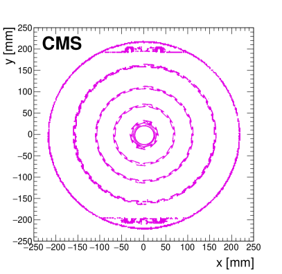
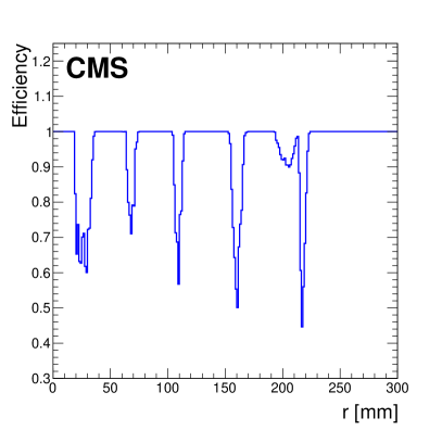
Figure 2: Left: the NI-veto map based on the NI vertex reconstruction in the 2017 and 2018 data collected by the CMS detector, the map corresponds to the geometry of the CMS pixel detector used in 2017–2018 data taking [CMS:2012sda]. The structures of the different pixel layers can be clearly seen. Right: the efficiency for a given vertex candidate to pass the NI-veto as a function of radius $r$.

The preselection criteria for this search, summarized in Table 0.4, are efficient for a wide range of long-lived models with different final-state topologies.

Summary of the preselection criteria. lc SV/dijet variable & Requirement
Vertex $\chi^{2}/\mathrm{n_{dof}}$ $<$5.0
Vertex invariant mass $>$$4\GeV$
Vertex transverse momentum $>$$8\GeV$
Second largest $\mathrm{IP_{2D}}$ significance $>$15
$\epsilon$ (SV track energy fraction in the dijet) $>$0.15
$\zeta$ (energy fraction from compatible PVs) $<$0.20
Vertex position in the $x$-$y$ plane no overlap with the NI-veto map

0.5 Event selection and background prediction

After reconstructing the SV using the adaptive vertex fitter, we employ an auxiliary algorithm to check the consistency between the SV system and the dijet system. For each displaced track (having $\mathrm{IP_{2D}}>0.5\mm$, $\mathrm{Sig[IP_{2D}]}>5.0$) associated with the dijet, we determine an expected decay point consistent with the displaced dijet hypothesis by finding the crossing point of the track helix and the dijet direction in the transverse ($x$-$y$) plane. The dijet direction is the space direction of the four-momentum-sum of the two jets, for which the production vertex of the two jets is taken to be the SV. For each crossing point, an expected transverse decay length ($L_{xy}^{\mathrm{exp}}$) is computed with respect to the leading PV. The $L_{xy}^{\mathrm{exp}}$ is positive if the crossing point is at the same side of the dijet direction, otherwise it is negative. The associated displaced tracks are then clustered based on their $L_{xy}^{\mathrm{exp}}$, using a hierarchical clustering algorithm [Johnson1967]. During the clustering, two clusters are merged when the smallest $L_{xy}^{\mathrm{exp}}$ difference between the two clusters is smaller than $15\%$ of the $L_{xy}$ of the SV. After the clustering procedure is finished, if more than one cluster is formed, the one closest to the SV is selected. The cluster root-mean-square (RMS), taken to be the relative RMS of individual tracks $L_{xy}^{\mathrm{exp}}$ with respect to the SV $L_{xy}$, is computed to provide signal-to-background discrimination:

$$\mathrm{RMS}_{\mathrm{cluster}}=\sqrt{\frac{1}{N_{\mathrm{tracks}}}\sum_{i=1}^{N_{\mathrm{tracks}}}\frac{(L_{xy}^{\mathrm{exp}}(i)-L_{xy})^{2}}{L_{xy}^{2}}},$$ (3)

where $N_{\mathrm{tracks}}$ is the number of tracks in the selected cluster.

For each track assigned to the SV, a sign is given to the $\mathrm{IP_{2D}}$ and $\mathrm{Sig[IP_{2D}]}$ based on the angle between the dijet direction and the impact parameter vector that points from the leading PV to the closest approach point (with respect to the leading PV) of the track in the transverse plane. The sign is positive if this angle is smaller than $\pi/2$; otherwise the sign is negative. A new variable, $\kappa$, is then introduced as the signed $\mathrm{Sig[IP_{2D}]}$ sum of the six leading tracks from the SV (where the tracks are ordered by the absolute values of their $\mathrm{Sig[IP_{2D}]}$):

$$\kappa=\sum_{i=1}^{6}\mathrm{Sig[IP_{2D}(track_{\emph{i}})]}.$$ (4)

If the track multiplicity is smaller than six, the sum is taken over all the tracks from the SV. For background processes, since the tracks assigned to the SV are uncorrelated with the dijet direction, the signed $\mathrm{Sig[IP_{2D}]}$ of different tracks tend to cancel each other, therefore $\kappa$ peaks sharply around zero. On the other hand, for displaced jets that originate from the SV, the directions of the tracks will be highly correlated with the dijet direction, therefore $\kappa$ is significantly different from zero and $\abs{\kappa}$ tends to be large.

To improve signal-to-background discrimination and to define a region with signal events enriched, we proceed to construct a multivariate discriminant based on the following variables for the vertex/dijet candidates:

• Vertex track multiplicity;

• Vertex $L_{xy}$ significance;

• Cluster RMS;

• The magnitude of the signed $\mathrm{Sig[IP_{2D}]}$ sum of the six leading tracks $\abs{\kappa}$.

The distributions of the four variables are shown in Fig. 3, with displaced-jet triggers, offline , and offline jet kinematic variables selections (described in Section 0.4) applied. For the multivariate discriminant we utilize the gradient boosted decision tree (GBDT) algorithm [Freund:1996:ENB:3091696.3091715, friedman2000, friedman2001], with cross entropy as the loss function. The GBDT algorithm is implemented using the TMVA (toolkit for multivariate data analysis) package [Hocker:2007ht] interfaced with Scikit-learn [Pedregosa:2011:SML:1953048.2078195]. Given the large cross section of the QCD multijet process and the relatively low threshold of our displaced-jet triggers, the event count of the simulated QCD multijet sample (after preselections) is insufficient for the GBDT training, since it is much smaller than the number of expected QCD multijet events in the analyzed data sample. Therefore, for the background sample in the GBDT training, we use the data in the following region:

• events are selected by the displaced-jet triggers, and pass the offline and jet kinematic variables selections;

• $\epsilon<0.12$ for the dijet candidate, making this region orthogonal to the signal region;

• the veto using the NI-veto map is not applied;

• all the other preselection criteria are satisfied.

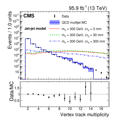
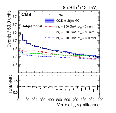
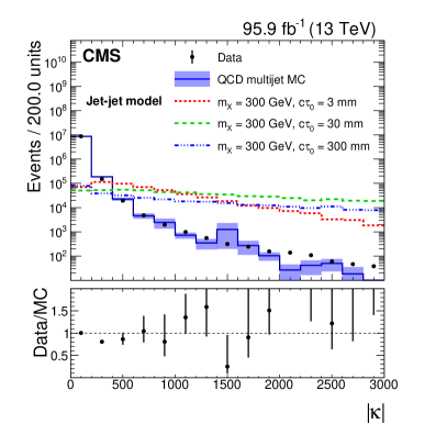
Figure 3: The distributions of the vertex track multiplicity (upper left), vertex $L_{xy}$ significance (upper right), cluster RMS (lower left), and the magnitude of the signed $\mathrm{Sig[IP_{2D}]}$ sum $\abs{\kappa}$ (lower right), for data, simulated QCD multijet events, and simulated signal events. Data and simulated events are selected with the displaced-jet triggers and with the offline , jets , and $\eta$ selections applied. For a given event, if there is more than one SV candidate being reconstructed, the one with the largest vertex track multiplicity is chosen. If the track multiplicities are the same, the one with the smallest $\chi^{2}/\mathrm{n_{dof}}$ is chosen. The lower panels show the ratios between the data and the simulated QCD multijet events. The blue shaded error bands and vertical bars represent the statistical uncertainties. Three benchmark signal distributions are shown (dashed lines) for the jet-jet model with $m_{\mathrm{X}}=300\GeV$ and varying $c\tau_{0}$. For visualization purposes, each signal process is given a cross section that yields $10^{6}$ events produced in the analyzed data sample.

For the signal sample in the GBDT training, simulated jet-jet model events that pass the preselection criteria are used, with $m_{\mathrm{X}}=100$, 300, and 1000, and with $c\tau_{0}=1$, 10, 100, 1000. If there is more than one dijet/SV candidate passing the selection criteria in a given event, the one with the largest track multiplicity is chosen for the training. If the track multiplicities are the same, the one with the smallest SV $\chi^{2}/\mathrm{n_{dof}}$ is chosen. An event weight is assigned separately to each signal point with a given $m_{\mathrm{X}}$ and $c\tau_{0}$ such that the sum of weights is identical for each point, thus each signal point has the same priority in the training. Twenty percent of the events in the signal and background samples are randomly selected to validate the performance of the GBDT and to make sure it is not overtrained.

The GBDT output values or scores for data, simulated QCD multijet events, and simulated signal events are shown in Fig. 4. The signal efficiencies for this search are measured with simulated signal events produced separately. The background prediction is purely based on some other control samples in data, which are different from the one used for the GBDT training. Although only the jet-jet model is used as the signal sample in the GBDT training, the GBDT is highly efficient in selecting signatures of other LLP models with different final-state topologies, since we have explicitly chosen the input variables to make the GBDT as model-independent as possible.

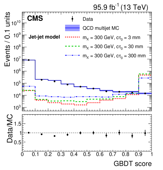
Figure 4: The distributions of the GBDT output score for data, simulated QCD multijet events, and simulated signal events. Data and simulated events are selected with the displaced-jet triggers and with the offline , jets , and $\eta$ selections applied. For a given event, if there is more than one SV candidate being reconstructed, the one with the largest vertex track multiplicity is chosen. If the track multiplicities are the same, the one with the smallest $\chi^{2}/\mathrm{n_{dof}}$ is chosen. The lower panel shows the ratio between the data and the simulated QCD multijet events. The blue shaded error bands and vertical bars represent the statistical uncertainties. Three benchmark signal distributions are shown (dashed lines) for the jet-jet model with $m_{\mathrm{X}}=300\GeV$ and varying $c\tau_{0}$. For visualization purposes, each signal process is given a cross section corresponding to $10^{6}$ events produced in the analyzed data sample. The signal events shown in this plot are not used in the GBDT training.

In addition to the GBDT score $g$, we use another variable $N_{\mathrm{tracks}}^{\mathrm{3D}}$ in the final event selection, which is the number of 3D prompt tracks in a single jet, where the 3D prompt tracks are the tracks that have 3D impact parameters with respect to the leading PV smaller than 0.3.

If more than one dijet candidate passes the preselection criteria described in Section 0.4, the one with the largest GBDT score is selected. If the GBDT scores are the same, the one with the smallest SV $\chi^{2}/\mathrm{n_{dof}}$ is selected. In the final signal region, the candidate is further required to pass three final selection criteria, which are:

• Selection 1: for the leading jet in , $N_{\mathrm{tracks}}^{\mathrm{3D}}$ is smaller than 3;

• Selection 2: for the subleading jet, $N_{\mathrm{tracks}}^{\mathrm{3D}}$ is smaller than 3; and

• Selection 3: the GBDT score $g$ is larger than 0.988.

The numerical values for the selection criteria are chosen by optimizing the discovery potential of 5 standard deviations based on the Punzi significance [Punzi:2003bu] for the jet-jet model and the $\sGlu\to\Glu\sGra$ model across different LLP masses and lifetimes. The chosen models encompass the displaced-dijet and displaced-single-jet signatures, with $m_{\mathrm{X}}=100$, 300, and 1000for the jet-jet model, and with $m_{\sGlu}=600$, 1000, and 1600for the $\sGlu\to\Glu\sGra$ model, while $c\tau_{0}$ is taken to be 1, 10, 100, and 1000. Thus there are 24 signal points considered in total for the selection optimization.

Based on the three selection criteria, we can define eight nonoverlapping regions A–H, which include the final signal region. The event counts in different regions are $N_{fff}$, $N_{pff}$, $\cdots$, and $N_{ppp}$, for regions A, B, $\cdots$, and H, respectively, as shown in Table 0.5. The region H is the region where the events pass all the three selection criteria, and thus is the final signal region. Events in the remaining regions (A–G) fail one or more of the three selection criteria. Since the three selection criteria have little correlation between them for the background events, a property that has been verified with simulated QCD multijet events, the background yield in the signal region H can be estimated by different ratios of event counts in regions A–G, where the ratio $b_{\mathrm{nominal}}=N_{ppf}(N_{ffp}+N_{fpp}+N_{pfp})/(N_{fff}+N_{pff}+N_{fpf})$ uses the fraction of events passing to those failing the GBDT selection (Selection 3) and is taken as the central value of the predicted background yields. Three additional ratios are computed using the events failing either one of the first two selections:

• Cross-check 1: $N_{ppf}(N_{ffp}+N_{fpp})/(N_{fff}+N_{fpf})$;

• Cross-check 2: $N_{ppf}(N_{ffp}+N_{pfp})/(N_{fff}+N_{pff})$;

• Cross-check 3: $N_{ppf}(N_{fpp}+N_{pfp})/(N_{fpf}+N_{pff})$.

The definitions of the different regions used in the background estimation. ccccc Region Selection 1 Selection 2 Selection 3 Event count
A Fail Fail Fail $N_{fff}$
B Pass Fail Fail $N_{pff}$
C Fail Pass Fail $N_{fpf}$
D Fail Fail Pass $N_{ffp}$
E Fail Pass Pass $N_{fpp}$
F Pass Fail Pass $N_{pfp}$
G Pass Pass Fail $N_{ppf}$
H Pass Pass Pass $N_{ppp}$

These cross-checks provide an important test of the robustness of the background prediction and the assumption that the three selection criteria are minimally correlated. Differences between the predictions obtained with the nominal ratio $b_{\mathrm{nominal}}$ and the cross-checks are used to estimate the systematic uncertainties in the background prediction.

The method described above can be generalized to predict the background yield in arbitrary intervals of the GBDT score $g$, where the first two selections are also satisfied. In this way we can verify our background prediction method in the different bins of GBDT score $g$. The background prediction method is first tested with simulated QCD multijet events and simulated signal events, and is found to be robust both with and without signal contaminations. We then test the background prediction in data, for which we define a control region by inverting the selection on $\epsilon$, requiring $\epsilon$ to be smaller than 0.15. In order to improve the statistical precision, we remove the selection requirement that uses the NI-veto map, although the background prediction method is still robust with the presence of the NI-veto map. The predicted background yields and observed events in the control region are shown in Fig. 5, which shows a good agreement between the predicted and observed yields. The predicted background yields in the different bins of GBDT score are correlated, since the events that are used for background predictions in lower bins are also used in the background predictions in higher bins.

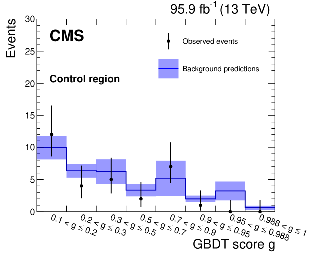
Figure 5: The predicted background yields and the numbers of observed events in the control region, for different bins of the GBDT scores. The background predictions in different bins are correlated, since the events that are used for background predictions in lower bins are also used in the background predictions in higher bins. The error bands for the predictions represent statistical uncertainties and systematic uncertainties added in quadrature. The error bars for the observed events represent statistical uncertainties, assuming Poisson statistics.

0.6 Systematic uncertainties

The systematic uncertainty in the background prediction is taken to be the largest deviation of the three cross checks from the nominal prediction $b_{\mathrm{nominal}}$, and is found to be 52% in the final signal region where the GBDT score $g$ is larger than 0.988.

The systematic uncertainties in the integrated luminosity for 13$\Pp\Pp$ collision data are 2.3% and 2.5% for the 2017 and 2018 [CMS:2018elu, CMS:2019jhq] data taking periods, respectively, and are modeled as uncorrelated nuisance parameters between the years.

The systematic uncertainty in the signal yields arising from the pileup modeling is estimated by varying the inelastic $\Pp\Pp$ cross section [Sirunyan:2018nqx] used in the pileup distribution determination by 4.6%. The resulting variations of the signal yields are generally smaller than 1% and are well within the statistical fluctuations, therefore the impact of the pileup modeling is negligible and no corresponding systematic uncertainty is assigned.

The systematic uncertainty in the signal yields due to the online requirements of the displaced-jet triggers is estimated by comparing the efficiency of the online requirements measured in data with the one measured in the QCD multijet MC sample. The efficiencies are measured using the events collected with an isolated single-muon trigger. The discrepancies between the measurements in data and MC simulation are parameterized as functions of offline , and corresponding corrections are applied to the simulated signal events. The signal yields are then recalculated for different masses and mean proper decay lengths. The largest correction in the signal yield for a given model is taken as the corresponding systematic uncertainty, and is found to be smaller than 2%.

The systematic uncertainty in the signal yields due to the online jet requirements of the displaced-jet triggers is estimated by measuring the per-jet efficiencies of the online jet requirements in data and in the QCD multijet MC sample, using events collected with a prescaled trigger that requires $\HT>425\GeV$. Corrections for the discrepancies between the measurements in data and MC simulation are applied to the simulated signal events, and the signal yields are recalculated. The correction is more significant for low-mass LLPs (with $m\sim 50\GeV$), and is smaller than 8%, which is taken as the corresponding systematic uncertainty.

To estimate the systematic uncertainty due to the online tracking requirements of the displaced-jet triggers, we measure the per-jet efficiencies of the online tracking requirements as functions of the number of prompt tracks and displaced tracks, using events collected with the prescaled trigger. The efficiencies obtained in data are found to be consistent with the efficiencies obtained in MC simulations. Therefore no corresponding systematic uncertainty is assigned.

To estimate the impact of the possible mismodeling of the GBDT score in MC simulation on the signal yields, we compare the distribution of the GBDT score in simulated QCD multijet events with the distribution measured in data, using events collected with the prescaled trigger. The discrepancies between data and MC simulation are taken into account by varying the GBDT scores in the simulated samples by the same magnitude. The largest variation in the signal efficiency for a given model is taken as the corresponding systematic uncertainty in signal yields, and is found to be in the range of 4%–15%.

Similarly, the uncertainty in the signal yields due to impact parameter modeling is estimated by comparing the distribution of the impact parameters in simulated QCD multijet events with the distribution measured in data, also using events collected with the prescaled trigger. The impact parameters in simulated QCD multijet events are varied until the discrepancies between data and MC simulation are covered by the variation. The impact parameters in the simulated signal samples are then varied by the same magnitude. The largest variation in the signal efficiency for a given model is taken as the corresponding systematic uncertainty, and is found to be in the range of 8%–18%.

The impact of the jet energy scale uncertainty on the signal yields is estimated by varying the jet energy and by one standard deviation of the jet energy scale uncertainty [Khachatryan:2016kdb]. The variations of the signal efficiencies are smaller than 3%, which is taken as the corresponding systematic uncertainty.

The impact of the PDF uncertainty on the signal acceptance is estimated by reweighting the simulated signal events with NNPDF, CT14 [Dulat:2015mca] and MMHT14 [Harland-Lang:2014zoa] PDF sets, and their associated uncertainty sets [Butterworth:2015oua, Buckley:2014ana], following the PDF4LHC recommendation [Butterworth:2015oua]. The uncertainty in signal efficiency for a given signal model is quantified by comparing the efficiencies calculated with alternative PDF sets and the ones with the nominal NNPDF set, and is found to be in the range of 4–6%.

The uncertainty in the signal yields due to the selection of the PV is estimated by replacing the leading PV with the subleading PV when calculating impact parameters and vertex displacement. The largest variation of the signal efficiency for a given signal model is taken as the corresponding systematic uncertainty, and is found to be in the range of 8–15%.

The various systematic uncertainties in the signal yields are summarized in Table 0.6.

Summary of the systematic uncertainties in the signal yields. lc Source Uncertainties (%)
Integrated luminosity 2.3–2.5
Online requirement 0–2
Online jet requirement 0–8
Offline vertexing 4–15
Track impact parameter modeling 8–18
Jet energy scale 0–3
PDF 4–6
Primary vertex selection 8–15
Total 17–25