Single-top-quark production in the $t$-channel at NNLO

Abstract

We present a calculation of $t$-channel single-top-quark production and decay in the five-flavor scheme at NNLO. Our results resolve a disagreement between two previous calculations of this process that found a difference in the inclusive cross section at the level of the NNLO coefficient itself. We compare in detail with the previous calculations at the inclusive, differential and fiducial level including $b$-quark tagging at a fixed scale $\mu=m_{t}$. In addition, we advocate the use of double deep inelastic scattering (DDIS) scales ($\mu^{2}=Q^{2}$ for the light-quark line and $\mu^{2}=Q^{2}+m_{t}^{2}$ for the heavy-quark line) that maximize perturbative stability and allow for robust scale uncertainties. All NNLO and $\text{NLO}{}\otimes\text{NLO}{}$ contributions for production and decay are included in the on-shell and vertex-function approximation. We present fiducial and differential results for a variety of observables used in Standard Model and Beyond Standard Model analyses, and find an important difference between the NLO and NNLO predictions of exclusive $t+n$-jet cross sections. Overall we find that NNLO corrections are crucial for a precise identification of the $t$-channel process.

1 Introduction

Top quarks play a special role in the Standard Model (SM). They stand out from the other quarks by virtue of their mass, significantly larger than their peers, and by the fact that they decay before they are able to form bound states. The former property ensures that top quarks are primarily responsible for the production of Higgs bosons at hadron colliders, by mediating the loop-induced coupling $gg\to h$, and positions them as potential portals to so-far undiscovered extensions of the SM. The latter enables both a clean theoretical description of top-quark processes and, on the experimental side, their identification through decays into well-measured objects. Therefore the study of the production and decay of top quarks is a cornerstone of the current and future physics program of the Large Hadron Collider (LHC).

The primary mechanism for producing top quarks is through the strong interaction, resulting in the creation of a top quark-antiquark pair. However, a single top quark may also be produced through a weak interaction involving a bottom quark. In fact, the $t$-channel single top production processes, represented at leading order by,

$$q+\overset{(-)}{b}\to q^{\prime}+\overset{(-)}{t}\,,$$ (1)

and first observed at the Tevatron [1, 2], are responsible for approximately $20\%$ of all top-quark production at the LHC. Despite this production mode proceeding through weak couplings, the rate is large due to its $t$-channel nature and the fact that it is kinematically favored compared to the pair-production process. The channel of course provides a useful probe of the top quark itself, with measurements of the top-quark mass [3] and polarization [4], detailed tests of the Standard Model at the differential level [5, 6], as well as constraints on anomalous $Wtb$ couplings [7, 8, 9]. In addition, it can also provide valuable information on the elements of the production mechanism: the bottom quark parton distribution function (PDF) and the CKM matrix element, $V_{tb}$. Indeed, measurements of $V_{tb}$ have been made at both the Tevatron [10] and the LHC [11, 12, 13, 14].

In order to turn experimental observations into precision measurements it is essential to have theoretical calculations with small residual uncertainties. One of the largest sources of theoretical uncertainty results from the truncation of the perturbative expansion at a fixed order and is usually estimated by scale variation. Generically, this scale variation is expected to decrease order-by-order, with percent-level uncertainties only expected when going to the current gold-standard for precision measurements, next-to-next-to-leading order (NNLO). For top-quark processes another consideration that complicates the perturbative calculation stems from the fact that the top quark decays, $t\to W^{+}b$. Accounting for such a decay, at leading order, does not present a tremendous complication – in fact, using the spinor helicity approach, expressions for relevant matrix elements are extremely compact [15]. However, once strong-coupling corrections are included one should, in principle, account for the effects of virtual radiation that connects strongly-interacting particles in the ‘production’ and ‘decay’ elements of the process.

The earliest results for $t$-channel single top production that included corrections to next-to-leading order (NLO) in the strong coupling were computed for a stable top quark, that is, for exactly the processes shown in eq. 1 [16, 17, 18]. These were soon extended beyond the case of the inclusive cross section, to also describe fully-differential measurements of this process [19, 20, 21]. Somewhat later the decay of the top quark was also included at the same order, with calculations performed in a factorized approach in which the top quark remains on its mass shell and radiation that connects production and decay is neglected [22, 23, 24]. Although this is an inherent approximation, for sufficiently inclusive observables such off-shell effects are small, of the order of $\Gamma_{t}/m_{t}$ [25, 26]. For a precision prediction of the invariant mass of the top quark it is clearly essential to move away from this approximation and, in general, more differentially such effects are of increasing importance. Calculations of off-shell effects were first performed in an effective field theory approach, valid in the region of the resonance [27, 28, 29, 30], and subsequently computed exactly [31, 32, 33].

The first steps towards including the effects of NNLO corrections to this process were taken in refs. [34, 35], in which the top-quark decay was computed at this order. The corresponding NNLO corrections for the hadroproduction of a stable top quark in this channel were subsequently computed [36] and, finally, the full corrections in both the production and decay stages were included in the calculation presented in refs. [37, 38]. The results of these calculations indicate that, at the inclusive level, the effect of the NNLO corrections is small, leading to a change in the cross section of only a few percent. However, the effects of the corrections can be larger in the fiducial volume [37, 38]. Importantly, a comparison between the two groups – at the level of inclusive cross sections for a stable top quark – revealed that the two calculations disagree at the 1% level [37], that is, at almost the same level as the effect of the NNLO corrections themselves. Recently, the NNLO calculation of refs. [37, 38] has been used to study the top-quark mass determination [39] and differences between flavor schemes [40].

The importance of this production mode demands that the existing theoretical calculations be scrutinized, cross-checked and any discrepancies understood. To this end, in this paper we present a full re-calculation of the NNLO QCD corrections to this process, including all the effects of radiation in top-quark production and decay at this order. Although the calculation necessarily shares some elements and methodology with previous work, it has been performed from scratch from ingredients that have been, where possible, verified against independent computations. In order to ensure the maximum value of the calculation, it is performed using the framework of the MCFM package [41, 42, 43] and will be distributed publicly. The aim of this approach is to ensure that the latest possible theoretical information can always be incorporated in future experimental analyses, incorporating any demands on input parameters such as the top-quark mass and PDFs.

The outline of the paper is as follows. In section 2 we describe the setup of our calculation: outlining the general structure, discussing the role of a strict fixed-order expansion that becomes relevant when including the top-quark decay and introducing the distinctive choice of factorization and renormalization scales for this process. We also describe our prescription for $b$-quark tagging, which at NNLO needs special attention. We then present details of all the necessary ingredients for the three independent NNLO sub-calculations entering our results, as well as of the $\text{NLO}{}\otimes\text{NLO}{}$ interference contributions, and describe the checks that we have performed to validate our results. In section 3 we compare in-depth with the previous stable-top calculation and the on-shell calculation with decay. Last, in section 4 we discuss fully inclusive cross sections, cross sections with fiducial cuts, and the relevant differential distributions used in experimental analyses. We furthermore consider NNLO results for angular observables in the top-quark rest frame, angles that are used for searches of physics beyond the Standard Model and which are sensitive to $Wtb$-vertex modifications in the production and decay stages.

2 Calculation

Our calculation of NNLO QCD corrections to $t$-channel single-top-quark production and decay is performed in the five-flavor scheme, a $2\to 4$ scattering process at Born level that is depicted schematically in fig. 1. In order to render the calculation tractable we perform the calculation in the on-shell approximation, neglecting contributions from radiation that connects the production and decay stages such as the diagram shown in fig. 2 (left). For a large class of observables this amounts to discarding off-shell effects that are of order $\Gamma_{t}/m_{t}$ [25, 26]. We furthermore neglect a class of two-loop box diagrams that connect the light-quark and heavy-quark lines, that are suppressed by a color factor of $1/N_{c}^{2}$, see fig. 2 (right). The NNLO corrections therefore consist of NNLO vertex corrections on the light-quark line and the heavy-quark line in the production part of the process, as well as NNLO vertex corrections in the decay of the top quark, as indicate in fig. 1. In the literature this is also known as the structure function approximation. Of course, in addition to second-order corrections to each vertex, at NNLO we must also include one-loop times one-loop interference contributions.

Figure 1: Feynman diagram for $t$-channel production in the on-shell approximation with blobs denoting vertex corrections on the light line (L), on the heavy line in production (H) and in decay (D).

Figure 2: Example Feynman diagrams for one-loop off-shell contributions (left) and color-suppressed interference contributions (right) in $t$-channel production.

We calculate each of the three NNLO vertex corrections in fig. 1 using slicing-based subtractions derived from different factorization theorems. The interference contributions are calculated in a mixed slicing-dipole subtraction scheme. While we use the same NNLO factorization theorem to assemble the corrections on the heavy line in production and decay as in a previous calculation [37, 38], we have performed a series of exhaustive analytical and numerical checks to ensure a correct cancellation of IR divergences between all amplitudes. Our implementation of each contribution is, of course, completely independent and all amplitudes have either been calculated from scratch or obtained from different sources. With this we can guarantee a fully independent cross-check of previous results. The calculational details for the three NNLO vertex corrections and the $\text{NLO}{}\otimes\text{NLO}{}$ interference are given in the next four subsections, but we first discuss some general aspects of the calculation.

Fixed-order expansion.

Since the top quark can be treated as a quasi-stable particle to a good approximation, the differential cross section $\mathrm{d}\sigma(\alpha_{s})$ can be factorized into a production part $\mathrm{d}\sigma^{\text{production}}(\alpha_{s})$ and a decay part $\mathrm{d}\Gamma_{t}(\alpha_{s})/\Gamma_{t}(\alpha_{s})$. In the decay corrections the numerator is the differential decay width and the denominator is its integrated expression, such that the integration of the decay fully inclusively leads to no change in the cross section. Throughout this paper we assume that the top-quark decays 100% of the time to a $W$ boson and a $b$ quark.

While it is possible to keep the full expression of the width in the denominator, it is customary to expand the whole cross section $\mathrm{d}\sigma(\alpha_{s})$ in $\alpha_{s}$ to avoid higher-order contributions from the expansion of the width in the denominator and the factorized contributions of the individual vertex corrections. Consequently, we expand the fully differential cross section $\mathrm{d}\sigma(\alpha_{s})=\mathrm{d}\sigma^{\text{production}}(\alpha_{s})\otimes\mathrm{d}\Gamma_{t}(\alpha_{s})/\Gamma_{t}(\alpha_{s})$ consistently in $\alpha_{s}$ to obtain cross sections at LO ($\alpha_{s}^{0}$), NLO ($\alpha_{s}$) and NNLO ($\alpha_{s}^{2}$). The symbol $\otimes$ denotes that production and decay are taken fully at the amplitude level including all spin correlations. Denoting with $\mathrm{d}\sigma^{(j)}$ the contribution of order $\alpha_{s}^{j}$ in production and with $\mathrm{d}\Gamma_{t}^{(k)}$ the contribution of order $\alpha_{s}^{k}$ in decay, the fixed-order expansion is explicitly given by:

$$\begin{split}\mathrm{d}\sigma_{\text{LO}}{}&=\frac{1}{\Gamma_{t}^{(0)}}\mathrm{d}\sigma^{(0)}\otimes\mathrm{d}\Gamma_{t}^{(0)}\,,\\ \mathrm{d}\sigma_{\delta\text{NLO}{}}&=\frac{1}{\Gamma_{t}^{(0)}}\Bigg{[}\mathrm{d}\sigma^{(1)}\otimes\mathrm{d}\Gamma_{t}^{(0)}+\mathrm{d}\sigma^{(0)}\otimes\left(\mathrm{d}\Gamma_{t}^{(1)}-\frac{\Gamma_{t}^{(1)}}{\Gamma_{t}^{(0)}}\mathrm{d}\Gamma_{t}^{(0)}\right)\Bigg{]}\,,\\ \mathrm{d}\sigma_{\delta\text{NNLO}{}}&=\frac{1}{\Gamma_{t}^{(0)}}\Bigg{[}\mathrm{d}\sigma^{(2)}\otimes\mathrm{d}\Gamma_{t}^{(0)}+\mathrm{d}\sigma^{(1)}\otimes\left(\mathrm{d}\Gamma_{t}^{(1)}-\frac{\Gamma_{t}^{(1)}}{\Gamma_{t}^{(0)}}\mathrm{d}\Gamma_{t}^{(0)}\right)\\ &\qquad\qquad+\mathrm{d}\sigma^{(0)}\otimes\left(\mathrm{d}\Gamma_{t}^{(2)}-\frac{\Gamma_{t}^{(2)}}{\Gamma_{t}^{(0)}}\mathrm{d}\Gamma_{t}^{(0)}-\frac{\Gamma_{t}^{(1)}}{\Gamma_{t}^{(0)}}\left(\mathrm{d}\Gamma_{t}^{(1)}-\frac{\Gamma_{t}^{(1)}}{\Gamma_{t}^{(0)}}\mathrm{d}\Gamma_{t}^{(0)}\right)\right)\Bigg{]}\,,\end{split}$$ (2)

where $\Gamma_{t}^{(l)}$ are the integrated decay corrections of order $\alpha_{s}^{k}$. By construction, the expressions in parentheses vanish upon fully inclusive integration over the decay

Double deep inelastic scattering (DDIS) scales.

Our implementation allows for different factorization and renormalization scales in light-line corrections, heavy-line corrections in production, and corrections in decay. For our approximation in terms of vertex corrections the natural choice to minimize scale-dependent logarithms for fully inclusive results is to take $Q^{2}$ as the central scale on the light-quark line, $Q^{2}+m_{t}^{2}$ on the heavy-quark line in production, and $m_{t}$ in the decay, where $Q^{2}$ is the positive squared momentum of the $W$ boson. We abbreviate this set of scale choices as DDIS (double deep inelastic scattering) scales.

The motivation for considering DDIS scales stems from the observation that single-top-quark production in our approximation is double deep inelastic scattering with a light and heavy quark. When PDFs are extracted from DIS measurements, one therefore expects our perturbative results to be stable across orders with DDIS scales. That is, strictly speaking, the cross sections at LO, NLO and NNLO should agree within PDF uncertainties. Therefore, at least in principle, using DDIS scales can be exploited as a constraint for PDFs. At NNLO, off-shell effects and color-suppressed contributions from two-loop box diagrams break this property, see fig. 2, but such effects are estimated to be small, at least inclusively.

$b$-quark tagging.

Tagging a specific quark flavor in jets, say a $b$ quark, raises the question of infrared safety. Throughout NLO there are no issues, but at NNLO a large-angle soft gluon splitting $g\to b\bar{b}$ can lead to $b$-quarks being clustered into different jets, violating flavor infrared safety. Typical jet algorithms only ensure infrared safety at the event momentum level, and this situation breaks infrared safety at the jet flavor level. A general solution is to employ a flavor-jet algorithm for infrared-safe predictions [45, 46], which ensures that such a soft splitting would recombine to a flavorless jet.

Experimentally such a flavor-jet algorithm is not used in single-top-quark analyses and we do not adopt such an algorithm in this study. Although it could, in principle, be interesting to consider its impact in the future, the difference is likely to be negligible due to the smallness of the $g\to b\bar{b}$ contributions, see below. For now we adopt the strategy used in ref. [38], which also enables a more transparent comparison with the results presented in that reference. The procedure is as follows: for the NNLO vertex corrections in production the $g\to b\bar{b}$ splitting does not come with another $b$ quark at the same vertex. The flavor in the pair can therefore be ignored on the premise that it gives a tiny contribution. In the decay the situation with an additional $b$ quark from the top-quark decay arises and the flavor is ignored for the $b\bar{b}$ pair with the smaller invariant mass, which is most likely the pair originating from the $g\to b\bar{b}$ splitting.

The authors of ref. [38] check the infrared safety of this approach numerically by evaluating the infrared subtraction slicing-cutoff dependence. They find that when no flavors are ignored there is indeed a difference, but it is tiny. We do confirm these findings, and note that the minuscule size of this effect, unless one probes tiny slicing cutoffs to enhance it, confirms that the flavor contribution of the $g\to b\bar{b}$ contribution is negligible. Therefore, using a full flavor-jet algorithm does not seem necessary in practice.

We furthermore adopt the following choice of the $b$-jet definition for the remainder of this paper. Namely, we define the $b$-number of a jet to be the sum of the $b$-numbers of its constituent partons, where the $b$-number of a $b$ and $\bar{b}$ quark are $+1$ and $-1$, respectively. A jet with non-zero $b$-number is termed a $b$-jet and all other jets are light jets.

Common ingredients.

Before detailing the individual NNLO calculations, we first summarize some ingredients shared by all parts. For the calculation of the NNLO vertex corrections, the above-cut slicing contributions are obtained by performing NLO calculations of partonic processes corresponding to Born configurations plus an additional parton. Importantly, these have to be numerically stable in the doubly-singular limits. The necessary tree-level and one-loop amplitudes for these calculations are assembled from existing amplitudes in MCFM for one-loop corrections [22] and tree-level results in the four-flavor scheme [47]. We use dipole subtractions to combine them into NLO calculations for massless [48] and massive [49] particles. The extension to limit the size of subtractions provides an additional check of a correct implementation (“alpha independence”) and can improve numerical stability. These extensions have been worked out for both massless [50, 51] and massive [22, 52, 53] partons. Note that to retain a proper definition of the DDIS scales, the dipoles in our NLO calculations must be chosen with some care so that no initial-initial dipoles transform momenta on both lines.

2.1 Top-quark-production corrections on the light line

For the light-quark line, which represents DIS-like jet production, we compute the NNLO corrections using a factorization theorem in the 1-jettiness variable $\tau_{l}$ for massless partons [54]. This approach has been first used in ref. [55] for a calculation of $W$+jet at NNLO and the formalism including all necessary ingredients at NLO has been presented in full generality in ref. [56].

At NNLO we have to take into account contributions with one and two extra emissions in addition to the parton already present at Born level. We denote with $M$ the number of (light-line) partonic emissions $p_{k}^{\mu}$, $k=1,\ldots,M$ and the initial state light-quark (beam) momentum as $q_{b}$. Then our 1-jettiness variable is defined as

$$\tau_{l}=\frac{1}{Q_{0}}\sum_{k=1}^{M}\min\{n_{b}p_{k},n_{j}p_{k}\}\,$$ (3)

where $n_{b}$ is the normalized beam direction $q_{b}^{\mu}$ and $n_{j}$ is a normalized jet direction. The scale $Q_{0}$ is introduced to make $\tau_{l}$ dimensionless, as discussed further below. Obtaining the jet direction $n_{j}$ from an explicit minimization of $\tau_{l}$ for one and two additional emissions has been discussed in refs. [56, 54]. For example for $M=2$ the result is

$$\tau_{l}=\frac{1}{Q_{0}}\min\left\{\min\{E_{1}-p_{1}^{z},E_{2}-p_{2}^{z}\},\,E_{1}+E_{2}-|\vec{p}_{1}+\vec{p}_{2}|\right\}\,,$$ (4)

effectively partitioning the phase space into extra emission clustered with the beam, or together with the other final state emission. Here $p_{k}^{z}$ is the $z$-component of $p_{k}^{\mu}$, $E_{k}$ is the energy of $p_{k}^{\mu}$, and $\vec{p}_{k}$ is the spatial component of $p_{k}^{\mu}$. The case of $M=3$ results in a similar partitioning, where now all extra emissions can either be together, or with the beam, or one with the beam and one with the other emission, in various combinations. For further details, see ref. [56] or our implementation in MCFM.

For the plots presented in this study we choose $Q_{0}=$1\text{\,}\mathrm{GeV}$$. An alternative choice is $Q_{0}\propto\sqrt{Q^{2}}$, where $Q^{2}$ is the squared $W$ boson momentum transfer. We find that at $\sqrt{s}=$13\text{\,}\mathrm{TeV}$$ the choice of $Q_{0}\sim\sqrt{Q^{2}}/100$ has similar numerical stability as $Q_{0}=$1\text{\,}\mathrm{GeV}$$ and is subject to power corrections that are of the same magnitude, as may be anticipated from the explicit minimization indicated in eq. 4. We do not explore this difference any further here.

Instead of the explicit minimization of $\tau_{l}$, in principle any infrared-safe Born projection can be used to obtain the jet axis $n_{j}$. For example one could determine it from the jet clustering algorithm, as has previously been done in MCFM. Any difference in the Born projection results in different power-suppressed terms in the factorization theorem, but does not modify its singular structure [54].

With this phase-space partitioning, one can write down the $1$-jettiness factorization theorem integrated over $\tau_{l}$ as a subtraction scheme as

$$\mathrm{d}\sigma_{a,b}(\tau_{l}<\tau_{l}^{\text{cut}})=\mathrm{d}\sigma^{\text{Born}}\,f_{b}(x_{b},\mu)\int_{0}^{\tau_{l}^{\text{cut}}}\!\!\!\mathrm{d}\tau_{l}^{\prime}\int\!\mathrm{d}k_{j}\int\!\mathrm{d}k_{s}\int\!\mathrm{d}t_{a}\,B_{a}(t_{a},x_{a},\mu)\,J(k_{j},\mu)\times\\ S(k_{s},\mu)\otimes H(\mu)\,\delta\left(\tau_{l}^{\prime}-\frac{t_{a}}{E_{a}}-\frac{k_{j}}{E_{j}}-k_{s}\right)\,,\qquad\qquad$$ (5)

where we denote color correlations between hard function $H$ and soft function $S$ with $\otimes$. Parton flavors are labeled as $a$ and $b$ and the fully differential Born-level cross section $\mathrm{d}\sigma^{\text{Born}}$ has to be understood without PDFs.

The beam functions $B_{a}$ have been calculated up to NNLO in ref. [58] (for NLO see refs. [59, 60]) and previously implemented in MCFM [61]. The jet function $J$ has been calculated in ref. [56]. The hard function $H$ corresponds to a crossed version of the NNLO (two loop) $q\bar{q}\to V$ form factor [62]. Lastly, we use the NNLO soft function $S$ from ref. [63] (calculated at NLO in ref. [64]) as used in ref. [65] for $H$+jet production, see also ref. [66]. $f_{b}(x_{b},\mu)$ are the usual PDFs with parton momentum fraction $x_{b}$ of parton flavor $b$ for the $b$-quark line.

We perform the integrations and distributional convolutions over $\tau_{l}^{\prime}$, $k_{s}$ and $k_{j}$ in eq. 5 explicitly in Laplace space and implement the result as the below-cut contribution. The full NNLO result is obtained by adding the NLO calculation with an additional jet in the presence of a small slicing cutoff $\tau_{l}$ and considering either the limit $\tau_{l}\to 0$ and/or a sufficiently small value of $\tau_{l}$ such that power-suppressed corrections of $\mathcal{O}(\tau_{l}\log^{k}\tau_{l})$ to the factorization theorem are negligible.

The matrix elements entering the calculation of the above-cut contribution are easily computed. We have recycled results from existing calculations of $W+$jet production at NLO [67] that are implemented in MCFM, attaching a current $W\to t\bar{b}$, in order to obtain the relevant amplitudes. As a cross-check, the matrix elements have been separately evaluated using the Recola package [68] to ensure the correctness of all contributions.

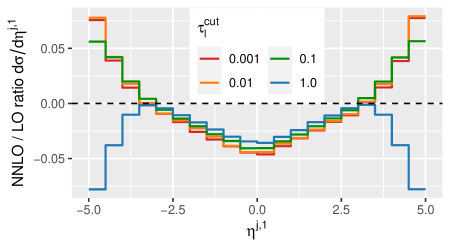
In fig. 3 we show the $\tau_{l}^{\text{cut}}$-dependence of the NNLO corrections for the leading jet pseudorapidity distribution as a fraction of the LO distribution. We use the anti-$k_{T}$ jet clustering with $R=0.5$. These are calculated for a stable top quark, that is ignoring the $b$-quark in the decay as a potential jet contributor. The absolute distribution (not shown here) therefore peaks around $\eta=\pm 2.5$, as its dominant contribution is from the forward jet on the light line.

Decreasing the slicing cutoff $\tau_{l}^{\text{cut}}$ exponentially by factors of 10, we see that the difference between $\tau_{l}^{\text{cut}}=0.001$ and $\tau_{l}^{\text{cut}}=0.01$ is negligible. Even for $\tau_{l}^{\text{cut}}=0.1$ the difference is small, especially in the central region. This demonstrates the successful cancellation of IR divergences through application of the slicing subtractions. Note that the corrections in the center are negative, while they are positive in the tails. In the absence of any cuts this leads to strong cancellations and a small NNLO correction to the inclusive cross section.

Figure 3: NNLO corrections from the light-line production vertex for the leading jet pseudorapidity distribution, relative to LO. The $\tau_{l}^{\text{cut}}$-dependence of the corrections is shown in the range $0.001$–$1.0$.

2.2 Top-quark-decay corrections

For the top-quark decay we make use of the factorization theorem described in refs. [69, 70, 71, 72, 73] for the observable

$$\tau_{d}=p_{X}^{2}/m_{t}^{2}\,,$$

where $p_{X}$ is the sum of all final-state parton momenta in the decay. The respective factorization theorem for corrections in decay and integrated over $\tau_{d}$ reads

$$\mathrm{d}\sigma_{ab}(\tau_{d}<\tau_{d}^{\text{cut}})=\mathrm{d}\sigma^{\text{Born}}f_{a}(x_{a},\mu)f_{b}(x_{b},\mu)\times\\ H(x,\mu)\int_{0}^{\tau_{d}^{\text{cut}}}\!\!\!\mathrm{d}\tau_{d}\int\!\mathrm{d}m^{2}\int\!\mathrm{d}k_{s}\,J(m^{2},\mu)\,S(k_{s},\mu)\,\delta\!\left(\tau_{d}-\frac{m^{2}+2E_{b}k_{s}}{m_{t}^{2}}\right)\,,$$ (6)

where $x=Q^{2}/m_{t}^{2}>0$, $E_{b}=(m_{t}^{2}-Q^{2})/(2m_{t})$ is the $b$-quark energy, and $Q^{2}=m_{W}^{2}$ for an on-shell $W$-boson. We also allow for the generation of the $W$-boson decay distributed according to a Breit-Wigner peak with $Q^{2}\neq m_{W}^{2}$.

We use the bare soft function $S_{\text{bare}}$ from ref. [74] and the bare jet function $J_{\text{bare}}$ from ref. [75]. We combined these with the bare hard function $H_{\text{bare}}$, which has been independently calculated in four different references [76, 77, 78, 79]. We perform all integral convolutions in Laplace-space and find successful cancellation of all IR poles between $J_{\text{bare}}$, $S_{\text{bare}}$ and $H_{\text{bare}}$. We furthermore checked that we can individually reproduce the renormalized results of the soft ($S$) and jet functions ($J$) as given in refs. [74, 75].

For the hard function we successfully checked the agreement between all four calculations using the Mathematica package HPL [81] for the evaluation of harmonic polylogarithms. We converted the hard function into an expression using only harmonic polylogarithms, so that our hard function implementation can be reused for the production part based on the automatic analytic continuation in the hplog Fortran code [82].

The matrix elements entering the above-cut calculation have been obtained by crossing from the virtual amplitudes used in the computation of $Wt$ production at NLO [52] and the real-radiation amplitudes employed in the four-flavor calculation of $t$-channel single-top production [83]. As for the corrections on the light-line, we cross-checked all amplitudes by a numerical comparison with Recola [68]. We then set up the NLO above-cut calculation using dipole subtractions. For the case of $q\to qg$ splitting with the massive top-quark spectator we have used the dipole expression from ref. [22], also presented in ref. [84]. The dipole expression for the $g\to gg$ splitting with the massive top spectator is taken from ref. [84].

Calculation of the top-quark decay width.

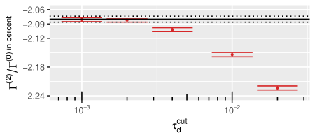
Our calculation can be used to compute the NNLO QCD corrections to the top-quark width. Such a calculation has previously been performed numerically in refs. [34, 35] (GLZ), as well as analytically as an expansion in $m_{W}^{2}/m_{t}^{2}$ [85, 86] (BCST). We write the perturbative corrections to the top-quark width as $\Gamma_{t}=\Gamma_{t}^{(0)}(1+\delta^{(1)}+\delta^{(2)})$, where the relative corrections of order $\alpha_{s}^{k}$ are written as $\delta^{(k)}\equiv\Gamma_{t}^{(k)}/\Gamma_{t}^{(0)}$ and $\Gamma_{t}^{(0)}$ is the LO decay width. In order to demonstrate the correctness of our calculation, in fig. 4 we show the $\tau_{d}^{\text{cut}}$-dependence of the NNLO corrections $\delta^{(2)}$ for the choice $\mu=m_{t}$ fig. 4. We observe a good convergence of the slicing procedure to the asymptotic value, finding no significant dependence around $\tau_{d}^{\text{cut}}=10^{-3}$.

A comparison of our calculation with previous results for the top-quark width is shown in table 1, demonstrating excellent agreement. The previous approximate results are confirmed at the 0.5% level for the second-order coefficient, corresponding to a difference of at most $0.01$% in the total width. The comparison is performed with $m_{t}=$172.5\text{\,}\mathrm{GeV}$$, but the relative size of the corrections is somewhat insensitive to the precise top-quark mass [34].

Figure 4: $\tau_{d}^{\text{cut}}$-dependence of the top-quark decay width NNLO corrections. Error-bars indicate numerical integration uncertainties. The solid line (with dashed band) indicates the fitted result (and uncertainties), which agrees with the result using $\tau_{d}^{\text{cut}}=10^{-3}$.

Table 1: Comparison between our calculation of the second-order correction to the top-quark width ($\delta^{(2)}$), as a percentage of the LO result of $1.4806\text{\,}\mathrm{GeV}$ ($m_{t}=$172.5\text{\,}\mathrm{GeV}$$), and previous computations of the same quantity from Gao et al. [34] ($\delta^{(2)}_{\text{GLZ}}{}$) and Blokland et al. [86] ($\delta^{(2)}_{\text{BCST}}{}$).

$\mu$	$\delta^{(2)}_{\text{BCST}}$	$\delta^{(2)}_{\text{GLZ}}$	$\delta^{(2)}$
$m_{t}$	$-2.07$	$-2.08$	$-2.08(1)$
$2m_{t}$	$-2.38$	$-2.39$	$-2.39(1)$
$m_{t}/2$	$-1.58$	$-1.58$	$-1.58(1)$

2.3 Top-quark-production corrections on the heavy line

For the heavy line production corrections we make use of the factorization theorem given in ref. [87] using the observable $\tau_{h}$ [54],

$$\tau_{h}=\frac{2p_{X}p_{b}}{m_{t}^{2}-q^{2}}\,,$$

where $p_{X}$ is the sum of the additionally radiated partons, $p_{b}$ is the $b$-quark beam momentum and $q^{2}$ is the momentum-squared of the $t-$channel $W$ boson ($q^{2}<0$).

The factorization theorem in $\tau_{h}$, integrated over $\tau_{h}$, reads

$$\mathrm{d}\sigma_{ab}(\tau_{h}<\tau_{h}^{\text{cut}})=\mathrm{d}\sigma^{\text{Born}}f_{a}(x_{a},\mu)\,\times\\ H(x+i0,\mu)\int_{0}^{\tau_{h}^{\text{cut}}}\!\!\!\mathrm{d}\tau_{h}\int\!\mathrm{d}t\int\!\mathrm{d}k_{s}\,B_{b}(x_{b},t,\mu)\,S(k_{s},\mu,\mu_{F})\,\delta\!\left(\tau_{h}-\frac{t+2k_{s}E_{b}}{m_{t}^{2}-q^{2}}\right)\,,$$ (7)

where $x=q^{2}/m_{t}^{2}$. $E_{b}=(m_{t}^{2}-q^{2})/(2m_{t})$ is the $b$-quark beam energy in the top-quark rest frame. We reuse the renormalized soft function $S$ from the top-quark decay [74]. This is possible when the soft function is defined in the top-quark rest frame as above and has been discussed in ref. [38]. We also reuse the beam functions $B_{b}$ [59, 54, 60] implemented through ref. [61]. The hard function $H$ is reused from the top-quark decay, but requires an analytic continuation. Since we implemented it in terms of harmonic polylogarithms, we can use the automatic analytic continuation of the hplog Fortran code [82]. We have verified that these analytically continued numerical results agree with an explicit analytic continuation in Mathematica using the HPL package [81]. Lastly, we have explicitly performed the integrals and distributional convolutions in Laplace space to obtain the assembled result in terms of $\log^{k}(\tau_{h})$ contributions. As for the other contributions, we analytically verified that the renormalization scale dependence vanishes to the corresponding order, or in other words, that all poles cancel between bare hard, soft and beam function. We also find full agreement between our $\tau_{h}$-subtraction results at NLO and a calculation using dipole subtractions [22]. The above-cut contributions are obtained by crossing from the matrix elements used in the decay corrections.

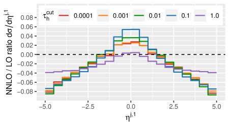
We show the NNLO corrections to the leading jet pseudorapidity distribution as a fraction of the LO result in fig. 5, as well as their dependence on $\tau_{h}^{\text{cut}}$. As for the light-line corrections, this distribution is calculated for a stable top quark, thereby ignoring the $b$-quark in the decay as a jet contributor. Comparing the results for the exponentially decreasing slicing cutoffs $\tau_{h}^{\text{cut}}$, we see that $\tau_{h}^{\text{cut}}=10^{-4}$ and $\tau_{h}^{\text{cut}}=10^{-3}$ differ only marginally within remaining numerical uncertainties. Even $\tau_{h}^{\text{cut}}=10^{-2}$ differs only in the most central bins. This demonstrates the successful cancellation of IR divergences. We conclude that $\tau_{h}^{\text{cut}}=0.001$ constitutes a sufficiently small cutoff for reliable results. Once more there are strong cancellations, that lead to a small correction to the inclusive cross section, since the corrections are small and positive in the central region and larger and negative towards the tails.

Figure 5: NNLO corrections from the heavy-line production vertex for the leading jet pseudorapidity distribution, relative to LO. The (automatically) fitted result coincides within numerical uncertainties with the $\tau_{h}^{\text{cut}}=10^{-3}$ result.

2.4 $\text{NLO}{}\otimes\text{NLO}{}$ interference contributions

Apart from two-loop vertex corrections, $\text{NLO}{}\otimes\text{NLO}{}$ contributions also arise at NNLO from production corrections times decay corrections (light $\otimes$ decay, heavy $\otimes$ decay) and light-line corrections times heavy-line corrections (light $\otimes$ heavy).

We implemented all of these contributions in a mixed scheme where one part of the NLO calculation is handled with dipole subtractions and the other half with NLO slicing subtractions, as described for the individual NNLO vertex corrections above. This makes the implementation within our existing infrastructure easier. Each of the three $\text{NLO}{}\otimes\text{NLO}{}$ calculations (light $\otimes$ decay, heavy $\otimes$ decay, light $\otimes$ heavy) consists of four contributions, categorized into real $\otimes$ real, (RR), real $\otimes$ virtual (RV), virtual $\otimes$ real (VR), and virtual $\otimes$ virtual (VV). The first part is always calculated with dipole subtractions and denotes the real emission contributions with dipole subtractions (real), and virtual loop corrections with integrated dipoles (virtual). The second part is calculated using the discussed factorization theorems and denotes the above-cut emission (real), and the below-cut loop contribution (virtual) from the integrated factorization theorem.

For each of the three $\text{NLO}{}\otimes\text{NLO}{}$ calculations we checked cancellation of poles for the dipole subtractions through the alpha parameter [50, 51, 22, 52, 53] for the RV+VV and RR+VR contributions separately. We furthermore checked for VV+VR and RV+RR separately that remaining $\tau^{\text{cut}}$ effects for our default choice of $\tau^{\text{cut}}=10^{-3}$ are negligible at the per-mille level and that the asymptotic approach is logarithmic as predicted by the factorization theorems. Therefore all four pieces of each $\text{NLO}{}\otimes\text{NLO}{}$ contribution are checked through a chain of tests.

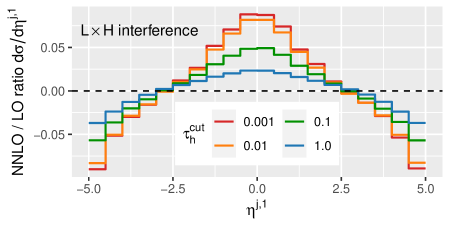
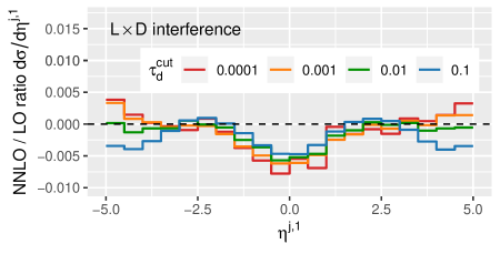
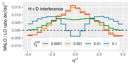
We show the differential $\tau^{\text{cut}}$-dependence for all three interference contributions in fig. 6 for the leading jet pseudorapidity distribution at $\sqrt{s}=$13\text{\,}\mathrm{TeV}$$ using anti-$k_{T}$ jet clustering with $R=0.5$. We indeed find that for $\tau^{\text{cut}}=10^{-3}$ residual power corrections are negligible at the single per-mille level.

While one might naively expect that the factorization between production and decay allows an implementation of NNLO interference corrections as the product of NLO corrections in production and decay, at the level of differential cross sections, this is not true. This property only holds fully inclusively, and serves as another check of the implementation, see eq. 2. For instance, the light $\otimes$ decay interference contribution ($\sigma_{L\times D}$) is equal to the light-line production NLO coefficient ($\sigma^{(1)}_{L}$) multiplied by the NLO width correction factor, $\Gamma^{(1)}/\Gamma^{(0)}=-0.0858$. As an example, at $\sqrt{s}=$13\text{\,}\mathrm{TeV}$$ we have,

$$\sigma_{L\times D}=$-154\pm 4.\text{\,}\mathrm{f}\mathrm{b}$\,,\qquad\sigma^{(1)}_{L}\times\frac{\Gamma^{(1)}}{\Gamma^{(0)}}=$-155\text{\,}\mathrm{f}\mathrm{b}$\,.$$ (8)

Furthermore, the heavy $\otimes$ decay interference ($\sigma_{H\times D}$) is also in excellent agreement,

$$\sigma_{H\times D}=$645\pm 4.\text{\,}\mathrm{f}\mathrm{b}$\,,\qquad\sigma^{(1)}_{H}\times\frac{\Gamma^{(1)}}{\Gamma^{(0)}}=$645\text{\,}\mathrm{f}\mathrm{b}$\,.$$ (9)

Figure 6: NNLO corrections to the leading jet pseudorapidity distribution, relative to LO, from light $\otimes$ heavy interference (upper panel), light $\otimes$ decay interference (center panel) and heavy $\otimes$ decay interference (lower panel).

3 Comparison with previous results

In section 2 we have presented extensive cross-checks of all parts of our calculation, ranging from the amplitudes, to analytical checks of the factorization theorems and their ingredients, to the numerical implementation. Thus, having confidently assessed the validity of our calculation, we now compare against the two previous calculations of this process. Like our calculation, these are also performed in the approximation of an on-shell top quark, but the previous results disagree on the size of the NNLO corrections.

3.1 Stable top quark

We first compare with the NNLO results computed by Brucherseifer, Caola and Melnikov (BCM) [36]. This calculation is performed in the stable-top-quark approximation and therefore does not include the decay of the top quark. To compare with their results we adopt $\sqrt{s}=$8\text{\,}\mathrm{TeV}$$, $m_{t}=$173.2\text{\,}\mathrm{GeV}$$, $m_{W}=$80.398\text{\,}\mathrm{GeV}$$, $G_{F}=$1.166\,39\text{\times}{10}^{-5}\text{\,}\mathrm{G}\mathrm{eV}^{-2}$$ and use the MSTW2008 PDF set [88] that corresponds to the order of the calculation. The resulting comparison between our calculation and the results of ref. [36] is shown in table 2, where we tabulate cross sections for four different minimum top-quark transverse momenta ($p_{T}$), including uncertainties due to scale variation.

While we find agreement at the per-mille level throughout NLO, we find discrepancies at the level of about $1$ to $1.5$ percent for the NNLO results. The calculational uncertainties for both our and the BCM results are about $0.1\text{\,}\mathrm{p}\mathrm{b}$, which is a relative uncertainty of two per-mille. A first re-calculation of single-top-quark production in refs. [37, 38] by Berger, Gao, Zhu (BGZ) has reported a similarly-sized difference to the BCM calculation. While these authors did not perform a direct comparison with the BCM results, we will demonstrate in section 3.2 a comparison with the results of BGZ that finds agreement at NNLO at a much greater level (within a few per-mille), even for fiducial and differential results.

Table 2: Comparison with fully inclusive top-quark production results from Brucherseifer, Caola, Melnikov in ref. [36]. Cross-sections in picobarns. Scale uncertainties in super- and subscript are from simultaneous variation of $\mu_{R}=\mu_{F}=m_{t}$ by a factor of two and one half, respectively.

$p_{T,\text{min}}^{\text{top}}$	$\sigma_{\text{LO}}^{\text{BCM}}$	$\sigma_{\text{LO}}\pm 0.01$	$\sigma_{\text{NLO}}^{\text{BCM}}$	$\sigma_{\text{NLO}}\pm 0.05$	$\sigma_{\text{NNLO}}^{\text{BCM}}$	$\sigma_{\text{NNLO}}\pm 0.1$
$0\text{\,}\mathrm{GeV}$	$53.8^{+3.0}_{-4.3}$	$53.79^{+3.03}_{-4.33}$	$55.1^{+1.6}_{-0.9}$	$55.15^{+1.63}_{-0.90}$	$54.2^{+0.5}_{-0.2}$	$\mathbf{53.5^{+0.65}_{-0.31}}$
$20\text{\,}\mathrm{GeV}$	$46.6^{+2.5}_{-3.7}$	$46.65^{+2.53}_{-3.66}$	$48.9^{+1.2}_{-0.5}$	$48.90^{+1.22}_{-0.54}$	$48.3^{+0.3}_{-0.02}$	$\mathbf{47.9^{+0.44}_{-0.16}}$
$40\text{\,}\mathrm{GeV}$	$33.4^{+1.7}_{-2.5}$	$33.41^{+1.67}_{-2.48}$	$36.5^{+0.6}_{-0.03}$	$36.55^{+0.59}_{-0.03}$	$36.5^{+0.1}_{+0.1}$	${36.5^{\mathbf{+0.15}}_{\mathbf{+0.04}}}$
$60\text{\,}\mathrm{GeV}$	$22.0^{+1.0}_{-1.5}$	$21.95^{+0.99}_{-1.52}$	$25.0^{+0.2}_{+0.3}$	$25.08^{+0.17}_{-0.27}$	$25.4^{-0.1}_{+0.2}$	$25.4^{\mathbf{+0.03}}_{\mathbf{+0.13}}$

Figure 7: $\tau^{\text{cut}}$ dependence of NNLO light, heavy, interference and summed contributions relative to the NLO part for the fully inclusive result in table 2. The dotted area represents the NNLO coefficient with an absolute uncertainty of $\pm$0.1\text{\,}\mathrm{p}\mathrm{b}$$ to obtain the result from Brucherseifer, Caola, Melnikov (BCM) [36].

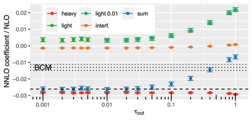
The numerical integration uncertainties and residual systematic uncertainty from our slicing cutoff $\tau^{\text{cut}}$ are at the per-mille level and small compared to the discrepancy we find. We first demonstrate this in the fully inclusive case ($p^{\text{top}}_{T,\text{min}}=0$) in fig. 7. We show the $\tau^{\text{cut}}$ dependence of the heavy-line contribution, light-line contribution, interference contribution and the sum, relative to the NLO part of the NNLO result. The black dotted area represents the (reconstructed) NNLO coefficient of BCM shown in table 2 with an absolute uncertainty of $\pm$0.1\text{\,}\mathrm{p}\mathrm{b}$$. Our numerical integration uncertainty is indicated by the error bars. All results have been obtained using the multi-$\tau^{\text{cut}}$ sampling in MCFM-9 with a minimum $\tau^{\text{cut}}$ of $10^{-3}$. Since the largest uncertainties are for the light-line contributions, the figure also shows a separate re-calculation of the light-line corrections with a nominal $\tau_{l}^{\text{cut}}$ value of $0.01$. These have a significantly smaller integration uncertainty but agree perfectly with results calculated with a nominal value of $\tau^{\text{cut}}=0.001$. Overall, with $\tau^{\text{cut}}=0.01$ we are already well within the asymptotic regime where results are precise at the per-mille level. The discrepancy with the BCM result is clearly visible and cannot be explained by calculational uncertainties or a difference in the NLO contribution.

Figure 8: $\tau^{\text{cut}}$ dependence of NNLO light, heavy, interference and summed contributions relative to the NLO part for the top-quark $p_{T}$ distribution as input to table 2. The black points with error bars represent the reconstructed results from Brucherseifer, Caola, Melnikov (BCM) [36], see table 2, with an absolute uncertainty of $\pm$0.1\text{\,}\mathrm{p}\mathrm{b}$$.

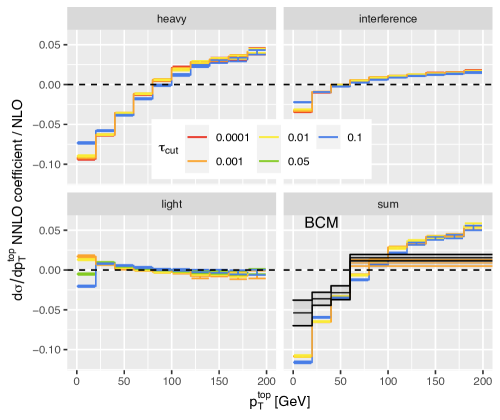
We next consider the top-quark $p_{T}$ distribution which, when integrated or summed over bins, reproduces the numbers in table 2 that require a minimum top-quark $p_{T}$. Also here we have to carefully inspect the $\tau^{\text{cut}}$ dependence, since it may manifest in a different way depending on the kinematics. For this we present top-quark $p_{T}$-differential results in fig. 8 for $\tau^{\text{cut}}$ values varying over three orders of magnitude. The results are presented normalized to the NLO part of the distribution, that is to the NLO cross section calculated with NNLO PDFs, to emphasize the relative size of the NNLO contributions. Just as in the fully inclusive case it is evident that with $\tau^{\text{cut}}=0.01$ the asymptotic regime is reached for all contributions, since it agrees well within our numerical uncertainties (small error bars) with the $\tau^{\text{cut}}=0.001$ result. For comparison with BCM we have reconstructed their corresponding results for the first three bins from table 2 and assume an absolute uncertainty of $\pm$0.1\text{\,}\mathrm{p}\mathrm{b}$$.

Our results show a definitive difference with the BCM results at both the differential and inclusive level. At the total level the discrepancy is about one percent. The discrepancy with the NNLO coefficient itself is 100%: For fully inclusive top-quark production our NNLO coefficient is $-$1.4\text{\,}\mathrm{p}\mathrm{b}$$, while the BCM coefficient is just $-$0.7\text{\,}\mathrm{p}\mathrm{b}$$. At the differential level the discrepancy is also large. For example for the top-quark $p_{T}$ distribution the difference in the first bin from $0\text{\,}\mathrm{GeV}20\text{\,}\mathrm{GeV}$ is six percent relative to NLO. For the last reconstructed bin for $p_{T}>$60\text{\,}\mathrm{GeV}$$ we agree within mutual uncertainties. We observe similarly-sized discrepancies for an anti-top quark, as detailed in table 3.

Table 3: Comparison with fully inclusive anti-top-quark production results from Brucherseifer, Caola, Melnikov in ref. [36]. Cross-sections in picobarns. Scale uncertainties in super- and subscript from simultaneous variation of $\mu_{R}=m_{t}$ and $\mu_{F}=m_{t}$ by a factor of two and one half, respectively.

$p_{T,\text{min}}^{\text{anti-top}}$	$\sigma_{\text{LO}}^{\text{BCM}}$	$\sigma_{\text{LO}}\pm 0.01$	$\sigma_{\text{NLO}}^{\text{BCM}}$	$\sigma_{\text{NLO}}\pm 0.05$	$\sigma_{\text{NNLO}}^{\text{BCM}}$	$\sigma_{\text{NNLO}}\pm 0.1$
$0\text{\,}\mathrm{GeV}$	$29.1^{+1.7}_{-2.4}$	$29.06^{+1.67}_{-2.38}$	$30.1^{+0.9}_{-0.5}$	$30.12^{+0.91}_{-0.48}$	$29.7^{+0.3}_{-0.1}$	$29.2^{+0.37}_{-0.19}$
$20\text{\,}\mathrm{GeV}$	$24.8^{+1.4}_{-2.0}$	$24.78^{+1.36}_{-1.97}$	$26.3^{+0.7}_{-0.3}$	$26.39^{+0.65}_{-0.26}$	$26.2^{-0.01}_{-0.1}$	$25.9^{+0.24}_{-0.10}$
$40\text{\,}\mathrm{GeV}$	$17.1^{+0.9}_{-1.3}$	$17.12^{+0.86}_{-1.28}$	$19.1^{+0.3}_{+0.1}$	$19.20^{+0.27}_{+0.05}$	$19.3^{-0.2}_{+0.1}$	$19.2^{\mathbf{+0.07}}_{\mathbf{+0.02}}$
$60\text{\,}\mathrm{GeV}$	$10.8^{+0.5}_{-0.7}$	$10.78^{+0.48}_{-0.75}$	$12.7^{+0.03}_{+0.2}$	$12.73^{+0.03}_{+0.20}$	$12.9^{-0.2}_{+0.2}$	$13.0^{\mathbf{-0.03}}_{\mathbf{+0.07}}$

3.2 Top quark production and decay

We now turn to a comparison with the re-calculation by Berger, Gao, Zhu (BGZ) [37, 38], who also include the top-quark decay and provide fully fiducial predictions and differential results with which to compare.

We first compare with inclusive cross sections (table 1 in ref. [38]), at $\sqrt{s}=7$ TeV and $\sqrt{s}=14$ TeV, for $t$ and $\bar{t}$. This comparison is performed with $m_{t}=$172.5\text{\,}\mathrm{GeV}$$, $m_{W}=$80.385\text{\,}\mathrm{GeV}$$, $G_{F}=$1.166\,379\text{\times}{10}^{-5}\text{\,}\mathrm{G}\mathrm{eV}^{-2}$$ and the CT14nnlo PDF set [89], irrespective of the order of the calculation that is considered. At NNLO we obtain all results with a nominal $\tau^{\text{cut}}=0.001$ but ensure through the multi-$\tau^{\text{cut}}$ sampling in MCFM-9 that the residual $\tau^{\text{cut}}$ dependence is small compared to our quoted combined integration and residual $\tau^{\text{cut}}$ uncertainty. The perturbative truncation uncertainties from scale variation are obtained by varying $\mu_{R}=\mu_{F}=m_{t}$ simultaneously by a factor of two and one half, respectively, so by a two-point variation. We do this to compare with the results in ref. [38], but note that with a six-point variation, where $\mu_{R}$ and $\mu_{F}$ are varied independently, the uncertainties increase at both NLO and NNLO. The results in table 4 show that, for both the central values and scale variations, the two calculations are in agreement at the level of less than three per-mille in the NNLO cross sections. Since our overall numerical and calculational precision is at the level of two to three per-mille, we consider this to be a excellent agreement, which is further supported by the following fiducial comparison.

Table 4: Comparison with fully inclusive production results from Berger, Gao, Zhu [38, 37]. Scale uncertainties in super- and subscript from simultaneous variation of $\mu_{R}=m_{t}$ and $\mu_{F}=m_{t}$ by a factor of two and one half, respectively.

		$\sigma_{\text{LO}}^{\text{BGZ}}$	$\sigma_{\text{LO}}$	$\sigma_{\text{NLO}}^{\text{BGZ}}$	$\sigma_{\text{NLO}}\pm 0.01$	$\sigma_{\text{NNLO}}^{\text{BGZ}}$	$\sigma_{\text{NNLO}}$
$7\text{\,}\mathrm{TeV}$	top	$44.55^{+5.3\%}_{-7.5\%}$	$44.55^{+5.3\%}_{-7.5\%}$	$43.14^{+2.9\%}_{-1.6\%}$	$43.15^{+2.9\%}_{-1.6\%}$	$42.05^{+1.2\%}_{-0.6\%}$	$41.99(4)^{+1.4\%}_{-0.7\%}$
	anti-top	$23.29^{+5.3\%}_{-7.6\%}$	$23.29^{+5.3\%}_{-7.6\%}$	$22.57^{+2.9\%}_{-1.5\%}$	$22.57^{+2.9\%}_{-1.5\%}$	$21.95^{+1.2\%}_{-0.7\%}$	$21.90(3)^{+1.4\%}_{-0.8\%}$
$14\text{\,}\mathrm{TeV}$	top	$164.4^{+8.4\%}_{-10\%}$	$164.41^{+8.4\%}_{-10.6\%}$	$157.8^{+3.0\%}_{-1.7\%}$	$157.78^{+2.9\%}_{-1.7\%}$	$153.3^{+1.1\%}_{-0.5\%}$	$153.2(2)^{+1.2\%}_{-0.6\%}$
	anti-top	$99.60^{+8.7\%}_{-11\%}$	$99.60^{+8.7\%}_{-10.9\%}$	$94.77^{+3.0\%}_{-1.6\%}$	$94.77^{+3.0\%}_{-1.7\%}$	$91.81^{+1.0\%}_{-0.5\%}$	$\enspace 91.5(1)^{+1.2\%}_{-0.7\%}$

We also successfully compared at the differential level for the fully inclusive process (stable top quark). For example, we show the leading jet pseudorapidity distribution in fig. 9 where agreement within numerical uncertainties can be seen. Although not illustrated explicitly here, the same holds true for the individual components of the calculation: heavy-line corrections, light-line corrections and light $\otimes$ heavy interference contributions.

Figure 9: Leading jet pseudorapidity distribution in stable top-quark production at LO, NLO and NNLO using NNLO CT14 PDFs. Our cross sections are compared with the results in ref. [38] (BGZ).

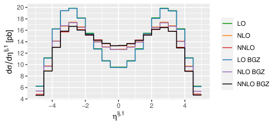
Comparison with fiducial results.

Table 5: Kinematical cuts at $\sqrt{s}=$13\text{\,}\mathrm{TeV}$$ for comparison with BGZ, ref. [38]. The top-quark mass is $173.3\text{\,}\mathrm{GeV}$.

Lepton cuts	$p_{T}^{l}>$30\text{\,}\mathrm{GeV}$,\lvert\eta^{l}\rvert<2.4$
anti-$k_{T}$ jet clustering	$p_{T}^{j}>$40\text{\,}\mathrm{GeV}$,R=0.5,\lvert\eta_{j}\rvert<5$
jet requirements	exactly two jets; with least one $b$ jet and $p_{T}$-leading $b$ jet $\lvert\eta\rvert<2.4$.

We now compare with the fiducial results in ref. [38] (BGZ), where we adopt $m_{t}=$173.3\text{\,}\mathrm{GeV}$$ and the kinematical cuts are summarized in table 5.

The results of this comparison are presented in table 6. Through NNLO we find agreement for all contributions within mutual uncertainties, where we assume an uncertainty of one in the final digit of the BGZ results. In addition to this we have performed a check of the individual contributions to the top-quark production number of $-0.24\text{\,}\mathrm{p}\mathrm{b}$ in table 6 from corrections to the light-line, heavy-line and heavy-light interference. For the light-line contribution we find $-100\pm 2.\text{\,}\mathrm{f}\mathrm{b}$, in agreement with $-100\text{\,}\mathrm{f}\mathrm{b}$ (BGZ), and the interference contribution is identical, $135\pm 1.\text{\,}\mathrm{f}\mathrm{b}$ compared to $135\text{\,}\mathrm{f}\mathrm{b}$ (BGZ). However, the heavy-line production contribution differs slightly: we find $-260\pm 2.\text{\,}\mathrm{f}\mathrm{b}$, to be compared with $-273\text{\,}\mathrm{f}\mathrm{b}$ (BGZ). While this tension is relatively large on the NNLO heavy-line production coefficient itself, it is only a per-mille level effect on the full NNLO result and does not affect the overall level of agreement. Subsequent communication regarding this comparison revealed a small error in the earlier published calculation that has now been identified and this small discrepancy is now understood.

Table 6: Comparison with fiducial results in ref. [38, 37]. Cross sections are given in pb.

		$\sigma_{\text{LO}}^{\text{BGZ}}$	$\sigma_{\text{LO}}$	$\sigma_{\text{NLO}}^{\text{BGZ}}$	$\sigma_{\text{NLO}}$	$\sigma_{\text{NNLO}}^{\text{BGZ}}$	$\sigma_{\text{NNLO}}$
top	total	$4.067$	$4.07$	$2.95$	$2.94$	$2.70$	$2.70$
	production			$-0.79$	$-0.792(1)$	$-0.24$	$-0.225(3)$
	decay			$-0.33$	$-0.338(1)$	$-0.13$	$-0.126(1)$
	prod. $\times$ decay					$+0.12$	$+0.117(1)$
anti-top	total	$2.45$	$2.45$	$1.78$	$1.78$	$1.62$	$1.62$
	production			$-0.46$	$-0.460(1)$	$-0.15$	$-0.153(3)$
	decay			$-0.21$	$-0.210(1)$	$-0.08$	$-0.078(1)$
	prod. $\times$ decay					$+0.07$	$+0.072(2)$

In contrast to our fiducial results that we present in the next section, the authors of ref. [38] use NNLO PDFs throughout their study, and so also for NLO predictions. They furthermore estimate scale uncertainties using a two-point variation ($\mu_{R}=\mu_{F}=k\cdot m_{t},k=\nicefrac{{1}}{{2}},2$) and a quadrature procedure from production and decay contributions. Their scale uncertainties of ${}^{+4.1\%}_{-2.2\%}$ and ${}^{+1.2\%}_{-0.7\%}$ at NLO and NNLO, respectively, increase to ${}^{{+6.1\%}}_{{-4.0\%}}$ at NLO and ${}^{+2.3\%}_{-2.1\%}$ at NNLO when a standard six-point scale variation (defined later, in section 4) is used. These uncertainties are mostly driven by the renormalization scale variation.

The use of NNLO PDFs leads to NNLO corrections of about $-9\%$ relative to NLO, see table 6, and the two-point quadrature scale-variation procedure leads to relatively small uncertainties, such that one observes a large gap between the NLO and NNLO predictions. This large difference shrinks to about $-5\%$ when NLO PDFs are used consistently at NLO, and one finds agreement within scale uncertainties. The consistent use of PDFs is crucial for the $t$-channel single-top-quark process. In fact, the authors speculate about the smallness of the total inclusive NNLO corrections due to DIS data used for PDF fits and that the $t$-channel process mimics double deep inelastic scattering. To fully exploit this property, it is essential that the order of the PDFs is consistent with the hard scattering cross section order. This property transfers also to the fiducial region to some extent, but depends on the inclusiveness of the cuts. The double DIS aspect can be maximally exploited in the factorized vertex-correction approach that we work with, namely by using DDIS scales, where one then expects a maximum of perturbative stability of predictions. This point will be discussed further in the following section.

4 Results

In this section we examine both the fully inclusive cross sections and the differential distributions relevant to experimental analyses. Stability of inclusive cross sections between perturbative orders is a signature of $t$-channel single-top-quark production, particularly when calculated with the DDIS scales, as it is effectively undoing the DIS fits to the PDFs [90]. The differential distributions are used for a variety of experimental signatures as both a signal process and as a background to any process that includes $W+$jets, e.g. $WH$ or supersymmetry. We describe below large differences between NLO and NNLO in key distributions that are used to distinguish signal from background.

We begin by presenting fully inclusive results for $7\text{\,}\mathrm{TeV}$ and $14\text{\,}\mathrm{TeV}$ proton-proton collisions (LHC) and for $1.96\text{\,}\mathrm{TeV}$ proton-antiproton collisions (Tevatron) in table 7. We show results using fixed scales $\mu_{R}=\mu_{F}=m_{t}$ for comparison with other results, and using the DDIS scales. Scale uncertainties are obtained using a six-point scale variation by evaluating the cross section for the scale choices $(k_{F}\cdot\mu_{F};k_{R}\cdot\mu_{R})$, where $\mu_{F}$ and $\mu_{R}$ are the central scales and

$$(k_{F};k_{R})\in\{(2,2),(0.5,0.5),(2,1),(1,1),(0.5,1),(1,2),(1,0.5)\}\,.$$

Subsequently maximum and minimum values are taken as the envelope. Our default PDF set in this section is CT14 [89] and we use it at a consistent order together with the partonic cross section order. That is, we use NLO PDFs for our NLO prediction and NNLO PDFs for our NNLO prediction. PDF uncertainties are given by evaluating the 56 eigenvector members (using DDIS scales).

Table 7: Fully inclusive results in pb for $pp$ at $7\text{\,}\mathrm{TeV}$ and $14\text{\,}\mathrm{TeV}$ (LHC), as well as $p\bar{p}$ at $1.96\text{\,}\mathrm{TeV}$ (Tevatron) with scales $\mu_{R}=\mu_{F}=m_{t}$ and DDIS scales and using CT14 PDFs. Uncertainties next to the cross section in super- and subscript are from a six-point scale variation, while PDF uncertainties are below.

	$7\text{\,}\mathrm{TeV}$ $pp$		$14\text{\,}\mathrm{TeV}$ $pp$		$1.96\text{\,}\mathrm{TeV}$ $\bar{p}p$
	top	anti-top	top	anti-top	$t+\bar{t}$
$\sigma_{\text{LO}}^{\mu=m_{t}}$	$37.1^{+7.1\%}_{-9.5\%}$	$19.1^{+7.3\%}_{-9.7\%}$	$134.6^{+10.0\%}_{-12.1\%}$	$78.9^{+10.4\%}_{-12.6\%}$	$2.09^{+0.8\%}_{-3.1\%}$
$\sigma_{\text{LO}}^{\text{DDIS}}{}$	$39.5^{+6.4\%}_{-8.6\%}$	$19.9^{+7.0\%}_{-9.3\%}$	$140.9^{+9.4\%}_{-11.4\%}$	$80.7^{+10.2\%}_{-12.3\%}$	$2.31^{-0.3\%}_{-1.8\%}$
$\sigma_{\text{NLO}}^{\mu=m_{t}}$	$41.4^{+3.0\%}_{-2.0\%}$	$21.5^{+3.1\%}_{-2.0\%}$	$154.3^{+3.1\%}_{-2.3\%}$	$91.4^{+3.1\%}_{-2.2\%}$	$1.96^{+3.1\%}_{-2.3\%}$
$\sigma_{\text{NLO}}^{\text{DDIS}}{}$	$41.8^{+3.3\%}_{-2.0\%}$	$21.5^{+3.4\%}_{-1.6\%}$	$154.4^{+3.7\%}_{-1.4\%}$	$91.2^{+3.1\%}_{-1.8\%}$	$2.00^{+3.6\%}_{-3.4\%}$
	PDF$\,{}^{+1.7\%}_{-1.4\%}$	PDF$\,{}^{+2.2\%}_{-1.5\%}$	PDF$\,{}^{+1.7\%}_{-1.1\%}$	PDF$\,{}^{+1.9\%}_{-0.9\%}$	PDF$\,{}^{+4.3\%}_{-5.3\%}$
$\sigma_{\text{NNLO}}^{\mu=m_{t}}$	$41.9^{+1.2\%}_{-0.7\%}$	$21.9^{+1.2\%}_{-0.7\%}$	$153.3(2)^{+1.0\%}_{-0.6\%}$	$91.5(2)^{+1.1\%}_{-0.9\%}$	$2.08^{+2.0\%}_{-1.3\%}$
$\sigma_{\text{NNLO}}^{\text{DDIS}}{}$	$41.9^{+1.3\%}_{-0.8\%}$	$21.8^{+1.3\%}_{-0.7\%}$	$153.4(2)^{+1.1\%}_{-0.7\%}$	$91.2(2)^{+1.1\%}_{-0.9\%}$	$2.07^{+1.7\%}_{-1.1\%}$
	PDF$\,{}^{+1.3\%}_{-1.1\%}$	PDF$\,{}^{+1.4\%}_{-1.3\%}$	PDF$\,{}^{+1.2\%}_{-1.0\%}$	PDF$\,{}^{+1.0\%}_{-1.0\%}$	PDF$\,{}^{+3.7\%}_{-5.0\%}$

While there are noticeable differences in the inclusive cross section between DDIS scales and $\mu=m_{t}$ at LO, the differences are within scale uncertainties at the LHC. At the Tevatron the large difference is due to cancellations between corrections on the light-quark line and the bottom-quark line, and the LO scale uncertainties grow to $\pm 7\%$ when varied independently [19]. Overall we see that the NNLO corrections are almost zero and that NLO and NNLO results overlap well within the small scale uncertainties of $\sim 1\%$. PDF uncertainties are at a similar level, but larger for the Tevatron.

For the Tevatron it is noteworthy that when using the DDIS scales and CT14 PDFs the cross section varies by 10–15% between LO and NLO [90]. This large difference, which should vanish for pure DIS data and fully correlated fits, shrinks to a few percent between NLO and NNLO. Whether this is an artifact of these particular PDF fits or is a sign of a deeper problem with the way PDFs are parameterized is material for a dedicated study [91].

4.1 Fiducial and differential cross sections

The key to understanding signals and backgrounds in $t$-channel single-top-quark analyses are the $W$+$n$-jet exclusive cross sections. The $2$-jet cross section with exactly one $b$-quark tag is enriched with the $t$-channel signal, while the $3$-jet cross section with one or two $b$-quark tags is dominated by background processes like $t\bar{t}$. It is essential that precise predictions are available for both the signal region of $t$-channel single-top-quark production, but also for the background region, which subsequently constraints the $t\bar{t}$ contribution in final fits. In practice, the final extraction is done using a multivariate analysis with various discriminator observables, see e.g. ref. [92].

Our initial acceptance cuts are inclusive and defined in table 8. We require at least one $b$-tagged jet and one non-$b$-tagged (light) jet in order to study the effect of the NNLO corrections on jet counting. In the results presented below we reconstruct the top-quark momentum by adding the exact $W$-boson momentum and the momentum of the $b$-jet with the largest $p_{T}$. We are particularly interested in reconstructed $t$+$n$-jet observables. In the following $j_{b}$ denotes a $b$-tagged jet and $j_{l}$ a light-quark jet (not $b$ tagged), while $j$ without any subscripts labels any kind of jet.

Table 8: Our fiducial cuts at $\sqrt{s}=$13\text{\,}\mathrm{TeV}$$.

Lepton cuts	$p_{T}^{l}>$25\text{\,}\mathrm{GeV}$,\lvert\eta^{l}\rvert<2.5$
anti-$k_{T}$ jet clustering	$p_{T}^{j}>$30\text{\,}\mathrm{GeV}$,R=0.4,\lvert\eta_{j}\rvert<4.5$
jet requirements	at least one non-$b$ (light) jet and at least one $b$ jet

For our set of cuts we find that, when PDFs are evaluated at the same order as the matrix element correction, the total fiducial NNLO prediction $\sigma^{\text{NNLO}}{}=$5.75\text{\,}\mathrm{p}\mathrm{b}$$ agrees with the NLO prediction $\sigma^{\text{NLO}}{}=$5.65\text{\,}\mathrm{p}\mathrm{b}$$ within less than two percent (see table 9). The stability across orders is due to a consistent use of PDF orders. We also see a significant reduction in the scale uncertainty of the individual exclusive $tj$ and $tjj$ channels from $\sim 10$–$15\%$ at NLO to $\sim 5$–$8$% at NNLO. The prediction for $tjjj$ is a LO prediction with correspondingly larger uncertainties. The $tjjj$ exclusive channel uncertainty dominates the semi-inclusive $tj_{l}$ fiducial uncertainty at NNLO, which is therefore not much smaller than the NLO uncertainty.

However, while the semi-inclusive cross section is stable with small uncertainties, there is a large 20% shift of events from the $t+2$-jet bin to the $t+3$-jet bin (along with a small reduction of the cross section in the $t+1$-jet signal bin) when moving from NLO to NNLO. This is very significant because the $t+2$-jet bin is precisely the bin on which the cut is made to separate signal from background. In practice, the experimental data in each of the jet bins is normalized to the relative fraction predicted by theory, and the absolute cross section is floated to match the inclusive data. This means that the while the signal prediction in $tj$ goes down by 5% at NNLO, too many events are being cut if the NLO normalization is used for the $tjj$ bin. Hence, the net signal predicted by NNLO will increase compared to NLO, and the $tjj$ background to other physics processes is smaller than expected by NLO.

Table 9: Cross sections for the production of a top quark ($W$ plus $p_{T}$-leading $b$-jet) and additional jets using DDIS scales, in pb. The cross sections are given in the fiducial region as in table 8, but apart from the inclusive $tj_{l}$ row the jet requirements are adjusted accordingly. $j_{b}$ denotes a $b$-tagged jet and $j_{l}$ a light-quark jet (not $b$ tagged). Contributions with more than one additional $b$-tagged jet are negligible and omitted. Uncertainties from a six point scale variation are given in super- and subscript. Percentages in parenthesis give the fraction with respect to the individual inclusive jet category. Numbers in bold font in each column add up to the $tj_{l}$ inclusive result within numerical uncertainties.

	LO	NLO	NNLO
$tj_{l}$ inclusive	$5.51^{+9.1\%}_{-11\%}$	${5.65}^{+3.8\%}_{-3.1\%}$	${5.75}^{+3.3\%}_{-2.7\%}$
$tj$	$5.51^{+9.1\%}_{-11\%}$	$3.77^{+10.0\%}_{-9.8\%}$ (100%)	$3.55^{+7.1\%}_{-5.9\%}$ (100%)
$tj_{l}$	$5.51^{+9.1\%}_{-11\%}$	$\mathbf{3.24}^{+13.6\%}_{-13.2\%}$ (86%)	$\mathbf{3.08}^{+8.2\%}_{-6.5\%}$ (87%)
$tj_{b}$	—	$0.53^{+14.9\%}_{-12.2\%}$ (14%)	$0.47^{+2.5\%}_{-5.3\%}$ (13%)
$tjj$	—	$\mathbf{2.42}^{+10.4\%}_{-9.2\%}$ (100%)	$\mathbf{1.90}^{+4.3\%}_{-7.6\%}$ (100%)
$tj_{l}j_{l}$	—	$0.93^{+10.6\%}_{-8.7\%}$ (38%)	$0.75^{+4.2\%}_{-5.9\%}$ (40%)
$tj_{b}j_{l}$	—	$1.49^{+15.3\%}_{-12.5\%}$ (62%)	$1.15^{+4.5\%}_{-9.9\%}$ (60%)
$tjjj$	—	—	$\mathbf{0.77}^{+27.3\%}_{-20.0\%}$ (100%)
$tj_{l}j_{l}j_{l}$	—	—	$0.13^{+20.0\%}_{-15.1\%}$ (17%)
$tj_{b}j_{l}j_{l}$	—	—	$0.64^{+30.0\%}_{-21.4\%}$ (83%)

Differential cross sections.

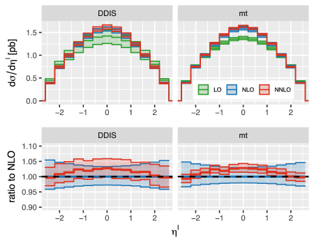
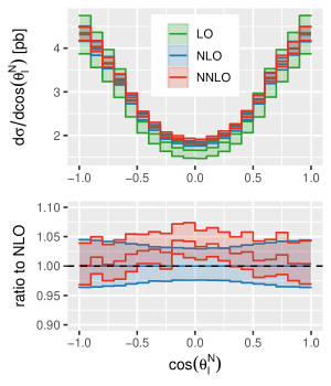
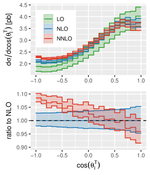
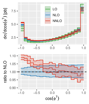
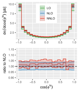
We now move on to discuss differential distributions. For all the following plots we show absolute distributions with scale uncertainties in the upper panel, while in the lower panel we show the ratios $\text{NNLO}{}/\text{NLO}{}$ and $\text{NLO}{}/\text{NLO}{}$ to study perturbative stability across orders. For the ratios we show the scale uncertainties from variation in the numerator only. Perturbative stability across orders can therefore be judged by examining the extent to which the uncertainty bands overlap.

We begin our discussion with the charged lepton pseudorapidity distribution shown in fig. 10 at LO, NLO and NNLO. This distribution is mostly kinematically driven and, as expected, the NNLO corrections are consistent with zero to within a few percent fully differentially. The differences in the central prediction between DDIS scales and fixed scale $m_{t}$ are small at NNLO, but we observe noticeably larger scale uncertainties using the DDIS scales, allowing for a robust overlap of predictions from LO through NNLO. The relatively large scale uncertainties at NNLO, compared to NLO, were already visible in the $tj_{l}$ inclusive cross section in table 9 and are an artifact of the specific set of rather inclusive cuts. Compare this, for example, with the fully inclusive uncertainties in table 7, which are much smaller at the level of $1\%$ and the large uncertainty decrease in the individual jet cross sections in table 9. Overall, the large scale uncertainties are also consistent with the observation that the NNLO effects are almost as large as the NLO effects.

For all other distributions we find similar central results between DDIS and $m_{t}$ scales. Since DDIS scales are the most consistent with the DIS nature of the $t$-channel process we only show the DDIS results with their more robustly estimated scale uncertainties.

Figure 10: Pseudorapidity distribution of the charged lepton with DDIS scales (left) and fixed scale $m_{t}$ (right).

Figure 11: Top-quark transverse momentum distribution (left) and rapidity distribution (right).

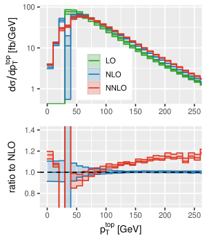
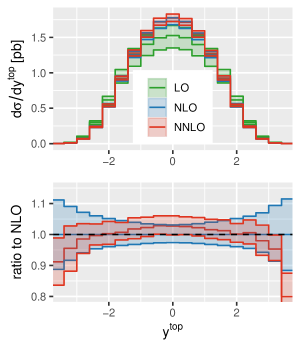
Other standard observables to consider are the top-quark transverse momentum and rapidity. We show these distributions in fig. 11. The NNLO rapidity corrections are small and consistent with zero within scale uncertainties. The NNLO transverse momentum corrections are, on the other hand, sizable and correct NLO results by up to +15% at $200\text{\,}\mathrm{GeV}250\text{\,}\mathrm{GeV}$. Kinematically, the top quark $p_{T}$ is driven by recoil from additional jets beginning at an NLO calculation. Therefore, one expects to see large effects at NNLO, which we observe here and which are outside scale uncertainty bands. The kinematic jet recoil threshold around $30\text{\,}\mathrm{GeV}$ is also significantly stabilized at NNLO by the additional radiation. This threshold region had to be addressed previously by a parton shower or partial resummation.

$t$-channel signal and background.

In addition to jet counting, the most important discriminatory observable for the signal is the light-quark jet pseudorapidity, which in $t$-channel production has its distinctive peak in the forward direction. In fig. 12 we present the ($p_{T}$) leading light-jet transverse momentum and pseudorapidity distributions. NNLO corrections drive the transverse momentum slightly harder in the tail but have little effect in the peak region. The shape of the pseudorapidity distribution changes noticeably, with negative corrections of $10\%$ in the very forward region and positive corrections of $20\%$ in the central region, leaving the peak region with corrections of just a few percent.

The leading $b$-jet distributions shown in fig. 13 are relevant for the top-quark reconstruction and enter directly in our previously shown top-quark distributions. For the transverse momentum we observe zero corrections in the peak region but positive corrections of $15\%$ at large $p_{T}$ driven by additional recoil available at NNLO. The pseudorapidity distribution receives only positive corrections of $2-3\%$ in the relevant peak region.

Another important discriminatory observable is the angle between the lepton and the leading light-quark jet in the top-quark rest frame, which we discuss later.

Figure 12: $p_{T}$-leading light jet transverse momentum distribution (left) and pseudorapidity distribution (right).

Figure 13: $p_{T}$-leading $b$-tagged jet transverse momentum distribution (left) and pseudorapidity distribution (right).

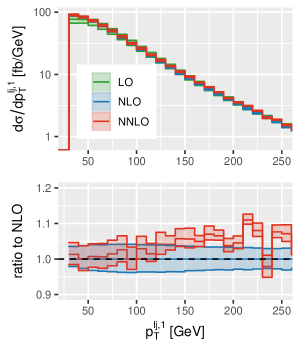
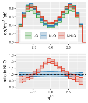
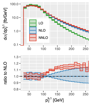
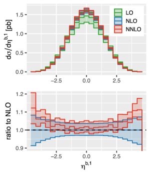
Moving to the relevant distributions for a proper background estimation, we show the subleading light-quark jet and subleading $b$-tagged jet transverse momentum and pseudorapidity distributions in figs. 14 and 15, respectively. Since these distributions enter for the first time at NLO in our five-flavor scheme calculation, the $\alpha_{s}$ corrections at NNLO are large and significant. And while these distributions could be obtained from an NLO event generator with a Born process of single-top-quark production plus an additional jet ($W$+3-jet production), the calculation within our NNLO framework allows for a correct normalization of these background contributions to the signal contribution.

Figure 14: $p_{T}$-subleading light jet transverse momentum distribution (left) and pseudorapidity distribution (right).

Figure 15: $p_{T}$-subleading $b$-tagged jet transverse momentum distribution (left) and pseudorapidity distribution (right).

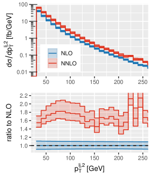
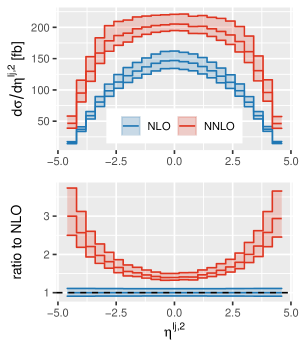
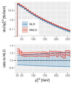
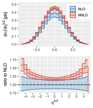
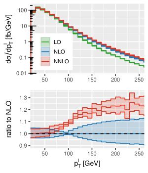
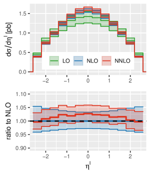
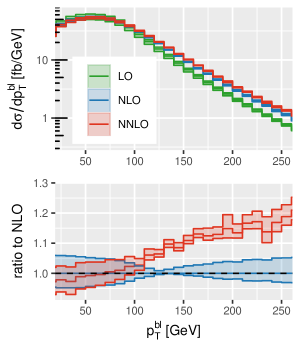
In appendix A we present additional distributions for the lepton transverse momentum, see fig. 17, and the $b$-quark-lepton system invariant mass and transverse momentum, see fig. 18.

Angular observables in the top-quark rest frame.

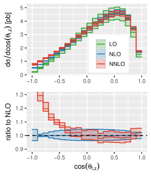
In addition to assessing the impact of higher order corrections on the usual kinematical distributions such as invariant masses, transverse momenta and rapidities, it is important to also consider their effect on angular correlations. The angle between the leading non-$b$ jet and the lepton from the top-quark decay in the top-quark rest frame [21] exhibits a strong correlation [93, 94] and is one of the key observables used to identify the $t$-channel process. Our NNLO results for this observable $\cos(\theta_{l,z})$ are shown in fig. 16 and we find that NNLO corrections are consistent with zero for the bulk region. At large angles ($\cos\theta_{l,z}\sim-1$) the additional radiation at NNLO becomes important and the corrections are significant, as expected.

Figure 16: Angular distribution for $\cos\theta_{l,z}$.

.

Several other angular distributions measured in the top-quark or $W$-boson rest frame are expected to be modified by non-standard model physics effects [95, 96]. Such angles are constructed to be sensitive to new physics in the production and decay stages of the top quark, respectively. We present NNLO results for two such sets of angles in fig. 18 and find that NNLO corrections are mostly consistent with zero in the bulk regions within a few percent of scale uncertainties. For the study of anomalous couplings and SMEFT contributions this perturbative stability at NNLO is important, since such analyses are performed at NLO. In fact, the inclusion of off-shell effects at NLO has previously been found to be equally or more important for some angular distributions [33].

5 Conclusions

We have presented a calculation of $2\to 4$ (five-flavor scheme) $t$-channel single-top-quark production and decay at NNLO. Due to the special importance of the top quark in the Standard Model, and the availability of large, high-quality data sets from the LHC experiments, predictions at this level of sophistication are mandatory for future analyses. Moreover, such calculations should be cross-checked carefully and made available publicly in order to facilitate any such studies.

Our calculation is performed in the on-shell and vertex-function approximation that allows for a factorization into NNLO corrections in production on the light-quark line, heavy-quark line and corrections in decay. We include all NNLO vertex corrections through three NNLO calculations but also the $\text{NLO}{}\otimes\text{NLO}{}$ interference contributions between light line and heavy line, as well as production and decay at the amplitude level, thereby preserving all spin correlations between production and decay. We performed extensive checks of all components of our calculation, and at all stages of the assembly. This includes analytical checks of all ingredients entering the factorization theorems used for our NNLO subtractions, comparisons of individual amplitudes with the numerical one-loop library Recola, and verification of our numerical implementations of dipole subtractions and slicing subtractions at the per-mille level.

With the results of our calculation we have been able to scrutinize the results of the stable top-quark calculation [36] and the results with decay in refs. [37, 38]. We find full agreement with the latter calculation at the per-mille level, but in the former case find differences of 100% on the total NNLO coefficient and up to six percent in the full NNLO top-quark $p_{T}$ distribution. Our calculation therefore resolves this discrepancy and, furthermore, validates the first implementation of differential NNLO corrections in the decay [34, 37, 38].

A special focus of our implementation is to keep full flexibility for dynamic factorization and renormalization scales in all parts of the calculation. One is then able to exploit that single-top-quark production is like double deep inelastic scattering (DDIS) in the approximation that we use, and set the scales as they are used in the fitting of PDFs from light-quark and heavy-quark DIS data. While the effect of using DDIS scales compared to using a fixed scale $m_{t}$ seems small at NLO and NNLO for the PDF set considered here, it can serve as a consistency check and constraint of PDFs that we intend to pursue in a subsequent study.

We presented total cross sections at the fully inclusive level including scale uncertainties and PDF uncertainties for the $7\text{\,}\mathrm{TeV}$ and $14\text{\,}\mathrm{TeV}$ LHC and for proton-antiproton collisions at the Tevatron for both a fixed central scale as well as DDIS scales. We studied fiducial cross sections at the total and the differential level in detail, presenting standard kinematical distributions used for single-top-quark analyses. We estimate scale uncertainties using a standard six-point variation and DDIS central scales. With this prescription we find that uncertainties are about a factor of two larger than in the previous calculation [38], which employed a different prescription, but our choice better represents the differential variation order-by-order.

Overall we find that NNLO corrections are crucial for a precision identification of the $t$-channel process, whose primary discriminatory observable is the leading light-quark jet pseudorapidity. This observable receives shape corrections of up to 20% at NNLO. Higher-order effects are also important for the background categories of $W$+3-jet production where corrections are 50–100%. We also showed NNLO predictions for certain sets of angles defined in the top-quark rest frame that are sensitive to new physics in the production and decay vertices. We find that NNLO corrections for these angles are small and that therefore these angles are kinematically robust and can be taken into account at NLO at the current level of precision for the search for new physics.

In the future it could be interesting to investigate if the use of DDIS scales can provide a useful constraint on PDFs. The general relevance of $t$-channel single-top-quark production for PDF fits has been studied before in ref. [97]. To further improve the accuracy of our predictions, NLO off-shell effects implemented in MCFM [33] could be incorporated with a reweighting procedure. Additionally, one could furthermore work towards the inclusion of the $1/N_{c}^{2}$ color-suppressed effects from two-loop box diagrams, which should be feasible with modern loop-calculation techniques.

Our calculation will be made publicly available in an upcoming version of MCFM to be useful directly for the LHC precision physics program.

Acknowledgments

We would like to thank Jun Gao for providing information regarding the calculation presented in ref. [38]: for supplying us with more detailed cross section numbers for comparison, that allowed for the exhaustive cross-check detailed in table 6 and the surrounding discussion, as well as for clarifying the details of the scale variation procedure. We furthermore thank Jean-Nicolas Lang for providing us with Recola 4-flavor and 5-flavor scheme model files.

This document was prepared using the resources of the Fermi National Accelerator Laboratory (Fermilab), a U.S. Department of Energy, Office of Science, HEP User Facility. Fermilab is managed by Fermi Research Alliance, LLC (FRA), acting under Contract No. DE-AC02-07CH11359. Tobias Neumann is supported by the United States Department of Energy under Grant Contract DE-SC0012704. The numerical calculations reported in this paper were performed using the Wilson High-Performance Computing Facility at Fermilab.

Appendix A Additional fiducial distributions

In this Appendix we provide supplementary figures for select kinematic distributions and angular correlations using the fiducial cuts of table 8 in section 4.1.

In fig. 17 we present the NNLO transverse momentum and pseudorapidity distributions for the lepton from the top-quark decay. The NNLO corrections in the pseudorapidity distribution are at the level of a few percent but still consistent with zero within scale uncertainties, as may be expected from our total fiducial cross section in table 9. The transverse momentum distribution on the other hand receives sizable corrections in the tail, but is perturbatively stable in the peak region. The corrections in the tail are large because the transverse recoil is driven by the subleading jet in the decay, entering for the first time at NLO.

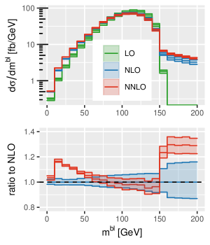
Combinations of the leading $b$-jet and lepton system are relevant for the top-quark mass measurement in $t$-channel production [98, 3] since they allow one to circumvent the neutrino reconstruction. We show the $bl$ transverse momentum and invariant mass distribution in fig. 18 and find that while NNLO corrections are small in the peak regions, they are important otherwise. The large perturbative corrections to the transverse momentum distribution follow directly from the stiffening of the lepton transverse momentum at NNLO that is included in this variable.

Figure 17: Positron transverse momentum distribution (left) and pseudorapidity distribution (right).

Figure 18: Leading $b$-tagged jet plus lepton transverse momentum distribution (left) and invariant mass distribution (right).

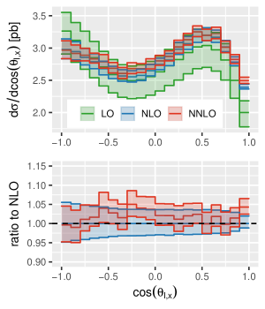
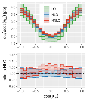
We also present NNLO results for two sets of angular observables that are sensitive to modifications from new physics in the top-quark production and decay stages, respectively. To describe the first set of angles we introduce a coordinate system that uses the direction of the leading light-quark jet $\vec{s}_{t}$ in the top-quark rest frame to define the $z$-axis, $\hat{z}$. The leading light-quark jet is identified at LO with the quark radiated on the light-quark line and is referred to as the spectator quark in the literature. This identification is only well-defined at LO, of course. The direction orthogonal to the plane made by the spectator quark and the initial-state light-quark defines the $y$-axis, $\hat{y}$. The initial-state light-quark direction, ($\vec{p}_{q}$), is chosen by selecting the beam direction whose rapidity has the same sign as that of the spectator jet. Finally, the coordinate system is completed by defining $\hat{x}$ such that the system is right-handed [95]. Thus we have,

$$\hat{z}=\frac{\vec{s}_{t}}{|\vec{s}_{t}|},\quad\hat{y}=\frac{\vec{s}_{t}\times\vec{p}_{q}}{|\vec{s}_{t}\times\vec{p}_{q}|},\quad\hat{x}=\hat{y}\times\hat{z}\,.$$ (10)

The (cosines of the) angles of the lepton with respect to these axes are referred to as $\cos\theta_{l,x},\cos\theta_{l,y},\cos\theta_{l,z}$. Generically, these angles are sensitive to operators that modify the production of the top quark.

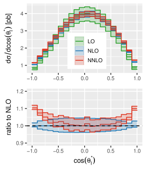
The second system uses as its first axis the direction of the $W$-boson in the top-quark rest frame, $\hat{q}$. The second axis $\hat{N}$ is orthogonal to the plane defined by $\hat{q}$ and the leading light-quark jet in the top-quark rest frame $\vec{s}_{t}$. As before, the system is completed by the requirement of right-handedness, thus defining $\hat{T}$ [96]:

$$\hat{q}=\frac{\vec{q}}{|\vec{q}|},\quad\hat{N}=\frac{\vec{s}_{t}\times\vec{q}}{|\vec{s}_{t}\times\vec{q}|},\quad\hat{T}=\hat{q}\times\hat{N}\,.$$ (11)

The angles between the lepton in the $W$-boson rest frame and these three axes define the quantities $\cos\theta_{l}^{*}$, $\cos\theta_{l}^{N}$ and $\cos\theta_{l}^{T}$. Finally, we construct two more angles based on the projections of the lepton in the $W$ boson rest frame onto the $\hat{N}$-$\hat{T}$ plane. The angle between this projection and the $\hat{N}$ and $\hat{T}$ axes define $\cos\phi^{N}$ and $\cos\phi^{T}$, respectively. This second set of angles is particularly sensitive to modifications to top-quark decay from physics beyond the Standard Model.

As has been noted before [33], the neutrino reconstruction has a noticeable impact on most of these observables, since they are constructed in the top-quark rest frame which has has a direct dependence on the neutrino four momentum. Here we do not consider the neutrino reconstruction, but leave studying such effects for a future publication.

It was previously observed [21] that, after cuts, going from LO to NLO had little effect on SM angular distributions like $\cos\theta_{l,z}$ that are used to measure $t$-channel single-top-quark production, see also fig. 16. We are now able to to quantify these findings at NNLO for the full set of observables defined above.

We present the results for $\cos\theta_{l,x}$, $\cos\theta_{l,y}$, $\cos\theta_{l,z}$in figs. 16 and 19, for $\cos\theta_{l}^{N}$, $\cos\theta_{l}^{T}$and $\cos\theta_{l}^{*}$ in figs. 20 and 21, and $\cos\phi^{N}$and $\cos\phi^{T}$in fig. 22. We find that all angular observables considered here are perturbatively stable and NNLO corrections in the bulk are mostly consistent with zero within scale uncertainties.

Also off-shell effects have been considered before at NLO [33] and were found to be relatively small and uniform at the few percent level, except for effects of up to $\sim 10\%$ in $\cos\theta_{l,x}$ and $\cos\theta_{l}^{*}$. These effects are therefore equally or more important than NNLO on-shell corrections. Note that the $\cos\theta_{l}^{N}$ distribution has been found to be unstable in fixed-order perturbation theory due to sensitivity to soft radiation [33], but using the on-shell approximation we do not expose this sensitivity.

Figure 19: Angular distributions for $\cos\theta_{l,x}$ (left) and $\cos\theta_{l,y}$ (right).

Figure 20: Angular distribution for $\cos\theta_{l}^{*}$.

Figure 21: Angular distributions for $\cos\theta_{l}^{N}$ (left) and $\cos\theta_{l}^{T}$ (right).

Figure 22: Angular distributions for $\cos\phi^{T}$ (left) and $\cos\phi^{N}$ (right).

References

- [1] D0 collaboration, Observation of Single Top Quark Production, Phys. Rev. Lett. 103 (2009) 092001 [0903.0850].
- [2] CDF collaboration, First Observation of Electroweak Single Top Quark Production, Phys. Rev. Lett. 103 (2009) 092002 [0903.0885].
- [3] CMS collaboration, Measurement of the top quark mass using single top quark events in proton-proton collisions at TeV, Eur. Phys. J. C 77 (2017) 354 [1703.02530].
- [4] CMS collaboration, Measurement of Top Quark Polarisation in T-Channel Single Top Quark Production, JHEP 04 (2016) 073 [1511.02138].
- [5] ATLAS collaboration, Fiducial, total and differential cross-section measurements of -channel single top-quark production in collisions at 8 TeV using data collected by the ATLAS detector, Eur. Phys. J. C77 (2017) 531 [1702.02859].
- [6] CMS collaboration, Measurement of differential cross sections and charge ratios for t-channel single top quark production in proton–proton collisions at , Eur. Phys. J. C 80 (2020) 370 [1907.08330].
- [7] ATLAS collaboration, Search for anomalous couplings in the vertex from the measurement of double differential angular decay rates of single top quarks produced in the -channel with the ATLAS detector, JHEP 04 (2016) 023 [1510.03764].
- [8] CMS collaboration, Search for anomalous Wtb couplings and flavour-changing neutral currents in t-channel single top quark production in pp collisions at 7 and 8 TeV, JHEP 02 (2017) 028 [1610.03545].
- [9] ATLAS collaboration, Probing the W tb vertex structure in t-channel single-top-quark production and decay in pp collisions at TeV with the ATLAS detector, JHEP 04 (2017) 124 [1702.08309].
- [10] CDF, D0 collaboration, Tevatron Combination of Single-Top-Quark Cross Sections and Determination of the Magnitude of the Cabibbo-Kobayashi-Maskawa Matrix Element , Phys. Rev. Lett. 115 (2015) 152003 [1503.05027].
- [11] CMS collaboration, Measurement of the Single-Top-Quark -Channel Cross Section in Collisions at TeV, JHEP 12 (2012) 035 [1209.4533].
- [12] CMS collaboration, Measurement of the -channel single top quark production cross section in collisions at TeV, Phys. Rev. Lett. 107 (2011) 091802 [1106.3052].
- [13] CMS collaboration, Measurement of the t-channel single-top-quark production cross section and of the CKM matrix element in pp collisions at = 8 TeV, JHEP 06 (2014) 090 [1403.7366].
- [14] CMS collaboration, Measurement of CKM matrix elements in single top quark -channel production in proton-proton collisions at 13 TeV, Phys. Lett. B 808 (2020) 135609 [2004.12181].
- [15] R. Kleiss and W. Stirling, Top quark production at hadron colliders: Some useful formulae, Z. Phys. C 40 (1988) 419.
- [16] G. Bordes and B. van Eijk, Calculating QCD corrections to single top production in hadronic interactions, Nucl. Phys. B435 (1995) 23.
- [17] T. Stelzer, Z. Sullivan and S. Willenbrock, Single top quark production via - gluon fusion at next-to-leading order, Phys. Rev. D56 (1997) 5919 [hep-ph/9705398].
- [18] P. Kant, O. M. Kind, T. Kintscher, T. Lohse, T. Martini, S. Mölbitz et al., HatHor for single top-quark production: Updated predictions and uncertainty estimates for single top-quark production in hadronic collisions, Comput. Phys. Commun. 191 (2015) 74 [1406.4403].
- [19] B. W. Harris, E. Laenen, L. Phaf, Z. Sullivan and S. Weinzierl, The Fully Differential Single Top Quark Cross-Section in Next to Leading Order QCD, Phys. Rev. D66 (2002) 054024 [hep-ph/0207055].
- [20] Z. Sullivan, Understanding single-top-quark production and jets at hadron colliders, Phys. Rev. D70 (2004) 114012 [hep-ph/0408049].
- [21] Z. Sullivan, Angular correlations in single-top-quark and Wjj production at next-to-leading order, Phys. Rev. D72 (2005) 094034 [hep-ph/0510224].
- [22] J. M. Campbell, R. K. Ellis and F. Tramontano, Single top production and decay at next-to-leading order, Phys. Rev. D70 (2004) 094012 [hep-ph/0408158].
- [23] Q.-H. Cao and C. P. Yuan, Single top quark production and decay at next-to-leading order in hadron collision, Phys. Rev. D71 (2005) 054022 [hep-ph/0408180].
- [24] R. Schwienhorst, C. P. Yuan, C. Mueller and Q.-H. Cao, Single top quark production and decay in the -channel at next-to-leading order at the LHC, Phys. Rev. D83 (2011) 034019 [1012.5132].
- [25] V. S. Fadin, V. A. Khoze and A. D. Martin, How suppressed are the radiative interference effects in heavy instable particle production?, Phys. Lett. B320 (1994) 141 [hep-ph/9309234].
- [26] K. Melnikov and O. I. Yakovlev, Top near threshold: All alpha-S corrections are trivial, Phys. Lett. B324 (1994) 217 [hep-ph/9302311].
- [27] R. Pittau, Final state QCD corrections to off-shell single top production in hadron collisions, Phys. Lett. B386 (1996) 397 [hep-ph/9603265].
- [28] M. Beneke, A. P. Chapovsky, A. Signer and G. Zanderighi, Effective theory calculation of resonant high-energy scattering, Nucl. Phys. B686 (2004) 205 [hep-ph/0401002].
- [29] P. Falgari, F. Giannuzzi, P. Mellor and A. Signer, Off-shell effects for t-channel and s-channel single-top production at NLO in QCD, Phys. Rev. D83 (2011) 094013 [1102.5267].
- [30] P. Falgari, P. Mellor and A. Signer, Production-decay interferences at NLO in QCD for -channel single-top production, Phys. Rev. D82 (2010) 054028 [1007.0893].
- [31] A. S. Papanastasiou, R. Frederix, S. Frixione, V. Hirschi and F. Maltoni, Single-top -channel production with off-shell and non-resonant effects, Phys. Lett. B726 (2013) 223 [1305.7088].
- [32] R. Frederix, S. Frixione, A. S. Papanastasiou, S. Prestel and P. Torrielli, Off-shell single-top production at NLO matched to parton showers, JHEP 06 (2016) 027 [1603.01178].
- [33] T. Neumann and Z. E. Sullivan, Off-Shell Single-Top-Quark Production in the Standard Model Effective Field Theory, JHEP 06 (2019) 022 [1903.11023].
- [34] J. Gao, C. S. Li and H. X. Zhu, Top Quark Decay at Next-to-Next-to Leading Order in QCD, Phys. Rev. Lett. 110 (2013) 042001 [1210.2808].
- [35] M. Brucherseifer, F. Caola and K. Melnikov, corrections to fully-differential top quark decays, JHEP 04 (2013) 059 [1301.7133].
- [36] M. Brucherseifer, F. Caola and K. Melnikov, On the NNLO QCD corrections to single-top production at the LHC, Phys. Lett. B736 (2014) 58 [1404.7116].
- [37] E. L. Berger, J. Gao, C. P. Yuan and H. X. Zhu, NNLO QCD Corrections to t-channel Single Top-Quark Production and Decay, Phys. Rev. D 94 (2016) 071501 [1606.08463].
- [38] E. L. Berger, J. Gao and H. X. Zhu, Differential Distributions for t-channel Single Top-Quark Production and Decay at Next-to-Next-to-Leading Order in QCD, JHEP 11 (2017) 158 [1708.09405].
- [39] S. R. Yuan, M. S. Gao and J. Gao, Top-quark mass determination from t-channel single top production at the LHC, 2007.15527.
- [40] J. Gao and E. L. Berger, Modeling of -channel single top-quark production at the LHC, 2005.12936.
- [41] J. M. Campbell and R. K. Ellis, MCFM for the Tevatron and the LHC, Nucl. Phys. Proc. Suppl. 205-206 (2010) 10 [1007.3492].
- [42] J. M. Campbell, R. K. Ellis and W. T. Giele, A Multi-Threaded Version of MCFM, Eur. Phys. J. C 75 (2015) 246 [1503.06182].
- [43] J. Campbell and T. Neumann, Precision Phenomenology with MCFM, JHEP 12 (2019) 034 [1909.09117].
- [44] M. Assadsolimani, P. Kant, B. Tausk and P. Uwer, Calculation of two-loop QCD corrections for hadronic single top-quark production in the channel, Phys. Rev. D90 (2014) 114024 [1409.3654].
- [45] A. Banfi, G. P. Salam and G. Zanderighi, Infrared safe definition of jet flavor, Eur. Phys. J. C 47 (2006) 113 [hep-ph/0601139].
- [46] A. Banfi, G. P. Salam and G. Zanderighi, Accurate QCD predictions for heavy-quark jets at the Tevatron and LHC, JHEP 07 (2007) 026 [0704.2999].
- [47] J. M. Campbell and R. K. Ellis, Top-Quark Processes at NLO in Production and Decay, J. Phys. G42 (2015) 015005 [1204.1513].
- [48] S. Catani and M. Seymour, A General algorithm for calculating jet cross-sections in NLO QCD, Nucl. Phys. B 485 (1997) 291 [hep-ph/9605323].
- [49] S. Catani, S. Dittmaier, M. H. Seymour and Z. Trocsanyi, The Dipole formalism for next-to-leading order QCD calculations with massive partons, Nucl. Phys. B 627 (2002) 189 [hep-ph/0201036].
- [50] Z. Nagy and Z. Trocsanyi, Next-to-leading order calculation of four jet observables in electron positron annihilation, Phys. Rev. D59 (1999) 014020 [hep-ph/9806317].
- [51] Z. Nagy, Next-to-leading order calculation of three jet observables in hadron hadron collision, Phys. Rev. D 68 (2003) 094002 [hep-ph/0307268].
- [52] J. M. Campbell and F. Tramontano, Next-to-leading order corrections to Wt production and decay, Nucl. Phys. B726 (2005) 109 [hep-ph/0506289].
- [53] G. Bevilacqua, M. Czakon, C. Papadopoulos, R. Pittau and M. Worek, Assault on the NLO Wishlist: , JHEP 09 (2009) 109 [0907.4723].
- [54] I. W. Stewart, F. J. Tackmann and W. J. Waalewijn, N-Jettiness: An Inclusive Event Shape to Veto Jets, Phys. Rev. Lett. 105 (2010) 092002 [1004.2489].
- [55] R. Boughezal, C. Focke, X. Liu and F. Petriello, -boson production in association with a jet at next-to-next-to-leading order in perturbative QCD, Phys. Rev. Lett. 115 (2015) 062002 [1504.02131].
- [56] J. Gaunt, M. Stahlhofen, F. J. Tackmann and J. R. Walsh, N-jettiness Subtractions for NNLO QCD Calculations, JHEP 09 (2015) 058 [1505.04794].
- [57] R. Boughezal, A. Isgrò and F. Petriello, Next-to-leading power corrections to jet production in -jettiness subtraction, Phys. Rev. D101 (2020) 016005 [1907.12213].
- [58] J. R. Gaunt, M. Stahlhofen and F. J. Tackmann, The Quark Beam Function at Two Loops, JHEP 04 (2014) 113 [1401.5478].
- [59] I. W. Stewart, F. J. Tackmann and W. J. Waalewijn, Factorization at the LHC: From PDFs to Initial State Jets, Phys. Rev. D81 (2010) 094035 [0910.0467].
- [60] I. W. Stewart, F. J. Tackmann and W. J. Waalewijn, The Quark Beam Function at NNLL, JHEP 09 (2010) 005 [1002.2213].
- [61] R. Boughezal, J. M. Campbell, R. K. Ellis, C. Focke, W. Giele, X. Liu et al., Color singlet production at NNLO in MCFM, Eur. Phys. J. C77 (2017) 7 [1605.08011].
- [62] T. Gehrmann, T. Huber and D. Maitre, Two-loop quark and gluon form-factors in dimensional regularisation, Phys. Lett. B622 (2005) 295 [hep-ph/0507061].
- [63] J. M. Campbell, R. K. Ellis, R. Mondini and C. Williams, The NNLO QCD soft function for 1-jettiness, Eur. Phys. J. C78 (2018) 234 [1711.09984].
- [64] T. T. Jouttenus, I. W. Stewart, F. J. Tackmann and W. J. Waalewijn, The Soft Function for Exclusive N-Jet Production at Hadron Colliders, Phys. Rev. D83 (2011) 114030 [1102.4344].
- [65] J. M. Campbell, R. K. Ellis and S. Seth, H + 1 jet production revisited, JHEP 10 (2019) 136 [1906.01020].
- [66] R. Boughezal, X. Liu and F. Petriello, -jettiness soft function at next-to-next-to-leading order, Phys. Rev. D 91 (2015) 094035 [1504.02540].
- [67] Z. Bern, L. J. Dixon and D. A. Kosower, One loop amplitudes for to four partons, Nucl. Phys. B 513 (1998) 3 [hep-ph/9708239].
- [68] S. Actis, A. Denner, L. Hofer, J.-N. Lang, A. Scharf and S. Uccirati, RECOLA: REcursive Computation of One-Loop Amplitudes, Comput. Phys. Commun. 214 (2017) 140 [1605.01090].
- [69] G. P. Korchemsky and G. F. Sterman, Infrared factorization in inclusive B meson decays, Phys. Lett. B340 (1994) 96 [hep-ph/9407344].
- [70] R. Akhoury and I. Z. Rothstein, The Extraction of V(ub) from inclusive B decays and the resummation of end point logs, Phys. Rev. D54 (1996) 2349 [hep-ph/9512303].
- [71] C. W. Bauer and A. V. Manohar, Shape function effects in and decays, Phys. Rev. D70 (2004) 034024 [hep-ph/0312109].
- [72] S. W. Bosch, B. O. Lange, M. Neubert and G. Paz, Factorization and shape function effects in inclusive B meson decays, Nucl. Phys. B699 (2004) 335 [hep-ph/0402094].
- [73] X. Liu, SCET approach to top quark decay, Phys. Lett. B699 (2011) 87 [1011.3872].
- [74] T. Becher and M. Neubert, Toward a NNLO calculation of the decay rate with a cut on photon energy: I. Two-loop result for the soft function, Phys. Lett. B633 (2006) 739 [hep-ph/0512208].
- [75] T. Becher and M. Neubert, Toward a NNLO calculation of the decay rate with a cut on photon energy. II. Two-loop result for the jet function, Phys. Lett. B637 (2006) 251 [hep-ph/0603140].
- [76] R. Bonciani and A. Ferroglia, Two-Loop QCD Corrections to the Heavy-to-Light Quark Decay, JHEP 11 (2008) 065 [0809.4687].
- [77] H. M. Asatrian, C. Greub and B. D. Pecjak, NNLO corrections to in the shape-function region, Phys. Rev. D78 (2008) 114028 [0810.0987].
- [78] M. Beneke, T. Huber and X. Q. Li, Two-loop QCD correction to differential semi-leptonic decays in the shape-function region, Nucl. Phys. B811 (2009) 77 [0810.1230].
- [79] G. Bell, NNLO corrections to inclusive semileptonic B decays in the shape-function region, Nucl. Phys. B812 (2009) 264 [0810.5695].
- [80] T. Engel, C. Gnendiger, A. Signer and Y. Ulrich, Small-mass effects in heavy-to-light form factors, JHEP 02 (2019) 118 [1811.06461].
- [81] D. Maitre, HPL, a mathematica implementation of the harmonic polylogarithms, Comput. Phys. Commun. 174 (2006) 222 [hep-ph/0507152].
- [82] T. Gehrmann and E. Remiddi, Numerical evaluation of harmonic polylogarithms, Comput. Phys. Commun. 141 (2001) 296 [hep-ph/0107173].
- [83] J. M. Campbell, R. Frederix, F. Maltoni and F. Tramontano, Next-to-Leading-Order Predictions for t-Channel Single-Top Production at Hadron Colliders, Phys. Rev. Lett. 102 (2009) 182003 [0903.0005].
- [84] K. Melnikov, A. Scharf and M. Schulze, Top quark pair production in association with a jet: QCD corrections and jet radiation in top quark decays, Phys. Rev. D85 (2012) 054002 [1111.4991].
- [85] I. R. Blokland, A. Czarnecki, M. Slusarczyk and F. Tkachov, Heavy to light decays with a two loop accuracy, Phys. Rev. Lett. 93 (2004) 062001 [hep-ph/0403221].
- [86] I. R. Blokland, A. Czarnecki, M. Slusarczyk and F. Tkachov, Next-to-next-to-leading order calculations for heavy-to-light decays, Phys. Rev. D 71 (2005) 054004 [hep-ph/0503039].
- [87] E. L. Berger, J. Gao, C. S. Li, Z. L. Liu and H. X. Zhu, Charm-Quark Production in Deep-Inelastic Neutrino Scattering at Next-to-Next-to-Leading Order in QCD, Phys. Rev. Lett. 116 (2016) 212002 [1601.05430].
- [88] A. D. Martin, W. J. Stirling, R. S. Thorne and G. Watt, Parton distributions for the LHC, Eur. Phys. J. C63 (2009) 189 [0901.0002].
- [89] S. Dulat, T.-J. Hou, J. Gao, M. Guzzi, J. Huston, P. Nadolsky et al., New parton distribution functions from a global analysis of quantum chromodynamics, Phys. Rev. D93 (2016) 033006 [1506.07443].
- [90] Z. Sullivan, Are PDFs still consistent with Tevatron data?, EPJ Web Conf. 172 (2018) 03008 [1711.04018].
- [91] J. M. Campbell, T. Neumann and Z. E. Sullivan. In preparation.
- [92] CMS collaboration, Cross section measurement of -channel single top quark production in pp collisions at 13 TeV, Phys. Lett. B 772 (2017) 752 [1610.00678].
- [93] G. Mahlon and S. J. Parke, Improved spin basis for angular correlation studies in single top quark production at the Tevatron, Phys. Rev. D55 (1997) 7249 [hep-ph/9611367].
- [94] G. Mahlon and S. J. Parke, Single top quark production at the LHC: Understanding spin, Phys. Lett. B476 (2000) 323 [hep-ph/9912458].
- [95] J. A. Aguilar-Saavedra and S. Amor Dos Santos, New directions for top quark polarization in the -channel process, Phys. Rev. D89 (2014) 114009 [1404.1585].
- [96] J. A. Aguilar-Saavedra and J. Bernabeu, W polarisation beyond helicity fractions in top quark decays, Nucl. Phys. B840 (2010) 349 [1005.5382].
- [97] E. R. Nocera, M. Ubiali and C. Voisey, Single Top Production in PDF fits, JHEP 05 (2020) 067 [1912.09543].
- [98] ATLAS collaboration, Measurement of the top quark mass in topologies enhanced with single top-quarks produced in the t-channel in ATLAS data, .