Abstract

The Shapley value concept from cooperative game theory has become a popular technique for interpreting ML models, but efficiently estimating these values remains challenging, particularly in the model-agnostic setting. Here, we revisit the idea of estimating Shapley values via linear regression to understand and improve upon this approach. By analyzing the original KernelSHAP alongside a newly proposed unbiased version, we develop techniques to detect its convergence and calculate uncertainty estimates. We also find that the original version incurs a negligible increase in bias in exchange for significantly lower variance, and we propose a variance reduction technique that further accelerates the convergence of both estimators. Finally, we develop a version of KernelSHAP for stochastic cooperative games that yields fast new estimators for two global explanation methods.

1 INTRODUCTION

Shapley values are central to many machine learning (ML) model explanation methods (e.g., SHAP, IME, QII, Shapley Effects, Shapley Net Effects, SAGE) [24, 25, 38, 13, 32, 23, 12]. Though developed in the cooperative game theory context [36], recent work shows that Shapley values provide a powerful tool for explaining how models work when either individual features [24], individual neurons in a neural network [18], or individual samples in a dataset [17] are viewed as players in a cooperative game. They have become a go-to solution for allocating credit and quantifying contributions due to to their appealing theoretical properties.

The main challenge when using Shapley values is calculating them efficiently. A naive calculation has computational complexity that is exponential in the number of players, so numerous approaches have been proposed to accelerate their calculation. Besides brute-force methods [23], other techniques include sampling-based approximations [38, 37, 10, 12], model-specific approximations (e.g., TreeSHAP) [1, 25] and a linear regression-based approximation (KernelSHAP) [24].

Here, we revisit the regression-based approach to address several shortcomings in KernelSHAP. Recent work has questioned whether KernelSHAP is an unbiased estimator [29], and, unlike sampling-based estimators [6, 26, 12], KernelSHAP does not provide uncertainty estimates. Furthermore, it provides no guidance on the number of samples required because its convergence properties are not well understood.

We address each of these problems, in part by building on a newly proposed unbiased version of the regression-based approach. Our contributions include:

1. Deriving an unbiased version of KernelSHAP and showing empirically that the original version incurs a negligible increase in bias in exchange for significantly lower variance

2. Showing how to detect KernelSHAP’s convergence, automatically determine the number of samples required, and calculate uncertainty estimates for the results

3. Proposing a variance reduction technique that further accelerates KernelSHAP’s convergence

4. Adapting the regression-based approach to stochastic cooperative games [9] to provide fast new approximations for two global explanation methods, SAGE [12] and Shapley Effects [32]

With these new insights and tools, we offer a more practical approach to Shapley value estimation via linear regression.

2 THE SHAPLEY VALUE

We now provide background information on cooperative game theory and the Shapley value.

2.1 Cooperative Games

A cooperative game is a function $v:2^{d}\mapsto\mathbb{R}$ that returns a value for each coalition (subset) $S\subseteq D$, where $D=\{1,\ldots,d\}$ represents a set of players. Cooperative game theory has become increasingly important in ML because many methods frame model explanation problems in terms of cooperative games [11]. Notably, SHAP [24], IME [38] and QII [13] define cooperative games that represent an individual prediction’s dependence on different features. For a model $f$ and an input $x$, SHAP (when using the marginal distribution [24]) analyzes the cooperative game $v_{x}$, defined as

$$v_{x}(S)=\mathbb{E}[f(x_{S},X_{D\setminus S})],$$ (1)

where $x_{S}\equiv\{x_{i}:i\in S\}$ represents a feature subset and $X_{S}$ is the corresponding random variable. Two other methods, Shapley Effects [32] and SAGE [12], define cooperative games that represent a model’s behavior across the entire dataset. For example, given a loss function $\ell$ and response variable $Y$, SAGE uses a cooperative game $w$ that represents the model’s predictive performance given a subset of features $X_{S}$:

$$w(S)=-\mathbb{E}\Big{[}\ell\big{(}\mathbb{E}[f(X)\;|\;X_{S}],Y\big{)}\Big{]}.$$ (2)

Several other techniques also frame model explanation questions in terms of cooperative games, where a target quantity (e.g., model loss) varies as groups of players (e.g., features) are removed, and the Shapley value summarizes each player’s contribution [11].

2.2 Shapley Values

The Shapley value [36] assumes that the grand coalition $D$ is participating and seeks to provide each player with a fair allocation of the total profit, which is represented by $v(D)$. Fair allocations must be based on each player’s contribution to the profit, but a player’s contribution is often difficult to define. Player $i$’s marginal contribution to the coalition $S$ is the difference $v(S\cup\{i\})-v(S)$, but the marginal contribution typically depends on which players $S$ are already participating.

The Shapley value resolves this problem by deriving a unique value based on a set of fairness axioms; see [36, 30] for further detail. It can be understood as a player’s average marginal contribution across all possible player orderings, and each player’s Shapley value $\phi_{1}(v),\ldots,\phi_{d}(v)$ for a game $v$ is given by:

$$\phi_{i}(v)=\frac{1}{d}\sum_{S\subseteq D\setminus\{i\}}\binom{d-1}{|S|}^{-1}\Big{(}v(S\cup\{i\})-v(S)\Big{)}.$$ (3)

Many ML model explanation methods can be understood in terms of ideas from cooperative game theory [11], but the Shapley value is especially popular and is also widely used in other fields [2, 33, 39].

2.3 Weighted Least Squares Characterization

While we can characterize the Shapley value in many ways, the perspective most relevant to our work is viewing it as a solution to a weighted least squares problem. Many works have considered fitting simple models to cooperative games [8, 20, 19, 14, 15, 28], particularly additive models of the form

$$u(S)=\beta_{0}+\sum_{i\in S}\beta_{i}.$$

Such additive models are known as inessential games, and although a game $v$ may not be inessential, an inessential approximation can help summarize each player’s average contribution. Several works [8, 20, 14] model games by solving a weighted least squares problem using a weighting function $\mu$:

$$\min_{\beta_{0},\ldots,\beta_{d}}\;\sum_{S\subseteq D}\mu(S)\Big{(}u(S)-v(S)\Big{)}^{2}.$$

Perhaps surprisingly, different weighting kernels $\mu$ lead to recognizable optimal regression coefficients $(\beta_{1}^{*},\ldots\beta_{d}^{*})$ [11]. In particular, a carefully chosen weighting kernel yields optimal regression coefficients equal to the Shapley values [8, 24]. The Shapley kernel $\mu_{\mathrm{Sh}}$ is given by

$$\mu_{\mathrm{Sh}}(S)=\frac{d-1}{\binom{d}{|S|}|S|(d-|S|)},$$

where the values $\mu_{\mathrm{Sh}}(\{\})=\mu_{\mathrm{Sh}}(D)=\infty$ effectively enforce constraints $\beta_{0}=v(\{\})$ for the intercept and $\sum_{i\in D}\beta_{i}=v(D)-v(\{\})$ for the sum of the coefficients. Lundberg and Lee [24] used this Shapley value interpretation when developing an approach to approximate SHAP values via linear regression.

3 LINEAR REGRESSION APPROXIMATIONS

As noted, Shapley values are difficult to calculate because they require examining each player’s marginal contribution to every possible subset (Eq. 3). This leads to run-times that are exponential in the number of players, so efficient approximations are of great practical importance [38, 37, 24, 10, 1, 25, 12]. Here, we revisit the regression-based approach presented by Lundberg and Lee (KernelSHAP) [24] and then present an unbiased version of this approach whose properties are simpler to analyze.

3.1 Optimization Objective

The least squares characterization of the Shapley value suggests that we can calculate the values $\phi_{1}(v),\ldots,\phi_{d}(v)$ by solving the optimization problem

$$\min_{\beta_{0},\ldots,\beta_{d}}\;\sum_{0<|S|<d}\mu_{\mathrm{Sh}}(S)\Big{(}\beta_{0}+\sum_{i\in S}\beta_{i}-v(S)\Big{)}^{2}$$

$$\mathrm{s.t.}\quad\beta_{0}=v(\{\}),\quad\beta_{0}+\sum_{i=1}^{d}\beta_{i}=v(D).$$ (4)

Notation. We introduce new notation to make the problem easier to solve. First, we denote the non-intercept coefficients as $\beta=(\beta_{1},\ldots,\beta_{d})\in\mathbb{R}^{d}$. Next, we denote each subset $S\subseteq D$ using the corresponding binary vector $z\in\{0,1\}^{d}$, and with tolerable abuse of notation we write $v(z)\equiv v(S)$ and $\mu_{\mathrm{Sh}}(z)\equiv\mu_{\mathrm{Sh}}(S)$ for $S=\{i:z_{i}=1\}$. Lastly, we denote a distribution over $Z$ using $p(z)$, where we define $p(z)\propto\mu_{\mathrm{Sh}}(z)$ when $0<\mathbf{1}^{T}z<d$ and $p(z)=0$ otherwise. With this, we can rewrite the optimization problem as

$$\min_{\beta_{0},\ldots,\beta_{d}}\;\sum_{z}p(z)\Big{(}v(\mathbf{0})+z^{T}\beta-v(z)\Big{)}^{2}$$

$$\mathrm{s.t.}\quad\quad\mathbf{1}^{T}\beta=v(\mathbf{1})-v(\mathbf{0}).$$ (5)

3.2 Dataset Sampling

Solving the problem in Eq. 5 requires evaluating the cooperative game $v$ with all $2^{d}$ coalitions. Evaluating $v(\mathbf{0})$ and $v(\mathbf{1})$ is sufficient to ensure that the constraints are satisfied, but all values $v(z)$ for $z$ such that $0<\mathbf{1}^{T}z<d$ are required to fit the model exactly. KernelSHAP manages this challenge by subsampling a dataset and optimizing an approximate objective. We refer to this approach as dataset sampling. Using $n$ independent samples $z_{i}\sim p(Z)$ and their values $v(z_{i})$, KernelSHAP solves the following problem:

$$\min_{\beta_{0},\ldots,\beta_{d}}\;\frac{1}{n}\sum_{i=1}^{n}\Big{(}v(\mathbf{0})+z_{i}^{T}\beta-v(z_{i})\Big{)}^{2}$$

$$\mathrm{s.t.}\quad\quad\mathbf{1}^{T}\beta=v(\mathbf{1})-v(\mathbf{0}).$$ (6)

The dataset sampling approach, also applied by LIME [35], offers the flexibility to use only enough samples to accurately approximate the objective. Given a set of samples $(z_{1},\ldots,z_{n})$, solving this problem is straightforward. The Lagrangian with multiplier $\nu\in\mathbb{R}$ is given by:

$$\hat{\mathcal{L}}(\beta,\nu)=\; \beta^{T}\Big{(}\frac{1}{n}\sum_{i=1}^{n}z_{i}z_{i}^{T}\Big{)}\beta$$

$$-2\beta^{T}\Big{(}\frac{1}{n}\sum_{i=1}^{n}z_{i}\big{(}v(z_{i})-v(\mathbf{0})\big{)}\Big{)}$$

$$+\frac{1}{n}\sum_{i=1}^{n}\big{(}v(z_{i})-v(\mathbf{0})\big{)}^{2}$$

$$+2\nu\big{(}\mathbf{1}^{T}\beta-v(\mathbf{1})+v(\mathbf{0})\big{)}.$$

If we introduce the shorthand notation

$$\hat{A}_{n}=\frac{1}{n}\sum_{i=1}^{n}z_{i}z_{i}^{T}\quad\mathrm{and}\quad\hat{b}_{n}=\frac{1}{n}\sum_{i=1}^{n}z_{i}\Big{(}v(z_{i})-v(\mathbf{0})\Big{)},$$

then we can use the problem’s KKT conditions [5] to derive the following solution:

$$\hat{\beta}_{n} =\hat{A}_{n}^{-1}\Big{(}\hat{b}_{n}-\mathbf{1}\frac{\mathbf{1}^{T}\hat{A}_{n}^{-1}\hat{b}_{n}-v(\mathbf{1})+v(\mathbf{0})}{\mathbf{1}^{T}\hat{A}_{n}^{-1}\mathbf{1}}\Big{)}.$$ (7)

This method is known as KernelSHAP [24], and the implementation in the SHAP repository also allows for regularization terms in the approximate objective (Eq. 6), such as the $\ell_{1}$ penalty [40]. While this approach is intuitive and simple to implement, the estimator $\hat{\beta}_{n}$ is surprisingly difficult to characterize. As we show in Section 4, it is unclear whether it is unbiased, and understanding its variance and rate of convergence is not straightforward. Therefore, we derive an alternative approach that is simpler to analyze.

3.3 An Exact Estimator

Consider the solution to the problem that uses all $2^{d}$ player coalitions (Eq. 5). Rather than finding an exact solution to an approximate problem (Section 3.2), we now derive an approximate solution to the exact problem. The full problem’s Lagrangian is given by

$$\mathcal{L}(\beta,\nu)=\; \beta^{T}\mathbb{E}[ZZ^{T}]\beta$$

$$-2\beta^{T}\mathbb{E}\Big{[}Z\big{(}v(Z)-v(\mathbf{0})\big{)}\Big{]}$$

$$+\mathbb{E}\Big{[}\big{(}v(Z)-v(\mathbf{0})\big{)}^{2}\Big{]}$$

$$+2\nu\big{(}\mathbf{1}^{T}\beta-v(\mathbf{1})+v(\mathbf{0})\big{)},$$

where we now consider $Z$ to be a random variable distributed according to $p(Z)$. Using the shorthand notation

$$A=\mathbb{E}[ZZ^{T}]\quad\mathrm{and}\quad b=\mathbb{E}\Big{[}Z\big{(}v(Z)-v(\mathbf{0})\big{)}\Big{]},$$

we can write the solution to the exact problem as:

$$\beta^{*}=A^{-1}\Big{(}b-\mathbf{1}\frac{\mathbf{1}^{T}A^{-1}b-v(\mathbf{1})+v(\mathbf{0})}{\mathbf{1}^{T}A^{-1}\mathbf{1}}\Big{)}.$$ (8)

Due to our setup of the optimization problem, we have the property that $\beta_{i}^{*}=\phi_{i}(v)$. Unfortunately, we cannot evaluate this expression in practice without evaluating $v$ for all $2^{d}$ coalitions $S\subseteq D$.

However, knowledge of $p(Z)$ means that $A\in\mathbb{R}^{d\times d}$ can be calculated exactly and efficiently. To see this, note that $(ZZ^{T})_{ij}=Z_{i}Z_{j}=\mathbbm{1}(Z_{i}=Z_{j}=1)$. Therefore, to calculate $A$, we need to estimate only $p(Z_{i}=1)$ for diagonal values $A_{ii}$ and $p(Z_{i}=Z_{j}=1)$ for off-diagonal values $A_{ij}$. See Appendix A for their derivations.

Since $b$ cannot be calculated exactly and efficiently due to its dependence on $v$, this suggests that we should use $A$’s exact form and approximate $\beta^{*}$ by estimating (only) $b$. We propose the following estimator for $b$:

$$\bar{b}_{n}=\frac{1}{n}\sum_{i=1}^{n}z_{i}v(z_{i})-\mathbb{E}[Z]v(\mathbf{0}).$$

Using this, we arrive at an alternative to the original KernelSHAP estimator, which we refer to as unbiased KernelSHAP:

$$\bar{\beta}_{n}=A^{-1}\Big{(}\bar{b}_{n}-\mathbf{1}\frac{\mathbf{1}^{T}A^{-1}\bar{b}_{n}-v(\mathbf{1})+v(\mathbf{0})}{\mathbf{1}^{T}A^{-1}\mathbf{1}}\Big{)}.$$ (9)

In the next section, we compare these two approaches both theoretically and empirically.

4 ESTIMATOR PROPERTIES

We now analyze the consistency, bias and variance properties of the Shapley value estimators, and we consider how to detect, forecast, and accelerate their convergence.

4.1 Consistency, Bias and Variance

A consistent estimator is one that converges to the correct Shapley values $\beta^{*}$ given a sufficiently large number of samples. If the game $v$ has bounded value, then the strong law of large numbers implies that

$$\lim_{n\to\infty}\hat{A}_{n}=A\quad\mathrm{and}\quad\lim_{n\to\infty}\hat{b}_{n}=\lim_{n\to\infty}\bar{b}_{n}=b,$$

where the convergence is almost sure. From this, we see that both estimators are consistent:

$$\lim_{n\to\infty}\;\hat{\beta}_{n}=\lim_{n\to\infty}\;\bar{\beta}_{n}=\beta^{*}.$$

Next, an unbiased estimator is one whose expectation is equal to the correct Shapley values $\beta^{*}$. This is difficult to verify for the KernelSHAP estimator $\hat{\beta}_{n}$ due to the interaction between $\hat{A}_{n}$ and $\hat{b}_{n}$ (see Eq. 7). Both $\hat{A}_{n}$ and $\hat{b}_{n}$ are unbiased, but terms such as $\mathbb{E}[\hat{A}_{n}^{-1}\hat{b}_{n}]$ and $\mathbb{E}[\hat{A}_{n}^{-1}\mathbf{1}\mathbf{1}^{T}\hat{A}_{n}^{-1}\hat{b}_{n}/(\mathbf{1}^{T}\hat{A}_{n}^{-1}\mathbf{1})]$ are difficult to characterize. To make any claims about KernelSHAP’s bias, we rely instead on empirical observations.

In contrast, it is easy to see that the alternative estimator $\bar{\beta}_{n}$ is unbiased. Because of its linear dependence on $\bar{b}_{n}$ and the fact that $\mathbb{E}[\bar{b}_{n}]=b$, we can see that

$$\mathbb{E}[\bar{\beta}_{n}]=\beta^{*}.$$

We therefore conclude that the alternative estimator $\bar{\beta}_{n}$ is both consistent and unbiased, whereas the original KernelSHAP ($\hat{\beta}_{n}$) is only provably consistent. It is for this reason that we refer to $\bar{\beta}_{n}$ as unbiased KernelSHAP.

Regarding the estimators’ variance, unbiased KernelSHAP is once again simpler to characterize. The values $\bar{\beta}_{n}$ are a function of $\bar{b}_{n}$, and the multivariate central limit theorem (CLT) [41] asserts that $\bar{b}_{n}$ converges in distribution to a multivariate Gaussian, or

$$\bar{b}_{n}\sqrt{n}\xrightarrow{D}\mathcal{N}(b,\Sigma_{\bar{b}}),$$ (10)

where $\Sigma_{\bar{b}}=\mathrm{Cov}\big{(}Zv(Z)\big{)}$. This implies that for the estimator $\bar{\beta}_{n}$, we have the convergence property

$$\bar{\beta}_{n}\sqrt{n}\xrightarrow{D}\mathcal{N}(\beta^{*},\Sigma_{\bar{\beta}}),$$ (11)

where, due to its linear dependence on $\bar{b}_{n}$ (see Eq. 9), we have the covariance $\Sigma_{\bar{\beta}}$ given by

$$\Sigma_{\bar{\beta}} =C\Sigma_{\bar{b}}C^{T}$$ (12)

$$C =A^{-1}-\frac{A^{-1}\mathbf{1}\mathbf{1}^{T}A^{-1}}{\mathbf{1}^{T}A^{-1}\mathbf{1}}.$$ (13)

This allows us to reason about unbiased KernelSHAP’s asymptotic distribution. In particular, we remark that $\bar{\beta}_{n}$ has variance that reduces at a rate of $\mathcal{O}(\frac{1}{n})$.

In comparison, the original KernelSHAP estimator $\hat{\beta}_{n}$ is difficult to analyze due to the interaction between the $\hat{A}_{n}$ and $\hat{b}_{n}$ terms. We can apply the CLT to either term individually, but reasoning about $\hat{\beta}_{n}$’s distribution or variance remains challenging.

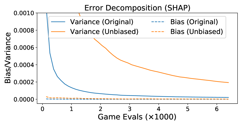
To facilitate our analysis of KernelSHAP, we present a simple experiment to compare the two estimators. We approximated the SHAP values for an individual prediction in the census income dataset [22] and empirically calculated the mean squared error relative to the true SHAP values across 250 runs. We then decomposed the error into bias and variance terms as follows:

$$\underbrace{\mathbb{E}\big{[}||\hat{\beta}_{n}-\beta^{*}||^{2}\big{]}}_{\text{Error}}=\underbrace{\mathbb{E}\big{[}||\hat{\beta}_{n}-\mathbb{E}[\hat{\beta}_{n}]||^{2}\big{]}}_{\text{Variance}}+\underbrace{\big{|}\big{|}\mathbb{E}[\hat{\beta}_{n}]-\beta^{*}\big{|}\big{|}^{2}.}_{\text{Bias}}$$

Figure 1 shows that the error for both estimators is dominated by variance rather than bias. It also shows that KernelSHAP incurs virtually no bias in exchange for significantly lower variance. In Appendix F, we provide global measures of the bias and variance to confirm these observations across multiple examples and two other datasets. This suggests that although KernelSHAP is more difficult to analyze theoretically, it should be used in practice because its bias is negligible and it converges faster.

Figure 1: SHAP error decomposition for the original and unbiased KernelSHAP estimators. The bias and variance are calculated empirically across 250 runs.

4.2 Variance Reduction via Paired Sampling

Having analyzed each estimator’s properties, we now consider whether their convergence can be accelerated. We propose a simple variance reduction technique that leads to significantly faster convergence in practice.

When sampling $n$ subsets according to the distribution $z_{i}\sim p(Z)$, we suggest a paired sampling strategy where each sample $z_{i}$ is paired with its complement $\mathbf{1}-z_{i}$. To show why this approach accelerates convergence, we focus on unbiased KernelSHAP, which is easier to analyze theoretically.

When estimating $b$ for unbiased KernelSHAP ($\bar{\beta}_{n}$), consider using the following modified estimator that combines $z_{i}$ with $\mathbf{1}-z_{i}$:

$$\check{b}_{n}=\frac{1}{2n}\sum_{i=1}^{n}\big{(}z_{i}v(z_{i})+(\mathbf{1}{-}z_{i})v(\mathbf{1}{-}z_{i})-v(\mathbf{0})\big{)}.$$ (14)

Substituting this into unbiased KernelSHAP (Eq. 9) yields a new estimator $\check{\beta}_{n}$ that preserves the properties of being both consistent and unbiased:

$$\check{\beta}_{n}=A^{-1}\Big{(}\check{b}_{n}-\mathbf{1}\frac{\mathbf{1}^{T}A^{-1}\check{b}_{n}-v(\mathbf{1})+v(\mathbf{0})}{\mathbf{1}^{T}A^{-1}\mathbf{1}}\Big{)}.$$ (15)

For games $v$ that satisfy a specific condition, we can guarantee that this sampling approach leads to $\check{\beta}_{n}$ having lower variance than $\bar{\beta}_{n}$, even when we account for $\check{b}_{n}$ requiring twice as many cooperative game evaluations as $\bar{b}_{n}$ (see proof in Appendix B).

Theorem 1.

The difference between the covariance matrices for the estimators $\bar{\beta}_{2n}$ and $\check{\beta}_{n}$ is given by

$$\mathrm{Cov}(\bar{\beta}_{2n})-\mathrm{Cov}(\check{\beta}_{n})=\frac{1}{2n}CG_{v}C^{T},$$

where $G_{v}$ is a property of the game $v$, defined as

$$G_{v}=-\mathrm{Cov}\Big{(}Zv(Z),(\mathbf{1}-Z)v(\mathbf{1}-Z)\Big{)}.$$

For sufficiently large $n$, $G_{v}\succeq 0$ guarantees that the Gaussian confidence ellipsoid $\bar{E}_{2n,\alpha}$ for $\bar{\beta}_{2n}$ contains the corresponding confidence ellipsoid $\check{E}_{n,\alpha}$ for $\check{\beta}_{n}$, or $\check{E}_{n,\alpha}\subseteq\bar{E}_{2n,\alpha}$, at any confidence level $\alpha\in(0,1)$.

Theorem 1 shows that $\check{\beta}_{n}$ is a more precise estimator than $\bar{\beta}_{2n}$ when the condition $G_{v}\succeq 0$ is satisfied (i.e., $G_{v}$ is positive semi-definite). This may not hold in the general case, but in Appendix B we show that a weaker condition holds for all games: the diagonal values of $G_{v}$ satisfy $(G_{v})_{ii}\geq 0$ for any game $v$. Geometrically, this weaker condition means that $\bar{E}_{2n,\alpha}$ extends beyond $\check{E}_{n,\alpha}$ in the axis-aligned directions.

Figure 2: Gaussian 95% confidence ellipsoids for two SHAP values in a census income prediction (from 250 runs). The estimators use an equal number of samples.

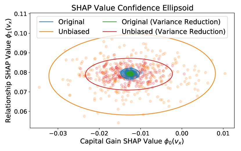
Figure 2 illustrates the result of Theorem 1 by showing empirical 95% confidence ellipsoids for two SHAP values. Although a comparable condition is difficult to derive for the original KernelSHAP estimator ($\hat{\beta}_{n}$), we find that the paired sampling approach yields a similar reduction in variance. Our experiments provide further evidence that this approach accelerates convergence for both estimators (Section 6).

4.3 Convergence Detection and Forecasting

One of KernelSHAP’s practical shortcomings is its lack of guidance on the number of samples required to obtain accurate estimates. We address this problem by developing an approach for convergence detection and forecasting.

Previously, we showed that unbiased KernelSHAP ($\bar{\beta}_{n}$) has variance that reduces at a rate $\mathcal{O}(\frac{1}{n})$ (Eq. 10). Furthermore, its variance is simple to estimate in practice: we require only an empirical estimate $\hat{\Sigma}_{\bar{b}}$ of $\Sigma_{\bar{b}}$ (defined above), which we can calculate using an online algorithm, such as Welford’s [42].

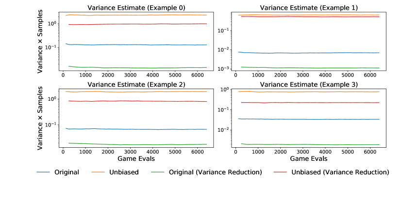
We also showed that the original KernelSHAP ($\hat{\beta}_{n}$) is difficult to characterize, but its variance is empirically lower than the unbiased version. Understanding its variance is useful for convergence detection, so we propose an approach for approximating it. Based on the results in Figure 1, we may hypothesize that KernelSHAP’s variance reduces at the same rate of $\mathcal{O}(\frac{1}{n})$; in Appendix F, we examine this by plotting the product of the variance and the number of samples over the course of estimation. We find that the product is constant as the sample number increases, which suggests that the $\mathcal{O}(\frac{1}{n})$ rate holds in practice. This property is difficult to prove formally, but it can be used for simple variance approximation.

When running KernelSHAP, we suggest estimating the variance by selecting an intermediate value $m$ such that $m<<n$ and calculating multiple independent estimates $\hat{\beta}_{m}$ while accumulating samples for $\hat{\beta}_{n}$. For any $n$, we can then approximate $\mathrm{Cov}(\hat{\beta}_{n})$ as

$$\mathrm{Cov}(\hat{\beta}_{n})\approx\frac{m}{n}\mathrm{Cov}(\hat{\beta}_{m}),$$

where $\mathrm{Cov}(\hat{\beta}_{m})$ is estimated empirically using the multiple independent estimates $\hat{\beta}_{m}$. This online approach has a negligible impact on the algorithm’s run-time, and the covariance estimate can be used to provide confidence intervals for the final results.

Whether we use the original or unbiased version of KernelSHAP, the estimator’s covariance at a given value of $n$ lets us both detect and forecast convergence. For detection, we propose stopping at the current value $n$ when the largest standard deviation is a sufficiently small portion $t$ (e.g., $t=0.01$) of the gap between the largest and smallest Shapley value estimates. For unbiased KernelSHAP, this criterion is equivalent to:

$$\max_{i}\sqrt{\frac{1}{n}(\hat{\Sigma}_{\bar{\beta}})_{ii}}<t\Big{(}\max_{i}\;(\bar{\beta}_{n})_{i}-\min_{i}\;(\bar{\beta}_{n})_{i}\Big{)}.$$

To forecast the number of samples required to reach convergence, we again invoke the property that estimates have variance that reduces at a rate of $\mathcal{O}(\frac{1}{n})$. Given a value $t$ and estimates $\bar{\beta}_{n}$ and $\hat{\Sigma}_{\bar{\beta}}$, the approximate number of samples $\hat{N}$ required is:

$$\hat{N}=\frac{1}{t^{2}}\Big{(}\frac{\max_{i}\;\sqrt{(\hat{\Sigma}_{\bar{\beta}})_{ii}}}{\max_{i}\;(\bar{\beta}_{n})_{i}-\min_{i}\;(\bar{\beta}_{n})_{i}}\Big{)}^{2}.$$

This allows us to forecast the time until convergence at any point during the algorithm. The forecast is expected to become more accurate as the estimated terms become more precise.

Our approach is theoretically grounded for unbiased KernelSHAP, and the approximate approach for the standard version of KernelSHAP relies only on the assumption that $\mathrm{Cov}(\hat{\beta}_{n})$ reduces at a rate of $\mathcal{O}(\frac{1}{n})$. Appendix G shows algorithms for both approaches, which illustrate both variance reduction and convergence detection techniques.

Figure 3: Shapley value-based explanations with 95% uncertainty estimates. Left: SHAP values for a single prediction with the census income dataset. Right: SAGE values for the German credit dataset.

5 STOCHASTIC COOPERATIVE GAMES

We have thus far focused on developing a regression-based approach to estimate Shapley values for any cooperative game. We now discuss how to adapt this approach to stochastic cooperative games, which leads to fast estimators for two global explanation methods.

5.1 Stochastic Cooperative Games

Stochastic cooperative games return a random value for each coalition of participating players $S\subseteq D$. Such games are represented by a function $V$ that maps coalitions to a distribution of possible outcomes, so that $V(S)$ is a random variable [9, 7].

To aid our presentation, we assume that the uncertainty in the game can be represented by an exogenous random variable $U$. The game can then be denoted by $V(S,U)$, where $V(\cdot,U)$ is a deterministic function of $S$ for any fixed value of the variable $U$.

Stochastic cooperative games provide a useful tool for understanding two global explanation methods, SAGE [12] and Shapley Effects [32]. To see why, assume an exogenous variable $U=(X,Y)$ that represents a random input-label pair, and consider the following game:

$$W(S,X,Y)=-\ell\Big{(}\mathbb{E}\big{[}f(X)|X_{S}\big{]},Y\Big{)}.$$ (16)

The game $W$ evaluates the (negated) loss with respect to the label $Y$ given a prediction that depends only on the features $X_{S}$. The cooperative game used by SAGE can be understood as the expectation of this game, or $w(S)=\mathbb{E}_{XY}\big{[}W(S,X,Y)\big{]}$ (see Eq. 2). Shapley Effects is based on the expectation of a similar game, where the loss is evaluated with respect to the full model prediction $f(X)$ (see Appendix C). As we show next, an approximation approach tailored to this setting yields significantly faster estimators for these methods.

5.2 Generalizing the Shapley Value

It is natural to assign values to players in stochastic cooperative games like we do for deterministic games. We propose a simple generalization of the Shapley value for games $V(S,U)$ that averages a player’s marginal contributions over both (i) player orderings and (ii) values of the exogenous variable $U$:

$$\phi_{i}(V)=\frac{1}{d}{\sum_{S{\subseteq}D{\setminus}\{i\}}}\binom{d{-}1}{|S|}^{{-}1}\mathbb{E}_{U}\Big{[}V(S\cup\{i\},U){-}V(S,U)\Big{]}.$$

Due to the linearity property of Shapley values [36, 30], the following sets of values are equivalent:

1. The Shapley values of the game’s expectation $\bar{v}(S)=\mathbb{E}_{U}[V(S,U)]$, or $\phi_{i}(\bar{v})$

2. The expected Shapley values of games with fixed $U$, or $\mathbb{E}_{U}[\phi_{i}(v_{U})]$ where $v_{u}(S)=V(S,u)$

3. Our generalization of Shapley values to the stochastic cooperative game $V(S,U)$, or $\phi_{i}(V)$

The first two list items suggest ways of calculating the values $\phi_{i}(V)$ using tools designed for deterministic cooperative games. However, the expectation $\mathbb{E}_{U}\big{[}V(S,U)\big{]}$ may be slow to evaluate (e.g., if it is across an entire dataset), and calculating Shapley values separately for each value of $U$ would be intractable if $U$ has many possible values. We therefore introduce a third approach.

5.3 Shapley Value Approximation for Stochastic Cooperative Games

We now propose a fast, regression-based approach for calculating the generalized Shapley values $\phi_{i}(V)$ of stochastic cooperative games $V(S,U)$. Fortunately, it requires only a simple modification of the preceding approaches.

Figure 4: Convergence forecasting for SHAP, Shapley Effects and SAGE. The required number of samples is compared with the predicted number across 100 runs (with 90% confidence intervals displayed).

First, we must calculate the values $\mathbb{E}_{U}\big{[}V(\mathbf{1},U)\big{]}$ and $\mathbb{E}_{U}\big{[}V(\mathbf{0},U)\big{]}$ for the grand coalition and the empty coalition. Next, we replace our previous $b$ estimators ($\hat{b}_{n}$ and $\bar{b}_{n}$) with estimators that use $n$ pairs of independent samples $z_{i}\sim p(Z)$ and $u_{i}\sim p(U)$. To adapt the original KernelSHAP to this setting, we use

$$\tilde{b}_{n}=\frac{1}{2}\sum_{i=1}^{n}z_{i}\big{(}V(z_{i},u_{i})-\mathbb{E}_{U}\big{[}V(\mathbf{0},U)\big{]}\big{)}.$$

We then substitute this into the KernelSHAP estimator, as follows:

$$\tilde{\beta}_{n}=\hat{A}_{n}^{-1}\Big{(}\tilde{b}_{n}-\mathbf{1}\frac{\mathbf{1}^{T}\hat{A}_{n}^{-1}\tilde{b}_{n}-v(\mathbf{1})+v(\mathbf{0})}{\mathbf{1}^{T}\hat{A}_{n}^{-1}\mathbf{1}}\Big{)}.$$ (17)

By the same argument used in Section 3.2, this approach estimates a solution to the weighted least squares problem whose optimal solution is the generalized Shapley values $\phi_{i}(V)$. This adaptation of KernelSHAP is consistent, and the analogous version of unbiased KernelSHAP is consistent and unbiased (see Appendix D). These can be run with our paired sampling approach, and we can also provide uncertainty estimates and detect convergence (Section 4).

6 EXPERIMENTS

We conducted experiments with four datasets to demonstrate the advantages of our Shapley value estimation approach. We used the census income dataset [22], the Portuguese bank marketing dataset [31], the German credit dataset [22], and a breast cancer (BRCA) subtype classification dataset [4]. To avoid overfitting with the BRCA data, we analyzed a random subset of 100 out of 17,814 genes (Appendix E). We trained a LightGBM model [21] for the census data, CatBoost [34] for the credit and bank data, and logistic regression for the BRCA data. Code for our experiments is available online.

Figure 5: Convergence acceleration for SAGE and Shapley Effects. The ratio of the maximum standard deviation to the gap between the largest and smallest Shapley values is compared across six estimators.

Table 1: SHAP estimator run-time comparison. Each value represents the ratio of the average number of samples required relative to the fastest estimator for that dataset (lower is better).

	Census Income	Bank Marketing	German Credit	BRCA Subtypes
Unbiased	380.63	176.45	17437.44	90.40
Unbiased + Paired Sampling	128.60	90.61	422.17	40.44
Original (KernelSHAP)	12.74	7.41	13.74	2.49
Original + Paired Sampling	1.00	1.00	1.00	1.00

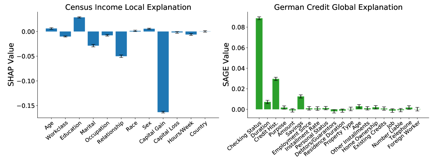
To demonstrate local and global explanations with uncertainty estimates, we show examples of SHAP [24] and SAGE [12] values generated using our estimators (Figure 3). Both explanations used a convergence threshold of $t=0.01$ and display 95% confidence intervals, which are features not previously offered by KernelSHAP. We used the dataset sampling approach for both explanations, and for SAGE we used the estimator designed for stochastic cooperative games. These estimators are faster than their unbiased versions, but the results are nearly identical.

To measure run-time differences between each estimator when calculating SHAP values, we compared the number of samples required to explain 100 instances for each dataset (Table 1). Rather than reporting the exact number of samples, which is dependent on the convergence threshold, we show the ratio between the number of samples required by each estimator; this ratio is independent of the convergence threshold when convergence is defined by the mean squared estimation error falling below a fixed value (Appendix E). Table 1 displays results based on 100 runs for each instance. Results show that the dataset sampling approach (original) is consistently faster than the unbiased estimator, and that paired sampling enables significantly faster convergence. In particular, we find that our paired sampling approach yields a $\mathbf{9\times}$ speedup on average over the original KernelSHAP.

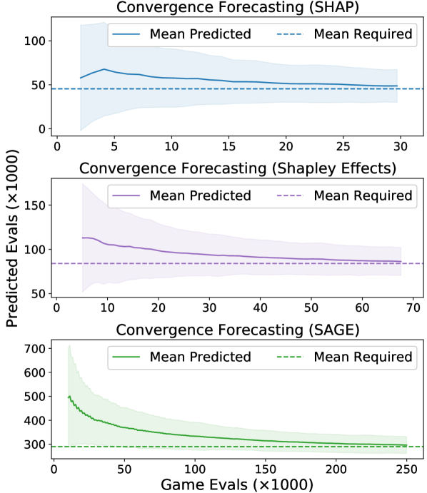
To investigate the accuracy of our convergence forecasting method, we compared the predicted number of samples to the true number across 250 runs. The number of samples depends on the convergence threshold, and we used a threshold $t=0.005$ for SHAP and $t=0.02$ for Shapley Effects and SAGE. Figure 4 shows the results for SHAP (using the census data), Shapley Effects (using the bank data) and SAGE (using the BRCA data). In all three cases, the forecasts become more accurate with more samples, and they vary within an increasingly narrow range around the true number of required samples. There is a positive bias in the forecast, but the bias diminishes with more samples.

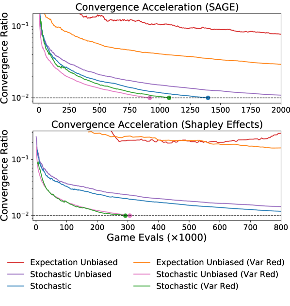
Finally, to demonstrate the speedup from our approach for stochastic cooperative games, we show that our stochastic estimator converges faster than a naive estimator based on the underlying game’s expectation (see Section 5.2). We plotted the ratio between the maximum standard deviation and the gap between the smallest and largest values, which we used to detect convergence (using a threshold $t=0.01$). Figure 5 shows that the stochastic approach dramatically speeds up both SAGE (using the BRCA data) and Shapley Effects (using the bank data), and that the paired sampling technique accelerates convergence for all estimators. The estimators based on the game’s expectation are prohibitively slow and could not be run to convergence. The fastest estimators for both datasets are stochastic estimators using the paired sampling technique, and only these methods converged for both datasets in the number of samples displayed. As is the case for SHAP, the dataset sampling approach is often faster than the unbiased approach, but the latter is slightly faster for SAGE when using paired sampling.

7 DISCUSSION

This paper described several approaches for estimating Shapley values via linear regression. We first introduced an unbiased version of KernelSHAP, with properties that are simpler to analyze than the original version. We then developed techniques for detecting convergence, calculating uncertainty estimates, and reducing the variance of both the original and unbiased estimators. Finally, we adapted our approach to provide significantly faster estimators for two global explanation methods based on stochastic cooperative games. Our work makes significant strides towards improving the practicality of Shapley value estimation by automatically determining the required number of samples, providing confidence intervals, and accelerating the estimation process.

More broadly, our work contributes to a mature literature on Shapley value estimation [6, 26] and to the growing ML model explanation field [32, 38, 13, 24, 12]. We focused on improving the regression-based approach to Shapley value estimation, and we leave to future work a detailed comparison of this approach to sampling-based [38, 37, 10, 12] and model-specific approximations [1, 25]. We also believe that certain insights from our work may be applicable to LIME, which is based on a similar dataset sampling approach; recent work has noted LIME’s high variance when using an insufficient number of samples [3], and an improved understanding of its convergence properties [16, 27] may lead to approaches for automatic convergence detection and uncertainty estimation.

Appendix A CALCULATING $A$ EXACTLY

Recall the definition of $A$, which is a term in the solution to the Shapley value linear regression problem:

$$A=\mathbb{E}[ZZ^{T}].$$

The entries of $A$ are straightforward to calculate because $Z$ is a random binary vector with a known distribution. Recall that $Z$ is distributed according to $p(Z)$, which is defined as:

$$p(z)=\begin{cases}Q^{-1}\mu_{\mathrm{Sh}}(Z)\quad 0<\mathbf{1}^{T}z<d\\ 0\quad\quad\quad\quad\quad\;\mathrm{otherwise},\end{cases}$$

where the normalizing constant $Q$ is given by:

$$Q =\sum_{0<\mathbf{1}^{T}z<d}\mu_{\mathrm{Sh}}(z)$$

$$=\sum_{k=1}^{d-1}\binom{d}{k}\frac{d-1}{\binom{d}{k}k(d-k)}$$

$$=(d-1)\sum_{k=1}^{d-1}\frac{1}{k(d-k)}.$$

Although $Q$ does not have a simple closed-form solution, the expression above can be calculated numerically. The diagonal entries $A_{ii}$ are then given by:

$$A_{ii} =\mathbb{E}[Z_{i}Z_{i}]=p(Z_{i}=1)$$

$$=\sum_{k=1}^{d-1}p(Z_{i}=1|\mathbf{1}^{T}Z=k)p(\mathbf{1}^{T}Z=k)$$

$$=\sum_{k=1}^{d-1}\frac{\binom{d-1}{k-1}}{\binom{d}{k}}\cdot Q^{-1}\binom{d}{k}\frac{d-1}{\binom{d}{k}k(d-k)}$$

$$=\frac{\sum_{k=1}^{d-1}\frac{1}{d(d-k)}}{\sum_{k=1}^{d-1}\frac{1}{k(d-k)}}.$$

This is equal to $\frac{1}{2}$ regardless of the value of $d$. To see this, consider the probability $p(Z_{i}=0)$:

$$p(Z_{i}=0) =1-p(Z_{i}=1)$$

$$=1-\frac{\sum_{k=1}^{d-1}\frac{1}{d(d-k)}}{\sum_{k=1}^{d-1}\frac{1}{k(d-k)}}$$

$$=\frac{\sum_{k=1}^{d-1}\frac{1}{d(d-k)}}{\sum_{k=1}^{d-1}\frac{1}{k(d-k)}}$$

$$=p(Z_{i}=1)$$

$$\Rightarrow A_{ii} =\frac{1}{2}.$$

Next, consider the off-diagonal entries $A_{ij}$ for $i\neq j$:

$$A_{ij} =\mathbb{E}[Z_{i}Z_{j}]=p(Z_{i}=Z_{j}=1)$$

$$=\sum_{k=2}^{d-1}p(Z_{i}=Z_{j}=1|\mathbf{1}^{T}Z=k)p(\mathbf{1}^{T}Z=k)$$

$$=\sum_{k=2}^{d-1}\frac{\binom{d-2}{k-2}}{\binom{d}{k}}\cdot Q^{-1}\binom{d}{k}\frac{d-1}{\binom{d}{k}k(d-k)}$$

$$=\frac{1}{d(d-1)}\frac{\sum_{k=2}^{d-1}\frac{k-1}{d-k}}{\sum_{k=1}^{d-1}\frac{1}{k(d-k)}}.$$

The value for off-diagonal entries $A_{ij}$ depends on $d$, unlike the diagonal entries $A_{ii}$. Although it does not have a simple closed-form expression, this value can be calculated numerically in $\mathcal{O}(d)$ time.

Appendix B VARIANCE REDUCTION PROOF

We present a proof for Theorem 1, and we prove that a weaker condition than $G_{v}\succeq 0$ holds for all cooperative games (the diagonal elements satisfy $(G_{v})_{ii}\geq 0$ for all games $v$).

B.1 Theorem 1 Proof

In Section 4.2, we proposed a variance reduction technique that pairs each sample $z_{i}\sim p(Z)$ with its complement $\mathbf{1}-z_{i}$ when estimating $b$. We now provide a proof for the condition that must be satisfied for the estimator $\check{\beta}_{n}$ to have lower variance than $\bar{\beta}_{n}$. As mentioned in the main text, the multivariate CLT asserts that

$$\bar{b}_{n}\sqrt{n} \xrightarrow{D}\mathcal{N}(b,\Sigma_{\bar{b}})$$

$$\check{b}_{n}\sqrt{n} \xrightarrow{D}\mathcal{N}(b,\Sigma_{\check{b}}),$$

where

$$\Sigma_{\bar{b}} =\mathrm{Cov}\big{(}Zv(Z)\big{)},$$

$$\Sigma_{\check{b}} =\mathrm{Cov}\Big{(}\frac{1}{2}\big{(}Zv(Z)+(\mathbf{1}-Z)v(\mathbf{1}-Z)\big{)}\Big{)}.$$

We can also apply the multivariate CLT to the Shapley value estimators $\bar{\beta}_{n}$ and $\check{\beta}_{n}$. We can see that

$$\bar{\beta}_{n}\sqrt{n} \xrightarrow{D}\mathcal{N}(\beta^{*},\Sigma_{\bar{\beta}})$$

$$\check{\beta}_{n}\sqrt{n} \xrightarrow{D}\mathcal{N}(\beta^{*},\Sigma_{\check{\beta}}),$$

where, due to their multiplicative dependence on $b$ estimators, the covariance matrices are defined as

$$\Sigma_{\bar{\beta}} =C\Sigma_{\bar{b}}C^{T}$$

$$\Sigma_{\check{\beta}} =C\Sigma_{\check{b}}C^{T}.$$

Next, we examine the relationship between $\Sigma_{\bar{b}}$ and $\Sigma_{\check{b}}$ because they dictate the relationship between $\Sigma_{\bar{\beta}}$ and $\Sigma_{\check{\beta}}$. To simplify our notation, we introduce three jointly distributed random variables, $M^{0}$, $M^{1}$ and $\bar{M}$, which are all functions of the random variable $Z$:

$$M^{0} =Zv(Z)-\mathbb{E}[Z]v(\mathbf{0})$$

$$M^{1} =(\mathbf{1}-Z)v(\mathbf{1}-Z)-\mathbb{E}[\mathbf{1}-Z]v(\mathbf{0})$$

$$\bar{M} =\frac{1}{2}\big{(}M^{0}+M^{1}\big{)}.$$

To understand $\bar{M}$’s covariance structure, we can decompose it using standard covariance properties and the fact that $p(z)=p(\mathbf{1}-z)$ for all $z$:

$$\mathrm{Cov}(\bar{M},\bar{M})_{ij} =\frac{1}{4}\mathrm{Cov}(M^{0}_{i}+M^{1}_{i},M^{0}_{j}+M^{1}_{j})$$

$$=\frac{1}{4}\Big{(}\mathrm{Cov}(M^{0}_{i},M^{0}_{j})+\mathrm{Cov}(M^{1}_{i},\bar{M}^{1}_{j})+\mathrm{Cov}(M^{0}_{i},M^{1}_{j})+\mathrm{Cov}(M^{1}_{i},M^{0}_{j})\Big{)}$$

$$=\frac{1}{2}\Big{(}\mathrm{Cov}(M^{0}_{i},M^{0}_{j})+\mathrm{Cov}(M^{0}_{i},M^{1}_{j})\Big{)}.$$

We can now compare $\Sigma_{\bar{b}}$ to $\Sigma_{\check{b}}$. To account for each $\bar{M}$ sample requiring twice as many cooperative game evaluations as $M^{0}$, we compare the covariance $\mathrm{Cov}(\bar{b}_{2n})$ to the covariance $\mathrm{Cov}(\check{b}_{n})$:

$$n\Big{(}\mathrm{Cov}(\bar{b}_{2n})-\mathrm{Cov}(\check{b}_{n})\Big{)}_{ij} =-\frac{1}{2}\mathrm{Cov}(M^{0}_{i},M^{1}_{j}).$$

Based on this, we define $G_{v}$ as follows:

$$G_{v} =-\mathrm{Cov}(M^{0}_{i},M^{1}_{j})$$

$$=-\mathrm{Cov}\Big{(}Zv(Z)-\mathbb{E}[Z]v(\mathbf{0}),(\mathbf{1}-Z)v(\mathbf{1}-Z)-\mathbb{E}[\mathbf{1}-Z]v(\mathbf{0})\Big{)}$$

$$=-\mathrm{Cov}\Big{(}Zv(Z),(\mathbf{1}-Z)v(\mathbf{1}-Z)\Big{)}.$$

This is the matrix referenced in Theorem 1. Notice that $G_{v}$ is the negated cross-covariance between $M^{0}$ and $M^{1}$, which is the off-diagonal block in the joint covariance matrix for the concatenated random variable $(M^{0},M^{1})$. This matrix is symmetric, unlike general cross-covariance matrices, and its eigen-structure determines whether our variance reduction approach is effective. In particular, if the condition $G_{v}\succeq 0$ is satisfied, then we have

$$\mathrm{Cov}(\bar{b}_{2n})\succeq\mathrm{Cov}(\check{b}_{n}),$$

which implies that

$$\mathrm{Cov}(\bar{\beta}_{2n})\succeq\mathrm{Cov}(\check{\beta}_{n}).$$

Since the inverses of two ordered matrices are also ordered, we get the result:

$$\mathrm{Cov}(\bar{\beta}_{2n})^{-1}\preceq\mathrm{Cov}(\check{\beta}_{n})^{-1}.$$

This has implications for quadratic forms involving each matrix. For any vector $a\in\mathbb{R}^{d}$, we have the inequality

$$a^{T}\mathrm{Cov}(\bar{\beta}_{2n})^{-1}a\leq a^{T}\mathrm{Cov}(\check{\beta}_{n})^{-1}a.$$

The last inequality has a geometric interpretation. It shows that the confidence ellipsoid (i.e., the confidence region, or prediction ellipsoid) for $\check{\beta}_{n}$ is contained by the corresponding confidence ellipsoid for $\bar{\beta}_{2n}$ since large values of $n$ lead each estimator to converge to its asymptotically normal distribution. This is because the confidence ellipsoids are defined for $\alpha\in(0,1)$ as

$$\bar{E}_{2n,\alpha}=\Big{\{}a\in\mathbb{R}^{d}:(a-\beta^{*})^{T}\mathrm{Cov}(\bar{\beta}_{2n})^{-1}(a-\beta^{*})\leq\sqrt{\chi^{2}_{d}(\alpha)}\Big{\}}$$

$$\check{E}_{n,\alpha}=\Big{\{}a\in\mathbb{R}^{d}:(a-\beta^{*})^{T}\mathrm{Cov}(\check{\beta}_{n})^{-1}(a-\beta^{*})\leq\sqrt{\chi^{2}_{d}(\alpha)}\Big{\}},$$

where $\chi^{2}_{d}(\alpha)$ denotes the inverse CDF of a Chi-squared distribution with $d$ degrees of freedom evaluated at $\alpha$. More precisely, we have $\check{E}_{n,\alpha}\subseteq\bar{E}_{2n,\alpha}$ because

$$(a-\beta^{*})^{T}\mathrm{Cov}(\check{\beta}_{n})^{-1}(a-\beta^{*})\leq\sqrt{\chi^{2}_{d}(\alpha)}$$

$$\Rightarrow (a-\beta^{*})^{T}\mathrm{Cov}(\bar{\beta}_{2n})^{-1}(a-\beta^{*})\leq\sqrt{\chi^{2}_{d}(\alpha)}.$$

This completes the proof.

B.2 A Weaker Condition

Consider the matrix $G_{v}$, which for a game $v$ is defined as

$$G_{v}=-\mathrm{Cov}\Big{(}Zv(Z),(\mathbf{1}-Z)v(\mathbf{1}-Z)\Big{)}.$$

A necessary (but not sufficient) condition for $G_{v}\succeq 0$ is that its diagonal elements are non-negative. We can prove that this weaker condition holds for all games. For an arbitrary game $v$, the diagonal value $(G_{v})_{ii}$ is given by:

$$(G_{v})_{ii} =-\mathrm{Cov}\Big{(}Z_{i}v(Z),(1-Z_{i})v(\mathbf{1}-Z)\Big{)}$$

$$=-\mathbb{E}\big{[}Z_{i}(1-Z_{i})v(Z)v(\mathbf{1}-Z)\big{]}+\mathbb{E}\big{[}Z_{i}v(Z)\big{]}\mathbb{E}\big{[}(1-Z_{i})v(\mathbf{1}-Z)\big{]}$$

$$=\mathbb{E}\big{[}Z_{i}v(Z)\big{]}^{2}$$

$$=\mathbb{E}\big{[}v(S)|i\in S\big{]}^{2}$$

$$\geq 0.$$

Geometrically, this condition means that the confidence ellipsoid $\bar{E}_{2n,\alpha}$ extends beyond the ellipsoid $\check{E}_{n,\alpha}$ in the axis-aligned directions. In a probabilistic sense, it means that the variance for each Shapley value estimate is lower when using the paired sampling technique.

Appendix C SHAPLEY EFFECTS

Shapley Effects is a model explanation method that summarizes the model $f$’s sensitivity to each feature [32]. It is based on the cooperative game

$$\tilde{w}(S)=\mathrm{Var}\big{(}\mathbb{E}[f(X)|X_{S}]\big{)}.$$ (18)

To show that Shapley Effects can be viewed as the expectation of a stochastic cooperative game, we reformulate this game (Covert et al. [12]) as:

$$\tilde{w}(S) =\mathrm{Var}\big{(}\mathbb{E}[f(X)|X_{S}]\big{)}$$

$$=\mathrm{Var}\big{(}f(X)\big{)}-\mathbb{E}_{X_{S}}\big{[}\mathrm{Var}(f(X)|X_{S})\big{]}$$

$$=c-\mathbb{E}_{X_{S}}\Big{[}\mathbb{E}_{X_{D\setminus S}|X_{S}}\big{[}\big{(}\mathbb{E}[f(X)|X_{S}]-f(X_{S},X_{D\setminus S})\big{)}^{2}\big{]}\Big{]}$$

$$=c-\mathbb{E}_{X}\Big{[}\big{(}\mathbb{E}[f(X)|X_{S}]-f(X)\big{)}^{2}\Big{]}.$$

If we generalize this cooperative game to allow arbitrary loss functions (e.g., cross entropy loss for classification tasks) rather than MSE, then we can ignore the constant value and re-write the game as

$$\tilde{w}(S)=-\mathbb{E}_{X}\Big{[}\ell\big{(}\mathbb{E}[f(X)|X_{S}],f(X)\big{)}\Big{]}.$$

Now, it is apparent that Shapley Effects is based on a cooperative game that is the expectation of a stochastic cooperative game, or $\tilde{w}(S)=\mathbb{E}_{X}[\tilde{W}(S,X)]$, where $\tilde{W}(S,X)$ is defined as:

$$\tilde{W}(S,X)=-\ell\big{(}\mathbb{E}[f(X)|X_{S}],f(X)\big{)}.$$

Unlike the stochastic cooperative game implicitly used by SAGE, the exogenous random variable for this game is $U=X$.

Appendix D STOCHASTIC COOPERATIVE GAME PROOFS

For a stochastic cooperative game $V(S,U)$, the generalized Shapley values are given by the expression

$$\phi_{i}(V) =\frac{1}{d}{\sum_{S{\subseteq}D{\setminus}\{i\}}}\binom{d{-}1}{|S|}^{{-}1}\mathbb{E}_{U}\big{[}V(S\cup\{i\},U){-}V(S,U)\big{]}$$

$$=\frac{1}{d}{\sum_{S{\subseteq}D{\setminus}\{i\}}}\binom{d{-}1}{|S|}^{{-}1}\mathbb{E}_{U}\big{[}V(S\cup\{i\},U)\big{]}-\mathbb{E}_{U}\big{[}V(S,U)\big{]}.$$

The second line above shows that the generalized Shapley values are equivalent to the Shapley values of the game’s expectation, or $\phi_{i}(\bar{V})$, where $\bar{V}(S)=\mathbb{E}_{U}[V(S,U)]$. Based on this, we can also understand the values $\phi_{1}(V),\ldots,\phi_{d}(V)$ as the optimal coefficients for the following weighted least squares problem:

$$\min_{\beta_{0},\ldots,\beta_{d}}\;\sum_{z}p(z)\Big{(}\beta_{0}+z^{T}\beta-\mathbb{E}_{U}\big{[}V(z,U)\big{]}\Big{)}^{2}$$

$$\mathrm{s.t.}\quad\beta_{0}=\mathbb{E}_{U}\big{[}V(\mathbf{0},U)\big{]},\quad\mathbf{1}^{T}\beta=\mathbb{E}_{U}\big{[}V(\mathbf{1},U)\big{]}-\mathbb{E}_{U}\big{[}V(\mathbf{0},U)\big{]}.$$

Using our derivation from the main text (Section 3.3), we can write the solution as

$$\beta^{*}=A^{-1}\Big{(}b-\mathbf{1}\frac{\mathbf{1}^{T}A^{-1}b-\mathbb{E}_{U}[V(\mathbf{1},U)]+\mathbb{E}_{U}[V(\mathbf{0},U)]}{\mathbf{1}^{T}A^{-1}\mathbf{1}}\Big{)},$$

where $A$ and $b$ are given by the expressions

$$A =\mathbb{E}[ZZ^{T}]$$

$$b =\mathbb{E}_{Z}\Big{[}Z\big{(}\mathbb{E}_{U}[V(Z,U)]-\mathbb{E}_{U}[V(\mathbf{0},U)]\big{)}\Big{]}.$$

Now, we consider our adaptations of KernelSHAP and unbiased KernelSHAP and examine whether these estimators are consistent or unbiased. We begin with the stochastic version of KernelSHAP presented in the main text (Section 5.3). Recall that this approach uses the original $A$ estimator $\hat{A}_{n}$ and the modified $b$ estimator $\tilde{b}_{n}$, which is defined as:

$$\tilde{b}_{n}=\frac{1}{2}\sum_{i=1}^{n}z_{i}\big{(}V(z_{i},u_{i})-\mathbb{E}_{U}\big{[}V(\mathbf{0},U)\big{]}\big{)}.$$

As mentioned in the main text, the strong law of large numbers lets us conclude that $\lim_{n\to\infty}\hat{A}_{n}=A$. Thus, we can understand the $b$ estimator’s expectation as follows:

$$\mathbb{E}\big{[}\tilde{b}_{n}\big{]} =\mathbb{E}_{ZU}\Big{[}Z\big{(}V(Z,U)-\mathbb{E}_{U}\big{[}V(\mathbf{0},U)\big{]}\big{)}\Big{]}$$

$$=\mathbb{E}_{Z}\Big{[}Z\big{(}\mathbb{E}_{U}[V(Z,U)]-\mathbb{E}_{U}[V(\mathbf{0},U)]\big{)}\Big{]}$$

$$=b.$$

With this, we conclude that $\lim_{n\to\infty}\tilde{b}_{n}=b$ and that $\tilde{\beta}_{n}$ are consistent, or

$$\lim_{n\to\infty}\tilde{\beta}_{n}=\beta^{*}.$$

To adapt unbiased KernelSHAP to the setting of stochastic cooperative games, we use the same technique of pairing independent samples of $Z$ and $U$. To estimate $b$, we use an estimator $\tilde{\bar{b}}_{n}$ defined as:

$$\tilde{\bar{b}}_{n}=\frac{1}{n}\sum_{i=1}^{n}z_{i}V(z_{i},u_{i})-\mathbb{E}\big{[}Z\big{]}\mathbb{E}_{U}\big{[}V(\mathbf{0},U)\big{]}.$$

We then substitute this into a Shapley value estimator as follows:

$$\tilde{\bar{\beta}}_{n}=A^{-1}\Big{(}\tilde{\bar{b}}_{n}-\mathbf{1}\frac{\mathbf{1}^{T}A^{-1}\tilde{\bar{b}}_{n}-v(\mathbf{1})+v(\mathbf{0})}{\mathbf{1}^{T}A^{-1}\mathbf{1}}\Big{)}.$$ (19)

This is consistent and unbiased because of the linear dependence on $\tilde{\bar{b}}_{n}$ and the fact that $\tilde{\bar{b}}_{n}$ is unbiased:

$$\mathbb{E}\big{[}\tilde{\bar{b}}_{n}\big{]} =\mathbb{E}_{ZU}\Big{[}ZV(Z,U)-\mathbb{E}\big{[}Z\big{]}\mathbb{E}_{U}\big{[}V(\mathbf{0},U)\big{]}\Big{]}$$

$$=\mathbb{E}_{Z}\Big{[}Z\big{(}\mathbb{E}_{U}[V(Z,U)]-\mathbb{E}_{U}[V(\mathbf{0},U)]\big{)}\Big{]}$$

$$=b.$$

With this, we conclude that $\mathbb{E}[\tilde{\bar{\beta}}_{n}]=\beta^{*}$ and $\lim_{n\to\infty}\tilde{\bar{\beta}}_{n}=\beta^{*}$.

Appendix E EXPERIMENT DETAILS

Here, we provide further details about experiments described in the main body of text.

E.1 Datasets and Hyperparameters

For all three explanation methods considered in our experiments – SHAP [24], SAGE [12] and Shapley Effects [32] – we handled removed features by marginalizing them out according to their joint marginal distribution. This is the default behavior for SHAP, but it is an approximation of what is required by SAGE and Shapley Effects. However, this choice should not affect the outcome of our experiments, which focus on the convergence properties of our Shapley value estimators (and not the underlying cooperative games).

Both SAGE and Shapley Effects require a loss function (Section C). We used the cross entropy loss for SAGE and the soft cross entropy loss for Shapley Effects.

For the breast cancer (BRCA) subtype classification dataset, we selected 100 out of 17,814 genes to avoid overfitting on the relatively small dataset size (only 510 patients). These genes were selected at random: we tried ten random seeds and selected the subset that achieved the best performance to ensure that several relevant BRCA genes were included. A small portion of missing expression values were imputed with their mean. The data was centered and normalized prior to fitting a $\ell_{1}$ regularized logistic regression model; the regularization parameter was chosen using a validation set.

E.2 SHAP Run-time Comparison

To compare the run-time of various SHAP value estimators, we sought to compare the ratio of the mean number of samples required by each method. For a single example $x$ whose SHAP values are represented by $\beta^{*}$, the mean squared estimation error can be decomposed into the variance and bias as follows:

$$\mathbb{E}\big{[}||\hat{\beta}_{n}-\beta^{*}||^{2}\big{]}=\mathbb{E}\big{[}||\hat{\beta}_{n}-\mathbb{E}[\hat{\beta}_{n}]||^{2}\big{]}+\big{|}\big{|}\mathbb{E}[\hat{\beta}_{n}]-\beta^{*}\big{|}\big{|}^{2}.$$

Since we found that the error is dominated by variance rather than bias (Section 4.1), we can make the following approximation to relate the error to the trace of the covariance matrix:

$$\mathbb{E}\big{[}||\hat{\beta}_{n}-\beta^{*}||^{2}\big{]} =\mathbb{E}\big{[}||\hat{\beta}_{n}-\mathbb{E}[\hat{\beta}_{n}]||^{2}\big{]}+\big{|}\big{|}\mathbb{E}[\hat{\beta}_{n}]-\beta^{*}\big{|}\big{|}^{2}$$

$$\approx\mathbb{E}\big{[}||\hat{\beta}_{n}-\mathbb{E}[\hat{\beta}_{n}]||^{2}\big{]}$$

$$=\operatorname{Tr}\Big{(}\mathrm{Cov}(\hat{\beta}_{n})\Big{)}.$$ (20)

If we define convergence based on the mean estimation error falling below a threshold value $t$, then the convergence condition is

$$\mathbb{E}\big{[}||\hat{\beta}_{n}-\beta^{*}||^{2}\big{]}\leq t.$$

Using our approximation (Eq. 20), we can see that this condition is approximately equivalent to

$$\mathbb{E}\big{[}||\hat{\beta}_{n}-\beta^{*}||^{2}\big{]}\approx\operatorname{Tr}\Big{(}\mathrm{Cov}(\hat{\beta}_{n})\Big{)}\approx\frac{\operatorname{Tr}(\Sigma_{\hat{\beta}})}{n}\leq t.$$

For a given threshold $t$, the mean number of samples required to explain individual predictions is therefore based on the mean trace of the covariance matrix $\Sigma_{\hat{\beta}}$ (or the analogous covariance matrix for a different estimator). To compare two methods, we simply calculate the ratio of the mean trace of the covariance matrices. These ratios are reported in Table 1, where each covariance matrix is calculated empirically across 100 runs with $n=2048$ samples.

Appendix F CONVERGENCE EXPERIMENTS

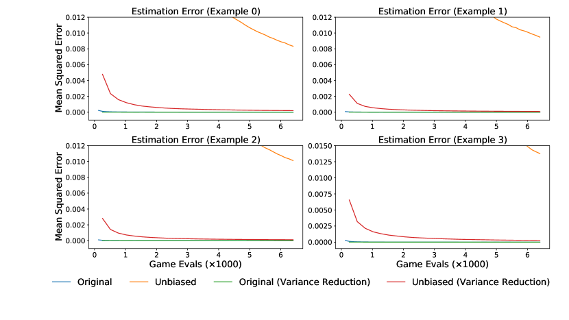
In Section 4.1, we empirically compared the bias and variance for the original and unbiased versions of KernelSHAP using a single census income prediction. The results (Figure 1) showed that both versions’ estimation errors were dominated by variance rather than bias, and that the original version had significantly lower variance. To verify that this result is not an anomaly, we replicated it on multiple examples and across several datasets.

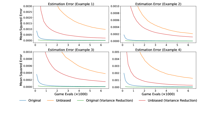
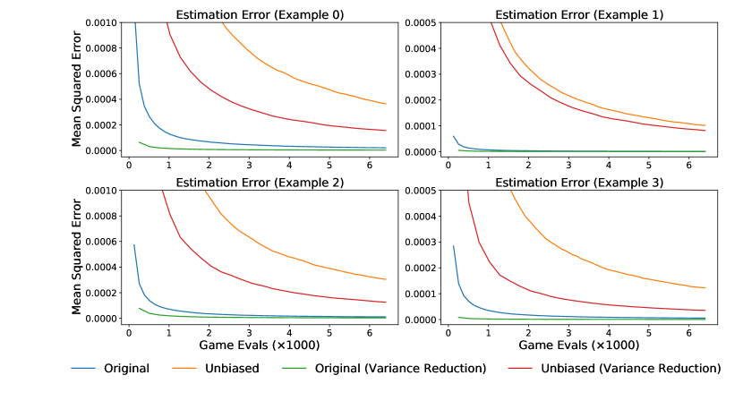
First, we examined several individual predictions for the census income, German credit and bank marketing datasets. To highlight the effectiveness of our paired sampling approach (Section 4.2), we added these methods as additional comparisons. Rather than decomposing the error into bias and variance as in the main text, we simply calculated the mean squared error across 100 runs of each estimator. Figure 7 shows the error for several census income predictions, Figure 9 for several bank marketing predictions, and Figure 11 for several credit quality predictions. These results confirm that the original version of KernelSHAP converges significantly faster than the unbiased version, and that the paired sampling technique is effective for both estimators. The dataset sampling approach (original KernelSHAP) appears preferable in practice despite being more difficult to analyze because it converges to the correct result much faster.

Second, we calculated a global measure of the bias and variance for each estimator using the same datasets (Table 2). Given 100 examples from each dataset, we calculated the mean bias and mean variance for each estimator empirically across 100 runs given $n=256$ samples. Results show that the bias is nearly zero for all estimators, not just the unbiased ones; they also show that the variance is often significantly larger than the bias. However, when using the dataset sampling approach (original) in combination with the paired sampling technique, the bias and variance are comparably low ($\approx 0$) after 256 samples. The only exception is the unbiased estimator that does not use paired sampling, but this is likely due to estimation error because its bias is provably equal to zero.

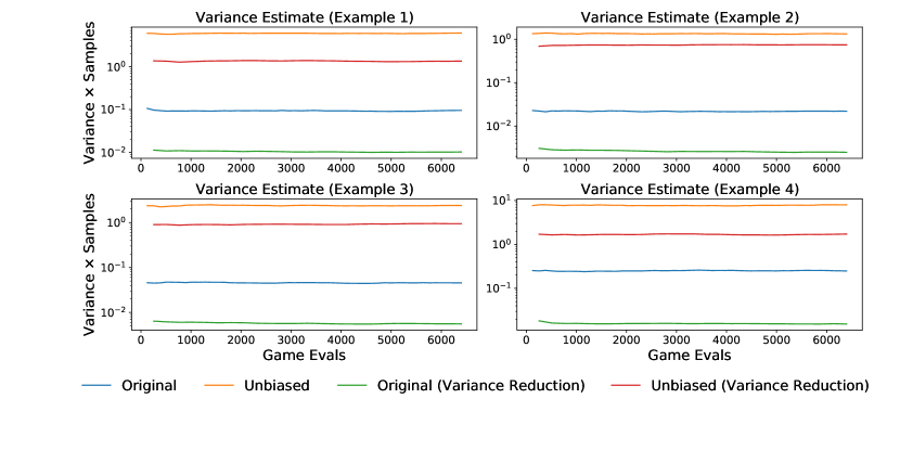
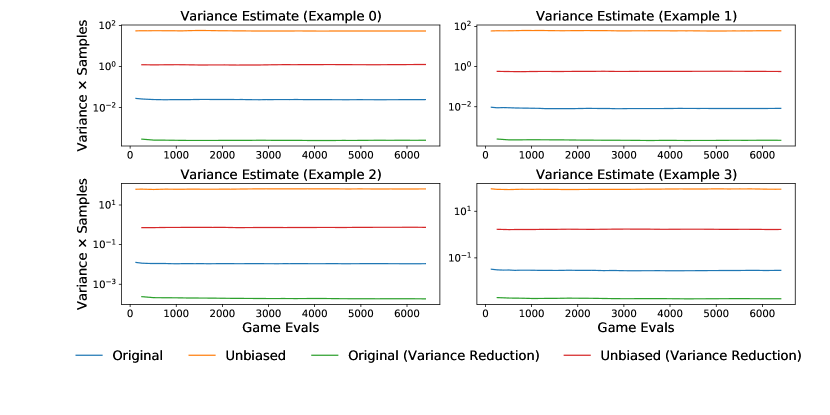
Finally, Section 4.3 also proposed assuming that the original KernelSHAP estimator’s variance reduces at a rate of $\mathcal{O}(\frac{1}{n})$, similar to the unbiased version (for which we proved this rate). Although this result is difficult to prove formally, it seems to hold empirically across multiple predictions and several datasets. In Figures 7,  9 and  11, we display the product of the estimator’s variance with the number of samples for the census, bank and credit datasets. Results confirm that the product is roughly constant as the number of samples increases, indicating that the variance for all four estimators (not just the unbiased ones) reduces at a rate of $\mathcal{O}(\frac{1}{n})$.

Table 2: Global measures of bias and variance for each SHAP value estimator. Each entry is the mean bias and mean variance calculated empirically across 100 examples (bias/variance, lower is better).

	Census Income	Bank Marketing	German Credit
Unbiased	0.0002/0.0208	0.0001/0.0125	0.0026/0.2561
Unbiased + Paired Sampling	0.0000/0.0068	0.0000/0.0066	0.0000/0.0062
Original (KernelSHAP)	0.0000/0.0007	0.0000/0.0006	0.0000/0.0002
Original + Paired Sampling	0.0000/0.0001	0.0000/0.0001	0.0000/0.0000

Figure 6: Census income SHAP value estimation error on four predictions.

Figure 7: Census income SHAP value variance estimation on four predictions.

Figure 8: Bank marketing SHAP value estimation error on four predictions.

Figure 9: Bank marketing SHAP value variance estimation on four predictions.

Figure 10: German credit SHAP value estimation error on four predictions.

Figure 11: German credit SHAP value variance estimation on four predictions.

Appendix G ALGORITHMS

Here, we provide pseudocode for the estimation algorithms described in the main text. Algorithm 1 shows the dataset sampling approach (original KernelSHAP) with our convergence detection and paired sampling techniques. Algorithm 2 shows KernelSHAP’s adaptation to the setting of stochastic cooperative games (stochastic KernelSHAP). Algorithm 3 shows the unbiased KernelSHAP estimator, and Algorithm 4 shows the adaptation of unbiased KernelSHAP to stochastic cooperative games.

Input: Game $v$, convergence threshold $t$, intermediate samples $m$

// Initialize

n = 0

A = 0

b = 0

// For tracking intermediate samples

counter = 0

Atemp = 0

btemp = 0

estimates = list()

// Sampling loop

converged = False

while not converged do

       // Draw next sample

       Sample $z\sim p(Z)$

       if variance reduction then

             Asample = $\frac{1}{2}\big{(}zz^{T}+(\mathbf{1}-z)(\mathbf{1}-z)^{T}\big{)}$

             bsample = $\frac{1}{2}\big{(}zv(z)+(\mathbf{1}{-}z)v(\mathbf{1}{-}z)-v(\mathbf{0})\big{)}$

            

       else

             Asample = $zz^{T}$

             bsample = $z\big{(}v(z)-v(\mathbf{0})\big{)}$

            

      

       // Welford’s algorithm

       n = n + 1

       A += (Asample $-$ A) / n

       b += (bsample $-$ b) / n

       counter += 1

       Atemp += (Asample $-$ Atemp) / counter

       btemp += (bsample $-$ btemp) / counter

      

       if counter == $m$ then

             // Get intermediate estimate

             $\beta_{m}=\mathrm{Atemp}^{-1}\Big{(}\mathrm{btemp}-\mathbf{1}\frac{\mathbf{1}^{T}\mathrm{Atemp}^{-1}\mathrm{btemp}-v(\mathbf{1})+v(\mathbf{0})}{\mathbf{1}^{T}\mathrm{Atemp}^{-1}\mathbf{1}}\Big{)}$

             estimates.append($\beta_{m}$)

             counter = 0

             Atemp = 0

             btemp = 0

            

             // Get estimates, uncertainties

             $\beta_{n}=\mathrm{A}^{-1}\Big{(}\mathrm{b}-\mathbf{1}\frac{\mathbf{1}^{T}\mathrm{A}^{-1}\mathrm{b}-v(\mathbf{1})+v(\mathbf{0})}{\mathbf{1}^{T}\mathrm{A}^{-1}\mathbf{1}}\Big{)}$

             $\Sigma_{\beta}=m\cdot\mathrm{Cov}(\mathrm{estimates})$ // Empirical covariance

             $\sigma_{n}=\sqrt{\mathrm{diag}(\Sigma_{\beta})/\mathrm{n}}$ // Element-wise square root

            

             // Check for convergence

             converged = $\Big{(}\frac{\max(\sigma_{n})}{\max(\beta_{n})-\min(\beta_{n})}<t$ )

            

      

end while

return $\beta_{n}$, $\sigma_{n}$

Algorithm 1 Shapley value estimation with dataset sampling (KernelSHAP)

Input: Game $V$, convergence threshold $t$, intermediate samples $m$

// Initialize

n = 0

A = 0

b = 0

// For tracking intermediate samples

counter = 0

Atemp = 0

btemp = 0

estimates = list()

// Sampling loop

converged = False

while not converged do

       // Draw next sample

       Sample $z\sim p(Z)$

       Sample $u\sim p(U)$

       if variance reduction then

             bsample = $\frac{1}{2}\big{(}zV(z,u)+(\mathbf{1}{-}z)V(\mathbf{1}{-}z,u)-\mathbb{E}_{U}[V(\mathbf{0},U)]\big{)}$

             Asample = $\frac{1}{2}\big{(}zz^{T}+(\mathbf{1}-z)(\mathbf{1}-z)^{T}\big{)}$

            

       else

             bsample = $z\big{(}V(z,u)-\mathbb{E}_{U}[V(\mathbf{0},U)]\big{)}$

             Asample = $zz^{T}$

            

      

       // Welford’s algorithm

       n = n + 1

       b += (bsample $-$ b) / n

       A += (Asample $-$ A) / n

       counter += 1

       btemp += (bsample $-$ btemp) / counter

       Atemp += (Asample $-$ Atemp) / counter

      

       if counter == $m$ then

             // Get intermediate estimate

             $\beta_{m}=\mathrm{Atemp}^{-1}\Big{(}\mathrm{btemp}-\mathbf{1}\frac{\mathbf{1}^{T}\mathrm{Atemp}^{-1}\mathrm{btemp}-\mathbb{E}_{U}[V(\mathbf{1},U)]+\mathbb{E}_{U}[V(\mathbf{0},U)]}{\mathbf{1}^{T}\mathrm{Atemp}^{-1}\mathbf{1}}\Big{)}$

             estimates.append($\beta_{m}$)

             counter = 0

             Atemp = 0

             btemp = 0

            

             // Get estimates, uncertainties

             $\beta_{n}=\mathrm{A}^{-1}\Big{(}\mathrm{b}-\mathbf{1}\frac{\mathbf{1}^{T}\mathrm{A}^{-1}\mathrm{b}-\mathbb{E}_{U}[V(\mathbf{1},U)]+\mathbb{E}_{U}[V(\mathbf{0},U)]}{\mathbf{1}^{T}\mathrm{A}^{-1}\mathbf{1}}\Big{)}$

             $\Sigma_{\beta}=m\cdot\mathrm{Cov}(\mathrm{estimates})$ // Empirical covariance

             $\sigma_{n}=\sqrt{\mathrm{diag}(\Sigma_{\beta})/\mathrm{n}}$ // Element-wise square root

            

             // Check for convergence

             converged = $\Big{(}\frac{\max(\sigma_{n})}{\max(\beta_{n})-\min(\beta_{n})}<t$ )

            

      

end while

return $\beta_{n}$, $\sigma_{n}$

Algorithm 2 Shapley value estimation with dataset sampling for stochastic cooperative games

Input: Game $v$, convergence threshold $t$

// Initialize

Set $A$ (Section 3.3)

Set $C$ (Eq. 13)

n = 0

b = 0

bSSQ = 0

// Sampling loop

converged = False

while not converged do

       // Draw next sample

       Sample $z\sim p(Z)$

       if variance reduction then

             bsample = $\frac{1}{2}\big{(}zv(z)+(\mathbf{1}{-}z)v(\mathbf{1}{-}z)-v(\mathbf{0})\big{)}$

            

       else

             bsample = $zv(z)-\frac{1}{2}v(\mathbf{0})$

            

      

       // Welford’s algorithm

       n = n + 1

       diff = (bsample $-$ b)

       b += diff / n

       diff2 = (bsample $-$ b)

       bSSQ += outer(diff, diff2) // Outer product

      

       // Get estimates, uncertainties

       $\beta_{n}=A^{-1}\Big{(}\mathrm{b}-\mathbf{1}\frac{\mathbf{1}^{T}A^{-1}\mathrm{b}-v(\mathbf{1})+v(\mathbf{0})}{\mathbf{1}^{T}A^{-1}\mathbf{1}}\Big{)}$

       $\Sigma_{b}=$ bSSQ / n

       $\Sigma_{\beta}=C\Sigma_{b}C^{T}$

       $\sigma_{n}=\sqrt{\mathrm{diag}(\Sigma_{\beta})/\mathrm{n}}$ // Element-wise square root

      

       // Check for convergence

       converged = $\Big{(}\frac{\max(\sigma_{n})}{\max(\beta_{n})-\min(\beta_{n})}<t$ )

      

end while

return $\beta_{n}$, $\sigma_{n}$

Algorithm 3 Unbiased Shapley value estimation

Input: Game $V$, convergence threshold $t$

// Initialize

Set $A$ (Section 3.3)

Set $C$ (Eq. 13)

n = 0

b = 0

bSSQ = 0

// Sampling loop

converged = False

while not converged do

       // Draw next sample

       Sample $z\sim p(Z)$

       Sample $u\sim p(U)$

       if variance reduction then

             bsample = $\frac{1}{2}\Big{(}zV(z,u)+(\mathbf{1}{-}z)V(\mathbf{1}{-}z,u)-\mathbb{E}_{U}\big{[}V(\mathbf{0}),U\big{]}\Big{)}$

            

       else

             bsample = $zV(z,u)-\frac{1}{2}\mathbb{E}_{U}[V(\mathbf{0},U)]$

            

      

       // Welford’s algorithm

       n = n + 1

       diff = (bsample $-$ b)

       b += diff / n

       diff2 = (bsample $-$ b)

       bSSQ += outer(diff, diff2) // Outer product

      

       // Get estimates, uncertainties

       $\beta_{n}=A^{-1}\Big{(}\mathrm{b}-\mathbf{1}\frac{\mathbf{1}^{T}A^{-1}\mathrm{b}-\mathbb{E}_{U}[V(\mathbf{1},U)]+\mathbb{E}_{U}[V(\mathbf{0},U)]}{\mathbf{1}^{T}A^{-1}\mathbf{1}}\Big{)}$

       $\Sigma_{b}=$ bSSQ / n

       $\Sigma_{\beta}=C\Sigma_{b}C^{T}$

       $\sigma_{n}=\sqrt{\mathrm{diag}(\Sigma_{\beta})/\mathrm{n}}$ // Element-wise square root

      

       // Check for convergence

       converged = $\Big{(}\frac{\max(\sigma_{n})}{\max(\beta_{n})-\min(\beta_{n})}<t$ )

      

end while

return $\beta_{n}$, $\sigma_{n}$

Algorithm 4 Unbiased Shapley value estimation for stochastic cooperative games

Acknowledgements

This work was funded by the National Science Foundation [CAREER DBI-1552309, and DBI- 1759487]; the American Cancer Society [127332-RSG-15-097-01-TBG]; and the National Institutes of Health [R35 GM 128638, and R01 NIA AG 061132]. We would like to thank Hugh Chen, the Lee Lab, and our AISTATS reviewers for feedback that greatly improved this work.

References

- Ancona et al. [2019] Marco Ancona, Cengiz Öztireli, and Markus Gross. Explaining deep neural networks with a polynomial time algorithm for Shapley values approximation. arXiv preprint arXiv:1903.10992, 2019.
- Aumann [1994] Robert JJ Aumann. Economic applications of the Shapley value. In Game-Theoretic Methods in General Equilibrium Analysis, pages 121–133. Springer, 1994.
- Bansal et al. [2020] Naman Bansal, Chirag Agarwal, and Anh Nguyen. SAM: The sensitivity of attribution methods to hyperparameters. In Proceedings of the IEEE/CVF Conference on Computer Vision and Pattern Recognition, pages 8673–8683, 2020.
- Berger et al. [2018] Ashton C Berger, Anil Korkut, Rupa S Kanchi, Apurva M Hegde, Walter Lenoir, Wenbin Liu, Yuexin Liu, Huihui Fan, Hui Shen, Visweswaran Ravikumar, et al. A comprehensive pan-cancer molecular study of gynecologic and breast cancers. Cancer Cell, 33(4):690–705, 2018.
- Boyd and Vandenberghe [2004] Stephen Boyd and Lieven Vandenberghe. Convex Optimization. Cambridge University Press, 2004.
- Castro et al. [2009] Javier Castro, Daniel Gómez, and Juan Tejada. Polynomial calculation of the Shapley value based on sampling. Computers & Operations Research, 36(5):1726–1730, 2009.
- Charnes and Granot [1976] A Charnes and Daniel Granot. Coalitional and chance-constrained solutions to n-person games. i: The prior satisficing nucleolus. SIAM Journal on Applied Mathematics, 31(2):358–367, 1976.
- Charnes et al. [1988] A Charnes, B Golany, M Keane, and J Rousseau. Extremal principle solutions of games in characteristic function form: core, Chebychev and Shapley value generalizations. In Econometrics of Planning and Efficiency, pages 123–133. Springer, 1988.
- Charnes and Granot [1973] Abraham Charnes and Daniel Granot. Prior solutions: Extensions of convex nucleus solutions to chance-constrained games. Technical report, Texas University at Austin Center for Cybernetic Studies, 1973.
- Chen et al. [2018] Jianbo Chen, Le Song, Martin J Wainwright, and Michael I Jordan. L-Shapley and C-Shapley: Efficient model interpretation for structured data. arXiv preprint arXiv:1808.02610, 2018.
- Covert et al. [2020a] Ian Covert, Scott Lundberg, and Su-In Lee. Explaining by removing: A unified framework for model explanation. arXiv preprint arXiv:2011.14878, 2020a.
- Covert et al. [2020b] Ian Covert, Scott Lundberg, and Su-In Lee. Understanding global feature contributions with additive importance measures. Advances in Neural Information Processing Systems, 34, 2020b.
- Datta et al. [2016] Anupam Datta, Shayak Sen, and Yair Zick. Algorithmic transparency via quantitative input influence: Theory and experiments with learning systems. In 2016 IEEE Symposium on Security and Privacy (SP), pages 598–617. IEEE, 2016.
- Ding et al. [2008] Guoli Ding, Robert F Lax, Jianhua Chen, and Peter P Chen. Formulas for approximating pseudo-boolean random variables. Discrete Applied Mathematics, 156(10):1581–1597, 2008.
- Ding et al. [2010] Guoli Ding, Robert F Lax, Jianhua Chen, Peter P Chen, and Brian D Marx. Transforms of pseudo-boolean random variables. Discrete Applied Mathematics, 158(1):13–24, 2010.
- Garreau and von Luxburg [2020] Damien Garreau and Ulrike von Luxburg. Looking deeper into LIME. arXiv preprint arXiv:2008.11092, 2020.
- Ghorbani and Zou [2019] Amirata Ghorbani and James Zou. Data Shapley: Equitable valuation of data for machine learning. arXiv preprint arXiv:1904.02868, 2019.
- Ghorbani and Zou [2020] Amirata Ghorbani and James Zou. Neuron Shapley: Discovering the responsible neurons. arXiv preprint arXiv:2002.09815, 2020.
- Grabisch et al. [2000] Michel Grabisch, Jean-Luc Marichal, and Marc Roubens. Equivalent representations of set functions. Mathematics of Operations Research, 25(2):157–178, 2000.
- Hammer and Holzman [1992] Peter L Hammer and Ron Holzman. Approximations of pseudo-boolean functions; applications to game theory. Zeitschrift für Operations Research, 36(1):3–21, 1992.
- Ke et al. [2017] Guolin Ke, Qi Meng, Thomas Finley, Taifeng Wang, Wei Chen, Weidong Ma, Qiwei Ye, and Tie-Yan Liu. Lightgbm: A highly efficient gradient boosting decision tree. In Advances in Neural Information Processing Systems, pages 3146–3154, 2017.
- Lichman et al. [2013] Moshe Lichman et al. UCI machine learning repository, 2013.
- Lipovetsky and Conklin [2001] Stan Lipovetsky and Michael Conklin. Analysis of regression in game theory approach. Applied Stochastic Models in Business and Industry, 17(4):319–330, 2001.
- Lundberg and Lee [2017] Scott M Lundberg and Su-In Lee. A unified approach to interpreting model predictions. In Advances in Neural Information Processing Systems, pages 4765–4774, 2017.
- Lundberg et al. [2020] Scott M Lundberg, Gabriel Erion, Hugh Chen, Alex DeGrave, Jordan M Prutkin, Bala Nair, Ronit Katz, Jonathan Himmelfarb, Nisha Bansal, and Su-In Lee. From local explanations to global understanding with explainable AI for trees. Nature Machine Intelligence, 2(1):2522–5839, 2020.
- Maleki et al. [2013] Sasan Maleki, Long Tran-Thanh, Greg Hines, Talal Rahwan, and Alex Rogers. Bounding the estimation error of sampling-based Shapley value approximation. arXiv preprint arXiv:1306.4265, 2013.
- Mardaoui and Garreau [2020] Dina Mardaoui and Damien Garreau. An analysis of LIME for text data. arXiv preprint arXiv:2010.12487, 2020.
- Marichal and Mathonet [2011] Jean-Luc Marichal and Pierre Mathonet. Weighted Banzhaf power and interaction indexes through weighted approximations of games. European Journal of Operational Research, 211(2):352–358, 2011.
- Merrick and Taly [2019] Luke Merrick and Ankur Taly. The explanation game: Explaining machine learning models using Shapley values. arXiv preprint arXiv:1909.08128, 2019.
- Monderer et al. [2002] Dov Monderer, Dov Samet, et al. Variations on the Shapley value. Handbook of Game Theory, 3:2055–2076, 2002.
- Moro et al. [2014] Sérgio Moro, Paulo Cortez, and Paulo Rita. A data-driven approach to predict the success of bank telemarketing. Decision Support Systems, 62:22–31, 2014.
- Owen [2014] Art B Owen. Sobol’ indices and Shapley value. SIAM/ASA Journal on Uncertainty Quantification, 2(1):245–251, 2014.
- Petrosjan and Zaccour [2003] Leon Petrosjan and Georges Zaccour. Time-consistent Shapley value allocation of pollution cost reduction. Journal of Economic Dynamics and Control, 27(3):381–398, 2003.
- Prokhorenkova et al. [2018] Liudmila Prokhorenkova, Gleb Gusev, Aleksandr Vorobev, Anna Veronika Dorogush, and Andrey Gulin. Catboost: unbiased boosting with categorical features. In Advances in Neural Information Processing Systems, pages 6638–6648, 2018.
- Ribeiro et al. [2016] Marco Tulio Ribeiro, Sameer Singh, and Carlos Guestrin. “Why should I trust you?” Explaining the predictions of any classifier. In Proceedings of the 22nd ACM SIGKDD International Conference on Knowledge Discovery and Data Mining, pages 1135–1144, 2016.
- Shapley [1953] Lloyd S Shapley. A value for n-person games. Contributions to the Theory of Games, 2(28):307–317, 1953.
- Song et al. [2016] Eunhye Song, Barry L Nelson, and Jeremy Staum. Shapley effects for global sensitivity analysis: Theory and computation. SIAM/ASA Journal on Uncertainty Quantification, 4(1):1060–1083, 2016.
- Štrumbelj and Kononenko [2014] Erik Štrumbelj and Igor Kononenko. Explaining prediction models and individual predictions with feature contributions. Knowledge and Information Systems, 41(3):647–665, 2014.
- Tarashev et al. [2016] Nikola Tarashev, Kostas Tsatsaronis, and Claudio Borio. Risk attribution using the Shapley value: Methodology and policy applications. Review of Finance, 20(3):1189–1213, 2016.
- Tibshirani [1996] Robert Tibshirani. Regression shrinkage and selection via the lasso. Journal of the Royal Statistical Society: Series B (Methodological), 58(1):267–288, 1996.
- Van der Vaart [2000] Aad W Van der Vaart. Asymptotic Statistics, volume 3. Cambridge University Press, 2000.
- Welford [1962] BP Welford. Note on a method for calculating corrected sums of squares and products. Technometrics, 4(3):419–420, 1962.