TAN-NTM: Topic Attention Networks for Neural Topic Modeling

Abstract

Topic models have been widely used to learn text representations and gain insight into document corpora. To perform topic discovery, most existing neural models either take document bag-of-words (BoW) or sequence of tokens as input followed by variational inference and BoW reconstruction to learn topic-word distribution. However, leveraging topic-word distribution for learning better features during document encoding has not been explored much. To this end, we develop a framework TAN-NTM, which processes document as a sequence of tokens through a LSTM whose contextual outputs are attended in a topic-aware manner. We propose a novel attention mechanism which factors in topic-word distribution to enable the model to attend on relevant words that convey topic related cues. The output of topic attention module is then used to carry out variational inference. We perform extensive ablations and experiments resulting in $\sim 9$ - $15$ percentage improvement over score of existing SOTA topic models in NPMI coherence on several benchmark datasets - 20Newsgroups, Yelp Review Polarity and AGNews. Further, we show that our method learns better latent document-topic features compared to existing topic models through improvement on two downstream tasks: document classification and topic guided keyphrase generation.

1 Introduction

Topic models Steyvers and Griffiths (2007) have been popularly used to extract abstract topics which occur commonly across documents in a corpus. Each topic is interpreted as a group of semantically coherent words that represent a common concept. In addition to gaining insights from unstructured texts, topic models have been used in several tasks of practical importance such as learning text representations for document classification Nan et al. (2019), keyphrase extraction Wang et al. (2019b), understanding reviews for e-commerce recommendations Jin et al. (2018), semantic similarity detection between texts Peinelt et al. (2020) etc.

Early works on topic discovery include statistical methods such as Latent Semantic Analysis Deerwester et al. (1990), Latent Dirichlet Allocation (LDA) Blei et al. (2003) which approximates each topic as a probability distribution over word vocabulary (known as topic-word distribution) and performs approximate inference over document-topic and topic-word distributions through Variational Bayes. This was followed by Markov Chain Monte Carlo (MCMC) Andrieu et al. (2003) based inference algorithm - Collapsed Gibbs sampling Griffiths and Steyvers (2004). These methods require an expensive iterative inference step which has to be performed for each document. This was circumvented through introduction of deep neural networks and Variational Autoencoders (VAE) Kingma and Welling (2013), where variational inference can be performed in single forward pass.

Neural variational inference topic models Miao et al. (2017); Ding et al. (2018); Srivastava and Sutton (2017) commonly convert a document to Bag-of-Words (BoW) determined on the basis of frequency count of each vocabulary token in the document. The BoW input is processed through an MLP followed by variational inference which samples a latent document-topic vector. A decoder network then reconstructs original BoW using latent document-topic vector through topic-word distribution (TWD). VAE based neural topic models can be categorised on the basis of prior enforced on latent document-topic distribution. Methods such as NVDM Miao et al. (2016), NTM-R Ding et al. (2018), NVDM-GSM Miao et al. (2017) use the Gaussian prior. NVLDA and ProdLDA Srivastava and Sutton (2017) use approximation to the Dirichlet prior which enables model to capture the fact that a document stems from a sparse set of topics.

However, improving document encoding in topic models in order to capture document distribution and semantics better has not been explored much. In this work, we build upon VAE based topic model and propose a novel framework TAN-NTM: Topic Attention Networks for Neural Topic Modeling which process the sequence of tokens in input document through an LSTM Hochreiter and Schmidhuber (1997) whose contextual outputs are attended using Topic-Word Distribution (TWD). We hypothesise that TWD (being learned by the model) can be factored in the attention mechanism Bahdanau et al. (2014) to enable the model to attend on the tokens which convey topic related information and cues. We perform separate attention for each topic using its corresponding word probability distribution and obtain the topic-wise context vectors. The learned word embeddings and TWD are used to devise a mechanism to determine topic weights representing the proportion of each topic in the document. The topic weights are used to aggregate topic-wise context vectors. The composed context vector is then used to perform variational inference followed by the BoW decoding. We perform extensive ablations to compare TAN-NTM variants and different ways of composing the topic-wise context vectors.

For evaluation, we compute commonly used NPMI coherence Aletras and Stevenson (2013) which measures the extent to which most probable words in a topic are semantically related to each other. We compare our TAN-NTM model with several state-of-the-art topic models (statistical Blei et al. (2003); Griffiths and Steyvers (2004), neural VAE Srivastava and Sutton (2017); Wu et al. (2020) and non-variational inference based neural model Nan et al. (2019)) outperforming them on three benchmark datasets of varying scale and complexity: 20Newsgroups (20NG) Lang (1995), Yelp Review Polarity and AGNews Zhang et al. (2015). We verify that our model learns better document feature representations and latent document-topic vectors by achieving a higher document classification accuracy over the baseline topic models. Further, topic models have previously been used to improve supervised keyphrase generation Wang et al. (2019b). We show that TAN-NTM can be adapted to modify topic assisted keyphrase generation achieving SOTA performance on StackExchange and Weibo datasets. Our contributions can be summarised as:

• We propose a document encoding framework for topic modeling which leverages the topic-word distribution to perform attention effectively in a topic aware manner.

• Our proposed model achieves better NPMI coherence ($\sim$9-15 percentage improvement over the scores of existing best topic models) on various benchmark datasets.

• We show that the topic guided attention results in better latent document-topic features achieving a higher document classification accuracy than the baseline topic models.

• We show that our topic model encoder can be adapted to improve the topic guided supervised keyphrase generation achieving improved performance on this task.

2 Related Work

Development of neural networks has paved path for Variational Autoencoders (VAE) Kingma and Welling (2013) which enables performing Variational Inference (VI) efficiently. The VAE-based topic models use a prior distribution to approximate the posterior for latent document-topic space and compute the Evidence Lower Bound (ELBO) using the reparametrization trick. Since our work is based on variational inference, we use ProdLDA and NVLDA Srivastava and Sutton (2017) as baselines for comparison. The Dirichlet distribution has been commonly considered as a suitable prior on the latent document-topic space since it captures the property that a document belongs to a sparse subset of topics. However, in order to enforce the Dirichlet prior, VAE methods have to resort to approximations of the Dirichlet distribution.

Several works have proposed solutions to impose the Dirichlet prior effectively. Rezaee and Ferraro (2020) enforces Dirichlet prior using VI without reparametrization trick through word-level topic assignments. Some works address the sparsity-smoothness trade-off in dirichlet distribution by factoring dirichlet parameter vector as a product of two vectors Burkhardt and Kramer (2019). Wasserstein Autoencoders (WAE) Tolstikhin et al. (2017) have led to the development of non-variational inference based topic model: Wasserstein-LDA (W-LDA) which minimizes the wasserstein distance, a type of Optimal Transport (OT) distance, by leveraging distribution matching to the Dirichlet prior. We compare our work with W-LDA as a baseline. Zhao et al. (2021) proposed an OT based topic model which directly calculates topic-word distribution without a decoder.

Adversarial Topic Model (ATM) Wang et al. (2019a) was proposed based on GAN (Generative Adversarial Network) Goodfellow et al. (2014) but it cannot infer document-topic distribution. A major advantage of W-LDA over ATM is distribution matching in document-topic space. Bidirectional Adversarial Topic model (BAT) Wang et al. (2020) employs a bilateral transformation between document-word and document-topic distribution, while Hu et al. (2020) uses CycleGAN Zhu et al. (2017) for unsupervised transfer between document-word and document-topic distribution.

Hierarchical topic models Viegas et al. (2020) utilize relationships among the latent topics. Supervised topic models have been explored previously where the topic model is trained through human feedback Kumar et al. (2019) or with a task specific network simultaneously such that topic extraction is guided through task labels Pergola et al. (2019); Wang and Yang (2020). Card et al. (2018) leverages document metadata but without metadata their method is same as ProdLDA which is our baseline. Topic modeling on document networks has been done leveraging relational links between documents Zhang and Lauw (2020); Zhou et al. (2020). However our problem setting is completely different, we extract topics from documents in unsupervised way where document links/metadata/labels either don’t exist or are not used to extract the topics.

Some very recent works use pre-trained BERT Devlin et al. (2019) either to leverage improved text representations Bianchi et al. (2020); Sia et al. (2020) or to augment topic model through knowledge distillation Hoyle et al. (2020a). Zhu et al. (2020) and Dieng et al. (2020) jointly train words and topics in a shared embedding space. However, we train topic-word distribution as part of our model, embed it using word embeddings being learned and use resultant topic embeddings to perform attention over sequentially processed tokens. iDocNade Gupta et al. (2019) is an autoregressive topic model for short texts utilizing pre-trained embeddings as distributional prior. However, it attains poorer topic coherence than ProdLDA and GNB-NTM as shown in Wu et al. (2020).

Some works have attempted to use other prior distributions such as Zhang et al. (2018) uses the Weibull prior, Thibaux and Jordan (2007) uses the beta distribution. Gamma Negative Binomial-Neural Topic Model (GNB-NTM) Wu et al. (2020) is one of the recent neural variational topic models which attempt to combine VI with mixed counting models. Mixed counting models can better model hierarchically dependent and over-dispersed random variables while implicitly introducing non-negative constraints in topic modeling. GNB-NTM uses reparameterization of Gamma distribution and Gaussian approximation of Poisson distribution. We use their model as a baseline for our work.

Topic models have been used with sequence encoders such as LSTM in applications like user activity modeling Zaheer et al. (2017). Dieng et al. (2016) employs an RNN to detect stop words and merges its output with document-topic vector for next word prediction. Gururangan et al. (2019) uses a VAE pre-trained through topic modeling to perform text classification. We perform document classification and compare our model’s accuracy with the accuracy of VAE based and other topic models. LTMF Jin et al. (2018) combines text features processed through an LSTM with a topic model for review based recommendations. Fundamentally different from these, we use topic-word distribution to attend on sequentially processed tokens via novel topic guided attention for performing variational inference, learning better document-topic features and improving topic modeling.

A key application of topic models is supervised keyphrase generation. Some of the existing neural keyphrase generation methods include SEQ-TAG Zhang et al. (2016) based on sequence tagging, SEQ2SEQ-CORR Chen et al. (2018) based on seq2seq model without copy mechanism and SEQ2SEQ-COPY Meng et al. (2017) which additionally uses copy mechanism. Topic-Aware Keyphrase Generation (TAKG) Wang et al. (2019b) is a seq2seq based neural keyphrase generation framework for social media language. TAKG uses a neural topic model in Miao et al. (2017) and a keyphrase generation (KG) module which is conditioned on latent document-topic vector from the topic model. We adapt our proposed topic model to TAKG to improve keyphrase generation and discuss it in detail later in the Experiments section.

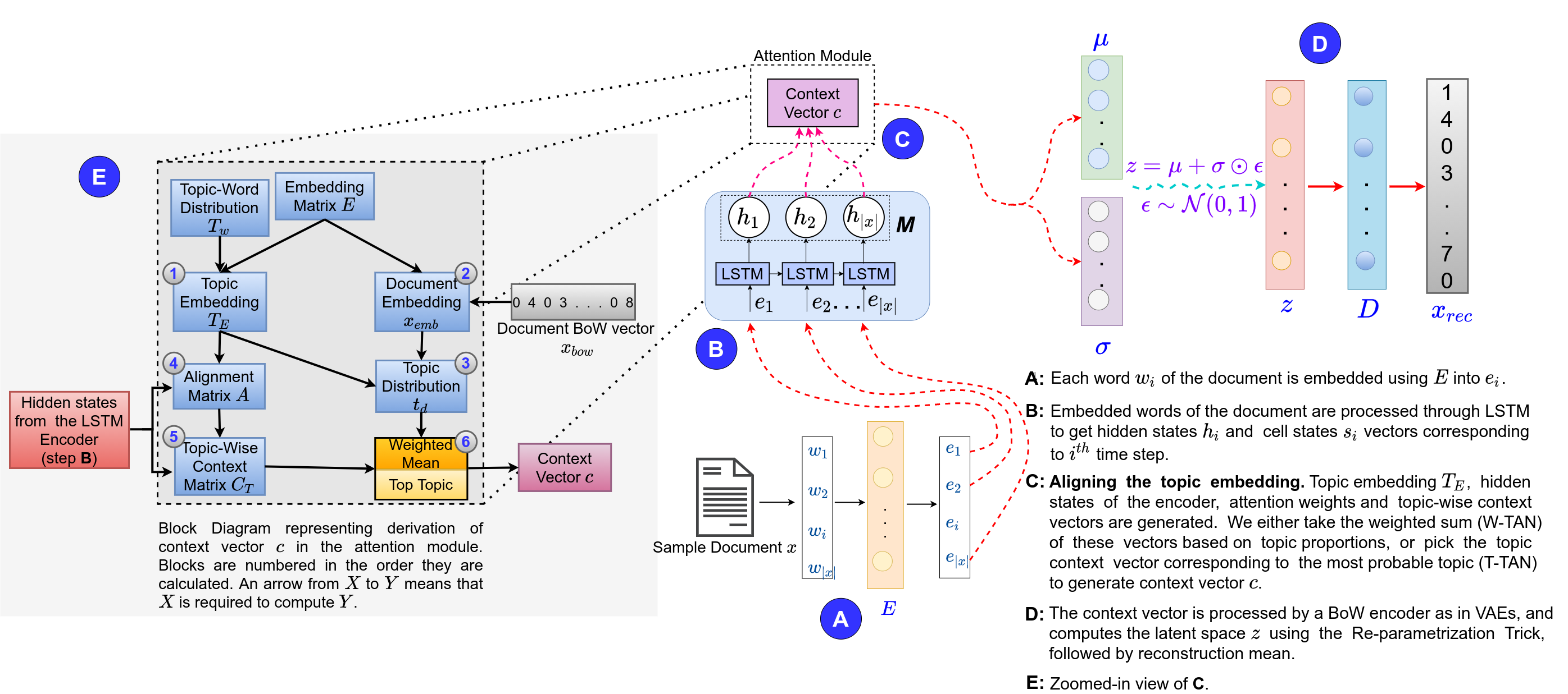
Figure 1: A-E: Architecture of TAN-NTM showing flow of document processing through it. Document, being embedded using embedding layer, is processed by LSTM, yielding hidden states on which TAN attends in a topic aware manner. The resultant context vector is used to perform variational inference and processed through a BoW decoder as in VAEs. Attention Module E (zoomed in view of C) computes the blocks in the mentioned order 1-6.

3 Background

LDA is a generative statistical model and assumes that each document is a distribution over a fixed number of topics (say $K$) and that each topic is a distribution of words over the entire vocabulary. LDA proposes an iterative process of document generation where for each document $d$, we draw a topic distribution $\theta$ from $Dirichlet(\alpha)$ distribution. For each word in $d$ at index $i$, we sample a topic $\mathbf{t}_{i}$ from $Multinomial(\theta)$ distribution. $\mathbf{w}_{i}$ is sampled from $p(\mathbf{w}_{i}|\mathbf{t}_{i},\beta)$ distribution which is a multinomial probability conditioned on topic $\mathbf{t}_{i}$. Given the document corpus and the parameters $\alpha$ and $\beta$, we need the joint probability distribution of a topic mixture $\theta$, a set of $K$ topics t, and a set of $n$ words w. This is given analytically by an intractable integral. The solution is to use Variational Inference wherein this problem is converted into an optimization problem for finding various parameters that minimize the KL divergence between the prior and the posterior distribution.

This idea is leveraged at scale by the use of Variational Autoencoders. The encoder processes BoW vector of the document $\mathbf{x}_{bow}$ by an MLP (Multi Layer Perceptron) which then forks into two independently trainable layers to yield $\mathbf{z}_{\mu}$ & $\mathbf{z}_{\log\sigma^{2}}$. Then a re-parametrization trick is employed to sample the latent vector $\mathbf{z}$ from a logistic-normal distribution (resulting from an approximation of Dirichlet distribution). This is essential since back-propagation through a sampling node is infeasible. $\mathbf{z}$ is then used by decoder’s single dense layer D to yield the reconstructed BoW $\mathbf{x}_{rec}$. The objective function has two terms: (a) Kullback–Leibler (KL) Divergence Term - to match the variational posterior over latent variables with the prior and (b) Reconstruction Term - categorical cross entropy loss between $\mathbf{x}_{bow}$ & $\mathbf{x}_{rec}$.

$$L_{NTM}=D_{KL}(p(\mathbf{z})\ ||\ q(\mathbf{z}|\mathbf{x}))-\mathbb{E}_{q(\mathbf{z}|\mathbf{x})}[p(\mathbf{x}|\mathbf{z})]$$

Our methodology improves upon the document encoder and introduces a topic guided attention whose output is used to sample $\mathbf{z}$. We use the same formulation of decoder as used in ProdLDA.

4 Methodology

In this section, we describe the details of our framework where we leverage the topic-word distribution to perform topic guided attention over tokens in a document. Given a collection $\mathcal{C}$ with $|C|$ documents $\mathbf{\{x_{1},x_{2},..,x_{|C|}\}}$, we process each document $\mathbf{x}$ into BoW vector $\mathbf{x}_{bow}\in\mathbb{R}^{|V|}$ and as a token sequence $\mathbf{x}_{seq}$, where V represents the vocabulary. As shown in step A in figure 1, each word $w_{j}\in\mathbf{x}_{seq}$ is embedded as $\mathbf{e}_{j}\in\mathbb{R}^{E}$ through an embedding layer $\mathbf{E}\in\mathbb{R}^{|V|\times E}$ ($E=$ Embedding Dimension) initialised with GloVe Pennington et al. (2014). The embedded sequence $\{{e}_{j}\}_{j=1}^{\mathbf{|x|}}$, where $\mathbf{|x|}$ is the number of tokens in $\mathbf{x}$, is processed through a sequence encoder LSTM Hochreiter and Schmidhuber (1997) to obtain the corresponding hidden states $\mathbf{h}_{j}\in\mathbb{R}^{H}$ and cell states $\mathbf{s}_{j}\in\mathbb{R}^{H}$ (step B in figure 1):

$$\mathbf{h}_{j},\mathbf{s}_{j}=f_{LSTM}(\mathbf{e}_{j},(\mathbf{h}_{j-1},\mathbf{s}_{j-1}))$$

where $H$ is LSTM’s hidden size. We construct a memory bank $\mathbf{M}=\langle\mathbf{h}_{1},\mathbf{h}_{2},...,\mathbf{h_{|x|}}\rangle$ which is then used to perform topic-guided attention (step C in figure 1). The output vector of the attention module is used to derive prior distribution parameters $\mathbf{z}_{\mu}$ & $\mathbf{z}_{\log\sigma^{2}}$ (as in VAE) through two linear layers. Using the re-parameterisation trick, we sample the latent document-topic vector $\mathbf{z}$, which is then given as input to BoW decoder linear layer $\mathbf{D}$ that outputs the reconstructed BoW $\mathbf{x}_{rec}$ (step D in figure 1). Objective function is same as in VAE setting, involving a reconstruction loss term between $\mathbf{x}_{rec}$ & $\mathbf{x}_{bow}$ and KL divergence between the prior (laplace approximation to Dirichlet prior as in ProdLDA) and posterior. We now discuss the details of our Topic Attention Network.

4.1 TAN: Topic Attention Network

We intend the model to attend on document words in a manner such that the resultant attention is distributed according to the semantics of the topics relevant to the document. We hypothesize that this can enable the model to encode better document features while capturing the underlying latent document-topic representations. The topic-word distribution $\mathbf{T_{w}}$ represents the affinity of each topic towards words in the vocabulary (which is used to interpret the semantics of each topic). Therefore, we factor $\mathbf{T_{w}}\in\mathbb{R}^{K\times|V|}$ into the attention mechanism, where K denotes the number of topics. The topic-aware attention encoder and topic-word distribution influence each other during training which consequently results in convergence to better topics as discussed in detail in Experiments section.

Specifically, we perform attention on document sequence of tokens for each topic using the embedded representation of the topics $\mathbf{T_{E}}\in\mathbb{R}^{K\times E}$:

$$\mathbf{T_{E}}=\mathbf{T_{w}}\mathbf{E},\ \ \ \ \textrm{[topic embeddings]}$$

$$\mathbf{T_{w}}=\mathrm{softmax}(\mathbf{D}),\ \ \ \ \textrm{[topic-word distribution]}$$

where $\mathbf{D}\in\mathbb{R}^{K\times V}$ is the decoder layer which is used to reconstruct $\mathbf{x}_{bow}$ from the sampled latent document-topic representation $\mathbf{z}$ as the final step D in Figure 1. The topic embeddings are then used to determine the attention alignment matrix $\mathbf{A}\in\mathbb{R}^{\mathbf{|x|}\times K}$ between each topic $k\in\{1,2,...,K\}$ and words in the document such that:

$$\mathbf{A}_{jk}=\frac{\mathrm{exp}(score((\mathbf{T_{E}})_{k},\mathbf{h}_{j}))}{\sum_{j^{\prime}=1}^{\mathbf{|x|}}\mathrm{exp}(score((\mathbf{T_{E}})_{k},\mathbf{h}_{j^{\prime}}))},$$

$$score((\mathbf{T_{E}})_{k},\mathbf{h}_{j})=\mathbf{v_{A}}^{\top}\mathrm{tanh}(\mathbf{W_{A}}[(\mathbf{T_{E}})_{k}\mathbf{;}\mathbf{h}_{j}])$$

where $\mathbf{v_{A}}\in\mathbb{R}^{P}$, $\mathbf{W_{A}}\in\mathbb{R}^{P\times(E+H)}$, $(\mathbf{T_{E}})_{k}\in\mathbb{R}^{E}$ is the embedded representation of the $k^{th}$ topic and ; is the concatenation operation. We then determine topic-wise context vector corresponding to each topic as:

$$\mathbf{C_{T}}=\sum_{j=1}^{\mathbf{|x|}}\mathbf{A}_{j}\otimes\mathbf{h}_{j},\ \ \ \ \textrm{[topic-wise context matrix]}$$

where $\otimes$ denotes outer product. Note that $\mathbf{A}_{j}$ $\in\mathbb{R}^{K}$ ($j^{th}$ row of matrix $\mathbf{A}$) is a $K$ - dimensional vector and $\mathbf{h}_{j}$ is a $H$ - dimensional vector, therefore $\mathbf{A}_{j}\otimes\mathbf{h}_{j}$ for each $j$ yields a matrix of order $K\times H$, hence $\mathbf{C_{T}}\in\mathbb{R}^{K\times H}$. The final aggregated context vector $\mathbf{c}$ is computed as a weighted average over all rows of $\mathbf{C_{T}}$ (each row representing each topic specific context vector) with document-topic proportion vector $\mathbf{t_{d}}$ as weights:

$$\mathbf{c}=\sum_{k=1}^{K}(\mathbf{t_{d}})_{i}(\mathbf{C_{T}})_{k}$$

where, $(\mathbf{t_{d}})_{k}$ is a scalar, $(\mathbf{C_{T}})_{k}\in\mathbb{R}^{H}$ denotes the $k^{th}$ row of matrix $\mathbf{C_{T}}$ & $\mathbf{t_{d}}$ is the document-topic distribution which signifies the topic proportions in a document. To compute it, we first normalize the document BoW vector $\mathbf{x}_{bow}$ and embed it using the embedding matrix $\mathbf{E}$, followed by multiplication with topic embedding $\mathbf{T_{E}}\in\mathbb{R}^{K\times E}$:

$$\mathbf{x}_{norm}=\frac{\mathbf{x}_{bow}}{\sum_{i=1}^{|V|}(\mathbf{x}_{bow})_{i}},\ \ \textrm{[normalized BoW]}$$

$$\mathbf{x}_{emb}=\mathbf{x}_{norm}^{\top}E,\ \ \ \ \ \ \ \ \ \ \textrm{[document embedding]}$$

$$\mathbf{t_{d}}=\mathrm{softmax}(\mathbf{T_{E}}\ \mathbf{x}_{emb}),\textrm{[document-topic dist.]}$$

where $\mathbf{x_{norm}}\in\mathbb{R}^{|V|}$, $\mathbf{x_{emb}}\in\mathbb{R}^{E}$ & $\mathbf{t_{d}}\in\mathbb{R}^{K}$. The context vector $\mathbf{c}$ is the output of our topic guided attention module which is then used for sampling the latent documents-topic vector followed by the BoW decoding as done in traditional VAE based topic models.

We call this framework as Weighted-TAN or W-TAN where the context vector $\mathbf{c}$ is a weighted sum of topic-wise context vectors. We also propose another model called Top-TAN or T-TAN where we use context vector of the topic with largest proportion in $\mathbf{t_{d}}$ as $\mathbf{c}$. It has been experimentally observed that doing so yields a model which generates more coherent topics. First, we find the index $m$ of most probable topic in $\mathbf{t_{d}}$. The context vector $\mathbf{c}$ is then the row corresponding to index $m$ in matrix $\mathbf{C_{T}}$.

5 Experiments

5.1 Datasets

1. Topic Quality: We evaluate and compare quality of our proposed topic model on three benchmark datasets - 20Newsgroups (20NG) Lang (1995), AGNews Zhang et al. (2015) and Yelp Review Polarity (YRP) - which are of varying complexity and scale in terms of number of documents, vocabulary size and average length of text after preprocessing. Table 1 summarises statistics related to these datasets used for evaluating topics quality.

Dataset	# Train	# Test	vocab	avg.doc.len.
20NG	11259	7488	1995	88.06
AGNews	96000	7600	27881	22.72
YRP	447873	38000	20001	54.46

Table 1: Datasets used for evaluating topic quality

2. Keyphrase Generation: Neural Topic Model (NTM) has been used to improve the task of supervised keyphrase generation Wang et al. (2019b). To further highlight the efficacy of our proposed encoding framework in providing better document-topic vectors, we modify encoder module of NTM with our proposed TAN-NTM and compare the performance on StackExchange and Weibo Datasets.

5.2 Implementation and Training Details

Documents in AGNews are padded upto a maximum length of $50$, while those in 20NG and YRP are padded upto $200$ tokens. Documents with longer lengths are truncated. These values were chosen such that $\sim 80-99\%$ of all documents in each dataset were included without truncation. We use batch size of 100, Adam Optimizer Kingma and Ba (2015) with $\beta_{1}=0.99$, $\beta_{2}=0.999$ and $\epsilon=10^{-8}$ and train each model for $200$ epochs. For all models except T-TAN, learning rate was fixed at $\textbf{0.002}\ ([0.001,\ 0.003],\ 5)$. T-TAN converges relatively faster than other models, therefore for smooth training, we decay its learning rate every epoch using exponential staircase scheduler with initial learning rate = 0.002 and decay rate = 0.96. The number of topics $K$ = $50$, a value widely used in literature. We perform hyper-parameter tuning manually to determine the hidden dimension value of various layers: $E$ = $\textbf{200}\ ([100,\ 300],\ 5)$, $H$ = $\textbf{450}\ ([300,\ 900],\ 10)$ and $P$ = $\textbf{350}\ ([10,\ 400],\ 10)$. The weight matrices of all dense layers are Xavier initialized, while bias terms are initialized with zeros. All our proposed models and baselines are trained on a machine with 32 virtual CPUs, single NVIDIA Tesla $V100$ GPU and 240 GB RAM.

5.3 Comparison with baselines

We compare our TAN-NTM with various baselines in table 2 that can be enumerated as (please refer to introduction and related work for their details):
1) LDA (C.G.): Statistical method McCallum (2002) which performs LDA using collapsed Gibbs sampling.
2) ProdLDA and 3) NVLDA Srivastava and Sutton (2017): Neural Variational Inference methods which use approximation to Dirichlet prior.
4) W-LDA Nan et al. (2019) which is a non variational inference based neural model using wassestein autoencoder.
5) NB-NTM and 6) GNB-NTM: Methods using negative binomial and gamma negative binomial distribution as priors for topic discoveryWu et al. (2020) respectively.

Method	20NG	AGNews	YRP
LDA(C.G)	0.139	0.202	0.114
NVLDA	0.2	0.216	0.165
ProdLDA	0.268	0.322	0.165
W-LDA	0.227	0.262	0.25
NB-NTM	0.165	0.31	0.224
GNB-NTM	0.206	0.312	0.241
W-TAN (ours)	0.261	0.327	0.232
T-TAN (ours)	0.296	0.369	0.272

Table 2: NPMI coherence (determined using top 10 words of each topic) comparison on 50 topics between baselines and our proposed W-TAN and T-TAN on different datasets. It can be seen that T-TAN achieves significantly better scores on all the datasets.

We could not compare with other methods whose official error-free source code is not publicly available yet. We train and evaluate the baseline methods on same data as used for our method using NPMI coherence Aletras and Stevenson (2013). It computes the semantic relatedness between top $L$ words in a given topic through determining similarity between their word embeddings trained over the corpus used for topic modeling and reports average over topics. For W-LDA, we refer to their original paper to select dataset specific hyper-parameter values while training the model. As can be seen in table 2, our proposed T-TAN model performs significantly better than previous topic models uniformly on all datasets achieving a better NPMI (measured on a scale of -1 to 1) by a margin of 0.028 (10.44%) on 20NG, 0.047 (14.59%) on AGNews and 0.022 (8.8%) on YRP, where percentage improvements are determined over the best baseline score. Even though W-TAN does not uniformly performs better than all baselines on all datasets, it achieves better score than all baselines on AGNews and performs comparably on remaining two datasets.

For a more exhaustive comparison, we also evaluate our model’s performance on 20NG dataset (which is the common dataset with GNB-NTM Wu et al. (2020)) using the NPMI metric from GNB-NTM’s code. The NPMI coherence of our model using their criteria is 0.395 which is better than GNB-NTM’s score of 0.375 (as reported in their paper). However, we would like to highlight that GNB-NTM’s computation of NPMI metric uses relaxed window size, whereas the metric used by us Lau et al. (2014) uses much stricter window size while determining word co-occurrence counts within a document. Lau et al. (2014) is a much more common and widely used way of computing the NPMI coherence and evaluating topic models.

5.3.1 Document Classification

In addition to evaluating our framework in terms of topic coherence, we also compare it with the baselines on the downstream task of document classification. Topic models have been used as text feature extractors to perform classification Nan et al. (2019). We analyse the quality of encoded document representations and predictive capacity of latent document-topic features generated by our model and compare it with existing topic models. We train the topic model setting number of topics to 50 and freeze its weights. The trained topic model is then used to infer latent document-topic features. We then separately train a single layer linear classifier through cross entropy loss on the training split using the document-topic vectors as input and Adam optimizer at a learning rate of 0.01.

Method	20NG	AGNews	YRP
LDA(C.G.)	51.29	84.78	86.85
ProdLDA	21.33	82.65	77.73
NTM-R	43.34	85.67	86.16
W-LDA	43.08	85.29	85.63
NB-NTM	57.38	86.67	87.51
GNB-NTM	57.16	85.34	84.55
T-TAN (ours)	60.44	88.1	87.38
T-TAN (ours)	64.36	89.78	88.9
(context vector)

Table 3: Comparison of accuracy between different topic models on document classification. We perform two experiments with T-TAN: using document-topic vector ($2^{nd}$ to last row) and context vector (last row).

We report classification accuracy on the test split of 20NG, AGNews and YRP datasets (comprising of 20, 4 and 2 classes respectively) in Table 3. The document-topic features provided by T-TAN achieve best accuracy on AGNews (1.43% improvement over most performant baseline) with most significant improvement of 3.06% on 20NG which shows our model learns better document features. T-TAN performs almost the same as the best baseline on YRP. Further, to analyse the predictive performance of top topic attention based context vector, we use it instead of latent document-topic vector to perform classification which further boosts accuracy leading to an improvement of $\sim$6.9% on 20NG, $\sim$3.1% on AGNews and $\sim$1.3% on YRP datasets over the baselines.

5.3.2 Running Time Analysis

We compare the running time of our method with baselines in terms of average time taken (in seconds) for performing a forward pass through the model, where the average is taken over 10000 passes. Our TAN-NTM (implemented in tensorflow) takes 0.087s, 0.027s and 0.093s on 20NG, AGNews and YRP datasets respectively. Since TAN-NTM processes the input documents as a sequence of tokens through an LSTM, its running time is proportional to the document lengths which vary according to the dataset. The running time for baseline methods are: ProdLDA - 0.012s (implemented in tensorflow), W-LDA - 0.003s (implemented in mxnet) and GNB-NTM - 0.003s (implemented in pytorch). For baseline methods, we have used their original code implementations. We found that the running time of baseline models is independent of the dataset. This is because they use the Bag-of-Words (BoW) representation of the documents. The sequential processing in TAN-NTM is the reason for increased running time of our models compared to the baselines. In the case of AGNews, since the documents are of lesser lengths than 20NG and YRP, the running time of our TAN-NTM is relatively less for AGNews. Further, the running time of other ablation variants (introduced in section 5.4) of our method on 20NG, AGNews and YRP datasets respectively are: 1) only LSTM - 0.083s, 0.033s and 0.091s ; 2) vanilla attn - 0.088s, 0.037s and 0.095s.

5.4 Ablation Studies

In this section, we compare the performance of different variants of our model namely, 1) only LSTM: final hidden state is used to derive sampling parameters $\mathbf{z}_{\mu}$ & $\mathbf{z}_{\log\sigma^{2}}$, 2) vanilla attn: final hidden state (w/o topic-word distribution) is used as query to perform attention Bahdanau et al. (2014) on LSTM outputs such that context vector $\mathbf{z}$ is used for VI, 3) W-TAN: Weighted Topic Attention Network, 4) T-TAN: Top Topic Attention Network and 5) T-TAN w/o (without) GloVe: embedding layer in T-TAN is randomly initialised.

Table 4 compares the topic coherence scores of these different ablation methods on 20NG, AGNews and YRP. As can be seen, applying attention performs better than simple LSTM model. The weighted TAN performs better than vanilla attention model, however, T-TAN uniformly provides the best coherence scores across all the datasets compared to all other methods. This shows that performing attention corresponding to the most prominent topic in a document results in more coherent topics. Further, we perform an ablation to study the effect of using pre-trained embeddings for T-TAN where it can be seen using Glove for initialising word embeddings results in improved NPMI as compared to training T-TAN initialised with random uniform embeddings (T-TAN w/o GloVe).

Method	20NG	AGNews	YRP
only LSTM	0.247	0.202	0.092
vanilla attn	0.289	0.244	0.18
W-TAN	0.261	0.327	0.232
T-TAN	0.296	0.369	0.272
T-TAN w/o GloVe	0.274	0.344	0.248

Table 4: Comparison of NPMI coherence between ablation variants of our method for K=50 topics.

	StackExchange			Weibo
Method	F1@3	F1@5	MAP	F1@1	F1@3	MAP
TAKG (baseline)	32.931	28.731	34.925	34.584	24.309	40.994
TAKG with W-TAN (ours)	33.521	29.802	35.929	35.616	25.651	42.68
TAKG with T-TAN (ours)	33.15	29.118	35.26	34.813	24.65	41.261

Table 5: F1@k and MAP (Mean average precision) comparison between baseline (TAKG) and our proposed topic model based encoder for topic guided supervised keyphrase generation. The metrics measure overlap between ground truth and top K generated keyphrases factoring in rank of keyphrases generated through beam search.

5.5 Qualitative Analysis

To verify performance of T-TAN qualitatively, we display few topics generated by ProdLDA and T-TAN on AGNews in Figure 2. ProdLDA achieves best score among baselines on AGNews. Consider comparison 1 in Figure 2: ProdLDA produces four topics corresponding to space, mixing them with nuclear weapons, while T-TAN produces two separate topics for both of these concepts. In second comparison, we see that ProdLDA has problems distinguishing between closely related topics (football, olympics, cricket) and mixes them while T-TAN produces three coherent topics.

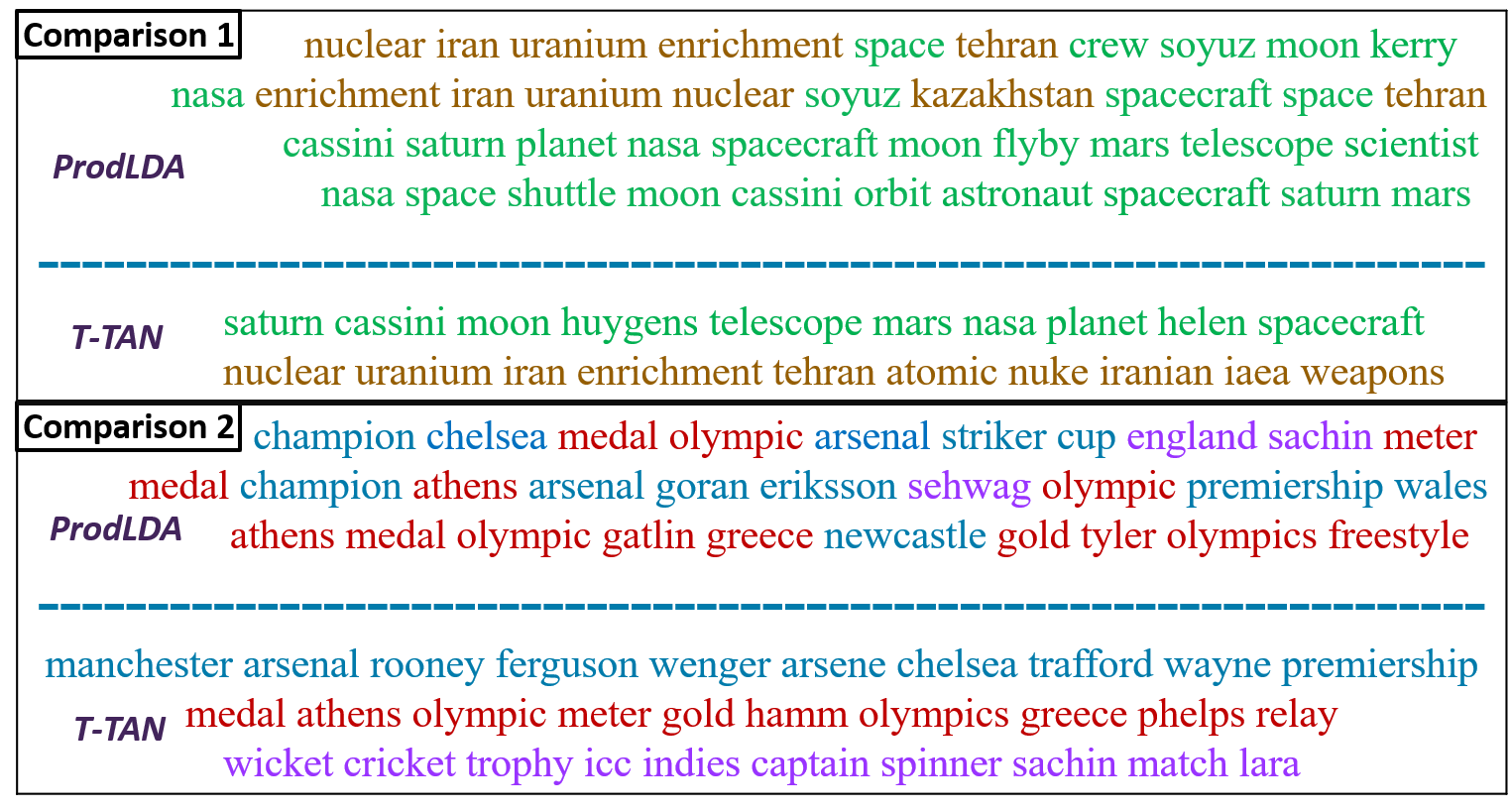
Figure 2: Two comparisons of corresponding topics (one topic per line) from ProdLDA and T-TAN. Words having similar meaning are highlighted in same colour. The topics of ProdLDA are inter-mixed and incoherent while those of T-TAN are unmixed and coherent.

5.6 TAKG: Topic Aware Keyphrase Generation

We further analyse the impact of our proposed framework on another downstream task where the task specific model is assisted by the topic model and both can be trained in an end-to-end manner. For this, we discuss TAKG Wang et al. (2019b) and how our proposed topic model encoder can be adapted to achieve better performance on supervised keyphrase generation from textual posts. TAKG comprises of two sub-modules: (1) a topic model based on NVDM-GSM (as discussed in Introduction) using BoW as input to the encoder and (2) a Seq2Seq based model for keyphrase generation. Both modules have an encoder and a decoder of their own. Keyphrase generation module uses sequence input which is processed by bidirectional GRU Cho et al. (2014) to encode input sequence. The keyphrase generation decoder uses unidirectional GRU which attends on encoder outputs and takes the latent document-topic vector from the topic model as input in a differentiable manner. Since topic model trains slower than keyphrase generation module, the topic model is warmed up for some epochs separately and then jointly trained with keyphrase generation. Please refer to original paper Wang et al. (2019b) for more details.

We adapted our proposed topic model framework by changing the architecture of encoder in the topic model of TAKG, replacing it with W-TAN and T-TAN. The change subsequently results in better latent document-topic representation depicted by better performance on keyphrase generation as shown in Table 5 where the improved topic model encoding framework results in $\sim$1-2% improvement in F1 and MAP (mean average precision) on StackExchange and Weibo datasets compared to TAKG. Here, even though TAKG with T-TAN performs marginally better than the baseline, TAKG with W-TAN uniformly performs much better.

6 Conclusion

In this work, we propose Topic Attention Network based Neural Topic Modeling framework: TAN-NTM to discover topics in a document corpus by performing attention on sequentially processed tokens in a topic guided manner. Attention is performed effectively by factoring Topic-word distribution (TWD) into attention mechanism. We compare different variants of our method through ablations and conclude that processing tokens sequentially without attention or applying attention without TWD gives inferior performance. Our TAN-NTM model generates more coherent topics compared to state-of-the-art topic models on several benchmark datasets. Our model encodes better latent document-topic features as validated through better performance on document classification and supervised keyphrase generation tasks. As future work, we would like to explore our framework with other sequence encoders such as Transformers, BERT etc. for topic modeling.

Appendices

Appendix A Further Implementation Details

A.1 Preprocessing

For 20NG dataset, we used its preprocessed version downloaded from ProdLDA’s Srivastava and Sutton (2017) repository, whereas AGNews and YRP datasets were downloaded from this link. These two datasets contain train.csv and test.csv files. The csv files of YRP contain a document body only, whereas the csv files for AGNews contain a document title as well as a document body. For uniformity, we concatenate the title and body in the csv files of AGNews and keep it as a single field. The documents from train.csv and test.csv are then read into train and test lists which are passed to preprocess function of Algorithm 1 for preprocessing.

Stepwise working of Algorithm 1 is expained in the following points:

• Before invoking the preprocess function, we initialize the data sampler by a fixed seed so that preprocessing yields the same result when run multiple times.

• For each dataset, we randomly sample tr_size documents (as mentioned in Table 6) from the train list in step 2. These values of tr_size are taken from Table 1 of W-LDA paper Nan et al. (2019). Note that # Train in Table 1 represents the number of training documents after preprocessing. Of the tr_size documents, some documents may be removed during preprocessing, therefore # Train may be less than tr_size.

• In steps 3 through 8, we prune the train and test documents by invoking the prune_doc function from Algorithm 2. First, we remove the control characters from the documents viz. ‘\n’, ‘\t’, and ‘\r’ (For YRP, we additionally remove ‘\\t’, ‘\\n’, and ‘\\r’). Next, we remove the numeric tokens from the documents, convert them to lowercase and lemmatize each of their tokens using the NLTK’s Bird et al. (2009) WordNetLemmatizer. Finally, we remove punctuations and tokens containing any non-ASCII character.

• In steps 9 through 15, we construct the vocabulary vocab, which is a mapping of each token to its occurrence count among the pruned training documents tr_pruned. We only count a token if it is not an English stopword and its length is between 3 and 15 (inclusive).

• Steps 16 through 19 filter the vocab by removing tokens whose total occurrence count is less than num_below or whose occurrence count per training document is greater than fr_abv, where the values of num_below and fr_abv are taken from Table 6. For YRP, we follow the W-LDA paper Nan et al. (2019) and restrict its vocab to only contain top $20,000$ most occurring tokens.

• Steps 20 through 24 construct the token-to-index map w2idx by mapping each token in vocab to an index starting from 1. Next, we map the padding token to index $0$ (Step 25).

• The final step in the preprocessing is to encode the train and test documents by mapping each of their tokens to corresponding indices according to w2idx. This is done by the encode function of Algorithm 2 which is invoked in steps 26 and 27.

Dataset	tr_size	num_below	fr_abv
AGNews	96000	3	0.7
YRP	448000	20	0.7

Table 6: Parameters used for preprocessing the AGNews and YRP datasets.

Algorithm 1 Pseudocode for preprocessing AGNews and YRP datasets.

1:function preprocess(train, test)

2:     train $\leftarrow$ train.$sample$(tr_size)

3:     tr_pruned $\leftarrow$ [] $\triangleright$ empty list

4:     te_pruned $\leftarrow$ [] $\triangleright$ empty list

5:

6:     for document $d$ in train do

7:         tr_pruned.$append$(prune_doc($d$))      

8:

9:     for document $d$ in test do

10:         te_pruned.$append$(prune_doc($d$))      

11:

12:     vocab $\leftarrow$ mapping of each token to $0$

13:     num_doc $\leftarrow$ $len$(tr_pruned)

14:

15:     for document $d$ in tr_pruned do

16:         for token $t$ in $d$ do

17:              if $t\notin stopwords$ and

18:              $len(t)\in[3,15]$ then

19:                  vocab[$t$]$\leftarrow$ vocab[$t$] $+1$                             

20:     for token $t$ in vocab do

21:         if vocab[$t$] $<$ num_below or

22:         vocab[$t$]$/$num_doc $>$ fr_abv then

23:              vocab[$t$]$.remove(t)$               

24:

25:     $i$ $\leftarrow$ 1

26:     w2idx $\leftarrow$ empty map

27:     for token $t$ in vocab do

28:         w2idx[$t$]$=i$

29:         $i\leftarrow i+1$      

30:     w2idx[$0$]$\leftarrow\mathbb{PAD}$

31:

32:     trD $\leftarrow$ encode(tr_pruned, w2idx)

33:     teD $\leftarrow$ encode(te_pruned, w2idx)

34:     return trD, teD, w2idx

35:

A.2 Learning Rate Scheduler

As mentioned in section 5.2, we use a learning rate scheduler while training T-TAN. The rate decay follows the following equation:

$$lrate=init\_rate*decay\_rate^{\left\lfloor{\frac{train\_step}{decay\_steps}}\right\rfloor}$$

This is an exponential staircase function which enables decrease in learning rate every epoch during training.

Algorithm 2 Pseudocode for pruning the document and encoding it given a token-to-index mapping.

1:function prune_doc(doc)

2:     doc $\leftarrow$ $rm\_control$(doc)

3:     doc $\leftarrow$ $rm\_numeric$(doc)

4:     doc $\leftarrow$ $lowercase$(doc)

5:     doc $\leftarrow$ $lemmatize$(doc)

6:     doc $\leftarrow$ $rm\_punctuations$(doc)

7:     doc $\leftarrow$ $rm\_non\_ASCII$(doc)

8:     return doc

9:

10:function encode(doc_list, w2idx)

11:     encDocList $\leftarrow$ []

12:     for document $d$ in doc_list do

13:         ecDoc $\leftarrow$ []

14:         for token $t$ in $d$ do

15:              ecDoc$.append$(w2idx[$t$])          

16:         encDocList$.append$(ecDoc)      

17:     return encDocList

We initialize the learning rate by $init\_rate=0.002$ and use $decay\_rate=0.96.$ $train\_step$ is a global counter of training steps and $decay\_steps=\frac{\#train\_docs}{batch\_size}$ is the number of training steps taken per epoch. Therefore, effectively, the rate remains constant for all training steps in an epoch and decreases exponentially as per the above equation once the epoch completes.

A.3 Regularization

We employ two types of regularization during training:

• Dropout: We apply dropout Srivastava et al. (2014) to $z$ with the rate of $P_{drop}=0.6$ before it is processed by the decoder for reconstruction.

• Batch Normalization (BN): We apply a BN Ioffe and Szegedy (2015) to the inputs of decoder layer and to the inputs of layers being trained for $z_{\mu}$ & $z_{\log\sigma^{2}}$, with $\epsilon=0.001$ and $decay=0.999$.

Appendix B Evaluation Metrics

Topic models have been evaluated using various metrics namely perplexity, topic coherence, topic uniqueness etc. However, due to the absence of a gold standard for the unsupervised task of topic modeling, all of that metrics have received criticism by the community. Therefore, a consensus on the best metric has not been reached so far. Perplexity has been found to be negatively correlated to topic quality and human judgements Chang et al. (2009). This work presents experimental results which show that in some cases models with higher perplexity were preferred by human subjects.

Topic Uniqueness Nan et al. (2019) quantifies the intersection among topic words globally. However, it also suffers from drawbacks and often penalizes a model incorrectly Hoyle et al. (2020b). Firstly, it does not account for ranking of intersected words in the topics. Secondly, it fails to distinguish between the following two scenarios: 1) When the intersected words in one topic are all present in a second topic (signifying strong similarity i.e. these two topics are essentially identical) and, 2) When the intersected words of one topic are spread across all the other topics (signifying weak similarity i.e. the topics are diffused). The first is a problem related to uniqueness among topics while second is a problem related to word intrusion in topics. Chang et al. (2009) conducted experiments with human subjects on two tasks: word intrusion and topic intrusion. Word intrusion measures the presence of those words (called intruder words) which disagree with the semantics of the topic. Topic intrusion measures the presence of those topics (called intruder topics) which do not represent the document corpus appropriately. These are better estimates of human judgement of topic models in comparison to perplexity and uniqueness. However, since these metrics rely on human feedback, they cannot be widely used for unsupervised evaluation. Further, topic uniqueness unfairly penalizes cases when some words are common between topics, however other uncommon words in those topics change the context as well as topic semantics as also discussed in Hoyle et al. (2020b). According to the work of Lau et al. (2014), measuring the normalized pointwise mutual information (NPMI) between all the word pairs in a set of topics agrees with human judgements most closely. This is called the NPMI Topic Coherence in the literature and is widely used for the evaluation of topic models. We therefore adopt this metric in our work. Since the effectiveness of a topic model actually depends on the topic representations that it extracts from the documents, we report the performance of our model on two downstream tasks: document classification and keyphrase generation (which use these topic representations) for a better and holistic evaluation and comparison.

Would a pilot know that one of their crew is armed?

The Federal Flight Deck Officer page on Wikipedia says this:

Under the FFDO program, flight crew members are authorized to use firearms. A flight crew member may be a pilot, flight engineer or navigator assigned to the flight.

To me, it seems like this would be crucial information for the PIC to know, if their flight engineer (for example) was armed; but on the flip-side of this, the engineer might want to keep that to himself if he’s with a crew he hasn’t flown with before.

Is there a guideline on whether an FFDO should inform the crew that he’s armed?

GT: security, crew, ffdo

TAKG: faa regulations, ffdo, flight training, firearms, far

TAKG + W-TAN: ffdo, crew, flight controls, crewed spaceflight, security

Do the poisons in “Ode on Melancholy” have deeper meaning?

In ”Ode on Melancholy”, Keats uses the images of three poisons in the first stanza: Wolf’s bane, nightshade, and yew-berries. Are these poisons simply meant to connote death/suicide, or might they have a deeper purpose?

GT: poetry, meaning, john keats

TAKG: the keats, meaning, poetry, ode, melancholy keats

TAKG + W-TAN: poetry, meaning, the keats, john keats, greek literature

Table 7: Two randomly selected posts (title in bold) from StackExchange dataset with ground truth (GT) and top 5 keyphrases predicted by TAKG with and without W-TAN, denoted as TAKG + W-TAN & TAKG respectively. Keyphrases generated with W-TAN are closer to the ground truth in terms of both prediction and ranking.

Appendix C Qualitative Analysis

C.1 Key Phrase Predictions

We saw the quantitative improvement in results in Table 5 when we used W-TAN as the topic model with TAKG. In Table 7, we display some posts from StackExchange dataset with ground truth keyphrases and top 5 predictions by TAKG with and without W-TAN. We observe that using W-TAN improves keyphrase generation qualitatively.

The first post in Table 7 inquires if a flight officer should inform the pilot in command (PIC) about him being armed or not. For this post, TAKG alone only predicts one ground truth keyphrase correctly and misses ‘security’ and ‘crew’. However, when TAKG is used with W-TAN, it gets all three ground truth keyphrases, two of which are its top 2 predictions as well.

The second post is inquiring about a possible deeper meaning of three poisons in a poem by John Keats. TAKG alone predicts two of the ground truth keyphrases correctly but assigns them larger ranks and it misses ‘john keats’. When TAKG is used with W-TAN, it gets all three ground truth keyphrases and its top 2 keyphrases are assigned the exact same rank as they have in the ground truth. This hints that using W-TAN with TAKG improves the prediction as well as ranking of the generated keyphrases compared to using TAKG alone.

References

- Aletras and Stevenson (2013) Nikolaos Aletras and Mark Stevenson. 2013. Evaluating topic coherence using distributional semantics. In Proceedings of the 10th International Conference on Computational Semantics (IWCS 2013)–Long Papers, pages 13–22.
- Andrieu et al. (2003) Christophe Andrieu, Nando De Freitas, Arnaud Doucet, and Michael I Jordan. 2003. An introduction to mcmc for machine learning. Machine learning, 50(1-2):5–43.
- Bahdanau et al. (2014) Dzmitry Bahdanau, Kyunghyun Cho, and Yoshua Bengio. 2014. Neural machine translation by jointly learning to align and translate. arXiv preprint arXiv:1409.0473.
- Bianchi et al. (2020) Federico Bianchi, Silvia Terragni, and Dirk Hovy. 2020. Pre-training is a hot topic: Contextualized document embeddings improve topic coherence. ArXiv, abs/2004.03974.
- Bird et al. (2009) Steven Bird, Ewan Klein, and Edward Loper. 2009. Natural Language Processing with Python. O’Reilly Media.
- Blei et al. (2003) David M Blei, Andrew Y Ng, and Michael I Jordan. 2003. Latent dirichlet allocation. Journal of machine Learning research, 3(Jan):993–1022.
- Burkhardt and Kramer (2019) S. Burkhardt and S. Kramer. 2019. Decoupling sparsity and smoothness in the dirichlet variational autoencoder topic model. J. Mach. Learn. Res., 20:131:1–131:27.
- Card et al. (2018) Dallas Card, Chenhao Tan, and Noah A. Smith. 2018. Neural models for documents with metadata. In Proceedings of the 56th Annual Meeting of the Association for Computational Linguistics (Volume 1: Long Papers), pages 2031–2040, Melbourne, Australia. Association for Computational Linguistics.
- Chang et al. (2009) Jonathan Chang, Sean Gerrish, Chong Wang, Jordan Boyd-graber, and David Blei. 2009. Reading tea leaves: How humans interpret topic models. In Advances in Neural Information Processing Systems, volume 22, pages 288–296. Curran Associates, Inc.
- Chen et al. (2018) Jun Chen, Xiaoming Zhang, Yu Wu, Zhao Yan, and Zhoujun Li. 2018. Keyphrase generation with correlation constraints. In Proceedings of the 2018 Conference on Empirical Methods in Natural Language Processing, pages 4057–4066, Brussels, Belgium. Association for Computational Linguistics.
- Cho et al. (2014) Kyunghyun Cho, Bart van Merriënboer, Caglar Gulcehre, Dzmitry Bahdanau, Fethi Bougares, Holger Schwenk, and Yoshua Bengio. 2014. Learning phrase representations using RNN encoder–decoder for statistical machine translation. In Proceedings of the 2014 Conference on Empirical Methods in Natural Language Processing (EMNLP), pages 1724–1734, Doha, Qatar. Association for Computational Linguistics.
- Deerwester et al. (1990) Scott Deerwester, Susan T. Dumais, George W. Furnas, Thomas K. Landauer, and Richard Harshman. 1990. Indexing by latent semantic analysis. Journal of the American Society for Information Science, 41(6):391–407.
- Devlin et al. (2019) Jacob Devlin, Ming-Wei Chang, Kenton Lee, and Kristina Toutanova. 2019. BERT: Pre-training of deep bidirectional transformers for language understanding. In Proceedings of the 2019 Conference of the North American Chapter of the Association for Computational Linguistics: Human Language Technologies, Volume 1 (Long and Short Papers), pages 4171–4186, Minneapolis, Minnesota. Association for Computational Linguistics.
- Dieng et al. (2020) Adji B. Dieng, Francisco J. R. Ruiz, and David M. Blei. 2020. Topic modeling in embedding spaces. Transactions of the Association for Computational Linguistics, 8:439–453.
- Dieng et al. (2016) Adji B Dieng, Chong Wang, Jianfeng Gao, and John Paisley. 2016. Topicrnn: A recurrent neural network with long-range semantic dependency. arXiv preprint arXiv:1611.01702.
- Ding et al. (2018) Ran Ding, Ramesh Nallapati, and Bing Xiang. 2018. Coherence-aware neural topic modeling. In Proceedings of the 2018 Conference on Empirical Methods in Natural Language Processing, pages 830–836, Brussels, Belgium. Association for Computational Linguistics.
- Goodfellow et al. (2014) Ian Goodfellow, Jean Pouget-Abadie, Mehdi Mirza, Bing Xu, David Warde-Farley, Sherjil Ozair, Aaron Courville, and Yoshua Bengio. 2014. Generative adversarial nets. In Z. Ghahramani, M. Welling, C. Cortes, N. D. Lawrence, and K. Q. Weinberger, editors, Advances in Neural Information Processing Systems 27, pages 2672–2680. Curran Associates, Inc.
- Griffiths and Steyvers (2004) Thomas L Griffiths and Mark Steyvers. 2004. Finding scientific topics. Proceedings of the National academy of Sciences, 101(suppl 1):5228–5235.
- Gupta et al. (2019) Pankaj Gupta, Yatin Chaudhary, Florian Buettner, and Hinrich Schütze. 2019. Document informed neural autoregressive topic models with distributional prior. In Proceedings of the AAAI Conference on Artificial Intelligence, volume 33, pages 6505–6512.
- Gururangan et al. (2019) Suchin Gururangan, T. Dang, D. Card, and Noah A. Smith. 2019. Variational pretraining for semi-supervised text classification. In ACL.
- Hochreiter and Schmidhuber (1997) Sepp Hochreiter and Jürgen Schmidhuber. 1997. Long short-term memory. Neural Comput., 9(8):1735–1780.
- Hoyle et al. (2020a) Alexander Miserlis Hoyle, Pranav Goel, and P. Resnik. 2020a. Improving neural topic models using knowledge distillation. ArXiv, abs/2010.02377.
- Hoyle et al. (2020b) Alexander Miserlis Hoyle, Pranav Goel, and Philip Resnik. 2020b. Improving Neural Topic Models using Knowledge Distillation. In Proceedings of the 2020 Conference on Empirical Methods in Natural Language Processing (EMNLP), pages 1752–1771, Online. Association for Computational Linguistics.
- Hu et al. (2020) Xuemeng Hu, Rui Wang, Deyu Zhou, and Yuxuan Xiong. 2020. Neural topic modeling with cycle-consistent adversarial training. In EMNLP.
- Ioffe and Szegedy (2015) S. Ioffe and Christian Szegedy. 2015. Batch normalization: Accelerating deep network training by reducing internal covariate shift. ArXiv, abs/1502.03167.
- Jin et al. (2018) Mingmin Jin, Xin Luo, Huiling Zhu, and Hankz Hankui Zhuo. 2018. Combining deep learning and topic modeling for review understanding in context-aware recommendation. In Proceedings of the 2018 Conference of the North American Chapter of the Association for Computational Linguistics: Human Language Technologies, Volume 1 (Long Papers), pages 1605–1614, New Orleans, Louisiana. Association for Computational Linguistics.
- Kingma and Ba (2015) Diederik P. Kingma and Jimmy Ba. 2015. Adam: A method for stochastic optimization. CoRR, abs/1412.6980.
- Kingma and Welling (2013) Diederik P Kingma and Max Welling. 2013. Auto-encoding variational bayes. arXiv preprint arXiv:1312.6114.
- Kumar et al. (2019) Varun Kumar, Alison Smith-Renner, Leah Findlater, K. Seppi, and Jordan L. Boyd-Graber. 2019. Why didn’t you listen to me? comparing user control of human-in-the-loop topic models. In ACL.
- Lang (1995) Ken Lang. 1995. Newsweeder: Learning to filter netnews. In Machine Learning Proceedings 1995, pages 331–339. Elsevier.
- Lau et al. (2014) Jey Han Lau, David Newman, and Timothy Baldwin. 2014. Machine reading tea leaves: Automatically evaluating topic coherence and topic model quality. In Proceedings of the 14th Conference of the European Chapter of the Association for Computational Linguistics, pages 530–539, Gothenburg, Sweden. Association for Computational Linguistics.
- McCallum (2002) Andrew Kachites McCallum. 2002. Mallet: A machine learning for language toolkit. http://mallet. cs. umass. edu.
- Meng et al. (2017) Rui Meng, Sanqiang Zhao, Shuguang Han, Daqing He, Peter Brusilovsky, and Yu Chi. 2017. Deep keyphrase generation. In Proceedings of the 55th Annual Meeting of the Association for Computational Linguistics (Volume 1: Long Papers), pages 582–592, Vancouver, Canada. Association for Computational Linguistics.
- Miao et al. (2017) Yishu Miao, Edward Grefenstette, and Phil Blunsom. 2017. Discovering discrete latent topics with neural variational inference. volume 70 of Proceedings of Machine Learning Research, pages 2410–2419, International Convention Centre, Sydney, Australia. PMLR.
- Miao et al. (2016) Yishu Miao, Lei Yu, and Phil Blunsom. 2016. Neural variational inference for text processing. volume 48 of Proceedings of Machine Learning Research, pages 1727–1736, New York, New York, USA. PMLR.
- Nan et al. (2019) Feng Nan, Ran Ding, Ramesh Nallapati, and Bing Xiang. 2019. Topic modeling with Wasserstein autoencoders. In Proceedings of the 57th Annual Meeting of the Association for Computational Linguistics, pages 6345–6381, Florence, Italy. Association for Computational Linguistics.
- Peinelt et al. (2020) Nicole Peinelt, Dong Nguyen, and Maria Liakata. 2020. tBERT: Topic models and BERT joining forces for semantic similarity detection. In Proceedings of the 58th Annual Meeting of the Association for Computational Linguistics, pages 7047–7055, Online. Association for Computational Linguistics.
- Pennington et al. (2014) Jeffrey Pennington, Richard Socher, and Christopher D Manning. 2014. Glove: Global vectors for word representation. In Proceedings of the 2014 conference on empirical methods in natural language processing (EMNLP), pages 1532–1543.
- Pergola et al. (2019) Gabriele Pergola, Lin Gui, and Yulan He. 2019. Tdam: a topic-dependent attention model for sentiment analysis. Inf. Process. Manag., 56.
- Řehůřek and Sojka (2010) Radim Řehůřek and Petr Sojka. 2010. Software Framework for Topic Modelling with Large Corpora. In Proceedings of the LREC 2010 Workshop on New Challenges for NLP Frameworks, pages 45–50, Valletta, Malta. ELRA.
- Rezaee and Ferraro (2020) Mehdi Rezaee and F. Ferraro. 2020. A discrete variational recurrent topic model without the reparametrization trick. ArXiv, abs/2010.12055.
- Sia et al. (2020) Suzanna Sia, Ayush Dalmia, and Sabrina J. Mielke. 2020. Tired of topic models? clusters of pretrained word embeddings make for fast and good topics too! In Proceedings of the 2020 Conference on Empirical Methods in Natural Language Processing (EMNLP), pages 1728–1736, Online. Association for Computational Linguistics.
- Srivastava and Sutton (2017) Akash Srivastava and Charles Sutton. 2017. Autoencoding variational inference for topic models. arXiv preprint arXiv:1703.01488.
- Srivastava et al. (2014) Nitish Srivastava, Geoffrey E. Hinton, A. Krizhevsky, Ilya Sutskever, and R. Salakhutdinov. 2014. Dropout: a simple way to prevent neural networks from overfitting. J. Mach. Learn. Res., 15:1929–1958.
- Steyvers and Griffiths (2007) Mark Steyvers and Tom Griffiths. 2007. Probabilistic topic models. Handbook of latent semantic analysis, 427(7):424–440.
- Thibaux and Jordan (2007) Romain Thibaux and Michael I. Jordan. 2007. Hierarchical beta processes and the indian buffet process. volume 2 of Proceedings of Machine Learning Research, pages 564–571, San Juan, Puerto Rico. PMLR.
- Tolstikhin et al. (2017) Ilya Tolstikhin, Olivier Bousquet, Sylvain Gelly, and Bernhard Schoelkopf. 2017. Wasserstein auto-encoders. arXiv preprint arXiv:1711.01558.
- Viegas et al. (2020) Felipe Viegas, Washington Cunha, Christian Gomes, Antônio Pereira, Leonardo Rocha, and Marcos Goncalves. 2020. CluHTM - semantic hierarchical topic modeling based on CluWords. In Proceedings of the 58th Annual Meeting of the Association for Computational Linguistics, pages 8138–8150, Online. Association for Computational Linguistics.
- Wang et al. (2020) Rui Wang, Xuemeng Hu, Deyu Zhou, Yulan He, Yuxuan Xiong, Chenchen Ye, and Haiyang Xu. 2020. Neural topic modeling with bidirectional adversarial training. In Proceedings of the 58th Annual Meeting of the Association for Computational Linguistics, pages 340–350, Online. Association for Computational Linguistics.
- Wang et al. (2019a) Rui Wang, Deyu Zhou, and Yulan He. 2019a. Atm: Adversarial-neural topic model. Information Processing & Management, 56(6):102098.
- Wang and Yang (2020) X. Wang and Y. Yang. 2020. Neural topic model with attention for supervised learning. In AISTATS.
- Wang et al. (2019b) Yue Wang, Jing Li, Hou Pong Chan, Irwin King, Michael R. Lyu, and Shuming Shi. 2019b. Topic-aware neural keyphrase generation for social media language. In Proceedings of the 57th Annual Meeting of the Association for Computational Linguistics, pages 2516–2526, Florence, Italy. Association for Computational Linguistics.
- Wu et al. (2020) Jiemin Wu, Yanghui Rao, Zusheng Zhang, Haoran Xie, Qing Li, Fu Lee Wang, and Ziye Chen. 2020. Neural mixed counting models for dispersed topic discovery. In Proceedings of the 58th Annual Meeting of the Association for Computational Linguistics, pages 6159–6169, Online. Association for Computational Linguistics.
- Zaheer et al. (2017) M. Zaheer, Amr Ahmed, and Alex Smola. 2017. Latent lstm allocation: Joint clustering and non-linear dynamic modeling of sequence data. In ICML.
- Zhang and Lauw (2020) Ce Zhang and Hady W. Lauw. 2020. Topic modeling on document networks with adjacent-encoder. In AAAI.
- Zhang et al. (2018) Hao Zhang, B. Chen, D. Guo, and M. Zhou. 2018. Whai: Weibull hybrid autoencoding inference for deep topic modeling. arXiv: Machine Learning.
- Zhang et al. (2016) Qi Zhang, Yang Wang, Yeyun Gong, and Xuanjing Huang. 2016. Keyphrase extraction using deep recurrent neural networks on twitter. In Proceedings of the 2016 Conference on Empirical Methods in Natural Language Processing, pages 836–845, Austin, Texas. Association for Computational Linguistics.
- Zhang et al. (2015) Xiang Zhang, Junbo Zhao, and Yann LeCun. 2015. Character-level convolutional networks for text classification. In Advances in neural information processing systems, pages 649–657.
- Zhao et al. (2021) He Zhao, Dinh Phung, Viet Huynh, Trung Le, and Wray Buntine. 2021. Neural topic model via optimal transport. In International Conference on Learning Representations.
- Zhou et al. (2020) Deyu Zhou, Xuemeng Hu, and Rui Wang. 2020. Neural topic modeling by incorporating document relationship graph. In Proceedings of the 2020 Conference on Empirical Methods in Natural Language Processing (EMNLP), pages 3790–3796, Online. Association for Computational Linguistics.
- Zhu et al. (2017) Jun-Yan Zhu, T. Park, Phillip Isola, and Alexei A. Efros. 2017. Unpaired image-to-image translation using cycle-consistent adversarial networks. 2017 IEEE International Conference on Computer Vision (ICCV), pages 2242–2251.
- Zhu et al. (2020) Li-Xing Zhu, Yulan He, and Deyu Zhou. 2020. A neural generative model for joint learning topics and topic-specific word embeddings. Transactions of the Association for Computational Linguistics, 8:471–485.