Jet radiation in a longitudinally expanding medium

Abstract

In a series of previous papers, we have presented a new approach, based on perturbative QCD, for the evolution of a jet in a dense quark-gluon plasma. In the original formulation, the plasma was assumed to be homogeneous and static. In this work, we extend our description and its Monte Carlo implementation to a plasma obeying Bjorken longitudinal expansion. Our key observation is that the factorisation between vacuum-like and medium-induced emissions, derived in the static case, still holds for an expanding medium, albeit with modified rates for medium-induced emissions and transverse momentum broadening, and with a modified phase-space for vacuum-like emissions. We highlight a scaling relation valid for the energy spectrum of medium-induced emissions, through which the case of an expanding medium is mapped onto an effective static medium. We find that scaling violations due to vacuum-like emissions and transverse momentum broadening are numerically small. Our new predictions for the nuclear modification factor for jets $R_{AA}$, the in-medium fragmentation functions, and substructure distributions are very similar to our previous estimates for a static medium, maintaining the overall good qualitative agreement with existing LHC measurements. In the case of $R_{AA}$, we find that the agreement with the data is significantly improved at large transverse momenta $p_{T}\gtrsim 500$ GeV after including the effects of the nuclear parton distribution functions.

1 Introduction

The physics of jet quenching — a generic denomination for the modifications that a jet produced in the dense environment of an ultrarelativistic heavy-ion collision undergoes when propagating through and interacting with this surrounding medium — represents one of the main tools at our disposal for experimentally probing the quark-gluon plasma, the state of QCD matter at high partonic densities. There is by now overwhelming evidence, notably from Au+Au collisions at RHIC and Pb+Pb collisions at the LHC, for strong nuclear modifications of the jet properties. In order to draw the appropriate lessons from these data, the experimental efforts must be accompanied by theoretical progress, aiming at understanding the jet-medium interactions from first principles.

Perturbative QCD offers a suitable framework for systematic first-principles studies. Its applicability to the problem of jet quenching is by no means obvious: the relevant phenomena involve widely separated scales, including relatively soft ones, like the temperature of the medium, which is not much higher than the QCD confinement scale. It is not straightforward either: even when the coupling is weak, the high-parton densities entail collective phenomena, like multiple scattering and multiple medium-induced emissions, which call for all-order resummations. Last but not least, irrespective of the value of the coupling, there are aspects of the dynamics — like the geometry of the collisions, the rapid longitudinal expansion of the partonic medium created in the wake of the collision, or the hadronisation of the jet constituents at late times — which are intrinsically non-perturbative. In order to encompass such complex phenomena, a perturbative setup should be supplemented by an (as-small-as-possible) amount of non-perturbative modelling.

In this paper, we work in the context of the perturbative picture proposed and developed in Refs. Caucal:2018dla ; Caucal:2019uvr ; Caucal:2020xad (see also Caucal:2020isf for an extensive review and additional calculations), which itself builds upon a series of earlier first-principle developments. The physical picture underlying our approach is anchored in a remarkable property emerging from perturbative QCD: the parton cascades are factorised between vacuum-like emissions (VLEs), which are triggered by the virtuality of the initial parton and occur at early times, and medium-induced emissions (MIEs), which are triggered by collisions with the plasma constituents and can occur anywhere inside the medium.

Originally justified in a double-logarithmic approximation, in which successive VLEs are strongly ordered in both energies and emission angles Caucal:2018dla , this factorised picture has later been argued to remain valid in a less restrictive, single logarithmic, approximation, which assumes angular ordering alone Caucal:2019uvr . The treatment of the MIEs is based on the BDMPSZ approach Baier:1996kr ; Baier:1996sk ; Zakharov:1996fv ; Zakharov:1997uu ; Baier:1998kq ; Baier:1998yf ; Zakharov:1998wq ; Wiedemann:1999fq ; Wiedemann:2000za , which takes into account the coherence effects associated with multiple scattering during the quantum formation of an emission. Multiple branching, which becomes important for relatively soft MIEs, has been included by iterating the BDMPSZ rate, as proposed in Refs. Blaizot:2012fh ; Blaizot:2013hx ; Blaizot:2013vha (see also Baier:2000sb ; Arnold:2002zm ; Arnold:2002ja ; Jeon:2003gi ; Kurkela:2011ti ; Apolinario:2014csa ; Kurkela:2014tla ; Arnold:2015qya ; Arnold:2016kek for related work).

Under these assumptions, both the vacuum-like emissions and the medium-induced ones are described by Markovian branching processes, albeit with different ordering variables: the emission angle for the VLEs and, respectively, the physical time for the MIEs. This probabilistic description allowed us to develop a Monte-Carlo (MC) event generator which includes both types of branching processes in a simple modular structure which translates the factorisation between VLEs and MIEs. Its first applications to the phenomenology of jet quenching turned out to be encouraging Caucal:2019uvr ; Caucal:2020xad , despite the rather crude description of the medium itself.

Indeed, in all these applications, the medium was assumed to be a homogeneous and stationary slice of plasma of longitudinal width $L$, the distance travelled by the jet inside the medium. Furthermore, the interactions between the jet and the plasma have so far been fully characterised by a constant “jet quenching parameter” $\hat{q}$, the rate for transverse momentum broadening via collisions. This oversimplified picture neglects important phenomena like the longitudinal and radial expansions of the medium, the medium geometry and the associated distribution of the hard interaction point (hence, of the effective medium size $L$), and the medium response to the jet (e.g. the soft hadrons from the underlying event which are dragged by the jet and cannot be distinguished from genuine jet components). In this paper we shall improve our approach by taking into account the longitudinal expansion of the medium.

More concretely, our objective is twofold. On the conceptual side, we will demonstrate that the factorised picture for in-medium jet radiation that we put forward in Caucal:2018dla ; Caucal:2019uvr ; Caucal:2020xad ; Caucal:2020isf remains valid for a medium undergoing Bjorken longitudinal expansion Bjorken:1982qr , modulo a few suitable adaptations to account for the expanding medium. On the phenomenology side, we will check via explicit Monte Carlo simulations that the qualitative agreement that we previously observed between our predictions and the experimental data for a few selected observables remains equally good after including the effects of the longitudinal expansion.

The first modification in our factorised picture is quite obvious: the rate for transverse momentum broadening is now controlled by a time-dependent transport coefficient, which for the Bjorken (isentropic) expansion takes the form of a power law: $\hat{q}(t)=\hat{q}_{0}({t_{0}}/{t})$. The initial value $\hat{q}_{0}$ and the initial time $t_{0}$ can be treated as free parameters, or, alternatively, they can be both related to the gluon saturation momentum $Q_{s}$ in the incoming nuclei Baier:2000sb . In this paper, we shall adopt the second viewpoint, which has the fringe benefit of preserving the same number of free parameters as for a static medium ($\hat{q}$ gets replaced by $Q_{s}$). In practice, the ratio $L/t_{0}$ is quite large — $L/t_{0}\gtrsim 20$ for the typical values we will consider —, showing that the dilution of the medium via longitudinal expansion is a sizeable effect, with potentially large consequences.

The other modifications associated with the expansion of the medium are less obvious, as they refer to radiation processes, which are non-local in time. Since the VLEs occur, by definition, “like in the vacuum”, one may think that they are insensitive to the properties of the medium, in particular to its expansion. As already explained in Caucal:2018dla , this is not true: the phase-space for the VLEs occurring inside the plasma is reduced by medium rescattering. This reduction avoids the overlap in phase-space between VLEs and MIEs and thus lies at the heart of our argument in favour of factorisation. We show that the argument underlying this particular constraint (the boundary of the “vetoed region”) can be transposed from the static medium to the longitudinally expanding one — so in particular, the factorisation property remains true.

Concerning the MIEs, we adopt the same strategy as in the case of a static medium, namely we provide a faithful description only for the relatively soft emissions, with energies $\omega\ll\omega_{c}\simeq\hat{q}(L)L^{2}$. Such emissions are the most interesting for our purposes, as they control important phenomena like the energy lost by the jet, or the nuclear effects on the jet fragmentation and several substructure observables. A key feature of the soft MIEs is that they have short formation times, $t_{f}\ll L$, meaning that multiple emissions are important and must be resummed to all orders. The fact that $t_{f}\ll L$ greatly simplifies this resummation Blaizot:2012fh ; Blaizot:2013hx ; Blaizot:2013vha since it implies that the soft emissions can be effectively treated as instantaneous and resummed by iterating an emission rate — in turn related to the low-energy approximation of the BDMPSZ spectrum for an expanding medium Baier:1998yf ; Zakharov:1998wq . By the same argument, the emission rate for an expanding medium is found to be the same as for a static medium, with $\hat{q}$ replaced by an instantaneous $\hat{q}(t)$ measured at the emission time.

This last observation implies that the medium-induced branching processes for the expanding and the static media, respectively, can be exactly mapped onto each other via a redefinition of the time variable. This mapping entails a very useful scaling relation between the parton distributions generated via MIEs in the two cases: their longitudinal distributions become identical if the jet quenching parameter for the static medium is chosen to obey $\hat{q}_{\text{stat}}\simeq 4\hat{q}(L)$ (cf. Eq. (17) for the exact definition). We note that this scaling differs from the one originally observed in Ref. Baier:1998yf and studied numerically in Refs. Salgado:2002cd ; Salgado:2003gb : that property was derived for the average energy loss by the leading parton, a quantity controlled by gluon emissions with relatively large energies $\omega\sim\omega_{c}$, whereas our scaling is strictly valid for $\omega\ll\omega_{c}$. It was recently observed Adhya:2019qse that the full BDMPSZ spectrum for an expanding medium Baier:1998yf ; Zakharov:1998wq actually admits two scaling properties: one which becomes exact at low energies $\omega\ll\omega_{c}$, and one which is better verified at larger energies $\omega\sim\omega_{c}$. Since our approach uses an approximate version of the BDMPSZ spectrum valid for soft emissions, it only reproduces the low-energy scaling, which is exactly satisfied in our soft limit.

However, this scaling is violated by the other ingredients of the dynamics — the transverse momentum broadening and the VLEs —, because of their different functional dependencies upon $\hat{q}(t)$. These violations are particularly interesting, since they are consequences of the longitudinal expansion which cannot be “scaled out”, i.e. cannot be identically reproduced by a well chosen static medium, with $\hat{q}_{\text{stat}}\simeq 4\hat{q}(L)$. In this paper we shall study these scaling violations via a combination of numerical (Monte Carlo) and analytic methods. By comparing results for the expanding medium and for the “equivalent” static one with $\hat{q}_{\text{stat}}\simeq 4\hat{q}(L)$, we will identify two types of scaling violations: a slight reduction in the phase-space for the VLEs, and a (similarly small) reduction in the transverse momentum broadening of the soft gluons. Physically, they reflect the fact that the collisions are less effective in an expanding medium, which is rapidly diluting, than in a static one, even if the latter is “well-tuned”.

The main conclusion emerging from our analysis is that the scaling violations only have a small effect, at the level of a few percent, on all the quantities that we have investigated. These include the average energy loss by the jet (cf. Sect. 4) and the observables that we had previously computed for the static case Caucal:2019uvr ; Caucal:2020xad and that we shall here recompute for the longitudinally-expanding plasma (see Sect. 5): the nuclear modification factors (a.k.a. $R_{AA}$ ratios) for the inclusive jet production, the jet fragmentation function, and the Soft Drop Dasgupta:2013ihk ; Larkoski:2014wba distributions for $z_{g}$ Larkoski:2015lea and $\theta_{g}$.

For all these observables, the nuclear effects are dominated by the energy lost by the jet via soft MIEs at large angles. The (almost-exact) scaling property that emerges from our analysis guarantees that an equally-good description of these observables can be obtained for an expanding medium and for a static one. Indeed, our Monte Carlo predictions for an expanding medium are as good as those obtained in our previous papers Caucal:2019uvr ; Caucal:2020xad for a static medium. We find a qualitative, and even semi-quantitative, agreement between our predictions and the respective LHC data for all the observables that we considered and for several (physically-reasonable) values for our only three free parameters.

In the case of the $R_{AA}$ ratio for inclusive jet production, we find that the agreement with the LHC data is considerably improved at large transverse momenta $p_{T}\gtrsim 500$ GeV after including the effect of nuclear parton distribution functions Eskola:2016oht for the hard process which initiates the jets. Physically, this yields a suppression of the quark distribution in the incoming nuclei compared to a proton at large values $x\sim 1$ for the longitudinal momentum fraction Malace:2014uea .

The structure of this paper is as follows. In Sect. 2, after briefly recalling the underlying physics assumptions and the general structure of our theoretical description, we discuss the modifications which occur in the formalism after taking into account the longitudinal expansion of the medium. In Sect. 3, we describe the practical consequences of these modifications for the Monte-Carlo implementation of our approach. In Sect. 4, we discuss the scaling property which relates parton distributions created via medium-induced emissions in a longitudinally-expanding medium to that in an “equivalent” static medium. After explaining the theoretical basis of this scaling and of its violations by the full dynamics, we present numerical tests together with analytic calculations which illustrate the scaling quality. In Sect. 5, we present MC calculations for the observables aforementioned. At several places, we compare the respective predictions for an expanding medium and the “equivalent” static medium, in order to emphasise their strong similarity. We present for the first time in our picture results including the nuclear PDFs and predictions for the distribution of the Soft Drop subjet separation angle $\theta_{g}$. We present our conclusions in Sect. 6.

2 Parton showers in a longitudinally-expanding medium

In this section we shall describe the generalisation of our physical picture in Refs. Caucal:2018dla ; Caucal:2019uvr ; Caucal:2020xad to the case of a plasma which obeys longitudinal expansion. The consequences of this expansion for the transverse momentum broadening and for the medium-induced radiation have been explored at length in the literature (see e.g. Refs. Baier:1998yf ; Zakharov:1998wq ; Arnold:2008iy ; Salgado:2002cd ; Salgado:2003gb ; Adhya:2019qse ; Iancu:2018trm for approaches similar to ours). In what follows we shall build upon such previous studies to incorporate the medium expansion in our unified description for the in-medium parton showers, including both vacuum-like and medium-induced emissions.

2.1 The physical picture for a static plasma

Let us first recall the main approximations underlying our effective theory for jet radiation, as originally developed for a static medium in Refs. Caucal:2018dla ; Caucal:2019uvr ; Caucal:2020xad . The main feature of our picture is a factorisation in time between the vacuum-like emissions (VLEs), triggered by the initial virtuality of the leading parton, and the medium-induced emissions (MIEs) triggered by collisions in the plasma. It is convenient to describe separately each stage in the temporal development of the parton cascades.

(i) VLEs inside the medium. The VLEs occurring inside the medium are computed in a leading logarithmic approximation which implies, in particular, strong ordering in the emission angles. Whereas this ordering is natural for jets propagating in the vacuum, due to the (quantum and colour) coherence of the partonic sources, it is non-trivial for jets propagating through a dense medium, where colour coherence can be washed out by the collisions with the medium constituents. Yet, we have shown in Caucal:2018dla that angular ordering is preserved for the VLEs developing inside the medium, mainly due to their sufficiently short formation time. The only effect of the medium during this stage is a kinematical constraint which reduces the phase-space available for radiation (cf. the region labelled “inside medium” in Fig. 1 below).

(ii) MIEs through the medium. After formation, the partons produced via VLEs propagate through the medium and act as sources for the next stage, medium-induced radiation. In practice, the MIEs are iterated by following a Markovian branching process, with the branching rate tuned to match the BDMPSZ spectrum for a single gluon emission with relatively small energy $\omega\ll\omega_{c}\equiv\hat{q}L^{2}/2$. This probabilistic picture provides a faithful description of the soft gluon emissions with energies $\omega\lesssim\omega_{\textrm{br}}\equiv\bar{\alpha}_{s}^{2}\omega_{c}$, for which multiple branching is expected to be important. Such soft gluons propagate at large angles (typically, outside the jet boundary) and are the main source of jet energy loss. The somewhat harder emissions, with intermediate energies $\omega_{\textrm{br}}<\omega<\omega_{c}$, generally remain inside the jet, affecting its substructure, and act as additional sources for softer radiation (hence for energy loss). Such emissions are rare, so they are correctly described by the single emission limit of our branching process, at least so long as $\omega\ll\omega_{c}$. Finally, the very hard emissions with $\omega\gtrsim\omega_{c}$ are strongly suppressed, since they require a relatively hard scattering; we have modelled this suppression by a sharp upper cutoff at $\omega=\omega_{c}$ on the medium-induced spectrum.

(iii) VLEs outside the medium. The partons produced inside the medium, via either VLEs or MIEs, are still virtual, with a minimal virtuality (or transverse momentum) of order $k_{\perp}^{2}\sim\sqrt{\hat{q}\omega}$, as introduced by collisions during the formation time. They will evacuate this virtuality (down to the hadronisation scale $\Lambda$) via parton emissions outside the medium, which follow the standard vacuum angular-ordered pattern, with one noticeable exception: the very first emission outside the medium can occur at any angle. This happens because this emission has been sourced by partons which have crossed the medium along a large distance, of order $L$, and which have lost their coherence via rescattering, so they can be seen as independent. This is conceptually important as it opens the angular phase-space beyond what would normally happen in a vacuum parton cascade.

2.2 Basic characterisation of a longitudinally expanding plasma

Our main purpose in this paper is to generalise the above picture to the case of a plasma undergoing longitudinal expanding according to the Bjorken picture Bjorken:1982qr , i.e. such that the distribution of particles is boost-invariant. This is a reasonably good approximation for the bulk matter created in heavy-ion collisions in the so-called “central plateau” region Bjorken:1982qr and, in particular, at midrapidities. For such a plasma, the parton density $\rho$ depends only upon the proper time $\tau\equiv\sqrt{t^{2}-z^{2}}$ (with $z$ referring to the collision axis), and so does the jet quenching parameter $\hat{q}$, which is proportional to $\rho$ (at least in perturbation theory).

In what follows, we shall restrict ourselves to jets propagating at central rapidities: $\eta\simeq 0$, or $z\simeq 0$, so we can identify $\tau\equiv t$. As explained e.g. in Appendix A of Ref. Baier:1998yf , the time dependence of the parton density, hence of $\hat{q}$, can be easily computed for the case of an isentropic flow; one finds

$$\hat{q}(t)\,\simeq\,\hat{q}_{0}\left(\frac{t_{0}}{t}\right)^{\gamma},\qquad\mbox{with}\quad\gamma\equiv 3v_{s}^{2}=\frac{1}{1+\Delta_{1}/3}\,.$$ (1)

Here $v_{s}$ denotes the sound velocity, which would be equal to $1/\sqrt{3}$ (implying $\gamma=1$) for an ideal gas. The parameter $\Delta_{1}$, which measures the deviation from the ideal gas limit, is positive in perturbation theory and of order ${\alpha_{s}^{2}}$, implying that $\gamma$ is close to, but smaller than, one. In practice, we treat this power as a free parameter, for which we consider various values $0\leq\gamma\leq 1$, with $\gamma=0$ corresponding to the static case. Note also that $\hat{q}_{0}$ (and hence $\hat{q}(t)$) is proportional to the Casimir $C_{R}$ for the colour representation of the parton; in what follows we reserve the simple notation $\hat{q}$ for the case where the parton is a gluon. The corresponding quantity for a quark is $\hat{q}_{F}=(C_{F}/C_{A})\hat{q}$.

The initial time $t_{0}$ in Eq. (1) is, roughly speaking, the time after which a partonic medium has been created by the collision. On physical grounds, this is expected to be the time after which the small-$x$ gluons from the wavefunctions of the incoming nuclei have been liberated by the collision (see e.g. the discussion in Baier:2000sb ). These gluons have transverse momenta of the order of the nuclear saturation momentum $Q_{s}^{2}\equiv Q_{s}^{2}(A,x)$ and longitudinal wavelengths $\lambda_{z}=1/p_{z}\lesssim 1/Q_{s}$. Hence one can estimate $t_{0}\simeq 1/Q_{s}$, corresponding to the time required for the two nuclei to cross each other along a distance given by the maximal $\lambda_{z}$ value. Similarly, we have $\hat{q}_{0}t_{0}\simeq Q_{s}^{2}$, since transverse momentum broadening starts at time $t_{0}$ with the intrinsic momentum of the liberated gluons. In what follows, we shall use these simple estimates to replace the 2 parameters $\hat{q}_{0}$ and $t_{0}$ by a single one, $Q_{s}^{2}$, which takes the place of the (time-independent) jet quenching parameter $\hat{q}$ used for a static medium. Some representative values that we shall later use for applications are $Q_{s}=1\div 2$ GeV (for a Pb nucleus at $x\sim 10^{-3}$), implying $t_{0}=1/Q_{s}=0.1\div 0.2$ fm and $\hat{q}_{0}=Q_{s}^{3}=5\div 40$ GeV²/fm.

2.3 Vacuum-like-emissions (VLEs) in the longitudinally expanding plasma

The original hard process (generally, a $2\to 2$ partonic scattering) giving rise to the leading parton with initial energy $E$ occurs very fast, over a time $t\sim 1/E\ll t_{0}$, that can be safely set to zero when studying the subsequent evolution of the jet and of the medium. The leading parton is typically produced with a large, time-like, virtuality that it evacuates via successive emissions. The early emissions are typically hard and thus have short formation times $t_{f}\simeq 2\omega/k_{\perp}^{2}\simeq 2/(\omega\theta^{2})$, with $\omega$ the energy of the emitted gluon, $k_{\perp}\simeq\omega\theta$ its transverse momentum and $\theta$ its angle relative to the jet axis. These emissions can occur either before the formation of the medium, $t_{f}<t_{0}$, i.e. truly in the vacuum, of within within the (time-dependent) medium, when $t_{f}>t_{0}$.

In our perturbative picture, an emission is considered vacuum-like (as opposed to medium-induced) provided its transverse momentum $k_{\perp}$ is much larger than the respective momentum that would be acquired via collisions during formation: $k_{\perp}^{2}\gg\langle k_{\perp}^{2}\rangle(t_{f},t_{0})$, where

$$\langle k_{\perp}^{2}\rangle(t,t_{0})\equiv\int_{t_{0}}^{t}{\rm{d}}t^{\prime}\,\hat{q}(t^{\prime})\,=\,\hat{q}_{0}t_{0}^{\gamma}\,\frac{t^{1-\gamma}-t_{0}^{1-\gamma}}{1-\gamma}\,=\,\hat{q}(t)t\,\frac{1-(t_{0}/t)^{1-\gamma}}{1-\gamma}\quad\underset{\gamma\to 1}{\longrightarrow}\ \hat{q}_{0}t_{0}\ln\frac{t}{t_{0}}\,,$$ (2)

where we repeatedly used Eq. (1) for $\hat{q}(t)$. The condition $k_{\perp}^{2}\gg\langle k_{\perp}^{2}\rangle(t_{f},t_{0})$ introduces a restriction on the phase-space $(\omega,\,\theta)$ for VLEs, conveniently formulated as a low-energy boundary $\omega>\omega_{0}(\theta)$, where $\omega_{0}(\theta)$ is implicitly defined by

$$\omega_{0}^{2}\theta^{2}=\langle k_{\perp}^{2}\rangle(t_{f},t_{0})\qquad\mbox{with}\qquad t_{f}=\frac{2}{\omega_{0}\theta^{2}}\,.$$ (3)

This equation can be further simplified without compromising our leading-logarithmic accuracy. Indeed, the phase-space for VLEs is best represented in logarithmic variables, say $\ln\omega$ and $\ln(1/\theta)$, to properly account for the logarithmic, soft and collinear, singularities of the bremsstrahlung spectrum. Considering $\gamma=1$ for definiteness, Eqs. (2)–(3) imply $\omega_{0}^{2}\theta^{2}=Q_{s}^{2}\ln({t_{f}}/{t_{0}})$, hence $\ln(\omega_{0}^{2}\theta^{2})=\ln Q_{s}^{2}+\ln\ln({t_{f}}/{t_{0}})$. The second term in the r.h.s. is slowly varying and can safely be neglected. Similarly, for $\gamma<1$ and $t_{f}\gg t_{0}$, Eqs. (2)–(3) imply $\ln(\omega_{0}^{2}\theta^{2})=\ln[\hat{q}(t_{f})t_{f}]+\ln[1/(1-\gamma)]$ and the constant shift $\ln[1/(1-\gamma)]$ can be ignored. Hence, to the accuracy of interest, the solution $\omega_{0}(\theta)$ to Eq. (3) for any $\gamma\leq 1$ can be written as

$$\omega\geq\omega_{0}(\theta)\equiv\left(\frac{2^{1-\gamma}\hat{q}_{0}t_{0}^{\gamma}}{\theta^{4-2\gamma}}\right)^{\frac{1}{3-\gamma}}=\left(\frac{2^{1-\gamma}\hat{q}(L)L^{\gamma}}{\theta^{4-2\gamma}}\right)^{\frac{1}{3-\gamma}}=2^{\frac{1-\gamma}{3-\gamma}}\theta^{{-}\frac{4-2\gamma}{3-\gamma}}\,Q_{s},$$ (4)

where in the last step we have also used $\hat{q}_{0}t_{0}=Q_{s}^{2}$ and $t_{0}=1/Q_{s}$ to simplify the result.

Figure 1: Double logarithmic phase space for VLEs in an expanding medium. The in-medium boundary (plain red line) is set by Eq. (4) and is our reference choice for the Monte-Carlo implementation. The (red) dotted line represents the boundary of the “equivalent” static medium (see the discussion in Sect. 4).

This restriction $\omega>\omega_{0}(\theta)$ applies of course only to the VLEs occurring inside the medium, i.e. such that the respective formation times satisfy $t_{f}<L$, or $\omega>\omega_{L}(\theta)\equiv 2/(L\theta^{2})$. We conclude that, as in the case of a static medium, the phase-space for VLEs inside the medium contains a vetoed region, at $\omega_{L}(\theta)<\omega<\omega_{0}(\theta)$. This region ends at the point $(\omega_{c},\,\theta_{c})$ where the two boundaries intersect with each other (see Fig. 1):

$$\omega_{c}\,=\,\frac{\hat{q}(L)L^{2}}{2}\,,\qquad\theta_{c}\,=\,\frac{2}{\sqrt{{\hat{q}}(L)L^{3}}}\,,$$ (5)

which look formally similar to the respective expressions for the static medium, except for the replacement of the time-independent jet quenching parameter $\hat{q}$ by its value $\hat{q}(L)$ at $t=L$. This replacement has important consequences. For example, for $\gamma=1$, Eq. (5) implies $\omega_{c}=Q_{s}^{2}L/2$ and $\theta_{c}=2/(Q_{s}L)$, meaning in particular that $\omega_{c}(L)$ is only linearly increasing with $L$ (rather than quadratically for a static medium).

Note finally that the condition $t_{f}\gg t_{0}$ that we used in deriving Eq. (4) is satisfied for any point on the boundary $\omega=\omega_{0}(\theta)$ provided it is satisfied for the largest allowed emission angle, equal to the jet angular opening $R$ (cf. Fig. 1). Taking $\gamma=1$ for simplicity, this is equivalent to requiring $R\ll 2$, which will be always satisfied in what follows.

2.4 Colour decoherence in an expanding medium

To study the colour decoherence introduced by random collisions in the medium, it is customary to follow the propagation of a quark-antiquark antenna in a colour singlet state (a “dipole”) and with a small opening angle $\theta_{0}$ MehtarTani:2010ma ; MehtarTani:2011tz ; CasalderreySolana:2011rz ; Mehtar-Tani:2014yea . Assume the antenna is created by a hard process occurring at $t=0$. The probability for the antenna to remain a colour singlet after crossing the medium along a distance/time $t$ is $|S(t)|^{2}$, with $S(t)$ the $S$-matrix for the elastic scattering between the $q\bar{q}$ pair and the medium. Using the Gaussian approximation for the dipole cross-section together with the fact that the transverse size of the dipole $r(t)$ grows linearly with time, $r(t)\simeq\theta_{0}t$, one finds (see e.g. CasalderreySolana:2011rz )

$$S(t)\simeq\exp\left(-\frac{\theta_{0}^{2}}{4}\int_{t_{0}}^{t}{\rm{d}}t^{\prime}\,\hat{q}(t^{\prime})\,t^{\prime 2}\right)=\exp\left(-\frac{\theta_{0}^{2}\hat{q}(t)t^{3}}{4}\,\frac{1-(t_{0}/t)^{3-\gamma}}{3-\gamma}\right).$$ (6)

The dipole has lost colour coherence, meaning that the quark and the antiquark act as independent sources of radiation, when $|S|\ll 1$ or, alternatively, when the exponent in Eq. (6) becomes of order one. Assuming $t\gg t_{0}$, one finds the following estimate for the decoherence time

$$t_{\rm coh}(\theta_{0})=\left(\frac{4}{\theta_{0}^{2}\hat{q}_{0}t_{0}^{\gamma}}\right)^{1/(3-\gamma)}=t_{0}\left(\frac{2}{\theta_{0}}\right)^{2/(3-\gamma)},$$ (7)

where we have used $\hat{q}_{0}=1/t^{3}_{0}$ to obtain the second equality. So it is consistent to assume $t_{\rm coh}\gg t_{0}$ so long as $\theta_{0}\ll 2$. Using this estimate for $t_{\rm coh}$, one can verify that:

(a) Colour decoherence plays no role during the formation of the in-medium vacuum-like cascades. In particular, it does not alter the angular ordering of the successive VLEs. The respective argument goes exactly as for a static medium Caucal:2018dla .

(b) The decoherence time $t_{\rm coh}(\theta)$ becomes equal to the medium size $L$ when $\theta=\theta_{c}(L)$, with $\theta_{c}(L)$ defined in Eq. (5). This means that antennas with opening angles $\theta\gg\theta_{c}(L)$ rapidly lose colour coherence after formation and thus act as independent sources for MIEs, or for VLEs outside the medium. Vice-versa, antennas with small opening angles $\theta\leq\theta_{c}(L)$ remain coherent throughout the medium, so they radiate MIEs as their parent partons would do. This implies that emissions at small angles $\theta\leq\theta_{c}(L)$ are not influenced by the medium and hence can always be treated as out-of-medium emissions, irrespective of their actual formation time (smaller or larger than $L$). This explains the horizontal, lower, boundary, $\theta=\theta_{c}(L)$ delimiting the phase-space for in-medium VLEs in Fig. 1.

2.5 Medium-induced emissions (MIEs) in a longitudinally expanding plasma

As in the static case, our main purpose is to provide a faithful description for the relatively soft emissions, with short formation times $t_{f}\ll L$, for which multiple branching is potentially important. In a static medium, such emissions can occur anywhere inside the medium, with a uniform rate. For the expanding medium, we expect a bias towards the early time, when the medium is denser. Yet, we anticipate that the formation times $t_{f}(\omega,t)$ for the soft emissions are still much smaller than the average time $t$ of their emission: $t_{f}(\omega,t)\ll t$. Under this assumption, that we shall justify a posteriori, the soft emissions are quasi-local processes in time, which proceed as in the static medium, except for the fact that their rate (or formation time) is controlled by the instantaneous value $\hat{q}(t)$ of the jet quenching parameter at the (average) time of their formation. So, their (time-dependent) formation time can be estimated as

$$t_{f}(t)\,=\,\sqrt{\frac{2z(1-z)xE}{\hat{q}_{\text{eff}}(t,z)}}\ \overset{z\ll 1}{\approx}\ \sqrt{\frac{2\omega}{\hat{q}(t)}}\,,\qquad\hat{q}_{\text{eff}}(t,z)\equiv\hat{q}(t)\big{[}1-z(1-z)\big{]},$$ (8)

for the case of a $g\to gg$ splitting, where the parent gluon has energy $xE$ and the splitting fraction is equal to $z$. For $z\ll 1$, we used $\omega\equiv zxE$ to denote the energy of the soft emitted gluon. Then the time-dependent splitting rate follows as (with $\bar{\alpha}_{s}=\alpha_{s}N_{c}/\pi$)

$$\frac{{\rm{d}}^{2}\Gamma_{\rm med}}{{\rm{d}}z{\rm{d}}t}=\frac{\alpha_{s}P_{g\to gg}(z)}{\sqrt{2}\pi}\frac{1}{t_{f}(t)}=\bar{\alpha}_{s}\frac{[1-z(1-z)]^{2}}{z(1-z)}\,\sqrt{\frac{\hat{q}_{\text{eff}}(t,z)}{z(1-z)xE}}\,.$$ (9)

When used as a rate for successive gluon branchings in a Markovian process, this expression is strictly valid only for emissions which are soft enough for the condition $t_{f}(\omega,t)\ll t$ (or, equivalently, $\omega\ll\hat{q}(t)t^{2}/2$) to be satisfied at generic times $t\gg t_{0}$. We now show that this condition is indeed satisfied for the soft gluons subjected to multiple branching. To that aim, we first estimate the probability for emitting a single gluon with energy $\omega=zE\ll E$ up to time $t$. This is obtained by integrating (9) up to a time $t$, which gives (for $t\gg t_{0}$, and taking $x=1$)

$$\int_{t_{0}}^{t}{\rm{d}}t^{\prime}\,\frac{{\rm{d}}^{2}\Gamma_{\rm med}}{{\rm{d}}z{\rm{d}}t^{\prime}}\simeq\bar{\alpha}_{s}\int_{t_{0}}^{t}{\rm{d}}t^{\prime}\sqrt{\frac{\hat{q}(t^{\prime})}{\omega}}\,\simeq\,\bar{\alpha}_{s}\,\frac{2}{2-\gamma}\,\sqrt{\frac{\hat{q}(t)t^{2}}{\omega}}\,.$$ (10)

This probability becomes of order one, meaning that multiple branching becomes important, when $\omega\lesssim\omega_{\textrm{br}}(t)$, with

$$\omega_{\textrm{br}}(t)\,\equiv\,\frac{4}{(2-\gamma)^{2}}\,\frac{\bar{\alpha}_{s}^{2}\hat{q}(t)t^{2}}{2}\,\ll\,\frac{\hat{q}(t)t^{2}}{2}\,.$$ (11)

The strong inequality above, valid in the weak coupling regime at $\bar{\alpha}_{s}^{2}\ll 1$, confirms that the condition $t_{f}(\omega,t)\ll t$ is well satisfied for the soft gluon emissions with $\omega\lesssim\omega_{\textrm{br}}(t)$.

That said, the rate in Eq. (9) can also be used for harder emissions, which are rare (i.e. which occur at most once over a time $t\sim L$), provided its time integral up to $L$ reproduces the expected result for the BDMPSZ spectrum in an expanding medium Baier:1998yf ; Zakharov:1998wq ; Arnold:2008iy . This is indeed the case as one can see by by replacing $t\to L$ in Eq. (10), which gives

$$\omega\frac{{\rm{d}}\mathcal{P}_{\rm med}}{{\rm{d}}\omega}=\int_{t_{0}}^{L}{\rm{d}}t\,\frac{{\rm{d}}^{2}\Gamma_{\rm med}}{{\rm{d}}z{\rm{d}}t}\,\equiv\,\bar{\alpha}_{s}\,\sqrt{\frac{2\tilde{\omega}_{c}(L)}{\omega}}\,\overset{L\gg t_{0}}{\simeq}\,\bar{\alpha}_{s}\,\frac{2}{2-\gamma}\,\sqrt{\frac{\hat{q}(L)L^{2}}{\omega}},$$ (12)

where we introduced (recall the definition of $\omega_{c}(L)$ in Eq. (5))

$$\tilde{\omega}_{c}(L)\equiv\,\frac{2}{(2-\gamma)^{2}}\,\hat{q}(L)L^{2}\left[1-(t_{0}/L)^{1-\frac{\gamma}{2}}\right]^{2}\overset{L\gg t_{0}}{\simeq}\frac{4}{(2-\gamma)^{2}}\,\omega_{c}(L).$$ (13)

Eq. (12) is the right limit of the general result Baier:1998yf ; Zakharov:1998wq ; Arnold:2008iy for sufficiently low energies $\omega\ll\tilde{\omega}_{c}(L)$ and remains a good approximation (at least, parametrically) up to $\omega\sim\tilde{\omega}_{c}(L)$.

The upper limit $\tilde{\omega}_{c}(L)$ is natural in this context, as this is (parametrically) the energy of a MIE with formation time $t_{f}\sim L$. And indeed, the full BDMPSZ spectrum in Refs. Baier:1998yf ; Zakharov:1998wq ; Arnold:2008iy is rapidly decreasing for larger energies $\omega\gg\tilde{\omega}_{c}$, like the power $(\tilde{\omega}_{c}/\omega)^{2}$. To mimic that, we simply supplement our simplified rate in Eq. (9) with a sharp cutoff at $\omega=\tilde{\omega}_{c}(L)$. This approximation has essentially no impact on the observables that we are primarily interested in, like the nuclear modification factor $R_{AA}$, which are controlled by relatively soft emissions with $\omega\ll\tilde{\omega}_{c}(L)$.

For later convenience, we note that if one introduces the “dimensionless time” $\tau$ such that

$$\frac{{\rm{d}}\tau}{{\rm{d}}t}\equiv\sqrt{\frac{\hat{q}(t)}{E}}\ \Longrightarrow\ \tau(t,t_{0})=\int_{t_{0}}^{t}{\rm{d}}t^{\prime}\,\sqrt{\frac{\hat{q}(t^{\prime})}{E}}\,=\,\frac{2}{2-\gamma}\,\sqrt{\frac{\hat{q}(t)t^{2}}{E}}\,\left[1-\left({t_{0}}/{t}\right)^{1-\frac{\gamma}{2}}\right]\,,$$ (14)

the rate for MIEs, Eq. (9), becomes time-independent when rewritten as a rate in $\tau$:

$$\frac{{\rm{d}}^{2}\Gamma_{\rm med}}{{\rm{d}}z{\rm{d}}\tau}=\bar{\alpha}_{s}\frac{\left[1-z(1-z)\right]^{5/2}}{\sqrt{x}\left[z(1-z)\right]^{3/2}}\,.$$ (15)

We conclude this section with a comment on the value of the QCD coupling to be used for MIEs. In all previous formulæ, we treated this as a fixed coupling. Physically though, one should use the QCD running coupling at a scale of the order of the relative transverse momentum of the emitted gluon, as acquired during the formation time. This scale depends upon the kinematics of the emission and, for an expanding medium, also upon time: $\alpha_{s}(k_{f}^{2})$ with $k_{f}^{2}\simeq\hat{q}(t)t_{f}\simeq\sqrt{2\hat{q}(t)\omega}$ (cf. footnote 6). That would of course change most of the previous formulæ in this section (in particular, the definition (14) of the reduced time). In what follows, we shall however keep the fixed-coupling approximation for the MIEs, like we have done in our previous studies (see e.g. Caucal:2019uvr ), and postpone the inclusion of the respective running-coupling corrections to a future work.

2.6 Transverse momentum broadening in an expanding plasma

As already mentioned, the partons propagating through the plasma suffer transverse momentum broadening via multiple soft scattering, with a rate equal to $\hat{q}(t)$. In this section, we shall study this process in more detail and establish some results that will be useful later, when interpreting our Monte-Carlo predictions.

For the partons created via VLEs, the transverse momentum acquired via elastic collisions adds to that generated at the emission vertex. For those produced via MIEs, the collisions represent the only source of transverse momentum. The collisions can occur both during the quantum emission process, in which case they determine the formation time $t_{f}(\omega)$ according to Eq. (8), and during the propagation of the daughter partons until they split again, or until they leave the medium. For the soft emissions, with $\omega\ll\tilde{\omega}_{c}(L)$, to which the rate (9) strictly applies, the formation time is comparatively small, $t_{f}(\omega)\ll L$, and one can neglect the transverse momentum broadening during formation: that is, one can treat a MIE as a collinear branching. After formation, the daughter partons suffer elastic collisions, leading to a random walk in transverse momentum space.

For a parton created at time $t_{1}$ and which decays at time $t_{2}\leq L$ (with $t_{2}=L$ for a parton exiting the medium before splitting), its transverse momentum with respect to its parent parton is sampled according to the Gaussian distribution,

$$\frac{{\rm{d}}^{2}\mathcal{P}_{\rm broad}}{{\rm{d}}^{2}k_{\perp}}=\frac{1}{\pi\langle k_{\perp}^{2}\rangle(t_{2},t_{1})}\exp\left(\frac{-k_{\perp}^{2}}{\langle k_{\perp}^{2}\rangle(t_{2},t_{1})}\right),$$ (16)

with the average $\langle k_{\perp}^{2}\rangle(t_{2},t_{1})$ given by Eq. (2).

In the Monte Carlo simulations, we shall use this probability distribution to generate the transverse momentum acquired by each parton from the moment $t_{1}$ when it is created in the plasma until the moment $t_{2}$ when it decays again, or it leaves the medium. However, for the sake of analytic arguments to be discussed in Sect. 4, we would also need a more general estimate for the average transverse momentum squared $\langle k_{\perp}^{2}\rangle(t_{2},t_{1})$, in which one averages over the initial and final times ($t_{1}$ and $t_{2}$, respectively). For relatively large energies $\omega\gg\omega_{\textrm{br}}$, where multiple branching is negligible, such an estimate is easy to obtain: an energetic parton propagates through the medium along a distance $\sim L$ and thus acquires a typical $k_{\perp}$–broadening given by Eq. (2) with $t\to L$.

The corresponding calculation for the softer gluons with energies $\omega\lesssim\omega_{\text{br}}$ is more subtle as one must take the multiple branchings into account. In the case of a static medium, a simple estimate can be found via the following, intuitive, argument: gluons with $\omega\lesssim\omega_{\textrm{br}}$ have a typical lifetime (from their emission to their splitting) $t_{\textrm{br}}\sim(1/\bar{\alpha}_{s})t_{f}$, with $t_{f}=\sqrt{2\omega/\hat{q}}$. During this lifetime, the emission will accumulate a transverse momentum broadening $\bar{k}_{\perp}^{\,2}(\omega)\simeq\hat{q}t_{\textrm{br}}\sim(1/\bar{\alpha}_{s})\sqrt{\omega\hat{q}}$.

A more precise calculation presented in Blaizot:2014ula has confirmed this simple estimate and also fixed the overall proportionality coefficient: $\bar{k}_{\perp}^{\,2}(\omega)\simeq\sqrt{\omega\hat{q}}/4\bar{\alpha}_{s}$ for $\omega\ll\omega_{\textrm{br}}$ (see also the related studies in Blaizot:2014rla ; Kutak:2018dim ; Rohrmoser:2020ltf ; Blanco:2020uzy ; Barata:2020rdn ). In Appendix A, we generalise the calculation of Ref. Blaizot:2014ula to the case of an expanding medium. Interestingly, we find $\bar{k}_{\perp}^{\,2}(\omega)\simeq\sqrt{\omega\hat{q}(L)}/4\bar{\alpha}_{s}$, which is formally identical to that for the static case up to the replacement $\hat{q}\to\hat{q}(L)$. The appearance of the late-time quenching parameter $\hat{q}(L)$ comes from the fact that very soft gluons ($\omega\lesssim\omega_{\textrm{br}}$) are predominantly created at the latest stages of the jet evolution, when the number of their sources (other soft gluons) is largest.

3 Monte-Carlo implementation and choice of parameters

Most of the picture described in Sect. 2 can be easily implemented in a parton-shower Monte Carlo program. For the case of a static medium, this implementation has been presented in great detail in Ref. Caucal:2019uvr . In what follows, we shall discuss only the specific adjustments which are needed in order to take the expansion of the medium into account.

As far as the VLEs are concerned, the only modification associated with the expansion of the medium is the different kinematic boundary for the VLEs emitted inside the medium (i.e. in the red region of Fig. 1). For this, we directly use Eq. (4) with an endpoint given by Eq. (5). The branching probability and the running-coupling prescription for the QCD coupling at the emission vertex are as presented in Ref. Caucal:2019uvr .

Medium-induced emissions are obtained by implementing the dimensionless-time rate (15) together with its generalisations to other partonic channels, with $\tau$ defined by Eq. (14). As in Ref. Caucal:2019uvr , we evaluate this rate with a fixed value for the QCD coupling, that we denote as $\alpha_{s,\rm med}$ and will be treated as a free parameter. The use of a more physical prescription for this coupling, along the lines discussed at the end of Sect. 2.5, should be one of the objectives of a future upgrade of our MC implementation.

Still concerning the MIEs, we impose an upper limit on their energies in the form of a sharp cutoff at $\omega=\tilde{\omega}_{c}$, cf. Eq. (13). The transverse momentum broadening is generated according to the Gaussian distribution, Eq. (16), where the initial and final physical times $t_{1}$ and $t_{2}$ are obtained from their dimensionless equivalents, $\tau_{1}$ and $\tau_{2}$, by inverting explicitly (14).

We note the small mismatch between the scale $\tilde{\omega}_{c}$, used as the endpoint for the energy of medium-induced emissions, and $\omega_{c}$, used to define the phase-space available for VLEs. In the leading, double-logarithmic, accuracy to which we control the boundaries of the phase-space available for VLEs, we could equally use $\omega_{c}$ or $\tilde{\omega}_{c}$ to define the lower endpoint of the vetoed region (recall the discussion after Eq. (3)). In practice, we have decided to use $\omega_{c}$ which not only is simpler, but also most naturally follows from our physical arguments in Sect. 2.3.

$Q_{s}$	$t_{0}$	$L$	$\hat{q}_{0}$	$\hat{q}(L)$	${\alpha}_{s,\text{med}}$	$\tilde{\omega}_{c}$	$\omega_{\text{br}}$	$\theta_{c}$	$\hat{q}_{\text{stat}}$
[GeV]	[fm]	[fm]	[GeV2/fm]	[GeV2/fm]		[GeV]	[GeV]		[GeV2/fm]
1.2	0.1667	4	8.64	0.36	0.35	36.48	4.08	0.0833	0.99
1.4	0.1429	4	13.72	0.49	0.28	51.57	3.68	0.0714	1.39
1.6	0.125	4	20.48	0.64	0.23	69.40	3.35	0.0625	1.85
2	0.1	4	40	1.0	0.17	113.4	2.99	0.05	2.98

Table 1: Set of parameters that we consider throughout this paper. The values of ${\alpha}_{s,\text{med}}$ are adjusted so as to obtain a good description of the $R_{AA}$ jet nuclear suppression factor (see section 5). The row highlighted in bold corresponds to our default set.

As described in Ref. Caucal:2019uvr , our simple (collinear) implementation for the vacuum part of the parton shower requires the introduction of a maximal angle, that we set here to $\theta_{\text{max}}=1$, and of a minimal $k_{\perp}$ for vacuum emissions, that we set here to $k_{\perp,\text{min}}=0.25$ GeV. We then have to fix the parameters describing the expanding medium. In the numerical calculations to follow, we will consider $\gamma=1$ for an expanding medium and compare our results with a static medium ($\gamma=0$). We will fix the medium length to $L=4$ fm. The two parameters $t_{0}$ and $\hat{q}_{0}$ characterising the expansion of the medium are both fixed in terms of the initial saturation momentum $Q_{s}$, using $t_{0}=1/Q_{s}$ and $\hat{q}_{0}t_{0}=Q_{s}^{2}$. The different sets of medium parameters we study are listed in table 1. For each value of $Q_{s}$, the coupling ${\alpha}_{s,\text{med}}$ has been roughly adjusted so as to provide a good description of the LHC data Aaboud:2018twu for the jet nuclear modification factor $R_{AA}$ (see section 5.1). For completeness, we list in table 1 the parameters $\tilde{\omega}_{c}$ from Eq. (13) as well as $\omega_{\text{br}}=\bar{\alpha}_{s,\text{med}}^{2}\tilde{\omega}_{c}$, the typical scale at which multiple branching becomes important for MIEs, and the decoherence angle $\theta_{c}$, Eq. (5). The last column gives the “static-equivalent” value of the quenching parameter $\hat{q}$. It is defined in Eq. (17) below, a choice that we shall discuss at length in section 4. The set of parameters shown in bold characters in table 1 corresponds to our default choice.

4 Scaling properties of jet fragmentation: expanding vs. static media

In this section, we highlight an interesting scaling property between the longitudinal spectrum of MIEs in an expanding medium and that of a suitably-defined static medium. We first derive this scaling in section 4.1, then discuss two sources of scaling violations: (i) the transverse momentum broadening and its impact, first, on the jet fragmentation function (section 4.2) and, second, on the energy loss via MIEs by a single hard parton (section 4.3), and (ii) VLEs emitted inside the medium (section 4.4).

4.1 Scaling and the static-equivalent medium

After introducing the dimensionless time variable $\tau$ in Eq. (14), the rate $\frac{{\rm{d}}^{2}\Gamma_{\rm med}}{{\rm{d}}z{\rm{d}}\tau}$ for MIEs in the expanding medium is independent of $\tau$ and formally identical to that of a static medium, for which the $\tau$-variable is naturally defined as $\tau(t)\equiv t\sqrt{\hat{q}/E}$. Since the rates in $\tau$ are identical, so are the respective energy distributions for the partons produced via MIEs after a (physical) time $L$, provided the jet quenching parameter $\hat{q}_{\rm stat}$ for the “equivalent” static problem satisfies $\tau_{\rm stat}(L-t_{0})=\tau(L,t_{0})$, i.e.

$$\hat{q}_{\rm stat}=\left(\frac{1}{L-t_{0}}\int_{t_{0}}^{L}{\rm{d}}t^{\prime}\,\sqrt{\hat{q}(t^{\prime})}\right)^{2}=\frac{4}{(2-\gamma)^{2}}\,\hat{q}(L)\left(\frac{1-(t_{0}/L)^{1-\frac{\gamma}{2}}}{1-t_{0}/L}\right)^{2}\overset{L\gg t_{0}}{\simeq}\,\frac{4}{(2-\gamma)^{2}}\,\hat{q}(L)\,.$$ (17)

For this equivalence to hold, we also need to make sure that this static-equivalent medium has the same upper limit on the energy spectrum, namely $\omega=\tilde{\omega}_{c}$, cf. Eq. (13). This cutoff can be equivalently written as $\tilde{\omega}_{c}=\hat{q}_{\rm stat}(L-t_{0})^{2}/2$, which is precisely the form of the corresponding cutoff for a static medium, as used in our previous studies Caucal:2018dla ; Caucal:2019uvr ; Caucal:2020xad .

In particular, the spectrum (12) for an expanding medium is formally identical to that of a static medium $\omega\frac{{\rm{d}}\mathcal{P}_{\rm stat}}{{\rm{d}}\omega}=\bar{\alpha}_{s}\sqrt{\frac{2\tilde{\omega}_{c}}{\omega}}$. This is also the case for the characteristic energy scale $\omega_{\textrm{br}}$ for the onset of multiple branching since, for $t=L$, the estimate in Eq. (11) coincides with the corresponding static-equivalent scale $\omega_{\textrm{br}}=\bar{\alpha}_{s}^{2}\hat{q}_{\rm stat}(L-t_{0})^{2}/2$.

Note that the full dependence on $t_{0}/L$ in (17) has to be kept for the exact scaling to be satisfied. This is what we do for the simulation results presented in this section. That said, in physical considerations and parametric estimates, we shall often neglect $t_{0}$ next to $L$, for simplicity; e.g., we shall simply write $\omega_{\textrm{br}}=\bar{\alpha}_{s}^{2}\hat{q}_{\rm stat}L^{2}/2$ for qualitative purposes.

To avoid potential confusion, it is useful to stress that the scaling law (17), which refers to the rate (9) for relatively soft ($\omega\ll\tilde{\omega}_{c}$) gluon emissions, is not the same as the original scaling law identified in Baier:1998yf , which instead refers to the average energy loss by the leading parton, $\Delta E\equiv\int{\rm{d}}\omega\,\omega\frac{{\rm{d}}\mathcal{P}_{\rm med}}{{\rm{d}}\omega}$. This quantity $\Delta E$ is controlled by the most energetic MIEs, with energy $\omega\sim\tilde{\omega}_{c}$, which are not accurately described by our approximate spectrum (12). The correct calculation of $\Delta E$ for the expanding medium in Ref. Baier:1998yf yields a different scaling law: $\Delta E_{\rm exp}=\Delta E_{\rm static}$, with $\Delta E_{\rm static}$ computed with $\hat{q}_{\rm stat}\to\langle\hat{q}\rangle$, where $\langle\hat{q}\rangle$ is the following time average of $\hat{q}(t)$:

$$\langle\hat{q}\rangle\equiv\frac{2}{(L-t_{0})^{2}}\int_{t_{0}}^{L}{\rm{d}}t\,t\,\hat{q}(t)\overset{L\gg t_{0}}{\simeq}\frac{2}{2-\gamma}\,\hat{q}(L)\,.$$ (18)

This $\langle\hat{q}\rangle$ is different and actually smaller (for any $\gamma>0$) than our $\hat{q}_{\rm stat}$ in Eq. (17); e.g. $\hat{q}_{\rm stat}\simeq 2\langle\hat{q}\rangle$ for $\gamma=1$. A recent numerical study Adhya:2019qse of the scaling properties of the full BDMPSZ spectrum for an expanding medium shows that the scaling law (17) is indeed well satisfied at low energies $\omega\ll\tilde{\omega}_{c}$, whereas that in Eq. (18) becomes the correct scaling at larger energies $\omega\sim\tilde{\omega}_{c}$. (See also Refs. Salgado:2002cd ; Salgado:2003gb for previous numerical studies of the quality of the scaling law in Eq. (18).)

Within our present description of MIEs, where the “soft” emission rate (9) is used for all energies $\omega$ up $\tilde{\omega}_{c}$, the scaling law (17) is exactly satisfied for the energy distributions produced via MIEs alone. In a more generic context, this scaling is violated by two main effects: transverse momentum broadening and VLEs occurring inside the medium. Thus, we expect deviations from the scaling laws in the full (energy and angle) parton distributions, produced via both VLEs and MIEs. We study the quality of these scaling properties via Monte Carlo simulations and analytic estimates in the remaining part of this section.

4.2 Scaling violations from transverse momentum broadening

Transverse momentum broadening introduces violations of the scaling properties discussed in section 4.1 since its rate ${\rm{d}}\langle k_{\perp}^{2}\rangle/{\rm{d}}t=\hat{q}(t)$ scales linearly in $\hat{q}(t)$, unlike the emission rate (9), which scales like $\sqrt{\hat{q}(t)}$. In principle, exact scaling can be recovered by integrating out the parton transverse momenta to obtain inclusive energy correlations. In practice however, when measuring energy correlations in a jet (e.g. the fragmentation function), one excludes from the integration over transverse momenta those propagating outside the jet, i.e. at angles $\theta\simeq k_{\perp}/\omega$ larger than the jet radius $R$. This induces a violation of scaling, even for inclusive energy distributions.

To study numerically the scaling violations associated with $k_{\perp}$–broadening, we compute the fragmentation function $D(\omega)\equiv\omega({\rm{d}}N/{\rm{d}}\omega)$ for events generated via MIEs alone, starting with a leading gluon with energy $p_{T0}=200$ GeV. The resulting partons are clustered with the anti-$k_{t}$ algorithm with a radius $R$, keeping the hardest resulting jet.

(a) Monte-Carlo results for the parton distribution inside a gluon-jet generated via MIEs alone in a Bjorken expanding medium (blue) and its equivalent static medium (red).

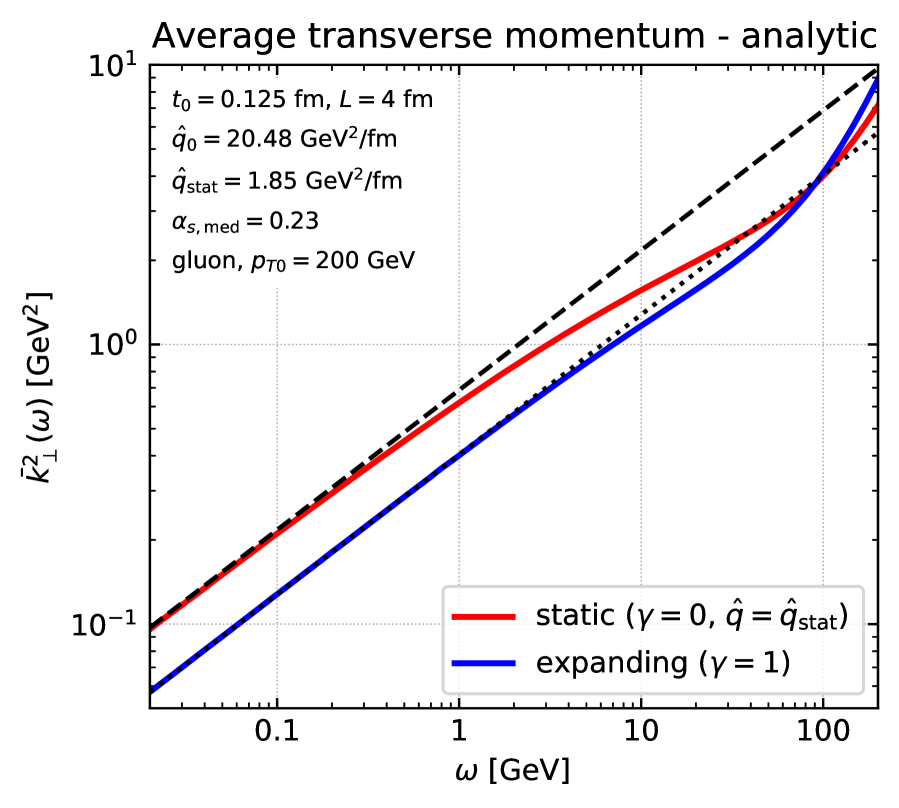
(b) Average transverse momentum squared acquired by a parton in a (purely gluonic) medium induced cascade, in two scenarios: expanding medium (blue) and equivalent static medium (red). The curves are obtained by numerically evaluating Eq. (33).

Figure 2: Scaling violations induced by transverse momentum broadening in medium-induced cascades. For all these results, the jet is triggered by a leading gluon with energy $p_{T0}=200$ GeV.

Fig. 2(a) shows this distribution for the expanding medium with $\gamma=1$ (the blue curve) and for the “equivalent” static medium (the red curve labelled $\gamma=0$), for our default set of parameters (the boldface line in table 1). One sees that for sufficiently high energies $\omega\gtrsim 5$ GeV, the static and expanding results are indistinguishable from each other, indicating perfect scaling. The narrow peak at $\omega\sim p_{T0}$ represents the leading gluon, the minimum at $\omega\sim\tilde{\omega}_{c}$ corresponds to the upper bound on the radiation spectrum, and the increase with decreasing $\omega$ below $\tilde{\omega}_{c}$ is the expected growth $\propto 1/\sqrt{\omega}$, cf. Eq. (12). However, the scaling is broken at lower energies $\omega\lesssim 5$ GeV, where both distributions show a broad peak.

These features are easy to understand. Partons with large $\omega$ remain inside the jet even after transverse momentum broadening, hence their energy spectrum is independent of the jet radius $R$ and scaling is obeyed. On the contrary, momentum broadening can deflect softer gluons to angles $\theta\simeq k_{\perp}/\omega$ larger than $R$. This explains both the decrease of $D(\omega)$ at low energies and the scaling violations, as we now explain.

To that aim, we rely on the analysis of transverse momentum broadening in section 2.6. The broad peak visible in Fig. 2(a) at intermediate energies corresponds to the softest gluons whose propagation angle is still inside the jet: $\theta\simeq k_{\perp}/\omega\lesssim R$, or $\omega\gtrsim k_{\perp}/R$. From Fig. 2(a), one sees that the relevant energies are comparable to the medium scale $\omega_{\textrm{br}}\simeq 3.35$ GeV for multiple branching, cf. table 1. For these gluons, the average transverse momentum $\bar{k}_{\perp}^{\,2}(\omega)$ is controlled by $\hat{q}(L)$ for the expanding medium, and by $\hat{q}_{\rm stat}$ for the “equivalent” static one (see the discussion towards the end of Sect. 2.6 and in Appendix A). Since $\hat{q}(L)<\hat{q}_{\rm stat}$, $\bar{k}_{\perp}^{\,2}(\omega)$ is smaller (for a given energy $\omega\lesssim\omega_{\textrm{br}}$) in an expanding medium than in the equivalent static one. This is illustrated by the plot in Fig. 2(b), which shows numerical results for $\bar{k}_{\perp}^{\,2}(\omega)$ for the two scenarios, as obtained via the method outlined in Appendix A . Because of that, the soft gluons are more likely to remain within the jet cone in an expanding-medium than in the corresponding static one. In particular, the position of the low-energy peak in the spectrum can be roughly estimated as $\bar{\omega}\simeq\bar{k}_{\perp}(\bar{\omega})/R$. This implicit equation gives a result $\bar{\omega}\simeq(\hat{q}/16\bar{\alpha}_{s}^{2}R^{4})^{1/3}$ which is smaller for the expanding medium than for the static one (because $\hat{q}(L)<\hat{q}_{\text{stat}}$), in agreement with Fig. 2(a).

4.3 Energy loss by the leading parton via MIEs

For phenomenological applications, it is interesting to understand the average energy, $\varepsilon(p_{T0},R)$, lost by a jet initiated by a hard parton of momentum $p_{T0}$ outside a cone of opening angle $R$. We cover the case with only MIEs in this section and discuss the case of a full parton shower, including both VLEs and MIEs, in the next section.

Within our effective theory, $\varepsilon(p_{T0},R)$ is the sum of two components Blaizot:2013hx ; Fister:2014zxa : (i) the energy flowing down to arbitrarily soft energies (hence, moving out to arbitrarily large angles), via multiple branchings; this corresponds to the “turbulent flow” in the language of Refs. Blaizot:2013hx ; Fister:2014zxa and gives a contribution proportional to $\omega_{\textrm{br}}$, and (ii) the energy carried by primary emissions which are soft enough to propagate at angles larger than $R$, i.e. gluons with energies $\omega\lesssim\bar{\omega}$, with $\bar{\omega}\simeq\big{(}\hat{q}(L)/16\bar{\alpha}_{s}^{2}R^{4}\big{)}^{1/3}$ the scale introduced at the end of section 4.2. Altogether, we can write

$$\varepsilon(p_{T0},R)\simeq\upsilon\omega_{\textrm{br}}+\int_{0}^{\bar{\omega}}{\rm{d}}\omega\,\omega\frac{{\rm{d}}N}{{\rm{d}}\omega}$$ (19)

with $\upsilon$ a constant. While the first component, inclusive in $k_{\perp}$, satisfies the scaling behaviour w.r.t. the equivalent static medium, the second component breaks the scaling through the upper limit $\bar{\omega}$ which comes from the transverse momentum broadening (see section 4.2). Since $\bar{\omega}_{\rm exp}<\bar{\omega}_{\rm stat}$ (with obvious notations), the partonic energy loss $\varepsilon(p_{T0},R)$ is expected to be smaller in the expanding scenario. This is another consequence of the fact that soft emissions are more likely to remain inside the jet in an expanding medium.

To verify this and to check the functional dependence predicted by Eq. (19), we compute the average energy loss $\varepsilon(p_{T0},R)$ for a gluon initiated jet and for various values of the initial energy $p_{T0}$ and the jet radius $R$, using again our default set of medium parameters. The results are shown as dotted lines in Fig. 3, for both the expanding medium (blue curves) and the equivalent static one (blue curves). While they confirm that the energy loss is slightly smaller for an expanding medium, the differences are barely visible, corresponding to an almost perfect scaling.

To better understand this, we consider the scaling violations induced by the upper limit $\bar{\omega}$ in the second term in Eq. (19). Using $\omega({\rm{d}}N/{\rm{d}}\omega)\propto 1/\sqrt{\omega}$, cf. Eq. (12), one sees that this term scales like $\bar{\omega}^{1/2}\propto\hat{q}^{1/6}$. The contribution from this second term will therefore be larger for the static medium only by a moderate factor of $(\hat{q}_{\rm stat}/\hat{q}(L))^{1/6}\simeq 4^{1/6}\simeq 1.26$.

The dotted lines in Fig. 3(b) show the dependence of $\varepsilon(p_{T0},R)$ on $R$ (for fixed $p_{T0}=200$ GeV), for the two scenarios for the medium. This dependence comes from the upper limit $\bar{\omega}$ in the integral term of Eq. (19), with $\bar{\omega}^{1/2}\propto R^{-2/3}$. (As expected on physical grounds, $\varepsilon(p_{T0},R)$ saturates at large $R$.) We have checked that this particular law is in good numerical agreement with the numerical results in Fig. 3(b). Once again the scaling is almost perfect.

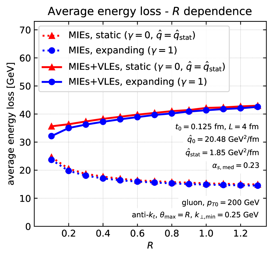
(a)

(b)

Figure 3: Our MC results for the average energy loss by a gluon-initiated jet are displayed as a function of the initial energy $p_{T0}$ of the leading parton (left) and the jet radius $R$ (right), for two scenarios for the jet evolution: jets with MIEs only (dotted lines) and full showers with both MIEs and VLEs (plain lines). For each scenario, we compare the case of an expanding medium (blue) with the equivalent static one (red).

4.4 Scaling violations and energy loss for full in-medium parton shower

As explained at length in section 2.1 (see Caucal:2019uvr for additional details), the VLEs radiated inside the medium act as new partonic sources for MIEs. Each of these new sources will therefore contribute to the overall energy lost by the jet (via radiation of MIEs at angles $\theta>R$). This results in a significant increase of the total jet energy loss, compared to that of a single parton evolving via MIEs only. In this case, it is important to consider the energy lost by the jet as a whole instead of the energy lost by just the leading parton. In this section, we study how our results from Ref. Caucal:2019uvr are modified by the expansion of the medium, notably in the context of the scaling relation derived in section 4.1.

As discussed in Sect. 2 (see Fig. 1), in the presence of the longitudinal expansion, the energies and the emissions angles of the VLEs occurring inside the medium are constrained by Eq. (4) and $\theta\geq\theta_{c}=2/\sqrt{\hat{q}(L)L^{3}}$. Together with the medium-size boundary, $\omega=\omega_{L}(\theta)\equiv 2/(L\theta^{2})$, this defines the intersection point at $\omega=\omega_{c}$ and $\theta=\theta_{c}$, cf. (5). The corresponding boundaries and intersection point for the “equivalent” static medium are obtained by replacing $\gamma$ by $0$ and $\hat{q}(L)$ by $\hat{q}_{\rm stat}$, with $\hat{q}_{\rm stat}$ given by Eq. (17).

In practice, we define the total jet energy loss as difference between the energy of the initial hard parton, $p_{T0}$, and the the energy of the final reconstructed jet after evolving the hard parton including both VLEs and MIEs. To make sure this includes only the medium-induced energy loss, and not also vacuum-like emissions outside the jet, we subtract the equivalent average energy loss computed on vacuum jets. Our results for the full-jet energy loss are shown by the solid lines in Fig. 3. The main trend, for both static and expanding media, is a steady growth of the jet energy loss with the initial energy $p_{T0}$ and with the radius $R$, due to the increase of the phase-space for in-medium VLEs with both $p_{T0}$ and $R$.

Fig. 3 also shows a slight decrease of the energy loss for an expanding medium ($\gamma=1$) compared to the equivalent static one ($\gamma=0$). This reduction becomes sizeable only for large initial energy $p_{T0}\gtrsim 200$ GeV and/or very small values for the jet radius $R\lesssim 0.2$. A priori, these scaling violations may have two sources: the $k_{\perp}$-broadening discussed in section 4.2 and the different phase-space available to VLEs inside the medium. The smaller difference between the dotted lines than between the solid lines in Fig. 3 already suggests that the second effect — the difference in the phase-space for VLEs — dominates over the former. We study this effect in more details below.

Strictly speaking, both the slope of the boundary in (4) and the coordinates of the intersection point, differ between the two scenarios. However, within our leading logarithmic approximation for the VLEs, only the ($\gamma$-dependent) change in the slope is under control: multiplying $\omega_{0}(\theta)$ and $\omega_{L}(\theta)$ by an arbitrary numerical prefactor of order one does not affect the overall leading-logarithmic accuracy (recall the discussion in the paragraph after Eq. (3)). In particular, at double-logarithmic accuracy, we could have chosen the prefactor in Eq. (4) such that the intersection point be given by (5) with $\hat{q}(L)\to\hat{q}_{\rm stat}$ for both the expanding and the static media, or, conversely, constructed the static medium with $\hat{q}=\hat{q}(L)$.

That said, the difference in slopes between the two scenarios does matter at double-logarithmic accuracy. Using Eq. (4), one can easily check that this difference is such that the phase-space available for in-medium VLEs is smaller for an expanding medium than for the “equivalent” static one (see Fig. 1). Therefore, the number of VLEs inside the medium, and hence of sources for MIEs, is smaller for an expanding medium, resulting in a smaller jet energy loss.

(a) Monte-Carlo simulations

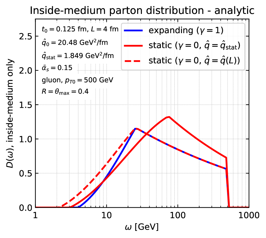
(b) Analytic (DLA) results

Figure 4: Parton energy distribution $D(\omega)\equiv{\omega(\rm d}N/{\rm d}\omega)$ in a parton shower exclusively generated via VLEs inside the medium: (a) Monte Carlo simulations; (b) analytic results within the double-logarithmic approximation with fixed coupling. The leading parton is a gluon with $p_{T0}=500$ GeV and the jet radius is $R=0.4$. The solid blue lines correspond to the an expanding medium with $\gamma=1$; the red lines correspond to a static ($\gamma=0)$ medium, with either $\hat{q}=\hat{q}_{\text{stat}}$ (solid lines), or $\hat{q}=\hat{q}(L)$ (dashed lines). The contribution from the leading parton (a peak at $\omega\simeq p_{T0}=500$ GeV) is not included in the analytic plot.

To make this argument more concrete, we can directly look at the energy ($\omega$) distribution of the partons produced only via VLEs inside the medium (i.e. without MIEs and without the VLEs outside the medium). Fig. 4 shows our results, for an initial parton of 500 GeV. Fig. 4(a) is the result of our Monte Carlo simulations and Fig. 4(b) is the result of the analytic calculation in the double-logarithmic approximation (more details below). Each plot includes three curves: the solid blue line corresponds to an expanding medium, with $\gamma=1$ and our default medium parameters; the two red curves correspond to two different choices for a static medium, with different transport coefficients: $\hat{q}=\hat{q}_{\text{stat}}$, cf. Eq. (17) (solid red line), and $\hat{q}=\hat{q}(L)$ (dashed red line). This last choice gives the same values of $\omega_{c}$ and $\theta_{c}$ as in the expanding medium.

In all cases, one sees a peak at large $\omega$ corresponding to the leading parton, together with a continuous distribution extending towards smaller $\omega$. More importantly, we see a global increase in the number of sources in both static media compared to the expanding one. This ultimately yields the larger energy loss observed in the full MC simulations, as shown by the solid lines in Fig. 3. This is more striking for the static medium where the values of $\omega_{c}$ and $\theta_{c}$ have been chosen to agree with the expanding medium, the red dashed line inf Fig. 4. In this case, the static and expanding cases agree almost perfectly at high $\omega$ ($\omega\gtrsim\omega_{c}=25.6$ GeV). For $\omega\lesssim\omega_{c}=25.6$ GeV, the expanding medium yields a distribution which is more suppressed than for the static one with $\hat{q}=\hat{q}(L)$, due to the different slope of the phase-space boundary.

We finally explain our analytic results in Fig. 4(b). We start from the double-differential distribution in $\omega$ and $\theta$ computed in our first paper Caucal:2018dla ,

$$T(\omega,\theta)=\omega\theta^{2}\,\frac{{\rm d}^{2}N}{{\rm d}\omega\,{\rm d}\theta^{2}}=\bar{\alpha}_{s}\textrm{I}_{0}\left(2\sqrt{\bar{\alpha}_{s}\ln\frac{p_{T0}}{\omega}\ln\frac{R^{2}}{\theta^{2}}}\right),$$ (20)

with $\textrm{I}_{0}$ the modified Bessel function of rank 0. This result is valid in the vacuum and in the fixed-coupling limit. The inside-medium $\omega$ spectrum is obtained by integrating (20) over $\theta$ with the constraint that the emission occurs inside the medium, i.e. satisfies both Eq. (4) and $\theta>\theta_{c}$. The former constraint dominates for $\omega<\omega_{c}$, while the latter dominates above $\omega_{c}$. One finds

$$D(\omega)\equiv\omega\,\frac{{\rm d}N}{{\rm d}\omega}\simeq\sqrt{\bar{\alpha}_{s}\frac{L_{\text{min}}}{\ln\frac{p_{T0}}{\omega}}}\,\textrm{I}_{1}\left(2\sqrt{\bar{\alpha}_{s}\ln\frac{p_{T0}}{\omega}L_{\text{min}}}\right),$$ (21)

with $\textrm{I}_{1}$ the modified Bessel function of rank 1 and

$$L_{\text{min}}\equiv\begin{cases}\ln\frac{R^{2}}{\theta_{c}^{2}}&\text{ if }\omega>\omega_{c},\\[5.69046pt] \frac{1}{2-\gamma}\ln\frac{\omega^{3-\gamma}R^{4-2\gamma}}{2^{1-\gamma}\hat{q}_{0}t_{0}^{\gamma}}&\text{ if }\omega<\omega_{c}.\end{cases}$$ (22)

This is the result plotted in Fig. 4(b), with an additional contribution $\delta(\omega-p_{T0})$ from the leading parton omitted. The analytic calculation captures, at least qualitatively, the features seen in the Monte Carlo simulation, cf. Fig. 4(a).

5 Jet quenching phenomenology in a longitudinally-expanding medium

In this last section, we present MC simulations for three standard jet observables in ultra-relativistic heavy ion collisions: the nuclear modification factors for inclusive jet production, the jet fragmentation function, and the $z_{g}$ and $\theta_{g}$ distribution obtained with the Soft Drop substructure tool. Our aim is twofold. On one hand, we would like to gauge the impact of the medium expansion on the selected observables, by comparing it with the corresponding predictions of the “equivalent” static-medium scenario. On the other hand, we would like to demonstrate that adding the longitudinal expansion to the general picture presented in Caucal:2018dla still provides as good a phenomenological description of these observables as that obtained for a static medium in Caucal:2019uvr ; Caucal:2020xad . As in these latter studies, it is not our intention here to provide realistic fits of the experimental data, but merely to show that overall physical picture explains the salient features visible in these data.

5.1 The nuclear modification factor for jets $R_{AA}$

We start by computing the nuclear modification factor for the inclusive jet cross-section, $R_{AA}$, as a function of the jet transverse momentum $p_{T}$, following the ATLAS set-up Aaboud:2018twu .

Compared to our earlier work in Caucal:2019uvr , we have included in our simulation the effect of the nuclear PDF effects, which have been argued in Pablos:2019ngg ; Huss:2020dwe to have a sizeable impact on $R_{AA}$ especially at large $p_{T}$. In practice, this is done by adding the EPPS (NLO) nuclear PDFs corrections Eskola:2016oht to the Born-level matrix elements used in our medium Monte Carlo medium simulations. Currently, these corrections are afflicted by large uncertainties, but in our MC calculations we have solely included their central values. Indeed, we have checked that the associated uncertainties could be absorbed into (slight) modifications of our free parameters, while still keeping them within physically reasonable ranges.

The red dotted curve in Fig. 5(a) shows the effect on $R_{AA}$ of the nuclear PDFs alone, i.e. without any final-state quenching: the hard process is weighted by the nuclear PDFs, but the subsequent jet evolution occurs as in the vacuum. At large $p_{T}\gtrsim 500$ GeV, the nuclear PDFs tend to reduce the jet cross-section by $\sim 20\%$. This is likely a consequence of the EMC effect Malace:2014uea i.e. of the suppression of the quark PDF at large $x$ in nuclei compared to nucleons. Even if this initial-state effect is sizeable, we remind the reader that, in our picture, the crucial ingredient explaining the flatness of $R_{AA}$ at high $p_{T}$ is the increase of the average energy loss by the jets, due to the increase in the number of partonic sources produced via VLEs inside the medium Caucal:2019uvr . This effect per se (without nuclear PDFs effects) was sufficient to provide a good description of the ATLAS data Aaboud:2018twu (within their uncertainty), as shown in Caucal:2019uvr . The inclusion of the nuclear PDF effects provides a further reduction at large $p_{T}$, significantly improving the agreement with the ATLAS data.

(a) Effects of the nuclear PDFs alone (red dotted curve) and comparison between expanding and equivalent static medium (solid and dotted blue lines, respectively).

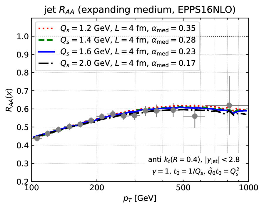
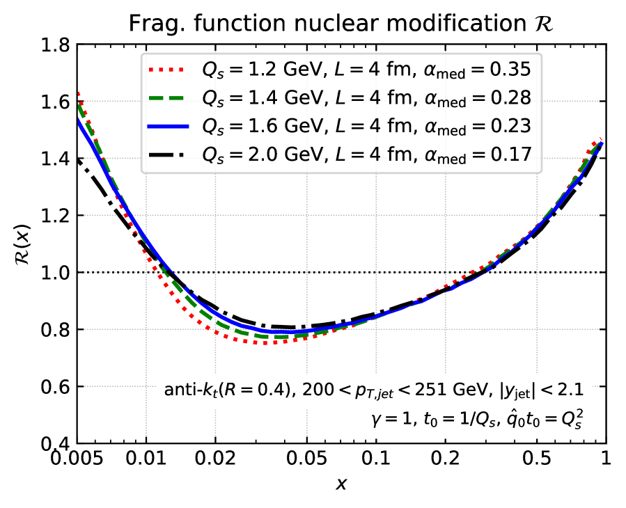
(b) MC results for an expanding medium ($\gamma=1$) and nuclear PDFs vs. the ATLAS data Aaboud:2018twu . The 4 sets of medium parameters displayed in this plot (cf. table 1) provide almost identical predictions.

Figure 5: Monte-Carlo simulations for the nuclear modification factor $R_{AA}$ for inclusive jet production.

To isolate the effect of the medium expansion on $R_{AA}$, we show in Fig. 5(a) the results of two MC simulations (both including the nuclear PDFs): one for a longitudinally-expanding medium with $\gamma=1$, $Q_{s}=1.6$ GeV, $L=4$ fm and $\alpha_{s,\rm med}=0.23$ (our default set of medium parameters, see the third line in table 1) and the other one for the “equivalent” static medium, with $\hat{q}_{\rm stat}$ given by Eq. (17) and $L_{\rm stat}=L-t_{0}$.

The numerical results in Fig. 5(a) show only a mild difference between the two scenarios, with $R_{AA}$ being slightly larger for the expanding medium than for the static one and the difference increasing slowly with the jet $p_{T}$. Since the jet $R_{AA}$ is mainly controlled by the jet energy loss, this is in agreement with our previous discussion of the scaling violations in Sect. 4 (see Fig. 3(a)) where we observed a smaller average jet energy loss for the full in-medium parton shower for an expanding medium compared to the equivalent static one, with a stronger effect at large $p_{T}$. The fact that the net effect of the longitudinal expansion can be so well reproduced by an effective static-medium scenario a posteriori explains why it has been possible in Caucal:2019uvr to provide a rather good description of the ATLAS data for $R_{AA}$ within an oversimplified model assuming a static medium.

Let us now focus on more phenomenological studies of the $R_{AA}$ factor for a longitudinally-expanding medium. Fig. 5(b) compares our Monte-Carlo predictions for each of the four sets of medium parameters introduced in table 1 to the ATLAS measurement, showing an excellent agreement. For each set of parameter, the value of ${\alpha}_{s,\text{med}}$ has been (manually) adjusted to give a good description of the data. For simplicity, we have only varied $Q_{s}$, setting $t_{0}=1/Q_{s}$ and $\hat{q}_{0}t_{0}=Q_{s}^{2}$, keeping $\gamma=1$ and $L=4$ fm. These last two parameters could have been varied as well.

The physical reason behind this degeneracy in our theoretical description of $R_{AA}$ has been explained in detail in Caucal:2019uvr . In a nutshell, $R_{AA}$ is mainly sensitive to the energy loss via soft MIEs at large angles, i.e. to the branching scale $\omega_{\textrm{br}}=\bar{\alpha}_{s,\rm med}^{2}\hat{q}_{\rm stat}L^{2}$. However, variations of the in-medium phase space for vacuum-like sources associated with variations of $\hat{q}_{0}$ and $t_{0}$ (through $Q_{s}$) can compensate the variations of $\omega_{\textrm{br}}$ through $\alpha_{s,\rm med}$. At this point, it is interesting to observe that the value of $\alpha_{s,\rm med}$ which is preferred by our phenomenological description of the $R_{AA}$ data is monotonously decreasing with increasing $Q_{s}$, in qualitative agreement with the property of asymptotic freedom. (Indeed, increasing $Q_{s}$ is tantamount to increasing the density of the medium, as obvious from the fact that $\hat{q}_{0}=Q_{s}^{3}$.)

5.2 Jet fragmentation function

We turn now to the discussion of the jet fragmentation function $\mathcal{D}(x)=\frac{1}{N_{\textrm{jets}}}\frac{{\rm{d}}N}{{\rm{d}}x}$, defined as the multiplicity of hadrons inside the jets per unit of longitudinal momentum fraction $x\equiv p_{T}\cos(\Delta R)/p_{T,\rm jet}$. Here, $p_{T}$ and $\Delta R$ are respectively the transverse momentum and the angle with respect to the jet axis of the measured hadron, while $p_{T,\rm jet}$ is the jet total transverse momentum. We denote by $\mathcal{R}(x)\equiv\mathcal{D}^{\rm med}(x)/\mathcal{D}^{\rm vac}(x)$ the associated nuclear modification factor. The jet selection used in our MC analysis closely follows the experimental analysis by the ATLAS collaboration in Aaboud:2018hpb .

In a previous paper Caucal:2020xad , we have studied the nuclear modification of the fragmentation function within our pQCD picture for the case of a static medium. To understand the effect of the longitudinal expansion on this observable, it is again enlightening to compare our MC results for $\mathcal{R}(x)$ for the case of an expanding medium and for the “equivalent” static medium. This comparison is shown in Fig. 6(a), for our default set of values for the free parameters (cf. the bold line in Table 1).

The dotted red curve in this figure corresponds to a calculation which includes the nuclear PDFs in the initial state, but no medium effects in the final state, in analogy with the dotted red curve in Fig. 5(a). Unlike in the case of $R_{AA}$, it appears that the nuclear PDFs have no effect on the jet fragmentation function. This is likely related to the fact that the jet transverse momenta involved in the present calculation of $\mathcal{R}(x)$ are relatively low, $200\leq p_{T,\rm jet}\leq 251$ GeV.

Our MC results for $\mathcal{R}(x)$, including both nuclear PDFs and the in-medium effects, are represented by the plain blue curve for the Bjorken-expanding medium and by the dotted blue curve for the equivalent static medium. As for $R_{AA}$, the scaling looks nearly exact. At large $x\gtrsim 0.2$, the fragmentation function enhancement ($\mathcal{R}(x)>1$) has been shown in Ref. Caucal:2020xad to be controlled by the energy loss by the jet together with the bias introduced by the steeply falling initial spectrum which favours jets losing less energy than average. The almost-perfect scaling for the fragmentation at large $x$ therefore stems from the equivalent almost-perfect scaling seen for $R_{AA}$ in Fig. 5(a). This is a rather universal feature, that has been argued in model-independent phenomenological studies Spousta:2015fca and is indeed verified in a variety of theoretical descriptions, from weak to strong coupling Milhano:2015mng ; KunnawalkamElayavalli:2017hxo ; Chesler:2015nqz ; Rajagopal:2016uip ; Casalderrey-Solana:2016jvj ; Casalderrey-Solana:2018wrw ; Casalderrey-Solana:2019ubu .

The rather good scaling visible in Fig. 6(a) at small $x\lesssim 0.02$ is likely to be fortuitous: within our effective theory at least, it is the result of the compensation between two scaling-violating effects, which act in opposite directions. As argued in Caucal:2020xad , the small-$x$ part of the medium-modified fragmentation function is controlled by the multiplicity of in-medium VLEs and by the number of MIEs that remain inside the jet cone after crossing the medium. The latter effect tends to increase in an expanding medium compared to the equivalent static one since the transverse momentum broadening decreases (cf. Fig. 2(b) and the discussion in Sect. 4.2). The former effect decreases in the expanding medium since the associated phase-space is smaller than for the equivalent static medium (cf. Sect. 4.4). The net effect visible in Fig. 6(a) turns out to be a mild increase.

(a) Effects of the nuclear PDFs alone (nearly-horizontal, red, dotted curve) and comparison between expanding and equivalent static medium (solid and dotted blue lines, respectively).

(b) MC results for a Bjorken-expanding medium with $\gamma=1$ and for the 4 sets of medium parameters summarised in table 1.

Figure 6: Monte-Carlo calculation of the nuclear modification factor for the jet fragmentation function.

Turning to a more phenomenological analysis, we exhibit in Fig. 6(b) our MC results for the nuclear modification factor $\mathcal{R}(x)$ for jet fragmentation, for the same four sets of medium parameters in table 1 that were already shown in Fig. 5(b) to offer a good description for the ATLAS data for $R_{AA}$. At large $x\gtrsim 0.2$, the four curves are nearly overlapping with each other, a property associated in Caucal:2020xad with the strong correlation between hard-fragmenting jets and $R_{AA}$. At the small-$x$ end of the spectrum, the dispersion between the different curves is more pronounced albeit still small. This reflects the complexity of the physical mechanisms at work in that regime.

In view of the theoretical uncertainties inherent to our current framework, which are especially important for the fragmentation function at small $x$ (see again Caucal:2020xad ), we do not show an explicit comparison between our results and the LHC data for nuclear effects on jet fragmentation. That said, it is reassuring to observe that all our curves in Fig. 5(b) show the same qualitative features as the respective data (see e.g. Aaboud:2018hpb ), that is, a pronounced nuclear enhancement at both small $x$ and large $x$, together with a nuclear suppression at intermediate values of $x$.

5.3 Jet substructure observables

To conclude this survey of jet quenching observables in a longitudinally expanding medium, we study the Soft Drop $z_{g}$ and $\theta_{g}$ distributions Larkoski:2014wba ; Larkoski:2015lea for $\beta=0$, and their respective nuclear modification factor $\mathcal{R}(z_{g})$, $\mathcal{R}(\theta_{g})$. Being infrared and collinear safe ($\theta_{g}$) or at least Sudakov-safe ($z_{g}$, see Ref. Larkoski:2015lea ), these observables are expected to be better-controlled in perturbation theory than the fragmentation function. In particular, they are less sensitive to non-perturbative hadronisation corrections which are not included in our Monte Carlo. For brevity, we only show results for the longitudinally-expanding medium with $\gamma=1$. We have however checked that the scaling between an expanding medium and the equivalent static one works well for these substructure observables,

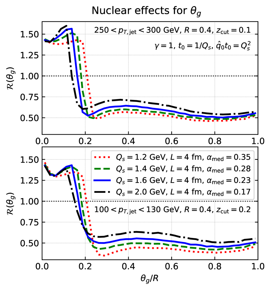
(a) $\theta_{g}$ distributions.

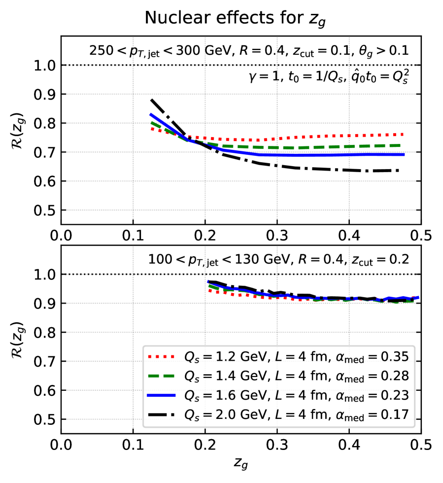
(b) $z_{g}$ distributions.

Figure 7: Monte-Carlo simulations of the nuclear modification factor for distributions after Soft Drop: (a) the groomed jet radius $\theta_{g}$ and (b) the momentum fraction $z_{g}$. The Soft Drop parameter $\beta$ is set to $\beta=0$. For both distributions, the upper panel corresponds to $z_{\rm cut}=0.1$ and $250<p_{T,\rm jet}<300$ GeV, whereas the lower panel has $z_{\rm cut}=0.2$ and $100<p_{T,\rm jet}<130$ GeV. As in the ALICE Acharya:2019djg and CMS measurements Sirunyan:2017bsd , an additional angular cut-off $\theta_{g}>0.1$ is imposed for the $z_{g}$ distribution calculated with $z_{\rm cut}=0.1$. We use the same sets of values for the medium parameters as in Figs. 5(b)–6(b) (cf. table 1).

Let us first consider the groomed $\theta_{g}$ distribution shown in Fig. 7(a) for two choices for the jet selection in $p_{T,\rm jet}$ and for the Soft Drop parameter $z_{\textrm{cut}}$: $250<p_{T,\rm jet}<300$ GeV and $z_{\textrm{cut}}=0.1$ (upper panel), and, respectively, $100<p_{T,\rm jet}<130$ GeV and $z_{\textrm{cut}}=0.2$ (lower panel). In both cases, one observes a suppression of large–$\theta_{g}$ jets and an enhancement of small–$\theta_{g}$ jets, with the transition between the two types of behaviour occurring slightly below $\theta_{g}=0.1$ (i.e. for $\theta_{g}/R\sim 0.2$).

This behaviour indicates that the opening angle distribution for jets emerging from the plasma within any specified range of energies has been pushed toward smaller angles, comparing to $pp$ jets with the same energies. This trend is a rather generic feature, which has been observed in a variety of theoretical descriptions, at both weak Ringer:2019rfk and strong coupling Chesler:2015nqz ; Rajagopal:2016uip , and also in hybrid models Casalderrey-Solana:2014bpa ; Hulcher:2017cpt ; Casalderrey-Solana:2019ubu . The ultimate reason for this narrowing of jets in the medium is that small-angle jets suffer less energy loss and jets with a higher initial energy are less frequent (due to the steeply falling initial spectrum).

To understand our results in Fig. 7(a) in more detail and, in particular, the peculiar transition occurring around $\theta_{g}=0.1$, it is important to elucidate the precise mechanisms relating the (sub)jet angular opening to energy loss in our picture. There is first a rather generic mechanism, present in all pQCD-based approaches: the medium introduces a bias towards quark-initiated jets, which lose less energy than the gluon jets, thus leading to a narrowing of the angular distribution Ringer:2019rfk , since quark jets are “narrower” than gluon jets. Conversely, the transverse broadening of the two subjets selected by Soft Drop leads to a widening of the $\theta_{g}$ distribution Ringer:2019rfk . This effect too is present in our MC calculations but turns out to be numerically small.

The dominant mechanism behind the sharp transition observed in the $\theta_{g}$–distribution in Fig. 7(a) is colour decoherence and the associated angle $\theta_{c}$, cf. Eq. (5). The physical picture is as follows: when the two subjets selected by Soft Drop have an angular separation $\theta_{g}>\theta_{c}$, each subjet loses energy independently, whereas when $\theta_{g}<\theta_{c}$ the energy is lost by the parent subjet. Since the jet energy loss increases with the number of partonic sources for MIEs, jets with $\theta_{g}>\theta_{c}$ lose more energy than jets with $\theta_{g}<\theta_{c}$. This explains the suppression of the $\theta_{g}$ distribution for $\theta_{g}>\theta_{c}$ and the enhancement for $\theta_{g}<\theta_{c}$. This shows that the medium acting as a filter towards coherent jets, by reducing the number of two-prongs jets with $\theta_{g}\gg\theta_{c}$. A similar mechanism is also present in strong coupling models, where the role of the coherence angle is played by the plasma resolution length Casalderrey-Solana:2014bpa ; Hulcher:2017cpt ; Casalderrey-Solana:2019ubu . Numerically, the transition in Fig. 7(a) is indeed seen at $\theta_{g}\simeq\theta_{c}$, with $\theta_{c}$ varying between $0.08$ and $0.05$ when $Q_{s}$ varies between $1.2$ GeV and $2$ GeV, cf. table 1, including the expected shift of the transition point towards smaller $\theta_{g}$ when $\theta_{c}$ decreases ($Q_{s}$ increases).

On the experimental side, the narrowing of jets in the medium has been measured by the ALICE collaboration Mulligan:2020cnp . The results are in qualitative agreement with our theoretical predictions shown Fig. 7, as a suppression of large–$\theta_{g}$ jets and an enhancement of small–$\theta_{g}$ jets are clearly visible in spite of the large statistical uncertainties. The transition in the data occurs around $\theta_{g}/R\approx 0.2\div 0.3$ and it does not look as sharp as in our MC results in Fig. 7(a). This should be expected, given that the experimental results represent an average over various medium geometries (hence, over various values for $\theta_{c}$). Besides, also on the theory side, we expect that the sharpness of the transition will be smoothed out by subleading perturbative contributions and additional effects like hadronisation, not yet included in our simulations. The above discussion however suggests that a more precise measurement of the $\theta_{g}$ distribution at small $\theta_{g}\ll R$ could give us a direct experimental access to the plasma coherence angle $\theta_{c}$, at least in an average sense.

Finally, the groomed $z_{g}$–distribution in a Bjorken-expanding medium is presented Fig. 7(b) for the same two choices of jet selection and Soft Drop parameters as for the $\theta_{g}$–distributions in Fig. 7(a). For the upper panel we have imposed the additional restriction that the groomed angle should satisfy $\theta_{g}>\theta_{\rm cut}=0.1$, as is common in several experimental analyses. Within our pQCD picture, the physical content of the $z_{g}$ distribution has been explored in Caucal:2019uvr for the case of a static medium. The medium expansion does not change the physical mechanisms at the origin of the nuclear modifications. The overall suppression of the distribution, i.e. the fact that $\mathcal{R}(z_{g})<1$ for all values of $z_{g}$, is again a consequence of the in-medium suppression of jets having a large-angle hard substructure. This suppression is therefore less pronounced for inclusive $\theta_{g}$ jets (lower panel) than for jets with $\theta_{g}>0.1$ (upper panel). On the other hand, the increase of $\mathcal{R}(z_{g})$ when decreasing $z_{g}$, especially below $z_{g}\sim 0.2$, is due to relatively hard MIEs triggering the Soft Drop condition. As visible in the upper panel, this increase becomes more pronounced as $Q_{s}$ increases (for $L$ fixed). This is so since $\theta_{c}=2/(Q_{s}L)$ decreases with increasing $Q_{s}$ (see also table 1), meaning that the relatively hard emissions with $\theta\sim\theta_{c}$ are more likely to remain inside the jet cone. Additionally, $\omega_{c}=\frac{1}{2}Q_{s}^{2}L$ increases with increasing $Q_{s}$, making MIEs more likely to pass the Soft Drop $z_{\text{cut}}$ condition.

6 Conclusion

In this paper, we have extended our pQCD approach to the evolution of a jet in a dense quark-gluon plasma, as developed in Refs. Caucal:2018dla ; Caucal:2019uvr ; Caucal:2020xad , to the case of a medium which undergoes longitudinal expansion. We have demonstrated that the factorisation in time between vacuum-like emissions and medium-induced emissions remains valid in the expanding plasma and established the new phase space for in-medium VLEs to leading logarithmic accuracy. Regarding the medium-induced radiation, we have focused on the relatively soft emissions with energies $\omega\ll\omega_{c}$, for which the emission process can be approximately treated as local in time. This locality allowed us to absorb the medium expansion into an effective emission rate which involves the value of the jet quenching parameter at the time of the emission. Our Monte Carlo parton shower, initially designed for a static plasma Caucal:2019uvr , has been extended to take into account the three main modifications introduced by the longitudinal expansion, namely, the modified phase space for VLEs, the change in the rate for transverse momentum broadening, and that in the emission rate for MIEs.

From a conceptual point of view, we have made the elementary, yet important, observation, that the locality of soft MIEs leads to exact scaling properties between expanding and static media for the parton energy distributions (integrated over the emission angles) in medium-induced cascades. This has allowed us to define an “equivalent static medium” for a given expanding scenario, with the equivalence being strictly true for MIEs only. We have used this “equivalent” static medium as a benchmark for “apple-to-apple” comparisons between the jet properties (energy loss, intra-jet multiplicities, jet substructure) for an expanding and a static medium, respectively. Our key result is that the scaling property is only mildly violated by processes which have a different scaling with $\hat{q}(t)$, such as the transverse momentum broadening via multiple soft scattering, or the phase-space for VLEs occurring inside the medium (which act as sources for medium-induced radiation).

On the phenomenological side, we have presented new Monte Carlo simulations for the case of an expanding plasma, which cover the nuclear modification factors for inclusive jet production (the jet $R_{AA}$), the jet fragmentation function, and the Soft Drop distributions in the groomed radius $\theta_{g}$ and the momentum sharing fraction $z_{g}$. The good qualitative agreement that we previously found between these jet observables computed in a static medium and the LHC data turns out to remain in place after including the medium expansion. This is so because of the mildness of the scaling violations w.r.t. the “equivalent” static medium. This consolidates the pQCD foundations of our picture for jet evolution, since it confirms that the salient features of the nuclear effects on all the observables that we have investigated are driven by perturbative effects and are only slightly sensitive to the details of the bulk evolution. Our studies of the jet $R_{AA}$ modification factor also confirm that the inclusion of nuclear PDF effects improve the agreement with the ATLAS data at large $p_{T,\text{jet}}$.

That said, there is still a large room for improvement in our current implementation of an in-medium parton shower. As emphasised in several places, both the collisions inside the medium and the medium-induced radiations are considered as relatively soft. Even though preliminary studies seem to indicate a minor effect on the jet $R_{AA}$, a proper treatment of the single hard scattering regime Gyulassy:2000er and of the medium-induced spectrum at larger energies $\omega\gtrsim\omega_{c}$ (perhaps along the lines of the recent studies in Mehtar-Tani:2019tvy ; Mehtar-Tani:2019ygg ; Barata:2020rdn ) is clearly needed and is a part of our plans for the future. At this point, it is interesting to notice that the scaling relation put forward in Baier:1998yf ; Salgado:2002cd ; Salgado:2003gb ; Adhya:2019qse for the relatively hard ($\omega\gtrsim\omega_{c}$) medium-induced emissions differs from “our” scaling by merely a factor of $2$ (in the value of the transport coefficient for the “equivalent” medium), thus suggesting that the scaling violations may remain small even after including this contribution.

We have intentionally focused on jet observables for which the medium geometry can, to a large extent, be absorbed into an effective jet path length $L$. Incorporating a realistic collision geometry is left for future work, as well as a systematic study of jet observables sensitive to it, such as the centrality dependence of $R_{AA}$, or the dijet asymmetry. Finally, even if perturbative mechanisms seem to drive the medium modifications of jet properties, it is known that bulk-related observables such as the medium response to the jet propagation, or the transverse expansion of the quark-gluon plasma, have a sizeable impact in the soft sector of some observables, notably on the fragmentation function and on the jet shapes Casalderrey-Solana:2016jvj ; Tachibana:2017syd ; KunnawalkamElayavalli:2017hxo ; Chen:2017zte ; Tachibana:2020mtb . Adding all such effects goes far beyond the current implementation of our Monte-Carlo, yet this is clearly needed in order to develop a realistic event generator for the study of jets in heavy-ion collisions. This discussion can be viewed as our road map for the next years.

Appendix A Angular structure of medium-induced cascades in expanding media

In this Appendix, we shall demonstrate the results asserted in Sect. 4 regarding the violation of exact scaling between the expanding scenario and the equivalent static medium, due to transverse momentum broadening in medium-induced cascades. Our subsequent treatment of multiple medium-induced branchings largely follows the corresponding discussion in Refs. Blaizot:2013hx ; Blaizot:2013vha ; Blaizot:2014ula ; Blaizot:2014rla , that we shall extend to the case of an expanding medium by simply replacing $\hat{q}\to\hat{q}(t)$, both in the emission rate and in the rate for diffusion in transverse momentum.

A.1 Exact scaling for $k_{\perp}$-inclusive parton distributions

Let us first explain in more mathematical terms what we mean by this exact scaling. As emphasised in Sect. 4, this scaling property only refers to the parton distribution produced by medium-induced cascades which are inclusive w.r.t. the transverse momentum of emission. The evolution equation for the $k_{\perp}$-inclusive parton distribution at time $t$, $D(x,t)\equiv x{\rm{d}}N/{\rm{d}}x$ is Blaizot:2013hx

$$\frac{\partial D(x,t)}{\partial t}=\bar{\alpha}_{s}\sqrt{\frac{\hat{q}(t)}{E}}\int{\rm{d}}z\,\mathcal{K}(z)\left[\sqrt{\frac{z}{x}}D\left(\frac{x}{z},t\right)-\frac{z}{\sqrt{x}}D(x,t)\right],\qquad\mathcal{K}(z)=\frac{(1-z+z^{2})^{5/2}}{(z(1-z))^{3/2}}.$$ (23)

Without loss of generalities, this equation is written for purely gluonic cascades. The change of variable

$$\tau=\bar{\alpha}_{s}\int_{t_{0}}^{t}{\rm{d}}t^{\prime}\,\sqrt{\frac{\hat{q}(t^{\prime})}{E}}$$ (24)

enables one to rewrite (23) in terms of the dimensionless quantities $\tau$ and $x$:

$$\frac{\partial\widetilde{D}(x,\tau)}{\partial\tau}=\int{\rm{d}}z\,\mathcal{K}(z)\left[\sqrt{\frac{z}{x}}\widetilde{D}\left(\frac{x}{z},\tau\right)-\frac{z}{\sqrt{x}}\widetilde{D}(x,\tau)\right].$$ (25)

Consequently, the solutions of (23) are of the form $D(x,t)=\widetilde{D}(x,\tau(t))$, with $\widetilde{D}(x,\tau)$ a solution of (25). If one fixes the initial time $t_{0}$ and final time $L$ of the evolution, the $k_{\perp}$-inclusive parton distribution in an expanding medium is the same as in a static one provided one has

$$\tau_{\rm exp}(L)=\tau_{\rm stat}(L)\qquad\Longleftrightarrow\qquad\int_{t_{0}}^{L}{\rm{d}}t\,\sqrt{\hat{q}(t)}=\sqrt{\hat{q}_{\rm stat}}(L-t_{0})$$ (26)

giving the condition (17). We refer to Eq. (26) as the scaling relation between expanding and static media with $\hat{q}_{\rm stat}$ the quenching parameter associated with the equivalent static medium.

For future analytic calculations, it is helpful to note that when the branching kernel $\mathcal{K}(z)$ is approximated by $\mathcal{K}_{0}(z)=(z(1-z))^{3/2}$, there exists an analytic solution of (25) given by:

$$\widetilde{D}(x,\tau)\equiv\frac{\tau}{\sqrt{x}(1-x)^{3/2}}\exp\left(\frac{-\pi\tau^{2}}{1-x}\right).$$ (27)

A.2 Transverse momentum dependence of parton distributions

To calculate observables sensitive to the angular distribution of the medium-induced cascade (such as the fragmentation function for a jet of radius $R$), one needs the fully differential distribution

$$D(x,k_{\perp},t)\equiv(2\pi)^{2}x\frac{{\rm{d}}N}{{\rm{d}}x{\rm{d}}^{2}k_{\perp}}.$$ (28)

The evolution equation for this quantity is given by a generalisation of (23) with a new term accounting for the transverse diffusion of emissions due to momentum broadening Blaizot:2013vha :

$$\frac{\partial D(x,k_{\perp},t)}{\partial t}=\frac{\hat{q}(t)}{4}\nabla_{\perp}^{2}D(x,k_{\perp},t)+\bar{\alpha}_{s}\sqrt{\frac{\hat{q}(t)}{E}}\int{\rm{d}}z\mathcal{K}(z)\left[\frac{1}{z^{2}}\sqrt{\frac{z}{x}}D\left(\frac{x}{z},k_{\perp},t\right)-\frac{z}{\sqrt{x}}D(x,k_{\perp},t)\right].$$ (29)

Because of the diffusion term, it is clear that the change of variable (14) does not cancel all the $\hat{q}(t)$ dependence in Eq. (29).

Instead of studying the full $k_{\perp}$ distribution, let us study the average transverse momentum of gluons at the end of the evolution, defined as

$$\bar{k}_{\perp}^{\,2}(x)=\frac{\int{\rm{d}}^{2}k_{\perp}\,k_{\perp}^{2}D(x,k_{\perp},L)}{\int{\rm{d}}^{2}k_{\perp}\,D(x,k_{\perp},L)}\equiv\frac{H(x,L)}{D(x,L)}\equiv\frac{x^{2}W(x,L)}{D(x,L)}.$$ (30)

Following Blaizot:2014ula , we have defined $H(x,t)=\int{\rm{d}}^{2}k_{\perp}k_{\perp}^{2}D(x,k_{\perp},t)$ to be the first moment of the distribution (28) and $W(x,t)=H(x,t)/x^{2}$. From (29), one easily gets the following evolution equation for $W(x,t)$ Blaizot:2014ula :

$$\frac{\partial W(x,t)}{\partial t}=\frac{\hat{q}(t)}{x^{2}}D(x,t)+\bar{\alpha}_{s}\sqrt{\frac{\hat{q}(t)}{E}}\int{\rm{d}}z\,\mathcal{K}(z)\left[\sqrt{\frac{z}{x}}W\left(\frac{x}{z},t\right)-\frac{z}{\sqrt{x}}W(x,t)\right]$$ (31)

After the change of variable (14), this equation reduces to

$$\frac{\partial\widetilde{W}(x,\tau)}{\partial\tau}=\frac{\sqrt{E\hat{q}(t(\tau))}}{\bar{\alpha}_{s}x^{2}}\widetilde{D}(x,\tau)+\int{\rm{d}}z\,\mathcal{K}(z)\left[\sqrt{\frac{z}{x}}\widetilde{W}\left(\frac{x}{z},\tau\right)-\frac{z}{\sqrt{x}}\widetilde{W}(x,\tau)\right],$$ (32)

where the remaining $\hat{q}$ dependence is a consequence of the scaling violation caused by transverse momentum broadening. Except for the diffusion term, this equation is the same as Eq. (25), meaning that one can find a solution to (32) if a solution of Eq. (25) is known, using convolution methods. Namely, if $\widetilde{D}(x,\tau)$ is a solution of (25) and $\tau_{\rm max}\equiv\tau(L)$, we have

$$\widetilde{W}(x,\tau_{\rm max})=\frac{\sqrt{E}}{\bar{\alpha}_{s}}\int_{0}^{\tau_{\rm max}}{\rm{d}}\tau\int_{x}^{1}\frac{{\rm{d}}y}{y}\,\widetilde{D}\left(\frac{x}{y},\frac{\tau_{\rm max}-\tau}{\sqrt{y}}\right)\frac{\sqrt{\hat{q}(t(\tau))}}{y^{2}}\widetilde{D}(y,\tau),$$ (33)

which generalises the corresponding result for a static medium Blaizot:2014ula . For the simplified kernel $\mathcal{K}_{0}(z)$, the function $\widetilde{D}$ is given by Eq. (27) so that one can numerically evaluate the double integral (33). The result for $\bar{k}_{\perp}^{2}(x)$ is shown Fig. 2(b).

A.3 Average transverse momentum in the multiple-branching regime.

It is enlightening to get the behaviour of the exact solution (33) at small $x\ll\bar{\alpha}_{s}^{2}\tilde{\omega}_{c}$, i.e. in the multiple branching regime, assuming the simplified kernel $\mathcal{K}_{0}(z)$. In the small $x$ limit, the $y$-integration is dominated by small values of $y$, $1\gg y\gtrsim x$, so that the exponential in the function $\widetilde{D}(x/y,(\tau_{\rm max}-\tau)/\sqrt{y})$ fixes $\tau\simeq\tau_{\rm max}$ in the $\tau$ integral Blaizot:2014ula . Using $\widetilde{D}(y,\tau_{\rm max})/\widetilde{D}(x,\tau_{\rm max})\simeq\sqrt{x/y}$ at small $x$ and $y$, one gets

$$\bar{k}_{\perp}^{2}(x)\simeq x^{2}\frac{\sqrt{E}}{\bar{\alpha}_{s}}\int_{0}^{\tau_{\rm max}}{\rm{d}}\tau\int_{x}^{1}\frac{{\rm{d}}y}{y}\,\widetilde{D}\left(\frac{x}{y},\frac{\tau_{\rm max}-\tau}{\sqrt{y}}\right)\frac{\sqrt{\hat{q}(t(\tau_{\rm max}))}}{y^{2}}\sqrt{\frac{x}{y}}.$$ (34)

Since $t(\tau_{\rm max})=L$, one notices that $\hat{q}$ is automatically set to its final value $\hat{q}(L)$. Changing variables to $u=x/y$ and then $\tau^{\prime}=(\tau_{\rm max}-\tau)\sqrt{u/x}$, one easily gets

$$\bar{k}_{\perp}^{2}(x)\simeq\frac{\sqrt{\hat{q}(L)xE}}{\bar{\alpha}_{s}}\int_{x}^{1}{\rm{d}}u\,u\int_{0}^{\tau_{\rm max}\sqrt{\frac{u}{x}}}{\rm{d}}\tau^{\prime}\,\widetilde{D}(u,\tau^{\prime}).$$ (35)

Finally, taking the limit $x\rightarrow 0$ in the double integral, one ends up with the following simple asymptotic behaviour:

$$\bar{k}_{\perp}^{2}(x)\simeq\frac{\sqrt{\hat{q}(L)xE}}{\bar{\alpha}_{s}}\int_{0}^{1}{\rm{d}}u\,u\int_{0}^{\infty}{\rm{d}}\tau^{\prime}\,\widetilde{D}(u,\tau^{\prime})=\frac{\sqrt{\hat{q}(L)xE}}{4\bar{\alpha}_{s}}$$ (36)

which is shown on Fig. 2(b) (dotted curves).

This simple relation enables us to quantify the scaling violation due to transverse broadening between an expanding medium and the “equivalent” static one, in the multiple branching regime:

$$\frac{\bar{k}_{\perp}^{2}(x)}{\bar{k}^{2,\rm stat}_{\perp}(x)}=\sqrt{\frac{\hat{q}(L)}{\hat{q}_{\rm stat}}}=\frac{2-\gamma}{2}\,\frac{1-\left({t_{0}}/{L}\right)^{1-\frac{\gamma}{2}}}{1-{t_{0}}/{L}}\,.$$ (37)

This ratio is always smaller than $1$ for all $t_{0}\in[0,L]$ and $\gamma\in[0,2)$.

References

- (1) P. Caucal, E. Iancu, A. H. Mueller, and G. Soyez, “Vacuum-like jet fragmentation in a dense QCD medium,” Phys. Rev. Lett. 120 (2018) 232001, arXiv:1801.09703 [hep-ph].
- (2) P. Caucal, E. Iancu, and G. Soyez, “Deciphering the distribution in ultrarelativistic heavy ion collisions,” JHEP 10 (2019) 273, arXiv:1907.04866 [hep-ph].
- (3) P. Caucal, E. Iancu, A. Mueller, and G. Soyez, “Nuclear modification factors for jet fragmentation,” JHEP 10 (2020) 204, arXiv:2005.05852 [hep-ph].
- (4) P. Caucal, “Jet evolution in a dense QCD medium,” other thesis, 10, 2020.
- (5) R. Baier, Y. L. Dokshitzer, A. H. Mueller, S. Peigne, and D. Schiff, “Radiative Energy Loss of High Energy Quarks and Gluons in a Finite-Volume Quark-Gluon Plasma,” Nucl. Phys. B483 (1997) 291–320, arXiv:hep-ph/9607355.
- (6) R. Baier, Y. L. Dokshitzer, A. H. Mueller, S. Peigne, and D. Schiff, “Radiative Energy Loss and P(T)-Broadening of High Energy Partons in Nuclei,” Nucl. Phys. B484 (1997) 265–282, arXiv:hep-ph/9608322.
- (7) B. G. Zakharov, “Fully Quantum Treatment of the Landau-Pomeranchuk-Migdal Effect in QED and QCD,” JETP Lett. 63 (1996) 952–957, arXiv:hep-ph/9607440.
- (8) B. G. Zakharov, “Radiative Energy Loss of High Energy Quarks in Finite-Size Nuclear Matter and Quark-Gluon Plasma,” JETP Lett. 65 (1997) 615–620, arXiv:hep-ph/9704255.
- (9) R. Baier, Y. L. Dokshitzer, A. H. Mueller, and D. Schiff, “Medium-Induced Radiative Energy Loss: Equivalence Between the Bdmps and Zakharov Formalisms,” Nucl. Phys. B531 (1998) 403–425, arXiv:hep-ph/9804212.
- (10) R. Baier, Y. L. Dokshitzer, A. H. Mueller, and D. Schiff, “Radiative Energy Loss of High Energy Partons Traversing an Expanding QCD Plasma,” Phys. Rev. C58 (1998) 1706–1713, arXiv:hep-ph/9803473.
- (11) B. G. Zakharov, “Quark energy loss in an expanding quark gluon plasma,” in QCD and high energy hadronic interactions. Proceedings, 33rd Rencontres de Moriond, Les Arcs, France, March 21-28, 1998, pp. 533–538. 1998. arXiv:hep-ph/9807396 [hep-ph].
- (12) U. A. Wiedemann and M. Gyulassy, “Transverse Momentum Dependence of the Landau-Pomeranchuk- Migdal Effect,” Nucl. Phys. B560 (1999) 345–382, arXiv:hep-ph/9906257.
- (13) U. A. Wiedemann, “Gluon Radiation Off Hard Quarks in a Nuclear Environment: Opacity Expansion,” Nucl. Phys. B588 (2000) 303–344, arXiv:hep-ph/0005129.
- (14) J.-P. Blaizot, F. Dominguez, E. Iancu, and Y. Mehtar-Tani, “Medium-induced gluon branching,” JHEP 1301 (2013) 143, arXiv:1209.4585 [hep-ph].
- (15) J.-P. Blaizot, E. Iancu, and Y. Mehtar-Tani, “Medium-induced QCD cascade: democratic branching and wave turbulence,” Phys.Rev.Lett. 111 (2013) 052001, arXiv:1301.6102 [hep-ph].
- (16) J.-P. Blaizot, F. Dominguez, E. Iancu, and Y. Mehtar-Tani, “Probabilistic picture for medium-induced jet evolution,” JHEP 1406 (2014) 075, arXiv:1311.5823 [hep-ph].
- (17) R. Baier, A. H. Mueller, D. Schiff, and D. Son, “’Bottom up’ thermalization in heavy ion collisions,” Phys.Lett. B502 (2001) 51–58, arXiv:hep-ph/0009237 [hep-ph].
- (18) P. B. Arnold, G. D. Moore, and L. G. Yaffe, “Effective kinetic theory for high temperature gauge theories,” JHEP 0301 (2003) 030, arXiv:hep-ph/0209353 [hep-ph].
- (19) P. B. Arnold, G. D. Moore, and L. G. Yaffe, “Photon and Gluon Emission in Relativistic Plasmas,” JHEP 06 (2002) 030, arXiv:hep-ph/0204343.
- (20) S. Jeon and G. D. Moore, “Energy loss of leading partons in a thermal QCD medium,” Phys.Rev. C71 (2005) 034901, arXiv:hep-ph/0309332 [hep-ph].
- (21) A. Kurkela and G. D. Moore, “Thermalization in Weakly Coupled Nonabelian Plasmas,” JHEP 1112 (2011) 044, arXiv:1107.5050 [hep-ph].
- (22) L. Apolinário, N. Armesto, J. G. Milhano, and C. A. Salgado, “Medium-induced gluon radiation and colour decoherence beyond the soft approximation,” JHEP 1502 (2015) 119, arXiv:1407.0599 [hep-ph].
- (23) A. Kurkela and U. A. Wiedemann, “Picturing perturbative parton cascades in QCD matter,” Phys.Lett. B740 (2015) 172–178, arXiv:1407.0293 [hep-ph].
- (24) P. Arnold and S. Iqbal, “The LPM effect in sequential bremsstrahlung,” JHEP 04 (2015) 070, arXiv:1501.04964 [hep-ph]. [Erratum: JHEP09,072(2016)].
- (25) P. Arnold, H.-C. Chang, and S. Iqbal, “The LPM effect in sequential bremsstrahlung 2: factorization,” JHEP 09 (2016) 078, arXiv:1605.07624 [hep-ph].
- (26) J. D. Bjorken, “Highly Relativistic Nucleus-Nucleus Collisions: The Central Rapidity Region,” Phys. Rev. D27 (1983) 140–151.
- (27) C. A. Salgado and U. A. Wiedemann, “A Dynamical scaling law for jet tomography,” Phys. Rev. Lett. 89 (2002) 092303, arXiv:hep-ph/0204221.
- (28) C. A. Salgado and U. A. Wiedemann, “Calculating quenching weights,” Phys.Rev. D68 (2003) 014008, arXiv:hep-ph/0302184 [hep-ph].
- (29) S. P. Adhya, C. A. Salgado, M. Spousta, and K. Tywoniuk, “Medium-induced cascade in expanding media,” JHEP 07 (2020) 150, arXiv:1911.12193 [hep-ph].
- (30) M. Dasgupta, A. Fregoso, S. Marzani, and G. P. Salam, “Towards an understanding of jet substructure,” JHEP 09 (2013) 029, arXiv:1307.0007 [hep-ph].
- (31) A. J. Larkoski, S. Marzani, G. Soyez, and J. Thaler, “Soft Drop,” JHEP 05 (2014) 146, arXiv:1402.2657 [hep-ph].
- (32) A. J. Larkoski, S. Marzani, and J. Thaler, “Sudakov Safety in Perturbative QCD,” Phys. Rev. D91 (2015) no. 11, 111501, arXiv:1502.01719 [hep-ph].
- (33) K. J. Eskola, P. Paakkinen, H. Paukkunen, and C. A. Salgado, “EPPS16: Nuclear parton distributions with LHC data,” Eur. Phys. J. C 77 (2017) no. 3, 163, arXiv:1612.05741 [hep-ph].
- (34) S. Malace, D. Gaskell, D. W. Higinbotham, and I. Cloet, “The Challenge of the EMC Effect: existing data and future directions,” Int. J. Mod. Phys. E 23 (2014) no. 08, 1430013, arXiv:1405.1270 [nucl-ex].
- (35) P. B. Arnold, “Simple Formula for High-Energy Gluon Bremsstrahlung in a Finite, Expanding Medium,” Phys. Rev. D79 (2009) 065025, arXiv:0808.2767 [hep-ph].
- (36) E. Iancu, P. Taels, and B. Wu, “Jet quenching parameter in an expanding QCD plasma,” Phys. Lett. B786 (2018) 288–295, arXiv:1806.07177 [hep-ph].
- (37) Y. Mehtar-Tani, C. A. Salgado, and K. Tywoniuk, “Antiangular Ordering of Gluon Radiation in QCD Media,” Phys. Rev. Lett. 106 (2011) 122002, arXiv:1009.2965 [hep-ph].
- (38) Y. Mehtar-Tani, C. A. Salgado, and K. Tywoniuk, “Jets in QCD Media: from Color Coherence to Decoherence,” Phys. Lett. B707 (2012) 156–159, arXiv:1102.4317 [hep-ph].
- (39) J. Casalderrey-Solana and E. Iancu, “Interference Effects in Medium-Induced Gluon Radiation,” JHEP 08 (2011) 015, arXiv:1105.1760 [hep-ph].
- (40) Y. Mehtar-Tani and K. Tywoniuk, “Jet (de)coherence in PbPb collisions at the LHC,” Phys. Lett. B744 (2015) 284–287, arXiv:1401.8293 [hep-ph].
- (41) J.-P. Blaizot, Y. Mehtar-Tani, and M. A. C. Torres, “Angular structure of the in-medium QCD cascade,” Phys.Rev.Lett. 114 (2015) no. 22, 222002, arXiv:1407.0326 [hep-ph].
- (42) J.-P. Blaizot, L. Fister, and Y. Mehtar-Tani, “Angular distribution of medium-induced QCD cascades,” Nucl.Phys. A940 (2015) 67–88, arXiv:1409.6202 [hep-ph].
- (43) K. Kutak, W. Płaczek, and R. Straka, “Solutions of evolution equations for medium-induced QCD cascades,” Eur. Phys. J. C79 (2019) no. 4, 317, arXiv:1811.06390 [hep-ph].
- (44) M. Rohrmoser, K. Kutak, A. van Hameren, W. Płaczek, and K. Tywoniuk, “In-medium transverse momentum broadening effects on di-jet observables,” 9, 2020. arXiv:2009.04782 [hep-ph].
- (45) E. Blanco, K. Kutak, W. Płaczek, M. Rohrmoser, and R. Straka, “Medium induced QCD cascades: broadening, entropy and rescattering during branching,” arXiv:2009.03876 [hep-ph].
- (46) J. a. Barata, Y. Mehtar-Tani, A. Soto-Ontoso, and K. Tywoniuk, “Revisiting transverse momentum broadening in dense QCD media,” arXiv:2009.13667 [hep-ph].
- (47) Y. Mehtar-Tani and S. Schlichting, “Universal quark to gluon ratio in medium-induced parton cascade,” JHEP 09 (2018) 144, arXiv:1807.06181 [hep-ph].
- (48) ATLAS Collaboration, M. Aaboud et al., “Measurement of the nuclear modification factor for inclusive jets in Pb+Pb collisions at TeV with the ATLAS detector,” Phys. Lett. B790 (2019) 108–128, arXiv:1805.05635 [nucl-ex].
- (49) L. Fister and E. Iancu, “Medium-induced jet evolution: wave turbulence and energy loss,” JHEP 03 (2015) 082, arXiv:1409.2010 [hep-ph].
- (50) D. Pablos, “Jet Suppression From a Small to Intermediate to Large Radius,” Phys. Rev. Lett. 124 (2020) no. 5, 052301, arXiv:1907.12301 [hep-ph].
- (51) A. Huss, A. Kurkela, A. Mazeliauskas, R. Paatelainen, W. van der Schee, and U. A. Wiedemann, “Discovering partonic rescattering in light nucleus collisions,” arXiv:2007.13754 [hep-ph].
- (52) A. Andronic, J. Honermann, M. Klasen, C. Klein-Bösing, and J. Salomon, “Impact of scale, nuclear PDF and temperature variations on the interpretation of medium-modified jet production data from the LHC,” arXiv:2011.11470 [hep-ph].
- (53) ATLAS Collaboration, M. Aaboud et al., “Measurement of jet fragmentation in Pb+Pb and collisions at TeV with the ATLAS detector,” Phys. Rev. C98 (2018) no. 2, 024908, arXiv:1805.05424 [nucl-ex].
- (54) M. Spousta and B. Cole, “Interpreting single jet measurements in Pb Pb collisions at the LHC,” Eur. Phys. J. C 76 (2016) no. 2, 50, arXiv:1504.05169 [hep-ph].
- (55) J. G. Milhano and K. C. Zapp, “Origins of the di-jet asymmetry in heavy ion collisions,” Eur. Phys. J. C 76 (2016) no. 5, 288, arXiv:1512.08107 [hep-ph].
- (56) R. Kunnawalkam Elayavalli and K. C. Zapp, “Medium response in JEWEL and its impact on jet shape observables in heavy ion collisions,” JHEP 07 (2017) 141, arXiv:1707.01539 [hep-ph].
- (57) P. M. Chesler and K. Rajagopal, “On the Evolution of Jet Energy and Opening Angle in Strongly Coupled Plasma,” JHEP 05 (2016) 098, arXiv:1511.07567 [hep-th].
- (58) K. Rajagopal, A. V. Sadofyev, and W. van der Schee, “Evolution of the jet opening angle distribution in holographic plasma,” Phys. Rev. Lett. 116 (2016) no. 21, 211603, arXiv:1602.04187 [nucl-th].
- (59) J. Casalderrey-Solana, D. Gulhan, G. Milhano, D. Pablos, and K. Rajagopal, “Angular Structure of Jet Quenching Within a Hybrid Strong/Weak Coupling Model,” JHEP 03 (2017) 135, arXiv:1609.05842 [hep-ph].
- (60) J. Casalderrey-Solana, Z. Hulcher, G. Milhano, D. Pablos, and K. Rajagopal, “Simultaneous description of hadron and jet suppression in heavy-ion collisions,” Phys. Rev. C99 (2019) no. 5, 051901, arXiv:1808.07386 [hep-ph].
- (61) J. Casalderrey-Solana, G. Milhano, D. Pablos, and K. Rajagopal, “Modification of Jet Substructure in Heavy Ion Collisions as a Probe of the Resolution Length of Quark-Gluon Plasma,” JHEP 01 (2020) 044, arXiv:1907.11248 [hep-ph].
- (62) ALICE Collaboration, S. Acharya et al., “Exploration of jet substructure using iterative declustering in pp and Pb-Pb collisions at LHC energies,” arXiv:1905.02512 [nucl-ex].
- (63) CMS Collaboration, A. M. Sirunyan et al., “Measurement of the Splitting Function in and Pb-Pb Collisions at 5.02 TeV,” Phys. Rev. Lett. 120 (2018) no. 14, 142302, arXiv:1708.09429 [nucl-ex].
- (64) F. Ringer, B.-W. Xiao, and F. Yuan, “Can we observe jet -broadening in heavy-ion collisions at the LHC?,” Phys. Lett. B 808 (2020) 135634, arXiv:1907.12541 [hep-ph].
- (65) J. Casalderrey-Solana, D. C. Gulhan, J. G. Milhano, D. Pablos, and K. Rajagopal, “A Hybrid Strong/Weak Coupling Approach to Jet Quenching,” JHEP 10 (2014) 019, arXiv:1405.3864 [hep-ph]. [Erratum: JHEP09,175(2015)].
- (66) Z. Hulcher, D. Pablos, and K. Rajagopal, “Resolution Effects in the Hybrid Strong/Weak Coupling Model,” JHEP 03 (2018) 010, arXiv:1707.05245 [hep-ph].
- (67) ALICE Collaboration, J. Mulligan, “Jet substructure measurements in and Pb-Pb collisions at TeV with ALICE,” arXiv:2009.07172 [nucl-ex].
- (68) M. Gyulassy, P. Levai, and I. Vitev, “Reaction Operator Approach to Non-Abelian Energy Loss,” Nucl. Phys. B594 (2001) 371–419, arXiv:nucl-th/0006010.
- (69) Y. Mehtar-Tani, “Gluon bremsstrahlung in finite media beyond multiple soft scattering approximation,” JHEP 07 (2019) 057, arXiv:1903.00506 [hep-ph].
- (70) Y. Mehtar-Tani and K. Tywoniuk, “Improved opacity expansion for medium-induced parton splitting,” JHEP 06 (2020) 187, arXiv:1910.02032 [hep-ph].
- (71) Y. Tachibana, N.-B. Chang, and G.-Y. Qin, “Full jet in quark-gluon plasma with hydrodynamic medium response,” Phys. Rev. C 95 (2017) no. 4, 044909, arXiv:1701.07951 [nucl-th].
- (72) W. Chen, S. Cao, T. Luo, L.-G. Pang, and X.-N. Wang, “Effects of jet-induced medium excitation in -hadron correlation in A+A collisions,” Phys. Lett. B 777 (2018) 86–90, arXiv:1704.03648 [nucl-th].
- (73) Y. Tachibana, C. Shen, and A. Majumder, “Bulk medium evolution has considerable effects on jet observables!,” arXiv:2001.08321 [nucl-th].