Efficient mapping for Anderson impurity problems with matrix product states

Abstract

We propose an efficient algorithm to numerically solve Anderson impurity problems using matrix product states. By introducing a modified chain mapping we obtain significantly lower entanglement, as compared to all previous attempts, while keeping the short-range nature of the couplings. Our approach naturally extends to finite temperatures, with applications to dynamical mean field theory, non-equilibrium dynamics and quantum transport.

Introduction — The single-impurity Anderson model (SIAM) Anderson (1961) is a cornerstone of condensed matter theory, both for the description of Kondo phenomena Kondo (1964); Hewson (1997) and because it is a building block in Dynamical Mean Field Theory (DMFT) approaches to correlated materials Metzner and Vollhardt (1989); Georges et al. (1996). Several methods to calculate the impurity spectral function $\mathrm{Im}\,G(\omega)$ — the crucial ingredient in the self-consistency DMFT loop Georges et al. (1996) — have been developed, all of them with their own pros and cons. Continuous-time Monte Carlo Gull et al. (2011); Rubtsov et al. (2005); Werner et al. (2006) can deal with multiple band models, but can suffer from sign problems and requires analytic continuation to the real frequency axis. The Numerical Renormalization Group (NRG) Bulla et al. (2008); Stadler et al. (2015); Bulla (1999); Žitko and Pruschke (2009); Deng et al. (2013) works directly on the real frequency axis, but is more difficult to extend to multiple orbitals and to finite temperature, although progress has been made Mitchell et al. (2014). Last, Matrix Product State (MPS) solvers based on Density Matrix Renormalization Group (DMRG) White (1992) — a very accurate approach for one-dimensional systems Schollwöck (2005, 2011); Montangero (2018) — work at zero temperature, both on the imaginary Wolf et al. (2015); Linden et al. (2020) and on the real García et al. (2004); Wolf et al. (2014a); Ganahl et al. (2015); Wolf et al. (2014b); Bauernfeind et al. (2017) frequency axis, although the latter suffers from growth of entanglement entropy during the time-evolution. Remarkably, the entanglement is even worse if a standard tight-binding mapping to a short-range model Wilson (1975) is performed: the best approach works with long-range couplings Wolf et al. (2014b), in the so-called “star geometry” (see Fig. 1(a,b)). Despite these continuous efforts, exact diagonalization — requiring a truncation of the conduction electron degrees-of-freedom — is still one of the most popular impurity solvers for DMFT Georges et al. (1996); Lu et al. (2014).

The reason behind the failure of standard chain mappings in MPS-DMRG approaches is simple to understand: The mapping involves an inevitable mixing of fully-occupied and empty conduction electron modes, below and above the Fermi energy, a mixing which is very detrimental to the entanglement in MPS-based dynamical calculation of the Green’s function Wolf et al. (2014b); He and Millis (2017).

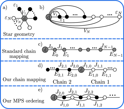
Figure 1: a,b) The star-geometry. a) The impurity orbital “d” hybridizes with a half-filled bath of conduction electrons. Here and below, gray circles denote partially filled orbitals, black/white fully-occupied/empty ones; b) The topologically equivalent chain with long-range hoppings, with orbitals ordered according to their increasing energy $\epsilon_{k}$; c) The conventional chain mapping, mixing all conduction states and leading to partly-filled orthogonal conduction orbitals; d) Chain-mapping separating filled from empty conduction electrons; e) Ordering of the sites used in our MPS. Notice that for $T=0$ we actually use two similar half-chains with spinless orbitals.

The present Letter presents an effective strategy to perform MPS-DMRG calculations based on short-ranged chain mappings that i) show low entanglement and ii) can deal with finite temperature. The crucial idea (sketched in Fig. 1(d)) is easy to understand at $T=0$: one needs to separate empty and filled conduction orbitals by constructing two separate tight-binding chains, independently coupled to the impurity orbital, an idea which has proven beneficial in Lanczos-based exact diagonalization already Lu et al. (2014). To expand on that, allowing $T>0$ calculations, we borrow some of the tools developed in the field of open quantum systems with bosonic environments, notably the thermo-field transformation Takahashi and Umezawa (1975); de Vega and Bañuls (2015), with fermionic applications to quantum transport Schwarz et al. (2018) and quench dynamics Nüßeler et al. (2020). The result is a very efficient MPS-DMRG impurity solver, with short-range couplings and low entanglement, which works also at finite $T$, and can be extended to deal with multiple orbitals Bauernfeind et al. (2017) and out-of-equilibrium phenomena.

Model and methods — The SIAM Anderson (1961) consists of a single spin-full impurity orbital hybridizing with a bath of free conduction electrons:

$$\widehat{H}_{\scriptscriptstyle\mathrm{SIAM}}(t)=\widehat{H}_{\text{loc}}(t)+\widehat{H}_{\text{hyb}}+\widehat{H}_{\text{cond}}\;.$$ (1)

The local Hamiltonian describes the impurity:

$$\widehat{H}_{\text{loc}}(t)=\sum_{\sigma}\varepsilon_{d}(t){\hat{d}^{\dagger}}_{\sigma}{\hat{d}^{\phantom{\dagger}}}_{\sigma}+U\,{\hat{n}^{\phantom{\dagger}}}_{\uparrow}{\hat{n}^{\phantom{\dagger}}}_{\downarrow}\;,$$ (2)

where ${\hat{d}^{\dagger}}_{\sigma}$ creates an electron with spin $\sigma=\uparrow,\downarrow$ in the impurity orbital, ${\hat{n}^{\phantom{\dagger}}}_{\sigma}={\hat{d}^{\dagger}}_{\sigma}{\hat{d}^{\phantom{\dagger}}}_{\sigma}$ is the number operator, and $U$ the on-site Hubbard repulsion. Here we could allow for a time-dependent impurity level $\varepsilon_{d}(t)=E_{d}(t)-\mu$, where $\mu$ denotes the chemical potential of the conduction electron bath, and even for a time-dependent $U(t)$, for possible applications to non-equilibrium problems. The impurity-bath hybridization is given by:

$$\widehat{H}_{\text{hyb}}=\sum_{\sigma}\sum_{k}V_{k}\,\Big{(}{\hat{d}^{\dagger}}_{\sigma}\,{\hat{c}^{\phantom{\dagger}}}_{k,\sigma}+{\hat{c}^{\dagger}}_{k,\sigma}\,{\hat{d}^{\phantom{\dagger}}}_{\sigma}\Big{)}\;,$$ (3)

where $V_{k}$ is a (real) hybridization matrix element and ${\hat{c}^{\dagger}}_{k,\sigma}$ creates a conduction electron in an orbital labelled by $k$, and $\widehat{H}_{\text{cond}}=\sum_{k,\sigma}\;\epsilon_{k}\,{\hat{c}^{\dagger}}_{k,\sigma}\,{\hat{c}^{\phantom{\dagger}}}_{k,\sigma}$. Here $\epsilon_{k}$ denotes energies referred to the conduction electron chemical potential $\mu$.

Following Wilson’s NRG approach idea Wilson (1975), it is tempting to recast this problem into a nearest-neighbour tight-binding form, to better apply MPS/DMRG algorithms. Indeed, the only electronic orbital that couples to the impurity is the combination ${\hat{a}^{\phantom{\dagger}}}_{0,\sigma}=J_{0}^{-1}\sum_{k}V_{k}{\hat{c}^{\phantom{\dagger}}}_{k,\sigma}$, where $J_{0}=\sqrt{\sum_{k}V_{k}^{2}}$ enforces the correct normalization. Hence the problem can be cast into a tridiagonal tight-binding form by standard techniques, such as linear discretization plus Lanczos tridiagonalization or orthogonal polynomials Chin et al. (2010); Prior et al. (2010); Gautschi (2004), as sketched in Fig. 1(c). But this is, unfortunately, not a good route: as shown in Ref. Wolf et al. (2014b), the entanglement properties of such a tight-binding chain scale worse than the plain application of MPS/DMRG techniques to the so-called star geometry, where one orders the orbitals according to their energy $\epsilon_{k}$, from the most negative ($\epsilon_{k}<0$) occupied orbitals up to the $\epsilon_{k}>0$ unoccupied ones, allowing for the appropriate long-ranged hybridization couplings $V_{k}$ (see Fig. 1(a,b)).

Our mapping — We start discussing the zero-temperature case, omitting the spin index for a while. Let us re-define the original fermions as ${\hat{c}^{\phantom{\dagger}}}_{k}\to{\hat{c}^{\phantom{\dagger}}}_{1k}$. Their filled Fermi-sea state will be denoted by $|\mathrm{FS}_{1}\rangle=\prod_{k}\Theta(-\epsilon_{k}){\hat{c}^{\dagger}}_{1k}|0\rangle$, where $\Theta(\cdot)$ is the Heaviside theta-function. Following Takahashi and Umezawa Takahashi and Umezawa (1975), we introduce a second ancillary fermionic operator ${\hat{c}^{\phantom{\dagger}}}_{2k}$, which will not couple to the impurity, and put in a fiducial ancillary state given by their filled Fermi sea $|\mathrm{FS}_{2}\rangle=\prod_{k}\Theta(-\epsilon_{k}){\hat{c}^{\dagger}}_{2k}|0\rangle$. Define now a new canonical set of fermionic operators as follows Takahashi and Umezawa (1975); de Vega and Bañuls (2015); Nüßeler et al. (2020); Schwarz et al. (2018):

$$\left(\begin{array}[]{c}{\hat{f}^{\phantom{\dagger}}}_{1k}\\ {\hat{f}^{\phantom{\dagger}}}_{2k}\end{array}\right)=\left(\begin{array}[]{rr}\cos\theta_{k}&-\sin\theta_{k}\\ \sin\theta_{k}&\cos\theta_{k}\end{array}\right)\left(\begin{array}[]{c}{\hat{c}^{\phantom{\dagger}}}_{1k}\\ {\hat{c}^{\dagger}}_{2k}\end{array}\right)\;.$$ (4)

While originally introduced to deal with finite temperature, this transformation will turn out extremely useful even at $T=0$. For $\cos\theta_{k}=\Theta(\epsilon_{k})$ and $\sin\theta_{k}=\Theta(-\epsilon_{k})$, Eq. 4 is a compact way of writing a conditional (on $\epsilon_{k}$) intertwined particle-hole transformations — ${\hat{f}^{\phantom{\dagger}}}_{1k}={\hat{c}^{\phantom{\dagger}}}_{1k}$ and ${\hat{f}^{\phantom{\dagger}}}_{2k}={\hat{c}^{\dagger}}_{2k}$ for $\epsilon_{k}>0$, while ${\hat{f}^{\phantom{\dagger}}}_{1k}=-{\hat{c}^{\dagger}}_{2k}$ and ${\hat{f}^{\phantom{\dagger}}}_{2k}={\hat{c}^{\phantom{\dagger}}}_{1k}$ for $\epsilon_{k}<0$ — so that $\forall k$:

$${\hat{f}^{\phantom{\dagger}}}_{1k}|\mathrm{FS}_{1}\rangle\otimes|\mathrm{FS}_{2}\rangle=0\hskip 14.22636pt\mbox{and}\hskip 14.22636pt{\hat{f}^{\dagger}}_{2k}|\mathrm{FS}_{1}\rangle\otimes|\mathrm{FS}_{2}\rangle=0\;,$$ (5)

hence $|\mathrm{FS}_{1}\rangle\otimes|\mathrm{FS}_{2}\rangle$ is the vacuum of the ${\hat{f}^{\phantom{\dagger}}}_{1k}$, denoted by $|\emptyset_{1}\rangle$, and the fully filled state of the ${\hat{f}^{\phantom{\dagger}}}_{2k}$, denoted by $|\mathrm{F}_{2}\rangle$. So, Eq. (4), with the $T=0$ choice $\cos\theta_{k}=\Theta(\epsilon_{k})$ and $\sin\theta_{k}=\Theta(-\epsilon_{k})$, implies $|\mathrm{FS}_{1}\rangle\otimes|\mathrm{FS}_{2}\rangle\equiv|\emptyset_{1}\rangle\otimes|\mathrm{F}_{2}\rangle$.

Now, we supplement our SIAM with an ancillary conduction term $\sum_{k}\epsilon_{k}\,{\hat{c}^{\phantom{\dagger}}}_{2k}\,{\hat{c}^{\dagger}}_{2k}$, such that the full kinetic energy reads:

$$\sum_{k}\epsilon_{k}\,\Big{(}{\hat{c}^{\dagger}}_{1k}\,{\hat{c}^{\phantom{\dagger}}}_{1k}+{\hat{c}^{\phantom{\dagger}}}_{2k}\,{\hat{c}^{\dagger}}_{2k}\Big{)}=\sum_{k}\epsilon_{k}\Big{(}{\hat{f}^{\dagger}}_{1k}\,{\hat{f}^{\phantom{\dagger}}}_{1k}+{\hat{f}^{\dagger}}_{2k}\,{\hat{f}^{\phantom{\dagger}}}_{2k}\Big{)}\;.$$

As for the hybridization, we have:

$$\sum_{k}V_{k}\,{\hat{d}^{\dagger}}\!\,{\hat{c}^{\phantom{\dagger}}}_{1k}=\sum_{k}\Big{(}V_{1k}\,{\hat{d}^{\dagger}}\!\,{\hat{f}^{\phantom{\dagger}}}_{1k}+V_{2k}\,{\hat{d}^{\dagger}}\!\,{\hat{f}^{\phantom{\dagger}}}_{2k}\Big{)}\;,$$ (6)

with $V_{1k}=V_{k}\,\cos\theta_{k}$ and $V_{2k}=V_{k}\,\sin\theta_{k}$. Hence the impurity hybridizes with $\epsilon_{k}>0$ ${\hat{f}^{\phantom{\dagger}}}_{1k}$-modes and $\epsilon_{k}<0$ ${\hat{f}^{\phantom{\dagger}}}_{2k}$-modes, corresponding to the original ${\hat{c}^{\phantom{\dagger}}}_{1k}$ modes, neatly separating empty and filled conduction states, a key to a low-entanglement chain mapping.

Interestingly, this naturally allows to capture the $T>0$ physics. Indeed, the expectation value of the original fermions ${\hat{c}^{\dagger}}_{1k}{\hat{c}^{\phantom{\dagger}}}_{1k}$ on the pure state $|\emptyset_{1}\rangle\otimes|{\mathrm{F}}_{2}\rangle=|\emptyset_{1},{\mathrm{F}}_{2}\rangle$ is:

$$\langle\emptyset_{1},{\mathrm{F}}_{2}|\,{\hat{c}^{\dagger}}_{1k}\,{\hat{c}^{\phantom{\dagger}}}_{1k}|\emptyset_{1},{\mathrm{F}}_{2}\rangle=\sin^{2}(\theta_{k})\;.$$ (7)

Hence the pure state $|\emptyset_{1},{\mathrm{F}}_{2}\rangle$ will effectively mimic the Fermi occupation factor for the conduction electrons provided we take: Nüßeler et al. (2020)

$$\sin^{2}(\theta_{k})\equiv\frac{1}{\textrm{e}^{\beta\epsilon_{k}}+1}\;.$$ (8)

Notice that now, for such a general $\theta_{k}$, $|\emptyset_{1},{\mathrm{F}}_{2}\rangle\neq|\mathrm{FS}_{1}\rangle\otimes|\mathrm{FS}_{2}\rangle$: the pure-state $|\emptyset_{1},{\mathrm{F}}_{2}\rangle$ captures thermal expectation values for the ${\hat{c}^{\phantom{\dagger}}}_{1k}$, with a highly non-trivial structure of the states for the original fermions.

We carry out separate chain mappings for empty and filled modes to preserve their product state property de Vega and Bañuls (2015); Schwarz et al. (2018), with initial orbitals ${\hat{a}^{\phantom{\dagger}}}_{i,0}=J_{i,0}^{-1}\sum_{k}V_{i,k}{\hat{f}^{\phantom{\dagger}}}_{ik}$ ($i=1,2$). After reinstalling spin indices, we end up with the final tight-binding Hamiltonian

$$\widehat{H}_{\scriptscriptstyle\mathrm{SIAM}}=\widehat{H}_{\text{loc}}+\sum_{\sigma}\sum_{i=1}^{2}\bigg{(}J_{i,0}\left({\hat{d}^{\dagger}}_{\sigma}\,{\hat{a}^{\phantom{\dagger}}}_{i,0,\sigma}+\mathrm{H.c.}\right)+\sum_{n=1}^{\infty}\left(J_{i,n}{\hat{a}^{\dagger}}_{i,n,\sigma}{\hat{a}^{\phantom{\dagger}}}_{i,n-1,\sigma}+\mathrm{H.c.}\right)+\sum_{n=0}^{\infty}E_{i,n}\,{\hat{a}^{\dagger}}_{i,n,\sigma}{\hat{a}^{\phantom{\dagger}}}_{i,n,\sigma}\bigg{)}\;.$$ (9)

While the Hamiltonian in Eq. (9) has perfect chain geometry, see Fig. 1(d), we employed a slightly different ordering of the sites, sketched in Fig. 1(e). Similar ideas were recently used to study quantum transport Chen et al. (2020) and 1D systems with periodic boundary conditions Haller et al. (2020); Contessi et al. (2020). This ordering significantly reduces the entanglement at $T>0$, but requires next-nearest neighbor couplings, which we deal with by using the time-dependent variational principle (TDVP) Lubich et al. (2015); Haegeman et al. (2011, 2016); Paeckel et al. (2019); Bauernfeind and Aichhorn (2020); Kohn et al. (2020). We chose 2-site TDVP and checked projection errors by comparison with different MPS orderings (see SM). A more detailed analysis of these issues will be presented elsewhere.

In the following we are interested in the retarded Green’s function

$$G^{\scriptscriptstyle\mathrm{R}}_{\sigma}(t) =-i\Theta(t)\,{\mathrm{Tr}}_{\scriptscriptstyle\mathrm{S}}\left(\{{\hat{d}^{\phantom{\dagger}}}_{\sigma}(t),{\hat{d}^{\dagger}}_{\sigma}(0)\}\hat{\rho}_{\scriptscriptstyle\mathrm{S}}\right)\;,$$ (10)

where ${\hat{d}^{\phantom{\dagger}}}_{\sigma}(t)$ is the Heisenberg impurity operator, $\hat{\rho}_{\scriptscriptstyle\mathrm{S}}$ the thermal density matrix of the system, and $\{\cdot,\cdot\}$ denotes the anti-commutator. The Fourier transform of the $G^{\scriptscriptstyle\mathrm{R}}_{\sigma}(t)$ provides the experimentally accessible spectral function $A_{\sigma}(\omega)=-\frac{1}{\pi}\text{Im}\,\int_{-\infty}^{\infty}\mathrm{d}t\ \textrm{e}^{i\omega t}\,G^{\scriptscriptstyle\mathrm{R}}_{\sigma}(t)$.

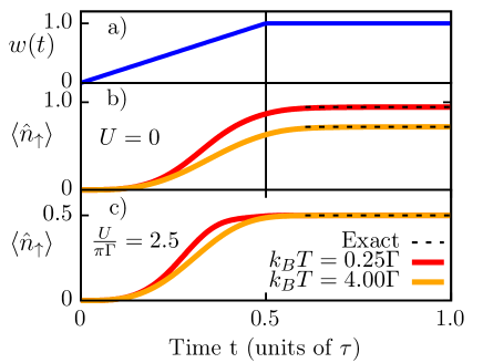
Figure 2: Top: Equilibration scheme employed to construct the thermal state of the system, see text for explanation. Local and hybridization terms are ramped-up linearly and kept constant for $t/\tau>0.5$. Below: Evolution of $\langle\hat{n}_{\uparrow}\rangle$ for the noninteracting $U=0$ (b) and particle-hole symmetric case $U=2.5\pi\Gamma$ (c) at fixed impurity level energy $\varepsilon_{d}=-1.25\pi\Gamma$. Here $\tau=8\hbar/\Gamma$ and bond dimension $D=150$.

In general, $\hat{\rho}_{\scriptscriptstyle\mathrm{S}}$ is the state where impurity and bath are in thermal equilibrium. Physically, equilibrium can be established by starting from a state where impurity and bath are isolated, by slowly turning on the hybridization between the two. At $T=0$, however, there is a short-cut, and $\hat{\rho}_{\scriptscriptstyle\mathrm{S}}$ can be obtained by a DMRG ground state (GS) search Ganahl et al. (2015); Wolf et al. (2014b); Bauernfeind et al. (2017). For finite $T>0$ we cannot do that, and, following the previous idea of a real-time equilibration, the thermal state $\hat{\rho}_{\scriptscriptstyle\mathrm{S}}$ is obtained through a TDVP evolution, working particularly well at higher temperatures, as detailed in the SM: 1) we initialize a state with empty impurity $|0\rangle$ and “thermal” conduction electrons, with a MPS pure state $|\psi_{0}\rangle=|0\rangle\otimes|\emptyset_{1},{\mathrm{F}}_{2}\rangle$; 2) We evolve the system by slowly ramping-up the local and hybridization terms as $\widehat{H}_{\scriptscriptstyle\mathrm{SIAM}}^{\text{eq}}(t)=w(t)(\widehat{H}_{\text{loc}}+\widehat{H}_{\text{hyb}})+\widehat{H}_{\text{cond}}$, with $w(t)$ starting from zero and linearly approaching one, see Fig. 2(a), until reaching $\widehat{H}_{\scriptscriptstyle\mathrm{SIAM}}$; 3) We finally relax the system with $\widehat{H}_{\scriptscriptstyle\mathrm{SIAM}}$, getting to a final MPS pure state $|\mathrm{E}\rangle$ effectively encoding the correct equilibrium state, such that $\hat{\rho}_{\scriptscriptstyle\mathrm{S}}={\rm Tr}_{\scriptscriptstyle\mathrm{anc}}\left(|\mathrm{E}\rangle\langle\mathrm{E}|\right)$.

To calculate $G^{\scriptscriptstyle\mathrm{R}}_{\sigma}$ in Eq. 10 we first split it as $G^{\scriptscriptstyle\mathrm{R}}_{\sigma}(t)=\Theta(t)\left(G^{>}_{\sigma}(t)-G^{<}_{\sigma}(t)\right)$, where $G^{>}_{\sigma}$ and $G^{<}_{\sigma}$ are the greater and lesser Green’s functions, respectively, calculated in separate simulations. For the discussion we focus on $iG^{>}_{\sigma}(t)={\rm Tr}_{\scriptscriptstyle\mathrm{S}}({\hat{d}^{\phantom{\dagger}}}_{\sigma}(t){\hat{d}^{\dagger}}_{\sigma}\hat{\rho}_{\scriptscriptstyle\mathrm{S}})$, as $G^{<}_{\sigma}$ is similar. After writing explicitly the time dependence of the Heisenberg operators and reordering operators within the trace we get:

$$iG^{>}_{\sigma}(t)={\rm Tr}_{\scriptscriptstyle\mathrm{S}+\scriptscriptstyle\mathrm{anc}}\left(\textrm{e}^{-i\hat{H}t/\hbar}{\hat{d}^{\dagger}}_{\sigma}\,|\mathrm{E}\rangle\langle\mathrm{E}|\,\textrm{e}^{i\hat{H}t/\hbar}{\hat{d}^{\phantom{\dagger}}}_{\sigma}\right)\;.$$ (11)

Note that we traced over both the physical fermions and over the ancillary ones, as required by $\hat{\rho}_{\scriptscriptstyle\mathrm{S}}$. Defining states $|\phi^{>}_{L}(t)\rangle=\textrm{e}^{-i\hat{H}t/\hbar}\,{\hat{d}^{\dagger}}_{\sigma}\,|\mathrm{E}\rangle$ and $\langle\phi^{>}_{R}(t)|=\langle\mathrm{E}|\,\textrm{e}^{i\hat{H}t/\hbar}{\hat{d}^{\phantom{\dagger}}}_{\sigma}$, calculated by two independent TDVP evolutions, we finally rewrite $iG^{>}_{\sigma}(t)={\rm Tr}(|\phi^{>}_{L}(t)\rangle\langle\phi^{>}_{R}(t)|)=\langle\phi^{>}_{R}(t)|\phi^{>}_{L}(t)\rangle$.

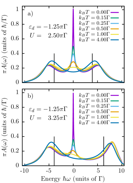
Figure 3: Spectral function as obtained from the Fourier transform of the retarded Green’s function at different temperatures, showing the disappearance of the Kondo peak for increasing $T$. The interaction is $U=2.5\pi\Gamma$ for the symmetric (a) and $U=3.25\pi\Gamma$ for the non-symmetric case (b). Vertical lines mark impurity level energies at $\varepsilon_{d}$ and $\varepsilon_{d}+U$. In the symmetric case we can estimate a Kondo temperature $k_{B}T_{K}\sim 0.07\Gamma$.

Results — In our simulations we used a semi-elliptical fermion bath hybridization with half bandwidth $W$ and coupling $\Gamma$, which in the continuum limit gives $\sum_{k}V_{k}^{2}\delta(\epsilon-\epsilon_{k})=\Gamma\sqrt{1-(\epsilon/W)^{2}}/\pi$. We fixed $W=10\Gamma$ and the impurity energy level $\varepsilon_{d}=-1.25\pi\Gamma$. From here on we use $\Gamma$ as our unit of energy. As discussed, our method involves two steps: First, we determine the equilibrium pure state $|\mathrm{E}\rangle$ either by a direct DMRG GS-search ($T=0$) or by a dynamical ramp-up, see Fig. 2(a), of $\widehat{H}_{\text{loc}}$ and $\widehat{H}_{\text{hyb}}$ ($T>0$). Second, we calculate the Green’s function by TDVP evolutions starting from $|\rm E\rangle$.

To test the first (equilibration) step we start from the empty impurity state $|\psi_{0}\rangle=|0\rangle\otimes|\emptyset_{1},{\mathrm{F}}_{2}\rangle$ and study the evolution of the spin-up impurity occupation $\langle{\hat{n}^{\phantom{\dagger}}}_{\uparrow}\rangle$ and benchmark it against exact values, for the noninteracting case ($U=0$), Fig. 2(b), where exact diagonalization is possible, and for the particle-hole symmetric case ($\varepsilon_{d}=-1.25\pi\Gamma$, $U=2.5\pi\Gamma$), Fig. 2(c), where the impurity is half-filled at any temperature $\langle\hat{n}_{\uparrow}\rangle=\langle\hat{n}_{\downarrow}\rangle=1/2$. We find that $\langle{\hat{n}^{\phantom{\dagger}}}_{\uparrow}\rangle$, starting from $0$, converges to the exact values at the end of the equilibration in all cases.

In the second step we calculate the Green’s function and — by means of a Fourier transform — the corresponding $A(\omega)$. To obtain a smooth $A(\omega)$ we employ “linear prediction” White and Affleck (2008); Barthel et al. (2009); Ganahl et al. (2015) to extrapolate simulation data to longer times. In the symmetric case, at sufficiently strong repulsion $U$, we find two symmetrically located broad peaks due to the impurity close to energies $\epsilon_{d}$ and $\epsilon_{d}+U$, and a Kondo peak at the Fermi energy, see Fig. 3(a) Horvatić et al. (1987). We observe the disappearance of the Kondo peak as $T$ increases. For the non-symmetric case of Fig. 3(b), at larger $U$, the Kondo peak becomes narrower but is still located at the Fermi energy.

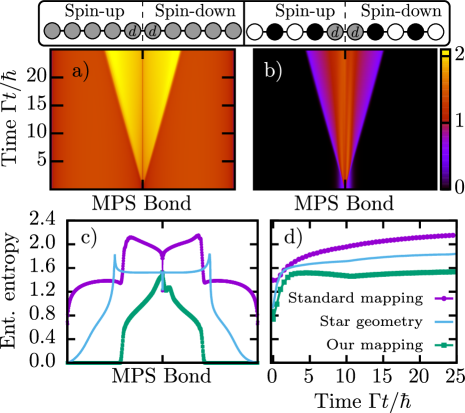
Figure 4: Top: Evolution of the entanglement entropy along the MPS for the original chain method (a) and our work (b) in the symmetric SIAM at T=0. Bottom: (c) The entanglement entropy at time $t=25\hbar/\Gamma$ and (d) time-evolution of the maximum entropy for the original chain mapping, Fig. 1(c), our chain mapping, Fig. 1(e), and the star geometry, Fig. 1(b).

We now show how efficient is our mapping in terms of entanglement. We consider here $T=0$, where we use a modified MPS structure: in addition to the orderings in Fig. 1(e), spin degrees of freedom are spatially separated — which is known to be very efficient Saberi et al. (2008); Ganahl et al. (2015); Rams and Zwolak (2020) — with spin-up on the left half of the MPS, spin-down on the right half, and the impurity in the middle. Fig. 4(a,b) show that our mapping leads to significantly lower entanglement entropy with respect to a standard chain mapping, with a characteristic “light-cone” spreading of entanglement, typical of short-ranged models. Fig. 4(c) shows a snapshot of the entanglement entropy across the whole MPS at time $t=25\hbar/\Gamma$: interestingly, not only we drastically improve on the standard chain mapping, but we also significantly improve on the star geometry (see SM for details). Fig. 4(d) shows the time-evolution of the maximum entanglement in the MPS: the original chain mapping, and also the star geometry, seem to show a logarithmic growth of entanglement, consistently with the analysis of Ref. He and Millis (2017), while the maximum entanglement entropy of our mapping seems to saturate, or in any case increase much more slowly. Finally, let us mention that our method shows excellent scaling with the bath size, as increasing the number of sites will only lead to an extension of the zero entanglement region (see Fig. 4(b)) at the end of the chain, barely increasing the computational costs (see SM for details).

Conclusions — We presented an efficient chain-mapping-based method to simulate Anderson impurity models using Matrix Product States. Our method overcomes a major problem of the original chain mapping, where mixing empty and filled sites led to large entanglement within the chain. Separating empty from filled sites and mapping them into separate chains, we drastically reduced the entanglement, providing significant performance improvements. In contrast to the star geometry, our method does not involve long-range couplings, but only next nearest neighbor terms. Using a thermo-field transformation the idea neatly generalizes to finite temperatures, where we demonstrated its capabilities by studying the Kondo physics regime. Future research directions include the application to non-equilibrium dynamics, and the implementation of the DMFT loop, where multi-orbital problems are within reach Ganahl et al. (2015); Bauernfeind et al. (2017).

We thank A. Amaricci, M. Capone, M. Dalmonte, M. Seclì and E. Tosatti for discussions, and U. Schollwöck for a careful reading of the manuscript. Research was partly supported by EU Horizon 2020 under ERC-ULTRADISS, Grant Agreement No. 834402. GES acknowledges that his research has been conducted within the framework of the Trieste Institute for Theoretical Quantum Technologies (TQT). Simulations were performed using the ITensor library Fishman et al. (2020).

References

- Anderson (1961) P. W. Anderson, Phys. Rev. 124, 41 (1961).
- Kondo (1964) J. Kondo, Progress of theoretical physics 32, 37 (1964).
- Hewson (1997) A. C. Hewson, The Kondo problem to heavy fermions (Cambridge University Press, 1997).
- Metzner and Vollhardt (1989) W. Metzner and D. Vollhardt, Phys. Rev. Lett. 62, 324 (1989).
- Georges et al. (1996) A. Georges, G. Kotliar, W. Krauth, and M. J. Rozenberg, Rev. Mod. Phys. 68, 13 (1996).
- Gull et al. (2011) E. Gull, A. J. Millis, A. I. Lichtenstein, A. N. Rubtsov, M. Troyer, and P. Werner, Rev. Mod. Phys. 83, 349 (2011).
- Rubtsov et al. (2005) A. N. Rubtsov, V. V. Savkin, and A. I. Lichtenstein, Phys. Rev. B 72, 035122 (2005).
- Werner et al. (2006) P. Werner, A. Comanac, L. de’ Medici, M. Troyer, and A. J. Millis, Phys. Rev. Lett. 97, 076405 (2006).
- Bulla et al. (2008) R. Bulla, T. A. Costi, and T. Pruschke, Rev. Mod. Phys. 80, 395 (2008).
- Stadler et al. (2015) K. M. Stadler, Z. P. Yin, J. von Delft, G. Kotliar, and A. Weichselbaum, Phys. Rev. Lett. 115, 136401 (2015).
- Bulla (1999) R. Bulla, Phys. Rev. Lett. 83, 136 (1999).
- Žitko and Pruschke (2009) R. Žitko and T. Pruschke, Phys. Rev. B 79, 085106 (2009).
- Deng et al. (2013) X. Deng, J. Mravlje, R. Žitko, M. Ferrero, G. Kotliar, and A. Georges, Phys. Rev. Lett. 110, 086401 (2013).
- Mitchell et al. (2014) A. K. Mitchell, M. R. Galpin, S. Wilson-Fletcher, D. E. Logan, and R. Bulla, Phys. Rev. B 89, 121105 (2014).
- White (1992) S. R. White, Phys. Rev. Lett. 69, 2863 (1992).
- Schollwöck (2005) U. Schollwöck, Rev. Mod. Phys. 77, 259 (2005).
- Schollwöck (2011) U. Schollwöck, Annals of Physics 326, 96 (2011).
- Montangero (2018) S. Montangero, Introduction to Tensor Network Methods (Springer International Publishing, 2018).
- Wolf et al. (2015) F. A. Wolf, A. Go, I. P. McCulloch, A. J. Millis, and U. Schollwöck, Phys. Rev. X 5, 041032 (2015).
- Linden et al. (2020) N.-O. Linden, M. Zingl, C. Hubig, O. Parcollet, and U. Schollwöck, Phys. Rev. B 101, 041101 (2020).
- García et al. (2004) D. J. García, K. Hallberg, and M. J. Rozenberg, Phys. Rev. Lett. 93, 246403 (2004).
- Wolf et al. (2014a) F. A. Wolf, I. P. McCulloch, O. Parcollet, and U. Schollwöck, Phys. Rev. B 90, 115124 (2014a).
- Ganahl et al. (2015) M. Ganahl, M. Aichhorn, H. G. Evertz, P. Thunström, K. Held, and F. Verstraete, Phys. Rev. B 92, 155132 (2015).
- Wolf et al. (2014b) F. A. Wolf, I. P. McCulloch, and U. Schollwöck, Phys. Rev. B 90, 235131 (2014b).
- Bauernfeind et al. (2017) D. Bauernfeind, M. Zingl, R. Triebl, M. Aichhorn, and H. G. Evertz, Phys. Rev. X 7, 031013 (2017).
- Wilson (1975) K. G. Wilson, Rev. Mod. Phys. 47, 773 (1975).
- Lu et al. (2014) Y. Lu, M. Höppner, O. Gunnarsson, and M. W. Haverkort, Phys. Rev. B 90, 085102 (2014).
- He and Millis (2017) Z. He and A. J. Millis, Phys. Rev. B 96, 085107 (2017).
- Takahashi and Umezawa (1975) Y. Takahashi and H. Umezawa, Collective Phenomena 2, 55 (1975).
- de Vega and Bañuls (2015) I. de Vega and M.-C. Bañuls, Phys. Rev. A 92, 052116 (2015).
- Schwarz et al. (2018) F. Schwarz, I. Weymann, J. von Delft, and A. Weichselbaum, Phys. Rev. Lett. 121, 137702 (2018).
- Nüßeler et al. (2020) A. Nüßeler, I. Dhand, S. F. Huelga, and M. B. Plenio, Phys. Rev. B 101, 155134 (2020).
- Chin et al. (2010) A. W. Chin, Á. Rivas, S. F. Huelga, and M. B. Plenio, Journal of Mathematical Physics 51, 092109 (2010).
- Prior et al. (2010) J. Prior, A. W. Chin, S. F. Huelga, and M. B. Plenio, Physical review letters 105, 050404 (2010).
- Gautschi (2004) W. Gautschi, Orthogonal polynomials (Oxford University Press, New York, 2004).
- Chen et al. (2020) T. Chen, V. Balachandran, C. Guo, and D. Poletti, Phys. Rev. E 102, 012155 (2020).
- Haller et al. (2020) A. Haller, M. Rizzi, and M. Filippone, Phys. Rev. Research 2, 023058 (2020).
- Contessi et al. (2020) D. Contessi, D. Romito, M. Rizzi, and A. Recati (2020), eprint arXiv:2009.09504.
- Lubich et al. (2015) C. Lubich, I. V. Oseledets, and B. Vandereycken, SIAM Journal on Numerical Analysis 53, 917 (2015).
- Haegeman et al. (2011) J. Haegeman, J. I. Cirac, T. J. Osborne, I. Pižorn, H. Verschelde, and F. Verstraete, Phys. Rev. Lett. 107, 070601 (2011).
- Haegeman et al. (2016) J. Haegeman, C. Lubich, I. Oseledets, B. Vandereycken, and F. Verstraete, Phys. Rev. B 94, 165116 (2016).
- Paeckel et al. (2019) S. Paeckel, T. Köhler, A. Swoboda, S. R. Manmana, U. Schollwöck, and C. Hubig, Annals of Physics 411, 167998 (2019).
- Bauernfeind and Aichhorn (2020) D. Bauernfeind and M. Aichhorn, SciPost Phys. 8, 24 (2020).
- Kohn et al. (2020) L. Kohn, P. Silvi, M. Gerster, M. Keck, R. Fazio, G. E. Santoro, and S. Montangero, Phys. Rev. A 101, 023617 (2020).
- White and Affleck (2008) S. R. White and I. Affleck, Phys. Rev. B 77, 134437 (2008).
- Barthel et al. (2009) T. Barthel, U. Schollwöck, and S. R. White, Phys. Rev. B 79, 245101 (2009).
- Horvatić et al. (1987) B. Horvatić, D. Sokcević, and V. Zlatić, Phys. Rev. B 36, 675 (1987).
- Saberi et al. (2008) H. Saberi, A. Weichselbaum, and J. von Delft, Phys. Rev. B 78, 035124 (2008).
- Rams and Zwolak (2020) M. M. Rams and M. Zwolak, Phys. Rev. Lett. 124, 137701 (2020).
- Fishman et al. (2020) M. Fishman, S. R. White, and E. M. Stoudenmire (2020), eprint arXiv:2007.14822.
- Serafini (2017) A. Serafini, Quantum continuous variables: a primer of theoretical methods (CRC Press, 2017).
- Schröder and Chin (2016) F. A. Y. N. Schröder and A. W. Chin, Phys. Rev. B 93, 075105 (2016).
- Singh et al. (2010) S. Singh, R. N. C. Pfeifer, and G. Vidal, Phys. Rev. A 82, 050301 (2010).
- Singh et al. (2011) S. Singh, R. N. C. Pfeifer, and G. Vidal, Phys. Rev. B 83, 115125 (2011).
- Silvi et al. (2019) P. Silvi, F. Tschirsich, M. Gerster, J. Jünemann, D. Jaschke, M. Rizzi, and S. Montangero, SciPost Phys. Lect. Notes 8 (2019).